A Raman lidar tropospheric water vapour climatology and height-resolved trend analysis over Payerne, Switzerland

Water vapour is the strongest greenhouse gas in our atmosphere, and its strength and its dependence on temperature lead to a strong feedback mechanism in both the troposphere and the stratosphere. Raman water vapour lidars can be used to make high-vertical-resolution measurements on the order of tens of metres, making height-resolved trend analyses possible. Raman water vapour lidars have not typically been used for trend analyses, primarily due to the lack of long-enough time series. However, the Raman Lidar for Meteorological Observations (RALMO), located in Payerne, Switzerland, is capable of making operational water vapour measurements and has one of the longest ground-based and well-characterized data sets available. We have calculated an 11.5-year water vapour climatology using RALMO measurements in the troposphere. Our study uses nighttime measurements during mostly clear conditions, which creates a natural selection bias. The climatology shows that the highest water vapour specific-humidity concentrations are in the summer months and the lowest in the winter months. We have also calculated the geophysical variability of water vapour. The percentage of variability of water vapour in the free troposphere is larger than in the boundary layer.

We have also determined water vapour trends from 2009 to 2019. We first calculate precipitable water vapour (PWV) trends for comparison with the majority of water vapour trend studies. We detect a nighttime precipitable water vapour trend of 1.3 mm per decade using RALMO measurements, which is significant at the 90 % level. The trend is consistent with a 1.38 ^∘C per decade surface temperature trend detected by coincident radiosonde measurements under the assumption that relative humidity remains constant; however, it is larger than previous water vapour trend values. We compare the nighttime RALMO PWV trend to daytime and nighttime PWV trends using operational radiosonde measurements and find them to agree with each other. We cannot detect a bias between the daytime and nighttime trends due to the large uncertainties in the trends. For the first time, we show height-resolved increases in water vapour through the troposphere. We detect positive tropospheric water vapour trends ranging from a 5 % change in specific humidity per decade to 15 % specific humidity per decade depending on the altitude. The water vapour trends at five layers are statistically significant at or above the 90 % level.

1 Introduction

Water vapour is the atmosphere's most important minor constituent. It plays a significant role in almost all aspects of the atmosphere, including dynamics, circulation, radiative processes, and chemistry with other molecular and particulate species. Water vapour accounts for 60 % of the greenhouse effect for clear skies (Kiehl and Trenberth, 1997) and has a significant feedback response to increases in temperature. It is, in this sense, Earth's “strongest” natural greenhouse gas. In fact, the temperature increase due to a doubling in CO₂ would be magnified to twice its predicted change from CO₂ alone if water vapour feedback were included in global climate (Held and Soden, 2000). While the majority of water vapour feedback is due to infrared absorption in the upper troposphere and lower stratosphere (UTLS), the change in lower and mid-tropospheric water vapour also has large implications for the hydrologic cycle and water vapour feedback (Dessler et al., 2013; Held and Soden, 2006). Tropospheric water vapour plays a key and complicated role in the hydrologic cycle, and it remains unclear how increases in water vapour affect precipitation rates, the chance of extreme precipitation events or droughts. High-vertical-resolution water vapour profiles on the order of 100 m are extremely useful for modellers to accurately reproduce convection (Weckwerth et al., 1999). Tropospheric water vapour climatologies and trends are also critical to understanding and modelling water vapour's impact on global circulation systems. Tropospheric water vapour is predicted to increase by 7 % for every 1 ^∘C increase in temperature in the lower troposphere and at even higher percentages (up to 15 %) in the UTLS under the assumption that relative humidity is conserved (Held and Soden, 2000; Sherwood et al., 2010).

Measuring an atmospheric water vapour trend is difficult due to the fact that the magnitude of the water vapour concentration at a given altitude in the troposphere can change by more than 100 % on a daily basis. Due to this huge variation, quantifying water vapour trends requires a level of precision and consistency in the measurements which is practically difficult to achieve. Early studies of water vapour trends in the troposphere were typically conducted with radiosondes (Hense et al., 1988; Ross and Elliot, 1996, 2001). However, the trends calculated in those studies were most often not significant, and their magnitudes varied greatly. Radiosonde biases have now been well documented, and data sets require significant corrections and homogenization in order to be used (Elliott and Gaffen, 1991; McCarthy et al., 2009; Miloshevich et al., 2009). The GCOS Reference Upper Air Network (GRUAN) has recently made a significant step in homogenizing and correcting many modern radiosondes so that they can be more reliably integrated into trend analyses (Miloshevich et al., 2009; Immler et al., 2010; Dirksen et al., 2014).

Since radiosonde measurements can require significant corrections, water vapour trend and climatology studies moved towards including other instruments such as microwave radiometers (Morland et al., 2009; Hocke et al., 2011), satellite-based instruments like the microwave limb sounders (Hegglin et al., 2014; Khosrawi et al., 2018), global positioning systems (GPS, Jin et al., 2007; Wang et al., 2016), and reanalyses models (Trenberth et al., 2005). However, the majority of these instruments can only measure columns of water vapour or partial column profiles. Most satellite-based instruments are capable of measuring water vapour down to 300 hPa, or roughly 9 km altitude (Hegglin et al., 2013), but a few, like the Atmospheric Infrared Sounder (AIRS) instrument on the Aqua satellite, can accurately measure through the troposphere (Trent et al., 2019). However, while satellite measurements provide excellent global coverage, their vertical resolutions are typically on the order of kilometres, which limits their ability to capture water vapour's large variability with altitude. Unlike these instruments, a Raman water vapour lidar has the ability to measure high-resolution water vapour profiles in the troposphere (on the order of metres) as well as calculate column measurements (Melfi, 1972; Whiteman, 2003). Lidar's high vertical resolution compared to microwave limb sounders or microwave radiometers makes them ideal instruments for studying the evolution of water vapour in the troposphere. The major drawbacks to using Raman lidars for trend measurements are that they are difficult to fully automate, and they cannot measure during precipitation events or in thick, cloudy conditions. As such, there have not been many lidars which have long-enough data sets with enough stability to detect statistically significant trends for climatological studies. As far as we are aware, there have been only four publications on operational Raman water vapour lidars in the last 2 decades (Goldsmith et al., 1994; Dinoev et al., 2013; Hadad et al., 2018; Reichardt et al., 2012). While these lidars have been run operationally over the last 2 decades, Raman Lidar for Meteorological Observations (RALMO) is the only one which has presented a water vapour trend study, which we show here.

Many studies have been made of precipitable water vapour (PWV) trends across Europe and Switzerland. Ross and Elliot (2001) calculated PWV trends from 1958 to 1995 using radiosonde measurements from the surface to 500 hPa and found highly geographically variable trends around the globe. Their trends calculated across Europe were insignificant and differed in sign depending on the location. Trenberth et al. (2005) also calculated global PWV trends using radiosondes and models over the ocean and found mean ocean trends of 1.6 mm per decade using measurements from 1989 to 2004. Morland et al. (2009) calculated PWV trends using a radiometer, radiosondes, and model measurements in Bern, Switzerland, from 1996 to 2007. Only the radiosondes measured a statistically significant trend at night of 0.49 mm per decade. Hocke et al. (2011) published an updated trend using homogenized measurements from two radiometers from 1994 to 2009. They did not detect an overall trend but found seasonal trends of 10 % change in PWV per decade in the summer and −15 % per decade in the winter. Other studies around Europe using measurements from the 1980s up through 2008 report positive trends on the order of 0.3–0.5 mm per decade (Nilsson and Elgered, 2008; Ning and Elgered, 2018). Hadad et al. (2018; hereafter H2018) also measured PWV trends using ground-based GPS measurements and found a positive but insignificant trend of 0.42±0.45 mm per decade. Recently, a water vapour lidar climatology using Raman lidar measurements was published by H2018 for measurements over France (45.75^∘ N, 3.125^∘ E) from 2010 to 2016. The measurements in our study have 5 more years of measurements compared to H2018. H2018 also conducted a water vapour trend analysis for their site using satellite, GPS, and ground-station measurements as well as ERA-Interim reanalyses; however, they did not include lidar measurements in their trend analysis.

While there are many PWV trend analyses, there appears to be a large gap in the community in the area of height-resolved trends. The lack of height-resolved trends may be because there are very few instruments routinely operated with the capability to measure atmospheric profiles at resolutions under 1 km in the troposphere (Wulfmeyer et al., 2015). Some studies have measured trends at the surface as well as 850 hPa using radiosondes and models (Hadad et al., 2018; Serreze et al., 2012). H2018 also uses measurements from the AIRS satellite to detect trends and calculates a water vapour mixing ratio trend of 0.13 g kg⁻¹ per decade at 950 and at 850 hPa. To our best knowledge, ours is the first study to use a Raman lidar to calculate water vapour trends at different layers in the troposphere above 850 hPa.

This study presents a tropospheric water vapour climatology and trend analysis using 11.5 years of nighttime measurements from RALMO over Payerne, Switzerland. While not the first study to produce a tropospheric water vapour climatology from a Raman lidar, it is the first to use Raman lidar measurements to calculate precipitable water vapour (PWV) trends as well as trends at different layers in the troposphere. Section 2 discusses the measurements used in this study. Section 3 describes the methodology used to create the climatology and the calculation of geophysical variability over the 10 years. Section 4 presents the trend results for both PWV and specific humidity at 10 different pressure levels up to 250 hPa. Sections 5 and 6 present the discussion and the summary and conclusions of our study, respectively.

2 Description of instruments and measurements

2.1 Raman lidar

The lidar measurements were taken by RALMO in Payerne, Switzerland (46.81^∘ N, 6.94^∘ E, 491 m a.s.l.). RALMO is a fully automated operational water vapour lidar capable of reaching into the upper troposphere at nighttime and has been designed to run autonomously with minimal downtime, high accuracy, and temporal measurement stability (Dinoev et al., 2013; Brocard et al., 2013b). Over the last 12 years, RALMO has been operating both day and night with an average of 50 % uptime, with 40 % of the downtime due to precipitation or the presence of clouds below 900 m. The other 10 % of the downtime is due to routine maintenance and equipment malfunctions. RALMO uses a tripled ND:YaG laser operating at 30 Hz with a pulse power of 300 mJ. The laser has the ability to operate at 450 mJ; however, 300 mJ was chosen to maximize the lifetime of the flashlamps. RALMO includes 12 detection channels: 4 elastic or Rayleigh scatter channels (near- and far-field), 4 pure rotational Raman channels, 2 Raman nitrogen (386.7 nm, digital and analogue) channels, and 2 water vapour (407.45 nm, digital and analogue) channels. Raw measurements are recorded as 1800-shot profiles (approximately 1 min) with an altitude resolution of 3.75 m for each channel from the surface up to 60 km. The raw 1 min profiles are called “scans”. This work uses measurements from the pure rotational Raman channels and elastic channels to calculate nightly aerosol backscatter ratios as well as measurements from the water vapour and nitrogen vibrational–rotational Raman channels to retrieve the water vapour mixing ratio profiles used in the climatology. The aerosol backscatter ratios are used to calculate transmissions and aerosol extinction for the water vapour retrieval.

The specific-humidity profiles used for the climatology and trend analysis are determined from the RALMO measurements using the optimal estimation method (OEM) retrieval introduced in Sica and Haefele (2016) for water vapour lidars. While the OEM retrieval is in units of water vapour mixing ratio, it is finally converted to specific humidity for the purposes of this trend analysis to maintain consistency with the water vapour trend literature. The OEM uses Bayes' theorem to constrain the solution space for the retrieval. It does this by adding in the use of an a priori state (x_a). A probability of any given state of the system is assigned, assuming the errors of the system are Gaussian. The optimal solution for the system is then found by minimizing the cost of the solution, where the cost is defined as

$$\begin{array}{}\text{(1)}& \begin{array}{rl}\mathrm{cost}& =\left[{\displaystyle \frac{\mathrm{1}}{\mathrm{2}}}{\left(\mathit{y}-F(\mathit{x},\mathit{b})\right)}^T{{\mathbf{S}}_{\mathit{ϵ}}}^{-\mathrm{1}}\left(\mathit{y}-F(\mathit{x},\mathit{b})\right)\right]\\ & +{\displaystyle \frac{\mathrm{1}}{\mathrm{2}}}{\left(\mathit{x}-{\mathit{x}}_{\mathrm{a}}\right)}^T{{\mathbf{S}}_{\mathrm{a}}}^{-\mathrm{1}}\left(\mathit{x}-{\mathit{x}}_{\mathrm{a}}\right).\end{array}\end{array}$$

The measurement vector is represented by y, F is the forward model for the lidar, x is the vector containing all retrieval parameters, b is the forward function parameter vector, S_a is the covariance matrix of the a priori values, and S_ϵ is the measurement covariance matrix. The cost function consists of two terms. The first term is the weighted least squares regression. The second is a regularization term, which provides additional information to the solution of an a priori state. The a priori covariance matrix and the measurement covariance matrix define the solution space of the retrieval. Minimizing the cost function produces the retrieval solution ($\widehat{\mathit{x}}$), where the solution is then the maximum a posteriori solution based on the probability distribution functions and is given by

$$\begin{array}{}\text{(2)}& \begin{array}{rl}\widehat{\mathit{x}}& ={\mathit{x}}_{\mathrm{a}}+{\left({\mathbf{K}}^T{{\mathbf{S}}_{\mathit{ϵ}}}^{-\mathrm{1}}\mathbf{K}+{{\mathbf{S}}_{\mathrm{a}}}^{-\mathrm{1}}\right)}^{-\mathrm{1}}{\mathbf{K}}^T{{\mathbf{S}}_{\mathit{ϵ}}}^{-\mathrm{1}}\left(\mathit{y}-F\left({\mathit{x}}_{\mathrm{a}}\right)\right)\\ & ={\mathit{x}}_{\mathrm{a}}+\mathbf{G}\left(\mathit{y}-F\left({\mathit{x}}_{\mathrm{a}}\right)\right),\end{array}\end{array}$$

where K refers to the Jacobian matrix, and G is the gain matrix. The Jacobian matrix is defined as $\frac{\mathrm{d}\mathit{y}}{\mathrm{d}\mathit{x}}$, and the gain matrix is $\frac{\mathrm{d}\mathit{x}}{\mathrm{d}\mathit{y}}$. An in-depth description of OEM theory applied to atmospheric physics can be found in Rodgers (2000). Sica and Haefele (2016) discussed the initial application of the OEM to Raman lidar water vapour retrievals. Details regarding the changes to the original water vapour retrieval code can be found in Appendix 4B of Hicks-Jalali (2019). Other lidar OEM retrievals and their applications are discussed in Sica and Haefele (2015) and Jalali et al. (2018) for Rayleigh temperature profile retrievals, Mahagammulla Gamage et al. (2019) for Raman temperature profile retrievals, Farhani et al. (2019) for differential absorption lidar (DIAL) ozone profile retrievals, and Mahagamulla Gamage et al. (2020) for Raman relative-humidity profile retrievals.

Processing the entire RALMO time series requires an ongoing calibration of the lidar. We have combined GRUAN radiosondes and implemented a solar background calibration method to allow a consistent calibration across the 11.5 year time series. The continuous calibration is an internal calibration technique using the solar background between the nitrogen and water vapour channels and was first introduced in Sherlock et al. (1999). The internal solar calibration method produces a relative calibration function, which is scaled to the external calibration using the GRUAN-corrected radiosondes. The calibration function has an uncertainty of 5 % of the calibration value and a corresponding uncertainty of 5 % in the final water vapour mixing ratio. The uncertainty in the solar calibration method is the same as what would be introduced by using GRUAN-corrected radiosondes for external calibration (Hicks-Jalali et al., 2019). However, by using an internal calibration function, the lidar trends remain mostly independent of an external instrument. The details of this calibration are given in Appendix A. This new calibration is consistent with the GRUAN calibration of RALMO conducted in Hicks-Jalali et al. (2019).

One of the advantages of using an OEM retrieval over the traditional method (Whiteman et al., 1992; Whiteman, 2003) is the addition of the uncertainty budget and averaging kernels for each profile. The addition of the averaging kernels in particular is important because they may be used to more accurately compare results with other instruments which utilize OEM retrievals, such as satellite-based limb-sounding instruments, Fourier-transform infrared spectrometers, or microwave radiometers. Another advantage of using OEM for lidar measurement analysis is that the measurements do not need to be corrected before being used for the retrievals. It can be more difficult to accurately propagate uncertainties through corrections to measurements, which would prevent a complete uncertainty budget from being produced on a profile-by-profile basis. Whiteman et al. (2012) provided robust estimates of a total uncertainty budget associated with the traditional water vapour method; however, the exact values would depend on each individual system. Leblanc et al. (2016) suggest a standardized method of calculating uncertainty budgets for the Network for the Detection of Atmospheric Composition Change (NDACC) group, which is rigorous but difficult to implement on a profile-by-profile basis. Additionally, corrections to the raw measurements can further induce uncertainties in the final product which may not be accounted for. Typical corrections for water vapour measurements include accounting for photomultiplier paralysis (dead time), background noise, overlap, and differential aerosol transmission as well as sometimes merging multi-channel measurements. The last of these can result in unknown uncertainties and biases in the water vapour and is not necessary in the OEM since the final retrieval is one profile which has been retrieved using all available measurements (Sica and Haefele, 2016).

While the OEM has its advantages, some disadvantages of the method are that it is more computationally intensive than the traditional ratio method and that it is more difficult to implement. Nevertheless, a single water vapour retrieval does not take more than 30 s to run on an average personal laptop, and the method is still quite practical for automatic and consistent processing of large data sets such as RALMO's. Longer run times occur when more variables are retrieved or when the bin size of the retrieved profiles are small.

We do not correct the RALMO measurements for the aforementioned possible signal effects; however, we have done some minor pre-processing before the measurements are entered into the OEM retrieval. We used nightly integrated profiles in order to maximize our altitude coverage in the troposphere. It is not possible to simply integrate (sum) all profiles in one night due to the possible large variability in signal strength caused by clouds passing in and out of the lidar's field of view (FOV). Clouds can completely attenuate the nitrogen and water vapour signals depending on their composition and optical thickness. To ensure that the signal throughout the night is free of optically thick clouds, we applied a cloud mask to all raw profiles between the start of astronomical twilight after sunset until the end of astronomical twilight the next morning. The cloud filter required the nitrogen signal-to-noise ratio to be at least 1 at 10 km altitude and also the background to be no higher than 10 photon counts per bin per minute. We found that these criteria effectively removed scans measured in the presence of optically thick clouds and only left scans measured in the presence of optically thin or semi-transparent clouds such as cirrus clouds. Cirrus clouds and other aerosol layers are accounted for through the aerosol extinction retrieval in the OEM algorithm (Sica and Haefele, 2016; Hicks-Jalali, 2019).

The raw nitrogen and water vapour profiles that remained after the cloud mask was implemented were summed to produce one profile for each digital and analogue channel for a total of four profiles per night. Due to the fact that the effect of clouds will vary nightly, the measurements for each night do not contain the same number of raw profiles and thus have varying integration times. We required that all retrieved nightly water vapour profiles have at least 30 min of measurements over the course of a night. The maximum integration time was 10 h on a clear, dry night during the winter. The minimum of 30 min was chosen to make sure we included low-signal nights in the climatology and did not bias the results towards cloud-free conditions. A radiosonde also typically needs 30 min to reach the tropopause at mid-latitudes. However, we do recognize that the lidar measurements in this study are naturally biased towards high-pressure-system conditions since current Raman water vapour lidars require clear to semi-clear conditions in which to operate. We compare the nighttime-only PWV water vapour trends to daytime radiosonde trends in Sect. 4.2 and discuss the daytime–nighttime bias.

After applying the cloud mask and creating the temporally summed profile, the resulting profiles at 3.75 m resolution were again summed in altitude to produce 30 m altitude bins. The final input to the OEM algorithm is a single “nightly integrated” profile with an altitude bin size of 30 m. The altitude bin size of the OEM retrieval grid is 90 m, or the minimum resolution which allows the profiles to reach near the tropopause. The total distribution of lidar measurements over each year is shown in Fig. 1. The histogram shows the number of retrieved profiles per month for each year of measurements and is the maximum number of measurements available. The largest number of measurements occurs in the summer, when there are more favourable meteorological conditions; however, the nights are shorter than in winter. The lowest number of measurements occurs in December and January, when there are less favourable conditions, such as a higher frequency of low clouds and precipitation. December and January are also missing for a few years of measurements due to the replacement of the laser in late 2017 and early 2018. December 2018 was extremely cloudy, and there were no clear or semi-clear nights available for water vapour measurements. However, most months have at least 9 years of measurements.

It is important to note that the lidar measurements in this study are limited to only nighttime during periods of favourable weather. This selection introduces a bias in the lidar results, which we discuss later. Despite the nighttime bias, Wang et al. (2016) noted that nighttime measurements are particularly important for understanding water vapour feedback contributions as nighttime precipitable water vapour trends are better correlated with surface temperatures. The higher correlation at night is likely due to fewer short-wave radiation sources such as clouds, aerosols, surface evaporation, surface albedo, and a higher contribution from long-wave radiation, which is the dominant factor in the water vapour greenhouse effect (Dai et al., 1999; Wang et al., 2016).

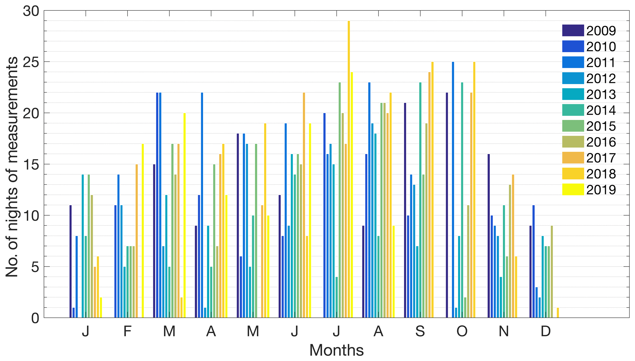
Figure 1 The total number of semi-clear nights with at least 30 min of profiles per month from 2009 through the middle of August 2019. Winter months have fewer measurements due to more cloud cover and precipitation. Most measurements are taken in the summer.

Figure 2 The monthly climatology for tropospheric water vapour from RALMO in units of specific humidity (g kg⁻¹). Contours for specific humidity are labelled in bold black. Dashed white lines are the average altitudes for each pressure level and are in units of metres. Larger amounts of water vapour are seen in the summer months due to higher temperatures. The lowest pressure is 250 hPa during the summer months. In the winter, the lowest pressure is 280 hPa due to the lower water vapour content. Higher water vapour content is shown in darker blue colours and lower water vapour content in lighter colours.

2.2 Radiosondes

2.2.1 GRUAN radiosondes

GCOS Reference Upper Air Network (GRUAN)-certified radiosondes are currently the highest-quality radiosonde data product available. These radiosondes have been well characterized and corrected for several biases (Dirksen et al., 2014). Unique to GRUAN radiosonde products is the calculation of measurement uncertainties as a function of altitude, which allows for better comparison between radiosondes and other instruments. The aerological station of MeteoSwiss in Payerne, Switzerland, has been launching Vaisala RS92 sondes biweekly at noon and midnight UTC since October 2011 to obtain GRUAN-certified profiles of temperature and humidity. Launches are co-located with RALMO. Unfortunately, not all of the radiosondes launched at the station from 2009 to 2018 were GRUAN-compliant or GRUAN-corrected; therefore, we were unable to calculate a GRUAN radiosonde climatology or use them for trends. GRUAN-certified sondes were used to calculate the lidar calibration constants in Appendix A as well as examine the uncertainty in the daily radiosondes (Hicks-Jalali et al., 2019).

2.2.2 Daily radiosondes

MeteoSwiss also launches an operational radiosonde every day at 11:00 and 23:00 UTC. The MeteoSwiss operational radiosonde time series uses multiple radiosonde types: the SRS400 (Martin et al., 2006; Morland et al., 2009; Brocard et al., 2013b) from 2009 to 2010, SRS-C34 from 2010 to January 2017, SRS-C50 from February 2017 to March 2018, and the Vaisala RS41 (Jensen et al., 2016) from March 2018 to present day. The C34 and C50 radiosondes are manufactured by MeteoLabor. The C34 uses a Sippican hygristor for humidity measurements, which is quoted to have an accuracy of 2 % relative humidity (RH) (Meteolabor, 2010); however, no public validation studies have been published. The C50 is the updated version of the C34; however, no public documentation exists on the C50 specifications. As these radiosondes are not GRUAN-certified, we do not use them to compare with the individual lidar profiles. However, we have compared their PWV measurements to those of the coincident GRUAN-processed RS92 radiosondes. We compared the operational sonde PWV measurements to coincident GRUAN PWV measurements and found an average difference of 0.8 %±3.7 % PWV between the two sets of sondes. The scatter in the radiosonde measurements did not change between the different types of radiosondes; therefore, we have not attempted any homogenizing between the different data sets. The average difference between the two sets of sondes was within the GRUAN uncertainty for PWV; therefore, we were comfortable using the operational sondes for PWV comparison with RALMO. We have also used the pressure measurements from these radiosondes to map the retrieved water vapour lidar altitude profiles onto a standard pressure grid.

3 A monthly tropospheric water vapour climatology for Switzerland

Climatologies are extremely useful as they provide a baseline for daily measurement comparison and can be used as a priori information for forecast modelling and reanalysis models. To that end, we have calculated a monthly water vapour climatology using the RALMO measurements for Payerne, Switzerland. A monthly climatology was chosen instead of a daily climatology due to the inability to retrieve enough coincident daily measurements to accurately represent a daily average.

A Raman lidar's native measurement grid is in altitude; however, models and satellites often work on pressure grids. Therefore, we have interpolated our final retrieved profiles onto a pressure grid to facilitate comparisons with other studies. The climatology data as a function of altitude and pressure have been made available via the Zenodo database (Hicks-Jalali et al., 2020). We interpolated each profile onto a standard pressure grid from 950 to 100 hPa using pressure and altitude data from the operational radiosondes launched at midnight UTC. When surface pressures are higher than 950 hPa, the measurements are extrapolated. No surface pressure measurements were higher than 960 hPa.

Once the lidar profiles have been interpolated, all profiles in a month which pass the cost threshold of 3.5 are averaged together and weighted based on their statistical uncertainties. Due to the cloud masking applied to each individual profile, it is possible that some altitude bins will use fewer measurements than others. We required each individual bin to have measurements from at least 5 different years, with at least three measurements per year to calculate a representative average state. This means that the minimum number of measurements is 15 per pressure bin. Figure 2 shows the resulting specific-humidity climatology with respect to pressure. The corresponding average altitudes for each pressure are shown as white contour lines.

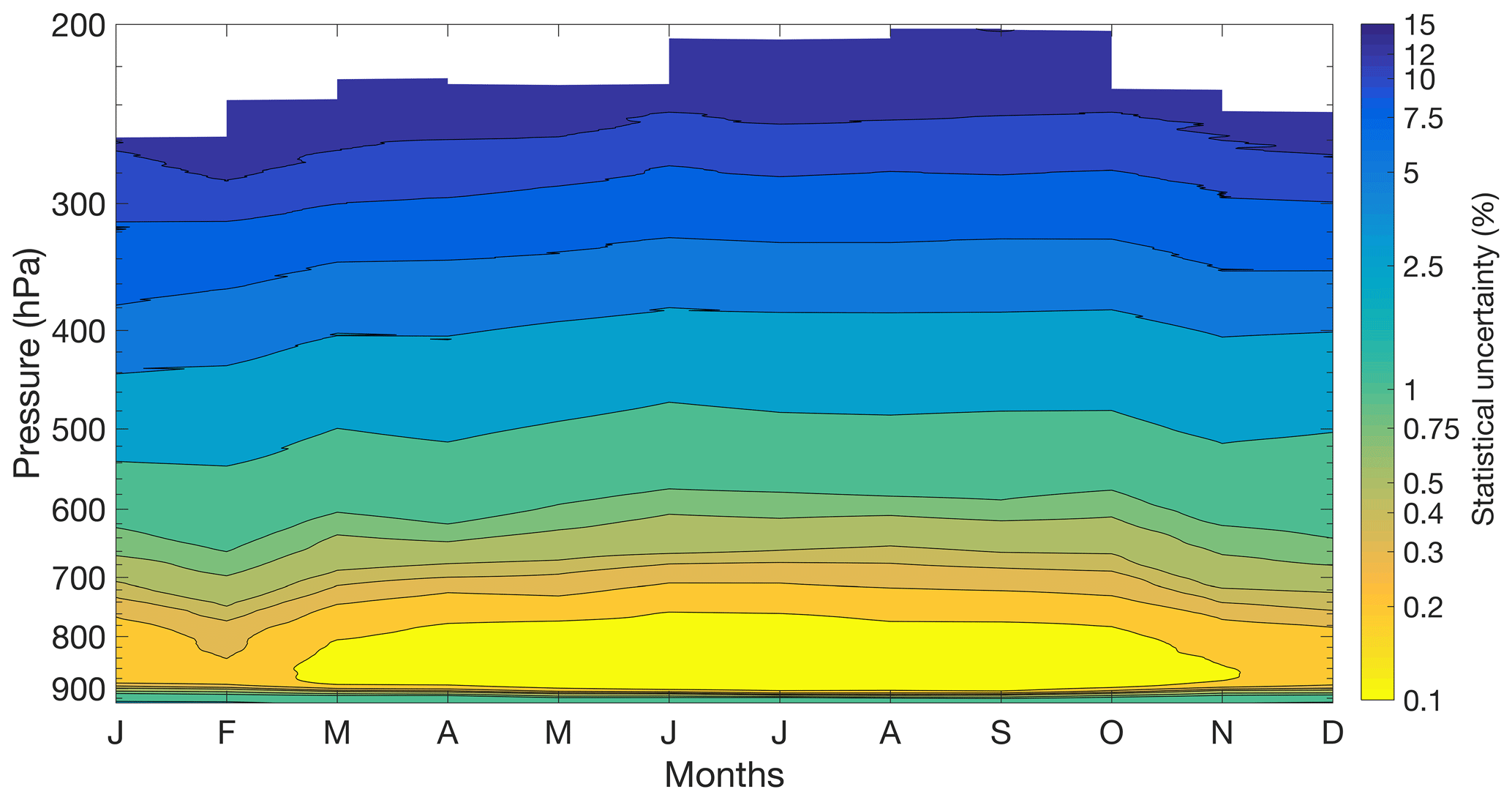
Figure 3 The average statistical uncertainties (represented as percentage of uncertainty) for each month as a function of pressure. The highest statistical uncertainty is 14 % of the water vapour mixing ratio between 275 and 250 hPa, or between 11 and 12 km.

The climatology shows the expected seasonal cycle for water vapour with high concentrations (darker blues) in the summer and lower concentrations in the winter. The spring months are slightly drier than the fall months, with specific-humidity values only starting to increase in April and high summer concentrations lasting through September. On average, the lidar is able to retrieve measurements consistently (at least 15 profiles per bin over 5 years) up to 280 hPa (roughly 10 km). However, in the summer months, the climatology reaches up to 250 hPa (roughly 12 km) due to higher lidar signal-to-noise ratios (SNRs) from the higher water vapour content.

The average statistical uncertainties for the climatology are consistent across all seasons, with the exception that the summer months and September show smaller uncertainties at lower altitudes due to their larger SNRs (Fig. 3). The average statistical uncertainties are calculated by taking the average of the uncertainties for all the profiles used in each month. The statistical uncertainties are presented as the uncertainty in the water vapour mixing ratio and not the uncertainty in specific humidity. The OEM retrieval is in units of water vapour mixing ratio, and while we have converted the final retrieval profiles to units of specific humidity, even at the highest concentrations of water vapour the difference between the two units is less than 2 %. Therefore, the uncertainties calculated for the water vapour mixing ratio are comparable to the uncertainties for the converted specific-humidity profile. The strength of the Raman lidar signal and the statistical uncertainty is dependent on the amount of water vapour present in the atmosphere. Therefore, high statistical uncertainties are associated with low specific-humidity levels. At high pressures, where more water vapour is present, such as in the boundary layer, the statistical uncertainty is less than 1 %. However, at lower pressures and near the tropopause, where water vapour quantities are low, the statistical uncertainties reach an average of 14 %. In the winter, when the air is drier, we see slightly higher uncertainties than in the summer at the same altitudes. At the surface, 82 % of the profiles used in this study have statistical uncertainties of less than 5 %, and 96 % of the profiles have statistical uncertainties less than 10 %. At 250 hPa, 77 % of the profiles have uncertainties lower than 20 %, while the remaining 23 % have uncertainties between 20 % and 25 %.

In this study we refer to the individual retrieval uncertainties in water vapour mixing ratio due to uncertainties in non-retrieved forward-model parameters as parameter uncertainties (Fig. 4). Parameter uncertainties are calculated via Gaussian uncertainty propagation for each retrieval parameter. Figure 4 shows the parameter uncertainties' effect on water vapour mixing ratio calculated for each retrieval, including the calibration constant, Ångstrom exponent, National Center for Environmental Prediction (NCEP) air density, aerosol extinction profile, overlap, and the Rayleigh cross-section. Details regarding the covariances of the system parameters can be found in Appendix 4B of Hicks-Jalali (2019). Every uncertainty profile used in the climatology is shown in dashed grey lines, and the average uncertainty for each component is the dashed black line. Note that systematic uncertainties are on a different height scale for the aerosol extinction profile and overlap components. This choice is because these forward-model parameters are also retrieval parameters for part of the profile. Overlap is retrieved from the ground to 400 hPa; therefore the uncertainty in overlap on the retrieved water vapour mixing ratio is only calculated above 400 hPa. The opposite situation occurs for the retrieved aerosol extinction; it is retrieved above 400 hPa, and therefore its uncertainty on the water vapour mixing ratio is only calculated below 400 hPa. The largest systematic uncertainty, which dominates the retrieval, is the 5 % calibration uncertainty. Sica and Haefele (2016) originally assigned a value of 5 %, which was later confirmed by the study conducted in Hicks-Jalali et al. (2019). The residuals of the smoothing spline fit to the combined calibration time series also showed an average of 5 % variation in the residuals (Appendix A). The second-largest component is the uncertainty due to the assumption of the aerosol Ångstrom exponent. The OEM retrieval assumes that the Ångstrom exponent does not change with altitude, which can cause larger uncertainties in clouds where our assumed value may not be appropriate. We used a mean climatological value of 1.5±0.5, which results in an average uncertainty on the order of 1 % in the water vapour mixing ratio. In 4 out of the 1300 nights used in this study, the uncertainties caused by the uncertainty in the Ångstrom exponent were larger than 5 % due to the Ångstrom exponent choice being a poor fit in a persistent cloud. The uncertainty due to NCEP model air density is slightly higher than the Ångstrom exponent uncertainty at altitudes below 2 km but with an average uncertainty of around 0.25 % for all altitudes. All other systematic uncertainties, including extinction, overlap, and the Rayleigh cross-section, are less than 0.1 %. However, the Rayleigh cross-section uncertainties also had four nights which exhibited uncertainties larger than 0.5 %. The major improvement to the water vapour retrieval since Sica and Haefele (2016) is the retrieval of overlap from the surface to 6 km (if there are no clouds below 6 km). In Sica and Haefele (2016), overlap was not a retrieval parameter and added another 7 %–10 % uncertainty below 3 km.

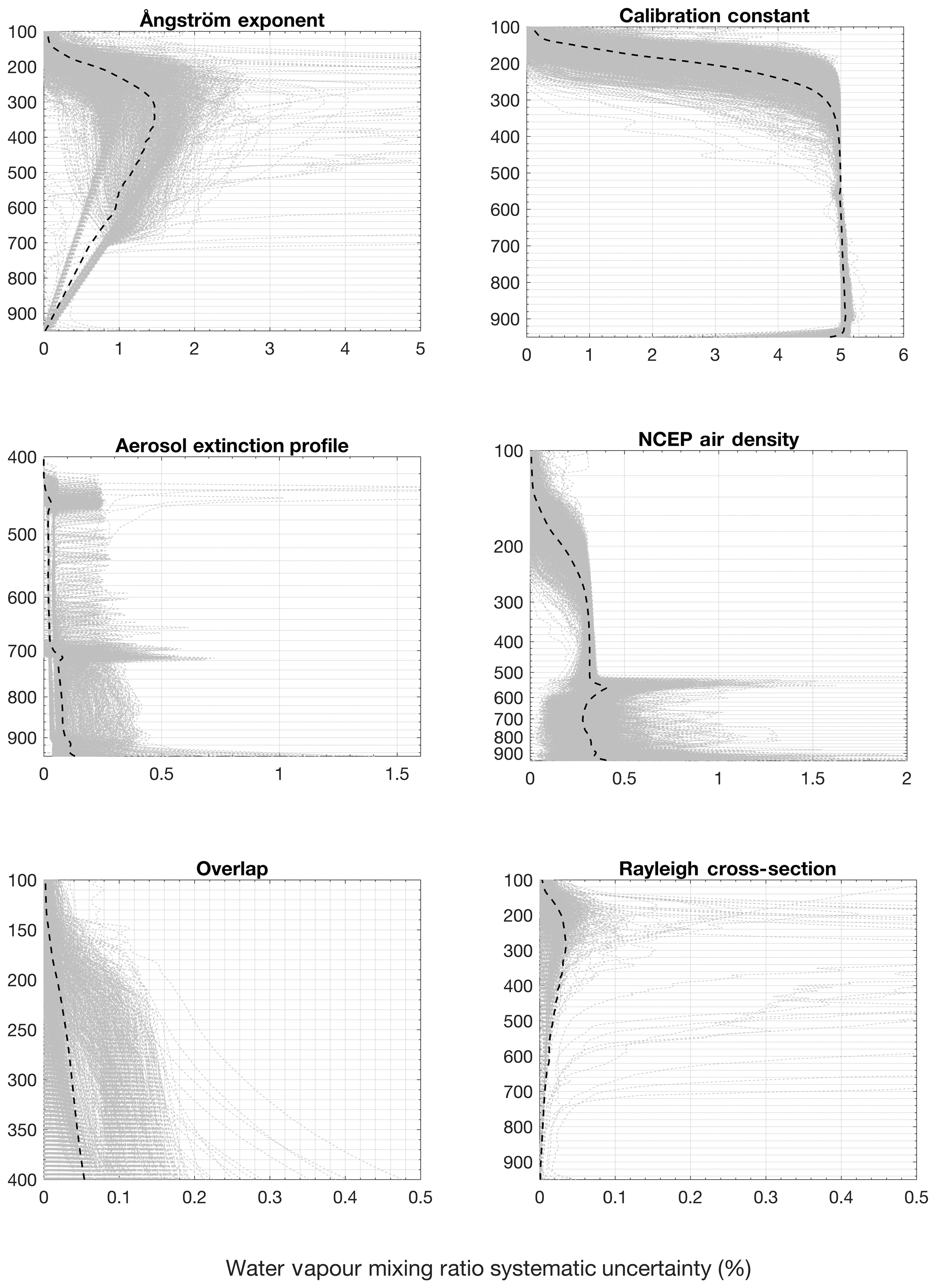
Figure 4 The water vapour mixing ratio systematic uncertainty budget for each night used in the water vapour climatology (dashed grey lines) and the average uncertainty contribution from each component (dashed black line). The largest contributors are the Ångstrom exponent and the calibration constant. A total of 4 nights out of 1300 had Ångstrom exponent uncertainties larger than 5 % due to our assumed value not fitting with persistent clouds. The average uncertainty contribution from the NCEP air density is 0.25 %. All other uncertainties contribute less than 0.1 % on average.

We also compared the lidar PWV measurements to the PWV column from the Payerne daily radiosondes during the same time period as the height-resolved climatology. The radiosonde measurements are systematically larger than the lidar measurements, likely due to the fact that the lidar is not able to take measurements in the first 100 m from the surface. The lidar PWV climatology agrees with the operational radiosonde PWV climatology within their respective uncertainties (Fig. 5). The uncertainties for the climatology were calculated using the standard deviation of all measurements in 1 month.

Figure 5 The PWV climatology of both the lidar and the operational radiosondes. The error bars are the 1σ standard deviation of all of the measurements in each month. The climatology was calculated using the same dates for both the radiosonde and the lidar measurements.

The PWV climatology shows the same behaviour as the profile climatology already shown in Fig. 2, with the largest amount of water vapour in the summer months and smallest amounts in the winter months.

3.1 Geophysical variability

Water vapour concentrations change by up to 4 orders of magnitude through the troposphere. The troposphere is also a region of many dynamic processes, including the hydrologic cycle as well as general global circulation. These processes have a direct impact on water vapour variability and make it difficult to measure. The abundance of measurements used in this study makes it possible to estimate water vapour's variability as a function of altitude. The geophysical variability (σ_geo(z)) of the specific humidity can be estimated by taking the standard deviation of all profiles in 1 month (σ_w(z)) and removing the measurement variability, which is dominated by the statistical uncertainty (σ_stat(z); Eq. (3); Argall and Sica, 2007). The remaining variability should then be physical in nature.

$$\begin{array}{}\text{(3)}& {\mathit{\sigma }}_{\mathrm{geo}}^{\mathrm{2}}\left(z\right)=\mathrm{100}{\displaystyle \frac{\left({\mathit{\sigma }}_{\mathrm{w}}^{\mathrm{2}}\left(z\right)-{\mathit{\sigma }}_{\mathrm{stat}}^{\mathrm{2}}\left(z\right)\right)}{\langle q\left(z\right){\rangle }^{\mathrm{2}}}}\end{array}$$

The percentage of geophysical variability for water vapour was calculated using Eq. (3), in which ${\mathit{\sigma }}_{\mathrm{w}}^{\mathrm{2}}\left(z\right)$ is the variance of all monthly profiles, ${\mathit{\sigma }}_{\mathrm{stat}}^{\mathrm{2}}\left(z\right)$ is the average of the statistical uncertainty variances of the retrievals, and 〈q(z)〉 is the climatology. Figure 6 is then the geophysical variability in units of percentage of variability from the mean state.

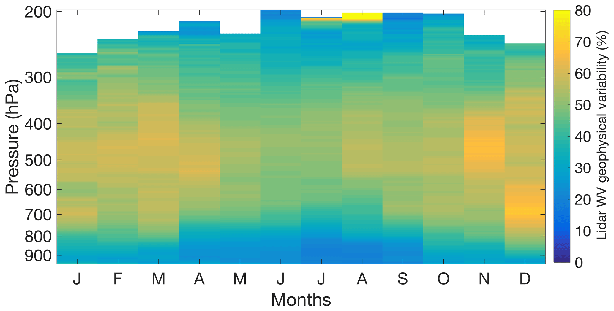
Figure 6 The monthly geophysical variability of water vapour measured by RALMO as a function of pressure. The largest amount of variability can be seen in the free troposphere between 600 and 400 hPa in the summer and from 800 to 450 hPa in the winter.

The smallest percentage of variability is in the boundary layer, typically in the summer. However, as this is a nighttime and primarily clear-weather climatology, the boundary layer should be stratified and either neutral or stable at these times. Therefore, Fig. 6 would represent the variability of the boundary layer during nighttime and primarily high-pressure conditions.

Above the boundary layer, from 700 hPa in the winter, spring, and fall and up to 350 hPa, there is much higher variability present. The largest variabilities of 60 % or higher are located between 550 and 400 hPa during the spring and fall and between 750 and 600 hPa in December. The latter region in December is likely due to sampling bias since December had half the measurements as the summer months. However, the high-variability regions between 600 and 400 hPa are interesting and could represent dynamic processes at work. The region from 600 to 400 hPa is a region of active mixing of air from the upper troposphere or stratosphere and the surface. Simultaneously, planetary waves transport air horizontally from different air masses at these heights. Therefore, we would expect the region from 600 to 400 hPa to exhibit a high amount of variability.

We compared the lidar-measured geophysical variability to the water vapour geophysical variability measured by the operational radiosondes. All available daytime and nighttime operational radiosondes were used to calculate the geophysical variability. The total value of the percentage of geophysical variability is only an estimate because we do not know the uncertainty of the daily radiosonde's humidity measurements. The maximum uncertainty reported by the GRUAN radiosondes in the troposphere is around 10 % of the mixing ratio measured. Therefore, we assume a constant uncertainty in the operational radiosonde measurements of 10 %, although this would be a lower limit of the uncertainty of the routine sondes because they have not been corrected. The variability is then calculated in the same way as for the lidar (Fig. 7).

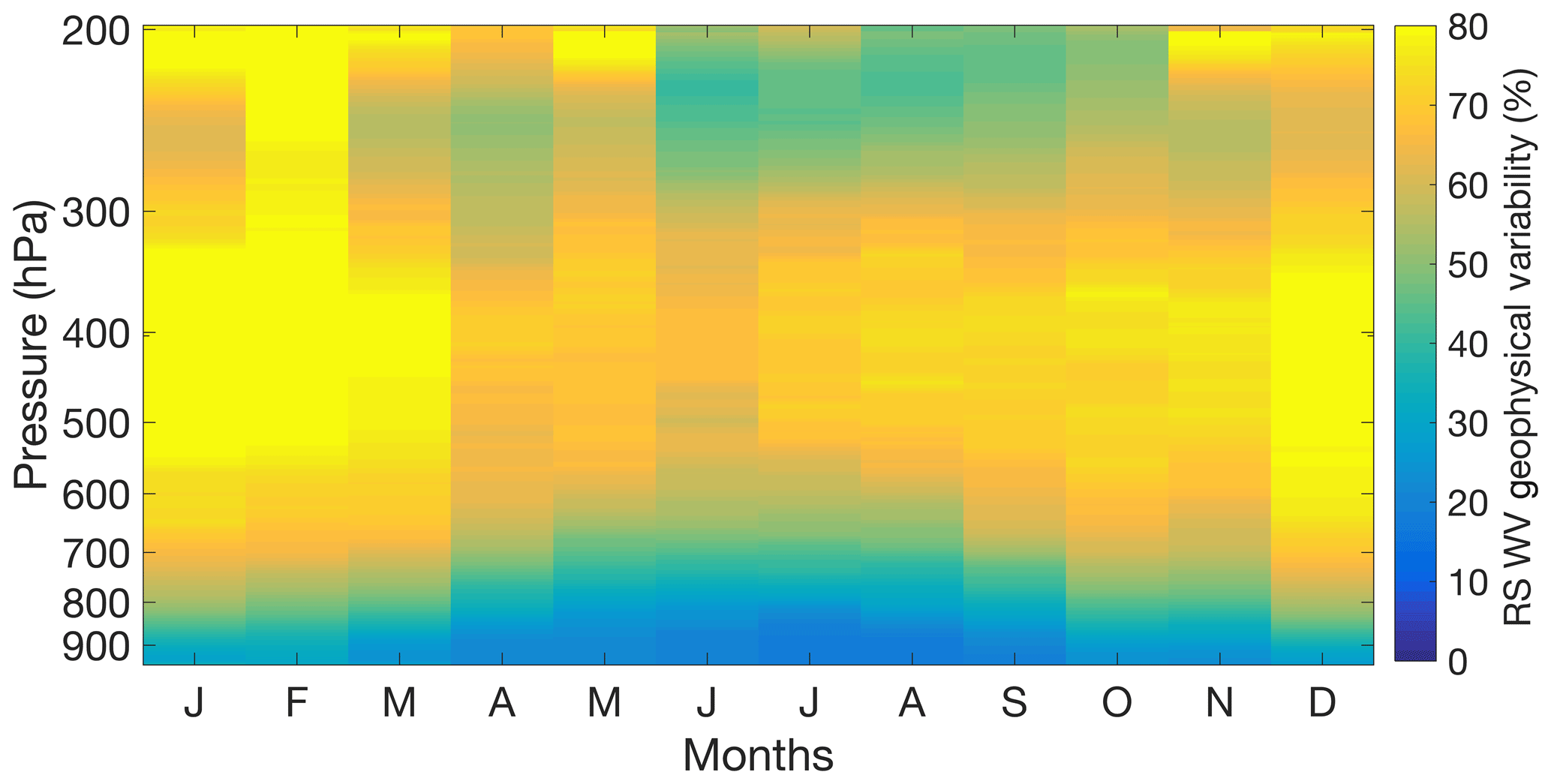
Figure 7 The water vapour geophysical variability estimated using all available daytime and nighttime operational radiosondes as a percentage and function of pressure. The radiosondes see the same behaviour as the lidar, and the distribution of the variability is the same, although the magnitude is generally 20 % larger. The larger magnitude is possibly due to the underestimation of the daily radiosonde uncertainties.

The radiosondes measure similar behaviour in the variability to the lidar; however, the magnitude of the variability is roughly 20 % larger than the lidar's. As discussed earlier, half of this difference is likely due to underestimating the uncertainty in the operational radiosondes. However, it could partially be due to the fact that more measurements are available from the radiosonde than from the lidar. When comparing November and December profiles, it can be seen that the regions of large lidar variability in November and December are likely due to sampling bias and not physical processes. However, it is encouraging to note that the same physical structure is seen in both instruments. This result would suggest that the large variability in the troposphere is not due to clouds or layers affecting the climatology but likely due to the increased mixing of air between 600 and 400 hPa in the summer and between 700 and 450 hPa in the winter. In high-pressure systems, the air from the stratosphere and high regions of the troposphere converge, which causes air to subside at the surface (Holton, 2004). The colder air in the stratosphere and lower troposphere is usually drier. This exchange of moist air and dry air in the free troposphere could explain the large variability. It is interesting to see that adding the daytime sondes to the variability calculation does not change the overall behaviour of the water vapour in the troposphere. We explored looking at the difference between the variability including daytime sondes and not including the sondes and found almost no difference in the variability when the daytime sondes were added. The radiosondes and the lidar measure more variability in the winter months than in the summer months. European winter weather is highly influenced by the polar jet stream. An increase in the variability of water vapour during these months could be caused by an increase in the exchange of air between the Arctic and the mid-latitudes.

4 Deriving trends

There have been several tropospheric water vapour trend studies conducted over the course of the last few decades, only a few of which are cited here (Hense et al., 1988; Ross and Elliot, 1996, 2001; Morland et al., 2009). Whiteman et al. (2011a) investigated the potential for water vapour Raman lidar trend calculations and carefully estimated the thresholds needed to calculate statistically significant trends in the upper troposphere. They found that with no statistical uncertainty, one would need between 10 and 12 years of daily measurements to calculate trends at 200 hPa due to water vapour's naturally large variability at that pressure. We have 11.5 years of measurements and are therefore in the realm of possible detection at the 95 % level; however, whether or not we can detect trends depends on the variability of the atmosphere at the levels we choose and the magnitude of the trend itself. As we show, the variability of the atmosphere in the free troposphere will determine our ability to detect trends at the 95 % level. According to Weatherhead et al. (1998), trends of at least 5 % per decade should be calculable in 10 years, provided the standard deviation of the noise in the trend residuals is less than 6 %, and the autocorrelation of the trend fit residuals is less than 0.4 (Table 1 of Weatherhead et al., 1998). Therefore, the lowest pressure at which we should be able to calculate trends of at least 5 % is around 350 hPa (11 km), provided the autocorrelation is small, and we have relatively little noise in our trend residuals.

4.1 Trend estimate methodology

The bootstrap method of Gardiner et al. (2008) makes use of a least squares regression for a model which includes both the linear trend and the annual and semi-annual oscillations via a Fourier function (Eq. 4):

$$\begin{array}{}\text{(4)}& \begin{array}{rl}f(t,a,b)& =at+b_{\mathrm{0}}+b_{\mathrm{1}}\cos \left(\mathrm{2}\mathit{\pi }t\right)+b_{\mathrm{2}}\sin \left(\mathrm{2}\mathit{\pi }t\right)\\ & +b_{\mathrm{3}}\cos \left(\mathrm{4}\mathit{\pi }t\right)+b_{\mathrm{4}}\sin \left(\mathrm{4}\mathit{\pi }t\right)\\ & +b_{\mathrm{5}}\cos \left(\mathrm{6}\mathit{\pi }t\right)+b_{\mathrm{6}}\sin \left(\mathrm{6}\mathit{\pi }t\right),\end{array}\end{array}$$

where a is the trend in units of either grams per kilogram per year or millimetres per year, the vector b is comprised of all the seasonal variation coefficients (b_n, n=0, 1, …6) as well as the offset (b₀), and t is time. Gardiner et al. (2008) found that, for their study, it was not necessary to continue beyond the third order of the Fourier series as doing so no longer decreased the root mean square (RMS) of the residuals. We also found no difference in the residual RMS by adding terms beyond the third order in the Fourier series. Indeed, the third order could probably have been removed as well; however, we have kept it to maintain consistency with other studies.

We calculated trends using monthly averages of nightly averaged measurements from RALMO as well as the nightly radiosondes. Monthly averages were used to reduce the autocorrelation of the measurements and increase the statistical significance of the trends. The statistical significance of the trends was determined by using the uncertainty equation from Weatherhead et al. (1998), which includes the autocorrelation coefficient of the residuals:

$$\begin{array}{}\text{(5)}& {\mathit{\sigma }}_{\mathrm{a}}={\displaystyle \frac{{\mathit{\sigma }}_N}{n^{\mathrm{3}/\mathrm{2}}}}\sqrt{{\displaystyle \frac{\mathrm{1}+\mathit{\varphi }}{\mathrm{1}-\mathit{\varphi }}}}.\end{array}$$

The uncertainty of the trend (σ_a) is determined from σ_N, the standard deviation of the residuals from the least squares fit; n, the number of years of measurements (in our case 11.5); and ϕ, the autocorrelation coefficient at lag 1. All uncertainties presented in this study are 2σ_a to determine if the corresponding trend is statistically significant at the 95 % level.

As shown in Fig. 1, some months of data are missing from the full time series. However, there were no successive gaps in the monthly averaged time series. We linearly interpolated the monthly average time series before calculating the trend to fill the six gaps in the missing months and to calculate meaningful autocorrelation coefficients.

4.2 Precipitable water vapour trends

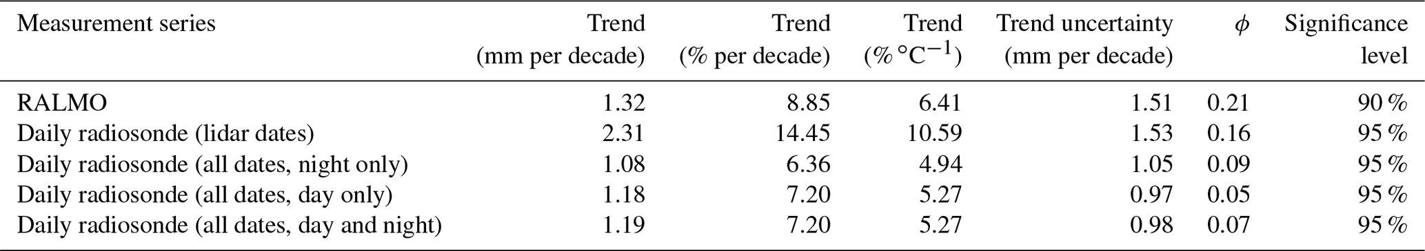
We first calculated tropospheric precipitable water vapour (PWV) trends using RALMO and the daily radiosonde measurements to compare with the majority of previous studies where height-resolved measurements were not available. Precipitable water vapour values were calculated by integrating water vapour densities between the daily station surface pressure as measured by the daily radiosonde and 280 hPa to maintain the same pressure range over the entire year. Table 1 shows the value of the trends for the 30 d averaged RALMO and daily radiosonde nighttime measurements from January 2009 to August 2019. The PWV measurements, the function fits, and the trend lines are shown in Fig. 8. We calculated four radiosonde trends to compare with the RALMO PWV trend. The first two methods used only nighttime data, but the first limited the data to the same nights as the radiosonde, and the second used all available nighttime radiosondes. They are shown in rows 1 and 2 of Table 1, respectively. The difference between the two nighttime radiosonde trend methods could represent the bias from using only semi-clear nights during clement weather. However, the bias between the two radiosonde nighttime trends is more likely caused by the number of points used in each trend and the uncertainty in the radiosonde measurements. Roughly 25 % of the possible nights are used in the trend analysis for the coincident lidar dates, and as the radiosondes do have a larger and non-characterized uncertainty, it is more likely that the large trend value is due to a larger scatter in the radiosonde measurements. Given that the lidar trend is much closer to the radiosonde trends which use all available nights, including the radiosonde trends calculated using daytime and nighttime measurements, the large radiosonde trend using only nights consecutive with the lidar is more likely due to random error and not a difference in weather. We also calculated daytime radiosonde trends using all available daytime measurements as well as a combined trend using all available daytime and nighttime measurements (rows 3 and 4 of Table 1). The daytime radiosonde trends differ from the nighttime radiosonde trend using all available nights by 0.1 mm per decade, and they agree within their 1σ uncertainties.

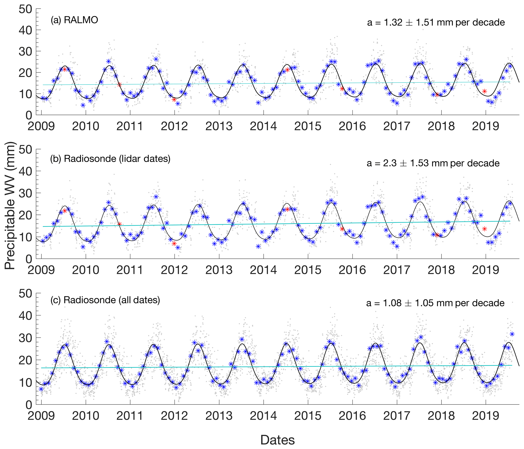
Figure 8 The nighttime precipitable water vapour measurements taken by RALMO and the daily radiosondes. For all subplots, the nightly measurements are the grey dots, 30 d averages are the blue stars with interpolated points in red, the fitted function is in black, and the trend line is in light blue. (a) RALMO PWV measurements, (b) radiosonde PWV measurements on coincident dates with lidar measurements, (c) radiosonde PWV measurements for all available dates.

Table 1 Table of precipitable water vapour trends calculated using RALMO and daily radiosonde monthly averaged measurements from January 2009 to August 2019. Trends are presented in units of millimetre per decade (mm per decade), per cent change from the mean per decade (% per decade), and per cent change in water vapour per degree Celsius (% ^∘C⁻¹). The trend values in column 3 were calculated by dividing the water vapour trend in column 2 by the surface temperature trend of 1.38±1.41 ^∘C per decade. Trend uncertainties are 2σ_a values, in units of millimetres per decade, and are calculated using Eq. (5).

The lidar and radiosonde precipitable water vapour trends have varying levels of significance. The RALMO trend is significant above 90 %, while the radiosonde trends are significant above 95 % (Table 1). The trend calculated using all available nighttime radiosonde measurements is slightly smaller than the RALMO PWV trend but slightly larger than previously calculated trends for Payerne and the region (Morland et al., 2009; Wang et al., 2016; Nyeki et al., 2019).

The Clausius–Clapeyron relationship suggests that the water vapour in the atmosphere should increase by roughly 7.5 % per 1 ^∘C or more depending on the initial temperature (Held and Soden, 2000). Therefore, such large PWV changes should be correlated with proportionally large increases in temperature. We used the temperature measurements at 500 m (950 hPa) a.s.l. from the daily radiosonde to compare with the lidar water vapour trend because the lowest-available measurements are at 550 m. We assume that the lidar PWV measurements should correspond best with the temperatures at that altitude. The same nights used in the lidar and radiosonde water vapour trend analysis were used for the radiosonde temperature measurements. The 950 hPa temperature trend was statistically significant at 95 %, with a slope of 1.38±1.41 ^∘C per decade. The temperature trend we measure is larger than that measured by Morland et al. (2009) and Nyeki et al. (2019). However, the per cent change in water vapour per degree Celsius for all PWV trend values is between 5 % and 10 %, which is consistent with the expected change assuming that relative humidity is conserved. The differences between our temperature trend measurements and other studies is discussed further in Sect. 5.

4.3 Height-resolved trends

Here we show height-resolved water vapour trends measured at 11 layers of the troposphere from 950 to 250 hPa. Each layer is an average of measurements from ±10 hPa from the centre (e.g. measurements at 900 hPa are an average between 890 and 910 hPa). The layers were averaged to reduce the variability due to choosing a single pressure level. We calculated the trend for each layer using monthly averages of the time series. We calculated the specific-humidity height-resolved trends using the same bootstrapping method that was used for the PWV trends.

An example of the trend at 800 hPa is shown in Fig. 9. The blue asterisks are the monthly averages, with the interpolated points shown in red. The nightly points are shown in light grey. The trend and seasonal fit are in light blue and black, respectively.

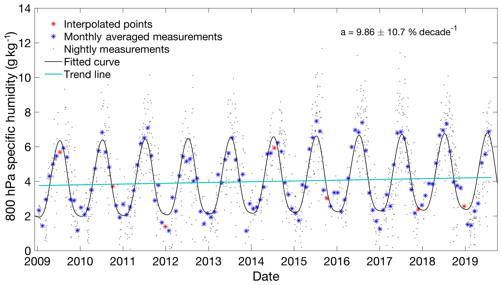
Figure 9 An example lidar specific-humidity trend at a fixed pressure level of 800 hPa showing the seasonal fit (black) and the linear trend line (light blue). Nightly measurements are in grey, and monthly averages are blue asterisks with the seven interpolated monthly points in red. The trend is calculated over the series, which includes the interpolated points.

The trends at each layer are shown in Table 2. The trend at 950 hPa is statistically significant at the 95 % level, while trends at 800, 700, 600, and 350 are significant at the 90 % level. The trend at 400 hPa is statistically significant at the 80 % level. The rest of the trends have significance levels of less than 80 %. The trends in Table 2 are presented in absolute units per decade, per cent change from the mean per decade and per cent change from the mean per degree Celsius. The uncertainties are presented as 2σ_a in units of per cent change from the mean per decade. All trends were positive but varied between 3 % and 16 % per decade depending on the layer. The trend at 950 hPa is statistically significant, but the noise in the residuals is less than the noise at 900 hPa.

Table 2 Table of RALMO specific-humidity trend calculations for each pressure layer. The first column is the specific-humidity trend in units of grams per kilogram per decade, the second column is the specific-humidity trend in per cent per decade, the third column is the specific-humidity trend in units of per cent change per degree Celsius. The fourth and fifth columns are the uncertainties of the trend in units of per cent per decade and the autocorrelation value at lag 1.

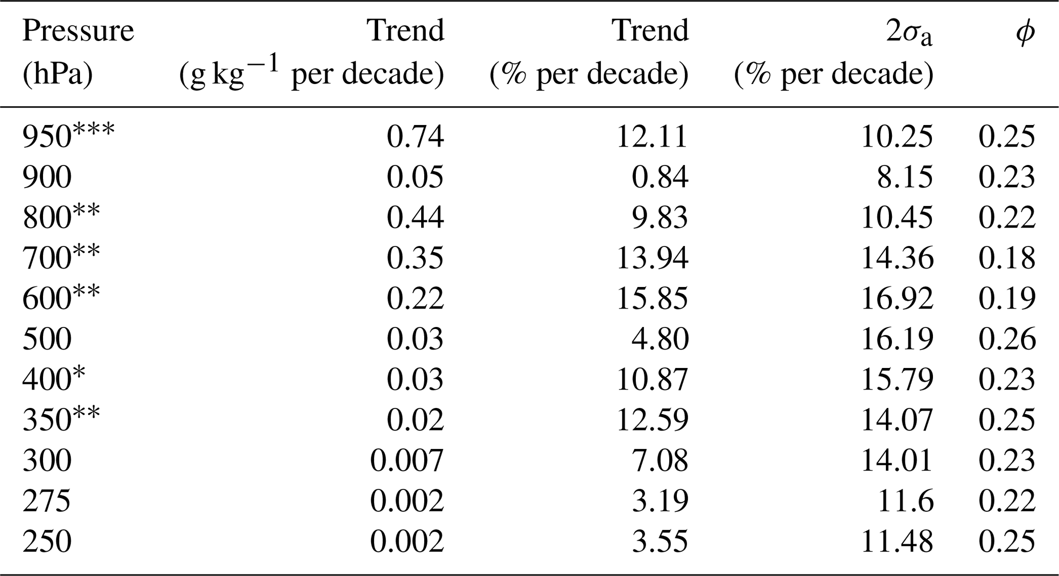
To calculate the change in the specific humidity per degree Celsius, we also calculated layered temperature trends using the daily radiosondes. The radiosonde temperature measurements were also averaged over the same pressure ranges as the specific-humidity trends and averaged monthly. The temperature trends are presented in Table 3. All available nights were used to calculate the temperature trends. We found all temperature trends to be positive, with the largest being 1.38 ^∘C per decade at 950 hPa. All of the temperature trends were statistically significant at the 95 % level. The temperature trends are larger by about 0.4–0.8 ^∘C per decade than what was reported in Morland et al. (2009) and Brocard et al. (2013a). Interestingly, dividing the height-resolved water vapour trends by the temperature trends does not produce the expected 7 % ^∘C⁻¹ relationship which was seen in the precipitable water vapour trends, with the exception of the trend at 950, 300, and 250 hPa. Instead, we see increases on the order of 10 %–17 % ^∘C⁻¹ between 800 and 300 hPa. The rest of the layers present humidity changes with temperature that would indicate that relative humidity may not be conserved at the individual layers. The PWV trends are likely dominated by the surface water vapour trend, which is why PWV and 950 hPa trends are similar.

Table 3 Table of temperature trend calculations for each pressure layer using the operational radiosondes. The second column is the temperature trend in units of degrees per decade, the third column is the 2σ_a trend uncertainty in units of degrees per decade, the fourth column is the autocorrelation coefficient at lag 1, and the fifth column is the per cent change in specific humidity per degree Celsius.

Trends marked with a ^*, ${}^{**}$, and ${}^{***}$ are statistically significant at the 80 %, 90 %, and 95 % level respectively.

5 Discussion

We have calculated a lidar climatology of the water vapour distribution above Payerne, Switzerland, using measurements from 2009 to 2019 from the RALMO lidar as well as a precipitable water vapour climatology. RALMO is one of a few lidars which has produced a published high-vertical-resolution water vapour climatology of the troposphere with 11.5 years of consistent measurements. The climatology in Hadad et al. (2018; H2018) is the only other published ground-based Raman lidar climatology (410 m; 45.77^∘ N, 2.96^∘ E). The climatology in H2018 shows a wet bias of roughly 2 g kg⁻¹ at the surface in September and October compared to RALMO. This difference is likely due to the fact that they only have 6 years of measurements, from 2010 to 2016. The remaining months show good agreement between the RALMO and H2018 lidar climatologies. Our RALMO climatology agrees very well with the H2018 Atmospheric Infrared Sounder (AIRS) on the Earth Observing System (EOS) climatology, which had more measurements from 2002 to 2017. The AIRS water vapour climatology was calculated for the 100 km radius around Cezeaux, France. The differences between the AIRS and RALMO climatologies are less than 1 g kg⁻¹.

H2018 also calculate a standard deviation for their climatology. However, it is important to note that this is not the same as the geophysical variability that we have calculated as they do not subtract the variability due to their measurement noise. Additionally, they do not look at the relative variability but the absolute. They show large standard deviations in the boundary layer and lower troposphere and very small standard deviations in the upper troposphere. However, dividing their standard deviation by their climatology produces variability measurements comparable to ours of around 20 % to 30 % in the boundary layer and between 40 % and 80 % in the free troposphere. H2018 states that they see more variability in the boundary layer; however, we would argue that this is because they are looking at the absolute value of the variability and not the percentage. The free troposphere actually has larger variability since it has much smaller concentrations of water vapour. In summary, both the H2018 and our variabilities are consistent with each other.

The RALMO climatology is a nighttime and clear-sky-only climatology. The AIRS climatology in H2018 is not cloud-filtered (or at least no mention is made of any cloud filtering), appears to use both day and night measurements, and differs from the RALMO climatology by less than 1 g kg⁻¹. The question is whether or not a nighttime climatology for Payerne can serve as a true representation of the average state. Morland et al. (2009) and Hocke et al. (2017) calculated the diurnal PWV cycle for Bern using the Tropospheric Water Vapour Radiometer (TROWARA) instrument and Global Navigation Satellite System (GNSS) measurements. Hocke et al. (2017) found that the average PWV diurnal amplitude was 2 % of the monthly mean. In other words, the total water vapour content changes by 2 % on average over the course of the day. The maximum change in water vapour was 4 % over the course of the day in June, and the minimum was less than 1 % in the winter months. While PWV cannot accurately represent the changes at individual layers, it does serve to show that as a whole the amount of water vapour does not change significantly over the course of the day. Perhaps the more important fact is that the phase of the diurnal cycle is such that the maximum amount of water vapour peaks around 20:00 LST and then decreases to reach a minimum at 08:00 LST the next morning. This would suggest that the average nighttime profile over a month is probably a good representation of the average water vapour content, and therefore a nighttime-only water vapour climatology is probably representative of the average water vapour content. It is important to note that this is the case for Payerne but would not necessarily apply to other locations.

Most water vapour trend studies of the troposphere focus on PWV measurements or surface humidity measurements. To compare with the literature, we also calculated precipitable water vapour trends using both RALMO and operational radiosonde measurements and found statistically significant trends of 1.3±1.53 mm per decade (8.8 % per decade, 90 % significant) and 2.3±1.51 mm per decade (14.4 % per decade, 95 % significant). These trends are larger than those calculated previously in Switzerland by Morland et al. (2009) and Hocke et al. (2011). The nighttime trends of Morland et al. (2009) were all positive, ranging between 0.3 and 0.9 mm per decade with uncertainties between 0.3 and 0.6 mm per decade depending on the instrument. The midnight radiosonde trend of Morland et al. (2009) using measurements from the surface to 200 hPa was 0.87±0.46 mm per decade and was statistically significant at 90 %. Hocke et al. (2011) found no trends in water vapour using microwave radiometer PWV measurements from 2004 to 2009. Nyeki et al. (2019) measured temperature and PWV trends from four locations in Switzerland, including the Payerne and Jungfraujoch research stations, with GPS measurements from 1996 to 2015. They calculated statistically significant (90 %) PWV trends at Payerne of 1.03 mm per decade during cloud-free conditions using Sen's slope method. Interestingly, the all-sky (cloudy and clear) condition trend produced a smaller trend value of 0.80 mm per decade (90 % significance). We also saw a similar drop in trend magnitude when including all-sky conditions in the radiosonde PWV trend with a change in trend value from 1.34±1.51 mm per decade to 1.08±1.05 mm per decade. Bernet et al. (2019) have published an update to the Nyeki et al. (2019) GNSS PWV trends and the Morland et al. (2009) TROWARA PWV trends using measurements from 1995 to 2018. They used Payerne GNSS measurements to calculate a PWV trend of 1.14±0.93 mm per decade, or 7.3±5.3  % per decade, which is statistically significant at 95 %. Their GNSS trend used all-weather and both night and day measurements. Their PWV trend calculation is consistent with the RALMO and radiosonde trends at the 1σ level.

We have discussed the clear-sky bias in our lidar PWV trends and found no statistically significant difference between the trends using all-weather measurements and our clear-sky-only PWV trends. The nighttime bias in the RALMO data set must also be discussed in comparison with the other literature and our radiosonde trends. We have calculated a statistically significant daytime-only PWV trend using the operational radiosondes with a magnitude of 1.19±0.99 mm per decade. We also calculated a mixed PWV trend using both daytime and nighttime measurements, which was also 1.18±0.97 mm per decade. The nighttime-only radiosonde trend is 0.1 mm per decade smaller than the daytime-only trend, and the RALMO trend is 0.14 mm per decade larger than the daytime trend. The GNSS trend calculated by Bernet et al. (2019) uses both daytime and nighttime measurements and agrees with our radiosonde trend, which uses both day and night measurements. The trend of Bernet et al. (2019) is also not statistically significant from the RALMO PWV trend at the 1σ level. Based on these results, we do not detect a bias using only nighttime measurements. While there may be a difference in the daytime and nighttime trends, it would be difficult to detect with such a short time series. Hocke et al. (2017) calculated an average PWV diurnal cycle amplitude of 2 % for Switzerland. Therefore, it would probably take a very long time series with very low scatter in the residuals to significantly detect a difference between day and night trends.

The PWV trends over the last 20 years have been increasing. One reason for the increase in the trends could be caused by a corresponding increase in the surface temperature trend over the same time period. We calculated a surface temperature trend with the Payerne daily radiosonde measurements from 2009 to 2019 of 1.38±1.41 ^∘C per decade. The MeteoSwiss 2017 Klimareport (MS2017; Bundesamt für Meteorologie und Klimatologie, 2017) reported an average surface temperature trend over Switzerland of 0.34 ^∘C per decade from 1961 to 2017, which was strongly significant. However, a steeper increase in temperature can clearly be seen in Fig. 4.1 of MS2017 for the period of 2009–2017, which would correspond with our larger trend value. Additionally, the MS2017 trend is for all of Switzerland, not just for Payerne. Nyeki et al. (2019) report a surface temperature trend of 0.79 ^∘C per decade (90 % significant) during cloud-free conditions and a trend of 0.59 ^∘C per decade (90 % significant) during all-sky conditions at Payerne using measurements from 1996 to 2015. The last 4 years have included 3 of the warmest years on record for Europe, which may have contributed to the increase in our temperature trends with respect to those of Nyeki et al. (2019; Copernicus Climate Change Service, 2019).

Brocard et al. (2013a) conducted a detailed study of height-resolved temperature trends and found several break points in Payerne temperature trends. While the temperature in the troposphere increased by 0.64 ^∘C from 1980 to 2000, the temperature trend decreased to almost zero from 2000 to 2010. Therefore, measurements which include the time period from 2000 to 2010 will likely have smaller trend values. The temperature trend appears to have increased again after 2010, but it is not possible with our measurements to determine the most recent break point. Despite the fact that the temperature trends differ between our studies, we measure water vapour trends close to the expected value of 7 % per degree Celsius. Therefore, the current PWV trends measured by RALMO and the operational radiosondes appear reasonable.

There are very few studies of height-resolved water vapour trends over the last few decades. Most tropospheric water vapour studies focus on surface or total column changes, with a couple including trends at 850 hPa (H2018; Serreze et al., 2012). While the majority of water vapour resides in the bottom 3 km, it is still of high importance to characterize and understand water vapour's behaviour throughout the troposphere. Height-resolved water vapour trends would benefit climate and forecast models. Additionally, Raghuraman et al. (2019) suggest that different height regions in the troposphere contribute unequally to the greenhouse effect. Their study showed that the middle tropospheric water vapour contributed the most to the water vapour component in the greenhouse effect. Lidars are well suited to height-resolved trend measurements, and the authors hope that this is the first of many similar studies which will appear over the next few years. We can compare our surface specific-humidity trends to the surface water vapour trends measured in Nyeki et al. (2019). They measured statistically significant surface specific-humidity trends in Payerne during cloud-free conditions of 0.18 and 0.23 g kg⁻¹ (depending on the method). We measured surface specific-humidity trends of 0.74±0.46 g kg⁻¹. Both studies detected trends which agree with the assumption of conservation of relative humidity, with Nyeki et al. (2019) detecting a change of 6 % ^∘C⁻¹ and RALMO detecting a change of 8.8±10.2 % ^∘C⁻¹. The difference between the two surface trends is likely due to the difference in temperature trend and the time period being used; however, when converting the trends to per cent per degree Celsius, the uncertainties in our surface trend encompass the Nyeki et al. (2019) surface trend value and the differences are not significant. We can also use the Jungfraujoch trends of Nyeki et al. (2019) trends to compare with our 700 and 600 hPa specific-humidity and temperature trends. The Jungfraujoch Observatory is at 3580 m, or about 650 hPa. The Nyeki Jungfraujoch cloud-free specific-humidity trend is 0.19 g kg⁻¹ per decade, while RALMO's trends at 700 and 600 hPa are 0.35±0.36 and 0.22±0.24 g kg⁻¹ per decade. The trends are the same within their respective 1σ_a uncertainties. Interestingly, neither our trends nor the Jungfraujoch trends of Nyeki et al. (2019) conform to the hypothesis that relative humidity is conserved. Both humidity trends with respect to temperature are at or above 14 % ^∘C⁻¹; however, they are not statistically significant above 95 % in those units. The relative humidity may be conserved over the troposphere or at the surface but not in individual layers. Raghuraman et al. (2019) recently tested the assumption of the conservation of relative humidity in a changing climate and found that in small geographical regions, relative humidity may not be conserved over time. However, globally, relative humidity is generally conserved. Height-resolved relative-humidity trends would help to determine where relative humidity is conserved in the atmosphere.

The percentage of variability of water vapour through the troposphere is greatest in the free troposphere. The large variability limits the ability to calculate trends in the free troposphere, as is evident by the lack of 95 % significance in the trends calculated above the surface. As Whiteman et al. (2011a) and Weatherhead et al. (1998) suggested, the variability and therefore the trend residuals drive the uncertainty in the trend and ultimately determine how long is needed to calculate the trend. The noise in the residuals of the height-resolved trends varies between 11 % and 24 %. Given the noise at the individual levels in our height-resolved trends, detecting a statistically significant trend at 95 % of 10 % per decade could take between 12 and 24 years of measurements (Eq. 2; Whiteman et al., 2011a). More years are needed at the levels with the most noise, namely between 600 and 400 hPa. That is not to say that one should wait that long to try and calculate a trend. The equation in Whiteman et al. (2011a) and Weatherhead et al. (1998) to estimate the number of years to calculate a trend assumes a 90 % probability of a statistically significant detection (Tiao et al., 1990; Weatherhead et al., 1998). Therefore it is an upper limit on the number of years needed. It may be possible to calculate a statistically significant trend sooner, as we have done here. In fact, that equation predicts that 13 years are needed for RALMO to calculate a trend at the surface at the current trend magnitude, and yet we still found a statistically significant trend. Another point worth considering is that the amount of noise may partially be determined by the vertical resolution chosen for this study. We chose to use higher resolutions, but reducing the vertical resolution of the measurements could possibly reduce the noise in the residuals, thus increasing trend significance levels. We leave this experiment to future studies.

6 Summary and conclusions

We used the calibrations done by Hicks-Jalali et al. (2019; Appendix A) in conjunction with the updated water vapour OEM retrievals from Sica and Haefele (2016) to reprocess 11.5 years of water vapour measurements from RALMO (January 2009–August 2019). We calculated a monthly tropospheric climatology from the reprocessed measurements which shows that we have more water vapour in the summer than winter, as expected with the higher summer temperatures. The climatology also reaches lower pressures during the summer, when more water vapour is present. The statistical uncertainty at the lowest pressures is 14 % of the water vapour content. The total uncertainty at those pressures is on average 20 % when considering the systematic uncertainties. Uncertainties at lower altitudes are dominated by the uncertainty in the calibration constant and are a constant 5 % until the statistical uncertainty is larger (roughly above 350 hPa).

We also calculated the geophysical variability of water vapour in the troposphere. The geophysical variability is a selective representation since the measurement intervals in this study were restricted to relatively clear nighttime conditions, with most low-level clouds and optically thick mid-level clouds removed from the reprocessing. Therefore, the variability that is presented is representative of the nighttime structure during clear to semi-clear conditions. The same variability study was done using both daytime and nighttime operational radiosondes, and no restrictions were placed on the presence of clouds or precipitation. The radiosonde and the lidar variability studies agree in the boundary layer, and both data sets show that the nighttime boundary layer does not exhibit a large percentage of variability. The magnitude of the variability in the radiosonde data set is larger than in the lidar study in the free troposphere, but they see similar behaviour in the variability. This bias is likely due to the fact that the water vapour variability measured by the radiosonde can only be estimated since their measurement uncertainties are not reported. We are likely underestimating the uncertainties in the radiosonde, which would create the difference in the variabilities measured by the two instruments. In general we see higher variability in the free troposphere than in the boundary layer. Additionally, the lidar and radiosondes measure an increased variability in water vapour during the winter months.

Most previous tropospheric water vapour trend studies focus on precipitable water vapour. Therefore, we calculated PWV trends using the bootstrap method for both the radiosonde and RALMO measurements. The radiosonde trends were calculated using nighttime and daytime measurements. The nighttime PWV trends calculated by the lidar and the radiosondes were 1.32±1.51 mm per decade (8.9 % per decade) and 2.31±1.53 mm per decade (15.5 % per decade), respectively, when using the same dates. When the radiosonde trend includes all available data, including those in which clouds or precipitation are present, the PWV trend decreases to 1.08±1.05 mm per decade, or 6.36 % per decade. The RALMO PWV trend is statistically significant above 90 %. Both radiosonde nighttime PWV trends are significant at 95 %. We also compared the nighttime-only trends to daytime-only PWV trends using radiosonde measurements. We measured a daytime PWV trend of 1.18±0.97 mm per decade, or 7.20 % per decade, which was statistically significant at 95 %. When combining daytime and nighttime radiosonde measurements, we detected a similar trend of 1.19±0.98 mm per decade, or 7.20 % per decade. Due to the large uncertainties in the trends, we cannot detect a bias between the daytime and nighttime trends at this time. These large changes in water vapour can be explained by correspondingly large temperature changes. We calculated a surface temperature trend using the measurements from the radiosonde and found an increase of 1.38 ^∘C per decade from January 2009 to August 2019. The PWV trends are then consistent with the fact that a change of 1 ^∘C will result in a roughly 7 % change in water vapour at atmospheric temperatures of around 300 K, assuming relative humidity is conserved (Held and Soden, 2000).

Lastly, we investigated the specific-humidity trends at 11 pressure layers in the troposphere, each 20 hPa in thickness. No statistically significant trends were found at 900 and 500 hPa or above 350 hPa. However, all other layers exhibited positive trends with statistical significance at or above 80 %. The surface specific-humidity trend followed the expected Clausius–Clapeyron relationship and had a trend of 8.8 % change in specific humidity per degree Celsius; however, when converting to per cent per degree Celsius, the trend is no longer significant. All other trends were larger than 7 % ^∘C⁻¹, with some as large as 17 % ^∘C⁻¹ (column 5 of Table 3).

We have shown that Raman water vapour lidars are useful for making detailed tropospheric water vapour measurements and can be used for long-term analysis. The water vapour concentration over Payerne is changing at twice the rate compared to trend measurements from 10 years ago. The change in precipitable water vapour is consistent with a temperature gradient of 1.38 ^∘C per decade, assuming that relative humidity is conserved. These large changes in temperature and water vapour could have concerning impacts on the climate in Payerne over the coming decades. According to Held and Soden (2006), as water vapour increases in the atmosphere, the circulation of water vapour increases, and wet regions become even wetter. The increase in saturation vapour pressure with the increasing temperatures could lead to stronger precipitation events (Sherwood et al., 2010). For the Swiss Plateau, MeteoSwiss detects a positive, though non-significant, trend of 1.4 % per decade in precipitation for the period 1961–2017, and the Intergovernmental Panel on Climate Change (IPCC) reports that, in general, precipitation amounts are increasing in the latitude band from 30 to 60^∘ N (Bundesamt für Meteorologie und Klimatologie, 2017; Hartmann et al., 2013).

We show for the first time height-resolved water vapour trends in the troposphere. These trends suggest that relative humidity may be conserved at the surface but not necessarily aloft. More measurements from Payerne as well as other lidar sites of height-resolved water vapour trends are needed in order to investigate our results. As of this writing, radiosondes are not yet well enough characterized to calculate height-resolved trends with high confidence (Elliott and Gaffen, 1991; McCarthy et al., 2009; Miloshevich et al., 2009), while satellite water vapour measurements typically have low vertical resolution and high uncertainty in the troposphere. The higher variability of water vapour in the free troposphere compared to the surface and boundary layer means that longer timelines and/or measurements with low uncertainty are required to establish statistically significant trends at the 95 % level.

Appendix A: The RALMO calibration time series

Hicks-Jalali et al. (2019) discussed the trajectory calibration technique which we used to calibrate RALMO from 2011 to 2016 using GRUAN-certified sondes. This method is valuable because it allows for the drift of the sonde away from the launch site. The method does not require the use of GRUAN sondes specifically but would work with any sonde that reports wind speed and direction or latitude and longitude coordinates. However, the use of GRUAN-certified radiosondes is preferable because it allows the researcher to calculate uncertainty budgets for every calibration. We found that the average total uncertainty in our calibration was around 5 % for both the trajectory method and the traditional techniques, and the uncertainty did not increase over the time period of the calibration study. The majority of the uncertainty (4 %) is due to the uncertainty of the radiosonde measurement. While the uncertainty of the calibration constant did not increase over the course of the study, the value of the calibration constant did increase by at least 30 % over the course of the 5 years. It is thought that this change in the calibration constant is due to a differential ageing in the nitrogen and water vapour photomultipliers (Simeonov et al., 2014).

It has been well discussed in the lidar and trend communities that abrupt changes in calibration or any discontinuities in time series should be avoided (Whiteman et al., 2011b; Weatherhead et al., 1998). Therefore, the 25 calibration nights from the Hicks-Jalali et al. (2019) study would not be enough to use for a trend analysis as they are too sparsely distributed and do not encompass the entire time series. They also do not fully characterize the evolution of the calibration factor over the course of RALMO's lifetime. For this reason, internal calibration methods are extremely useful as they can provide a continuous calibration function (Leblanc and McDermid, 2008; Venable et al., 2011). Leblanc and McDermid (2008) found that a hybrid method of combining an internal lamp calibration and an external calibration with a radiosonde decreased their calibration uncertainty to less than 2 %.

In 2014, a UV lamp was installed at RALMO to internally calibrate the lidar following the procedure outlined in Simeonov et al. (2014); however, it lacked sufficient stability and was removed from the system. An alternative method called the “Background Calibration Method” (BCM) was implemented instead. The BCM uses solar background to compute the relative calibration coefficient for RALMO (Voirin, 2017). The solar background calibration method was first introduced in Sherlock et al. (1999). We will summarize and then apply the technique to the RALMO water vapour time series used in this paper.

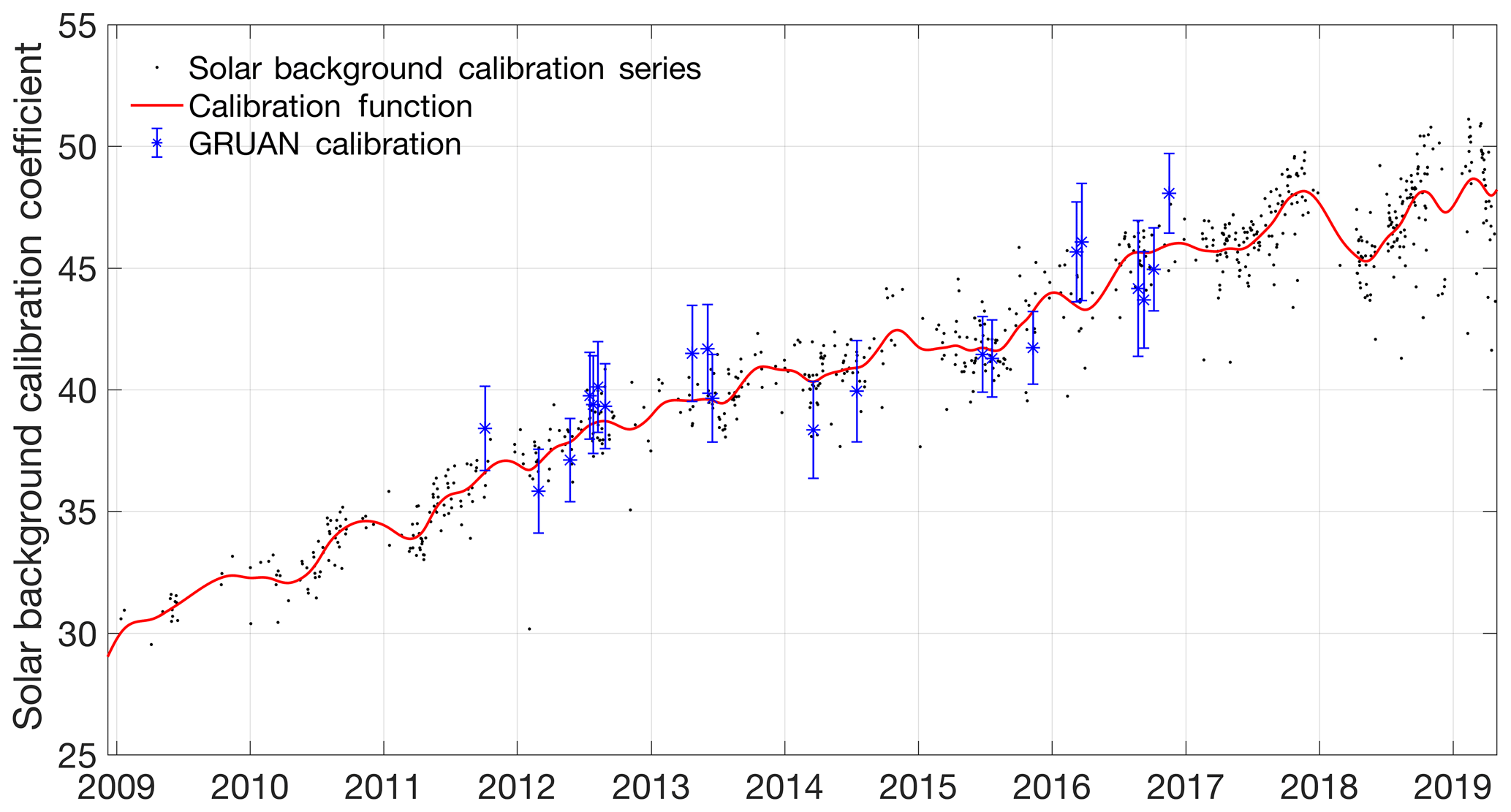
Figure A1 The final normalized calibration time series. Black points are the solar calibration values from January 2009 to August 2019. Blue points are the trajectory calibration values with their uncertainties. The red line is the smoothing spline fit to the solar calibration points.

The calibration coefficient is the constant which converts the relative lidar profile into physical units, such as mixing ratios (g kg⁻¹). When measuring with a constant light source, such as a lamp, the ratio of the signals between the nitrogen and water vapour channels is a measurement of the ratio of each channel's efficiency. Measuring the ratio over time creates the relative calibration time series r_solar(t):

$$\begin{array}{}\text{(A1)}& r_{\mathrm{solar}}\left(t\right)={\displaystyle \frac{N_{\mathrm{H},\mathrm{const}}\left(t\right)}{N_{\mathrm{N},\mathrm{const}}\left(t\right)}},\end{array}$$

where N_X,const(t) is the water vapour or nitrogen signal measured with a constant light source (either a lamp or solar background). This function can then be normalized by an external calibration measurement taken at a time t₀ or by normalizing using an entire time series of measurements such that the new calibration time series becomes

$$\begin{array}{}\text{(A2)}& C\left(t\right)=C_{\mathrm{ext}}\left(t_{\mathrm{0}}\right)r_{\mathrm{solar}}\left(t\right).\end{array}$$

The external calibration (C_ext) at a time t₀ can be chosen at any point in the time series or be an average of several points. The solar background signal for both the nitrogen and water vapour channels can be calculated by taking the average value of the background signal above 50 km. At these altitudes in a raw 1 min profile, the signal is completely due to background solar radiation and not photons emitted by the laser. Therefore, during the daytime, all photons should be solar photons or tube background. One must be careful to consider both the diurnal and seasonal solar cycles when using this technique; therefore, it is important to use the same solar zenith angle each day at the highest-possible angle. The highest solar zenith angle on the winter solstice is 20^∘. Therefore, the calibration is conducted each cloudless morning when the sun is at a solar zenith angle of 20^∘. The ratio of the nitrogen solar background and the water vapour solar background was then used to calculate the r_solar function. We do not correct the solar background time series for differential transmission between the nitrogen and water vapour channels. A sensitivity study using over 3 years of RALMO data was used to assess the value of Δα, where $\mathrm{\Delta }\mathit{\alpha }=(\mathrm{1}-{\mathit{\tau }}_{{\mathrm{N}}_{\mathrm{2}}})/(\mathrm{1}-{\mathit{\tau }}_{{\mathrm{H}}_{\mathrm{2}}\mathrm{O}}$). The study found that the overall impact of the differential transmission correction amounts to a maximum of 5 %, with an average of 2 %. These findings are in agreement with what was found in the study by Whiteman et al. (1992). However, the GRUAN radiosonde calibrations were corrected for differential aerosol transmission (Hicks-Jalali et al., 2018), and the relative calibration time series is scaled by the GRUAN radiosonde external calibration. Scaling the calibration time series with the GRUAN radiosonde calibration creates a continuous calibration time series from 2008 until the end of 2018 (Fig. A1 in Appendix).

The black points in Fig. A1 are the solar background calibration time series. The background values clearly exhibit a linear component, which would indicate that the nitrogen and water vapour photomultipliers are differentially ageing (assuming that the ageing is linear). However, there is also a more complicated behaviour embedded in the time series, particularly towards the end of 2017 and 2018, which would make it inappropriate to simply fit a linear function to the time series. Therefore, we chose to fit a smoothing spline to the time series, which is represented by the red line in Fig. A1. The blue points show the calibration values from Hicks-Jalali et al. (2019) with their respective uncertainties. The abrupt dip in calibration values after 2018 may be due to the installation of a new laser at that time, but the source has not yet been determined.

The uncertainty in the calibration function was estimated using the standard deviation of the de-trended background time series. The percentage of uncertainty is the standard deviation divided by the mean calibration value. It agrees with the average uncertainty of 5 % from the GRUAN calibrations in Hicks-Jalali et al. (2019). While this method did not decrease the uncertainty of the calibration, it allowed the use of a continuous and consistent calibration constant for the entire water vapour time series.