Modelling of the public health costs of fine particulate matter and results for Finland in 2015

We have developed an integrated assessment tool that can be used for evaluating the public health costs caused by the concentrations of fine particulate matter (PM_2.5) in ambient air. The model can be used to assess the impacts of various alternative air quality abatement measures, policies and strategies. The model has been applied to evaluate the costs of the domestic emissions that influence the concentrations of PM_2.5 in Finland in 2015. The model includes the impacts on human health; however, it does not address the impacts on climate change or the state of the environment. First, the national Finnish emissions were evaluated using the Finnish Regional Emission Scenarios (FRESs) model on a resolution of 250×250 m² for the whole of Finland. Second, the atmospheric dispersion was analysed by using the chemical transport model, namely the System for Integrated modeLling of Atmospheric coMposition (SILAM) model, and the source receptor matrices contained in the FRES model. Third, the health impacts were assessed by combining the spatially resolved concentration and population data sets and by analysing the impacts for various health outcomes. Fourth, the economic impacts of the health outcomes were evaluated. The model can be used to evaluate the costs of the health damages for various emission source categories and for a unit of emissions of PM_2.5. It was found that the economic benefits, in terms of avoided public health costs, were largest for measures that will reduce the emissions of (i) road transport, (ii) non-road vehicles and machinery, and (iii) residential wood combustion. The reduction in the precursor emissions of PM_2.5 resulted in clearly lower benefits when compared with directly reducing the emissions of PM_2.5. We have also designed a user-friendly, web-based assessment tool that is open access.

1 Introduction

Air pollution related to particulate matter (PM) can result in a wide variety of impacts. Prominent examples of these include the enhancement or mitigation of climate change, adverse impacts on the health of the population and various consequences for the environment (e.g. influence on biodiversity, acidification and eutrophication). Air pollution may also cause the corrosion of materials and degradation of buildings and cultural heritage (e.g. Al-Thani et al., 2018). Methods to analyse and value such economic benefits have been presented, for example, by Navrud and Ready (2002, 2007) and Watt et al. (2009).

This study focuses on the impacts of air pollution on public health. The projected economic growth, urbanisation and the increased fraction of the senior population will increase the effects on public health in some regions in the future (e.g. OECD, 2016).

Emission standards and other control policies, in many cases, only address the amounts of emissions. Such policies will not be optimal for the mitigation of the impacts of poor air quality as the same amount of emissions from different sources may have totally different damage costs (e.g. Muller and Mendehlson, 2009; Carson and LaRiviere, 2018). Economists have therefore suggested market-based approaches, such as emission taxes (e.g. Baumol and Oates, 1988) or tradable permits. As the marginal damages (defined as the additional damage caused by an additional unit of emission) and the properties of the emission sources, such as emission heights, differ across regions (Nahlik et al., 2016), environmental policies should reflect these differences. It is therefore worthwhile to evaluate the relative costs of potential emission reductions from different emission source categories located in different regions.

There is a fairly extensive amount of scientific literature regarding the cost evaluations of air pollution on public health, including especially the effects of the PM_2.5 concentrations. Muller and Mendehlson (2009), Holland et al. (2015) and Heo et al. (2016) have evaluated the unit costs of the emissions at various stack heights on a fairly fine spatial resolution in the USA at a county level. Buoconore et al. (2014), Levy et al. (2009) and Fann et al. (2009) have conducted similar studies on a coarser resolution in the USA. Moreover, Nahlik et al. (2016) estimated the county-specific unit damage costs for PM (especially PM_2.5), in addition to SO_x, NO_x and VOCs, at major airports in the USA. Trejo-González et al. (2019) analysed economic costs associated with exposure to PM_2.5 in 2013 and 2015 in Mexican cities assuming two mitigation scenarios.

In Europe, Bickel and Friedrich (2005) have developed a thorough methodology for the impact pathway approach called the ExternE methodology. The ExternE methodology provides a framework for presenting numerous and various impacts as monetary values. In particular, Bickel and Friedrich (2005) evaluated monetised health impacts that are differentiated according to height of release and urban versus non-urban areas. They also developed an assessment tool called EcoSenseLE (Light Edition) to easily provide estimations of impacts on human health and of environmental damages caused by air pollution in Europe (http://ecoweb.ier.uni-stuttgart.de/EcoSenseLE/current/index.php, last access: 27 July 2020). More recently, Holland (2014) and Brandt et al. (2010) evaluated unit costs at country level. DEFRA (2015) and Walton et al. (2015) conducted similar studies regionally in Europe.

In Asia, and more specifically in China, Qi et al. (2018) investigated the losses in and the consequences for the economy by ambient PM_2.5. The study by OECD (2016) pointed out that impacts due to PM_2.5 concentrations commonly contribute to more than 90 % of the total health costs of air pollution. Clearly, the exact proportion of these effects depends substantially on the domain and the year of evaluation. Emissions of the most important PM_2.5 precursors, such as NO_x, SO₂ and NH₃, have also been included in some studies (e.g. Walton et al., 2015). The direct health costs of NO₂ and O₃ may also be substantial in some cases.

With respect to unit cost modelling, most studies have used the so-called impact pathway approach. This approach combines air quality modelling with population data, epidemiological evidence and economic modelling (Im et al., 2018). It is a sequential approach in which one assumes a change in emissions, models the corresponding changes in air quality, uses epidemiological evidence to calculate the health response and, finally, applies economic evidence. For instance, Trejo-González et al. (2019) concluded in their study that a reduction in the annual PM_2.5 average to less than 10 µg m⁻³ in 2015 would have decreased mortality by 14 666 (avoidable deaths), with estimated costs of USD 64 164 million, in Mexican cities.

Some previous studies have used chemical transport models on regional or continental scales (e.g. Fann et al., 2009; Buonore et al., 2014; Brandt et al., 2010; Im et al., 2018). Another approach is to use simplified decision support modelling systems that use pre-computed atmospheric dispersion statistics or source dispersion matrices (e.g. Muller and Mendehlson, 2009; Holland, 2014; Holland et al., 2015; Bickel et al., 2003). One example of these approaches was presented by Heo et al. (2016); they attempted to generalise the results of chemical transport models using statistical methods. As this approach substantially reduces the computational effort, one can evaluate a much larger number of various emission reduction scenarios. Heo et al. (2016) computed the resulting changes in air quality for a 1 t reduction in emissions for 11 different emission sources in the USA.

In the next stage of the evaluation, one will evaluate the health impacts caused by the changes in the concentrations. Some of the studies have included only the increased risk of early mortality (e.g. Heo et al., 2016; Buonocore et al., 2014; Levy et al., 2009), due to the fact that mortality costs commonly dominate the total unit costs. In these studies, PM_2.5-induced mortality has been modelled with a linear response function model in which an increase in the concentration levels is linearly translated into either a loss of human lives or years of life lost (YOLL). For example, 144 289 and 150 771 potential YOLLs due to exposure to PM_2.5 were estimated for 2013 and 2015, respectively, in Mexican cities (Trejo-González et al., 2019).

The response functions have been estimated in epidemiological studies, such as Pope et al. (2002), or based on a combination of other studies related to long-term exposure to PM_2.5 and PM₁₀, such as Trejo-González et al. (2019). However, most studies have also included other end points, most commonly the morbidity costs (Muller and Menhdelson, 2009; Holland et al., 2015; Fann et al. 2009; Walton et al. 2015; DEFRA, 2015; EEA, 2014). Some studies (Muller and Mendehlson, 2009; Walton et al. 2015) have also included the loss of agricultural yields; however, these result in a minor effect on the unit costs. In a more recent study conducted by Trejo-González et al. (2019), the lost productivity was also calculated for 2013 and 2015 in Mexican cities for different age groups (15 years and older, 30 years and older, and 25 to 74 years). In China, Qi et al. (2018) estimated that the total national loss due to exposure to PM_2.5 was Chinese Yuan 79.2 billion.

As the increased risk of early mortality commonly dominates the unit cost estimates, the assumptions behind its computation explain a large fraction of the variation in various damage cost estimates. The health response functions contain a risk ratio or relative risk (RR) for an increase in concentration of 10 µg m⁻³ that describes the change in the relative risk level. RR is generally defined as the ratio of the probability of an outcome in an exposed group to the probability of an outcome in an unexposed group. Moreover, RR is different from one region to another, depending on ambient PM_2.5 composition and the variation in the peoples' sensitivity (Qi et., 2018). A low value was applied by Bicket et al. (2003), namely RR=1.024, whereas Pope et al. (2002) estimated a much higher value, namely RR=1.077. The latter estimate has been widely used in unit cost studies (Muller and Mendehlson, 2009; Holland et al., 2016; EEA, 2014). Qi et al. (2018) also applied a low RR for lung cancer related to PM_2.5 in China, and it was equal to 1.03. The same value was used by Cao et al. (2011) and Loomis et al. (2014). The American Cancer Society published an estimate of 1.075 that was used in Heo et al. (2016). A more conservative estimate of 1.06 has been reported in some studies, such as DEFRA (2015) and Raza et al. (2018), apart from Woodcock et al. (2009, 2013 and 2014) and Dhondt et al. (2013). The Harvard Six Cities study (Laden et al., 2006) resulted in an even more substantial mortality, i.e. RR=1.12. This value has also been used widely (Fann et al., 2009; Levy et al., 2009). Raza et al. (2018) presented an even higher RR for PM_2.5 (RR=1.17) in their paper, which was originally reported in another study regarding air pollution and mortality in Los Angeles (Jerrett et al., 2005)

The next step in the analysis chain is to convert the health impacts into monetary values. With respect to mortality, there are two main approaches to the monetary valuation, namely either (i) counting the expected value of life years lost and multiplying that with the value of a life year (VOLY), or (ii) counting the expected value of early mortality and multiplying that with the value of life (VSL). However, both the values of VOLYs and those of VSLs and the final cost results obtained using these two approaches can vary substantially. Regarding the VSL, a fairly low estimated value in Muller and Mendehlson (2009) was USD 2 million, with an age-adjusted value of USD 1.2 million, whereas Heo et al. (2016) evaluated VSL to be USD 8.6 million. VSL was equal to USD 1.629 million and USD 1.643 million in 2013 and 2015, respectively, in the Mexican cities of the national urban system (Trejo-González et al., 2019). EU-based studies have commonly indicated a higher public health cost value using the VSL method, compared with those obtained using VOLY; e.g. the study by EEA (2014) found that the VSL-based values were approximately 2.5 times higher than the VOLY-based values.

Taking into account the concentrations nowadays and during the past decade, particulate matter can be considered, in most locations, to be more harmful than gaseous pollutants; e.g. this has been found to be the case for the Nordic countries by Lehtomäki et al. (2018) and Kukkonen et al. (2018). WHO (2013a) has shown a strong association between the concentrations of coarse and ultrafine particles and harmful effects. In the present study, we have addressed the health impacts of fine particulate matter, including its precursor emissions; however, we have elected not to consider the health effects of NO₂ concentrations. WHO has stated that the effects of NO₂ are partly overlapping with those of PM_2.5 in epidemiological studies (WHO, 2013a–b). The main reason for not addressing NO₂ health impacts in this study was the major uncertainties concerning concentration–response functions. A majority of epidemiological studies have focused on PM_2.5, or alternatively on PM₁₀, and including PM_2.5 as a subfraction, and therefore the most established concentration–response functions have been developed for these size fractions.

The overarching aim of this study is to develop an integrated assessment tool to evaluate the public health costs caused by the ambient air concentrations of fine particulate matter (PM_2.5). The objectives of this study are (i) to present an impact pathway model to evaluate the public health costs due to the concentrations of PM_2.5, (ii) to present selected example results regarding the various stages of this assessment for domestic pollution sources in Finland in 2015 and (iii) to present both an easy-to-use summary tabulation and a web-based computation system for the public health costs for various emission categories. The final model framework includes emission and dispersion modelling, health impact assessment and economic evaluation. The model and results regarding the costs of the emissions from various source categories can be used to assess the economic public health impacts of national and urban scale air quality strategies and those of various potential emission mitigation measures. The model framework could be also adapted for similar economic cost analyses in other countries or geographical domains in future.

2 Methods

This study adopts the impact pathway approach to combine the various modelling stages.

2.1 Inventory of the domestic emissions

The anthropogenic emissions in Finland in 2015 were computed using the Finnish Regional Emission Scenarios (FRESs) model. For a detailed description of the FRES model, the reader is referred to Karvosenoja (2008), Karvosenoja et al. (2011 and 2020) and Savolahti et al. (2016 and 2019). The modelling included the anthropogenic emissions of the compounds PM₁₀, PM_2.5, PM₁, BC (black carbon), OC (organic carbon), mineral dust, SO₂, NO_x, NH₃, NMVOC and CO. The emissions were computed on a grid of 250 m×250 m for the whole of Finland for various area sources. In addition, the modelling included 424 industrial point sources. For the latter, coordinates and stack heights were used that were specific to each installation (Karvosenoja et al., 2011).

The emission scenarios included the most significant pollutants for each source category. These included the following primary emissions: PM_2.5, NO_x and SO₂ for industrial installations and power plants; PM_2.5 and NO_x for vehicular traffic and machineries; PM_2.5 for residential wood combustion; and NH₃ for agriculture. First, we computed a baseline emission scenario for a selected recent year, namely 2015. Second, the emissions from each of the considered emission sectors and considered pollutants were reduced by a constant moderate percentage, selected to be 10 %, and compared with the baseline scenario.

The health damage caused by the population exposure is substantially dependent on the spatial correlation of the distributions of the population and the emission sources (e.g. Soares et al., 2014). Such a correlation can be especially high for vehicular traffic and residential wood combustion. These two emission source categories were therefore separately analysed for two classes, viz. emissions in urban and non-urban areas. In this study, urban areas were defined according to the following two criteria: (i) these had to include grid cells (250 m×250 m) that contained at least 200 residents; (ii) buildings could not be further from each other than 200 m.

For point sources, we have also treated the PM_2.5 emissions separately, depending on the location of the facility. This was done as the population density in the vicinity of various locations varied substantially. We have therefore separately evaluated the unit costs for (i) the Helsinki area, (ii) the municipalities of more than 50 000 inhabitants and (iii) the other areas.

2.2 Atmospheric dispersion modelling

We have evaluated the atmospheric dispersion using the following two models: (i) the chemical transport model, namely the System for Integrated modeLling of Atmospheric coMposition (SILAM) model (e.g. Sofiev et al., 2006, 2015) and (ii) the source receptor matrices contained in the FRES model (Karvosenoja et al., 2011). The SILAM model can be used for regional-, continental- and global-scale evaluations (Sofiev et al., 2018; Lehtomäki et al., 2018; Brasseur et al., 2019), whereas the FRES model is applicable on local and regional scales.

We have used two models, as both their applicability and results are complementary. The model computations using the SILAM model also include the long-range transported contributions from the rest of Europe, whereas the FRES computations address only the dispersion of the domestic emissions. Another advantage of the SILAM model computations is that the formation of secondary PM_2.5 is taken into account, whereas these are not included in the FRES model computations. On the other hand, the FRES computations are substantially less resource-consuming, and we therefore could execute the model on a very fine spatial resolution, namely 250×250 m². In this study, we used the SILAM computations on a resolution of 5×5 km² over the Finnish domain.

The impacts of the various domestic emission reduction scenarios were evaluated by numerically changing the Finnish emissions of a selected source category, whereas the emissions from the other domestic source categories were kept the same. In the SILAM computations, the emissions from the rest of Europe were also assumed to be the same for all the emission scenarios. In this way, one can evaluate the impact of one selected national source category on the concentrations of PM_2.5.

First, we computed atmospheric dispersion for the baseline emission scenario in 2015, using actual meteorological data for that year. Second, the atmospheric dispersion was computed for the reduced-emission scenarios described above. Finally, the differences in these two computations were computed, and the results were converted to correspond to a reduction in a unit mass of emissions.

2.2.1 Modelling using the SILAM model on the European and national scales

SILAM is a dispersion model from global to mesoscales that has been developed for evaluating atmospheric composition (Sofiev et al., 2015). The model is also used for policy guidance in case of emergencies and for solving inverse dispersion problems. The model includes dispersion and transport treatments, using both Eulerian and Lagrangian approaches. The model contains eight chemical and physical transformation modules, viz. basic acid chemistry and secondary aerosol formation, ozone formation and transformation in the troposphere and the stratosphere, radioactive decay, aerosol dynamics, and transformation of pollen (Sofiev et al., 2010; Kouznetsov and Sofiev, 2012; Sofiev, 2017). The model components and set-up used in the current study have been described and evaluated by Prank et al. (2016), Kollanus et al. (2016), Petersen et al. (2019) and Karl et al. (2019). The model also includes modules for 3D and 4D variational and ensemble Kalman filter (EnKF) data assimilation (Viras and Sofiev, 2012, 2015; Vira et al., 2017).

The computations using the SILAM model included both global- and European-scale transport and the contributions from the domestic (Finnish) emission sources. The modelling for the whole of Finland was carried out on a resolution of 5 km. A detailed description of these computations has been previously presented by Lehtomäki et al. (2018).

The SILAM model computations also included the impacts of the chemical and physical transformations on the formation of secondary PM_2.5. These reactions include, especially, the impacts of the emissions of sulfur, nitrogen and ammonia compounds of both natural and anthropogenic origin on the concentrations of PM_2.5. In the model calculations, the full spectra of emitted compounds were included, separately taking into account the temporal variations for each individual sector. The modelling also allowed us to simultaneously treat the sectoral specifications of the point and area sources. This enabled us to independently estimate the contributions of the emission reductions on PM_2.5 concentrations that originated from power plants, industry, traffic and agricultural ammonia.

2.2.2 Modelling using the FRES model on the national scale

The FRES model was applied for the evaluation of the impacts of primary domestic emissions. These computations had a spatial resolution of 250×250 m² over the whole of Finland. The source receptor matrices that were used in this model were based on the computations using the dispersion model called the Urban Dispersion Modelling system by the Finnish Meteorological Institute (UDM–FMI; e.g. Karppinen et al., 2000a).

The UDM–FMI model is based on Gaussian plume equations for multiple sources, including stationary point, area and volume sources. The modelling system including the UDM–FMI model has been previously extensively evaluated against urban measurement data for gaseous pollutants (e.g. Karppinen et al., 2000b; Kousa et al., 2001) and for PM_2.5 (e.g. Kauhaniemi et al., 2008; Kukkonen et al., 2018, 2020).

The source receptor matrices were based on separate computations over 10 climatic subzones in Finland, assuming two different emission heights. Such computations were necessary as the dispersion processes are strongly dependent on the climatic variation of the relevant meteorological conditions. The computations were performed on an hourly basis for a period of 5 or 6 years for each of the 10 climatic zones, depending on the availability of the relevant meteorological data. In the final computations using the FRES model, monthly average source receptor matrices were used.

2.3 Health impact assessment

In this assessment, we have not explicitly allowed for the health effects caused by the NO₂ concentrations. One reason for this choice is that, in evaluating the health impacts of PM_2.5, we have already allowed for the secondary PM_2.5 concentrations that have resulted from the NO and NO₂ precursor emissions. Including the health impacts in the case of the NO₂ concentrations would therefore result in double counting. Another reason for not explicitly including the health impacts of NO₂ exposure is that the concentration–response function for NO₂ has an effective range for annual average concentrations exceeding 20 µg m⁻³; the concentrations of NO₂ are commonly lower than this threshold value in the present study.

We have combined the modelled annually averaged concentrations of PM_2.5 with the population count data provided by Statistics Finland in 2015. These data sets were combined in a 250×250 m² grid for 5-year age categories. The health effects of PM_2.5 were assumed to be linear in the concentration range observed in Finland. It was therefore possible to use annual concentration data for the computations of the health impacts regarding both short- and long-term exposures.

We have computed the health impacts for each grid cell (i) within the domain (i.e. the whole of Finland). The exposure of the population to the concentrations of PM_2.5 in a grid cell is as follows:

$${\displaystyle }{\displaystyle }{\text{PE}}_i=P_i\times C_i,$$

where P_i and C_i are the population and concentration in the grid cell i, respectively. For each health outcome, the effect of the PM_2.5 exposure was estimated by calculating the relative excess risk (RER) as follows:

$${\displaystyle }{\displaystyle }\text{RER}=(\text{RR}-\mathrm{1})\times \mathrm{0.1},$$

where RR is the risk ratio for PM_2.5 for the considered health outcome.

The computation takes into account that risk ratios for PM_2.5 are usually presented in terms of a 10 µg m⁻³ increase in concentration. However, for some health outcomes, reliable risk ratios have only been established for PM₁₀. In such cases, the RER of PM₁₀ multiplied by 1.54 was used, as recommended by WHO (2013b). The underlying assumptions, when deriving this numerical value, were that the PM_2.5 concentration constitutes 65 % of the PM₁₀ concentration, and the health effects of PM₁₀ can be explained by PM_2.5.

The number of cases of a considered health outcome in each grid cell was calculated as follows:

$${\displaystyle }{\displaystyle }{N}_i={\text{PE}}_i\times \text{RER}\times \text{BR},$$

where BR is the background risk of a considered health outcome. The total impact of PM_2.5 exposure on an outcome was calculated by summing the numbers of cases over all the grid cells. We computed the total number of years of life lost due to the PM_2.5 exposure by (i) multiplying the evaluated deaths with life expectancy into 1-year age categories and (ii) subsequently summing the lost life years over all the age categories.

The exposure to fine particulate matter has been reported to be associated with a substantial number of health outcomes in epidemiological studies (Qi et al., 2018; Raza et al., 2018; Im et al., 2018); however, reliable estimates of the concentration–response functions have been derived only for a limited number of outcomes. In this study, the functions recommended within the Health Risks of Air Pollution in Europe (HRAPIE) project were used (WHO, 2013b). These functions have been considered sufficient to enable the quantification of both the effects of the long-term PM_2.5 exposures on mortality and the short-term exposures on cardiovascular and respiratory hospital admissions (Im et al., 2018).

We did not use any threshold for the PM_2.5 effects, as even relatively low levels of PM_2.5 have been associated with health effects (e.g. Halonen et al., 2009) and even mortality (WHO, 2013a; Raza et al., 2018). It is also biologically plausible that a threshold for the effects does not exist due to the nature of the proposed physiological mechanisms of the effects, such as systemic inflammation (e.g. Lanki et al., 2015). However, in some recent global impact assessments, a lower cut-off concentration has been used (Gakidou et al., 2017).

We have also made the simplification that the health effects of PM_2.5 were the same per mass unit for all emission source categories. The chemical composition of PM_2.5, and consequently the emission source, has been found to modify the health effects. For example, it has been suggested, based on toxicological studies, that secondary PM_2.5 may be less harmful that primary PM_2.5. However, the current consensus is that the PM_2.5 sources cannot be ranked with respect to harmfulness, as the evidence is not sufficient for doing so (WHO, 2013a; US EPA, 2009).

Many of the health effects of PM_2.5 are lagged in time, whereas in the model all effects are treated as immediate ones. On one hand, the effect of the lag time is irrelevant if the considered timescale is very long. This is commonly the case for policy measures to curb PM_2.5 emissions; these are characteristically designed to be long-term solutions. On the other hand, the uncertainty of the cost estimates will increase over decades as the population size and location, age structure, background risks and willingness to pay for better health will inevitably change.

The considered health outcomes have been presented in Table 1. These outcomes are mainly long-term effects. There is also sufficient evidence for the effects of short-term exposures on mortality, but, as the short-term effects can be considered to be included in the estimates of the long-term effects, they were not explicitly included in the model. Regarding the restricted activity days, we did not include the days spent in a hospital (based on calculations on hospital admissions) or at home (calculations on lost work days) to avoid double counting.

Table 1 The considered health outcomes, age groups, types of exposure, risk ratios per concentration difference, their confidence intervals and annual background risks.

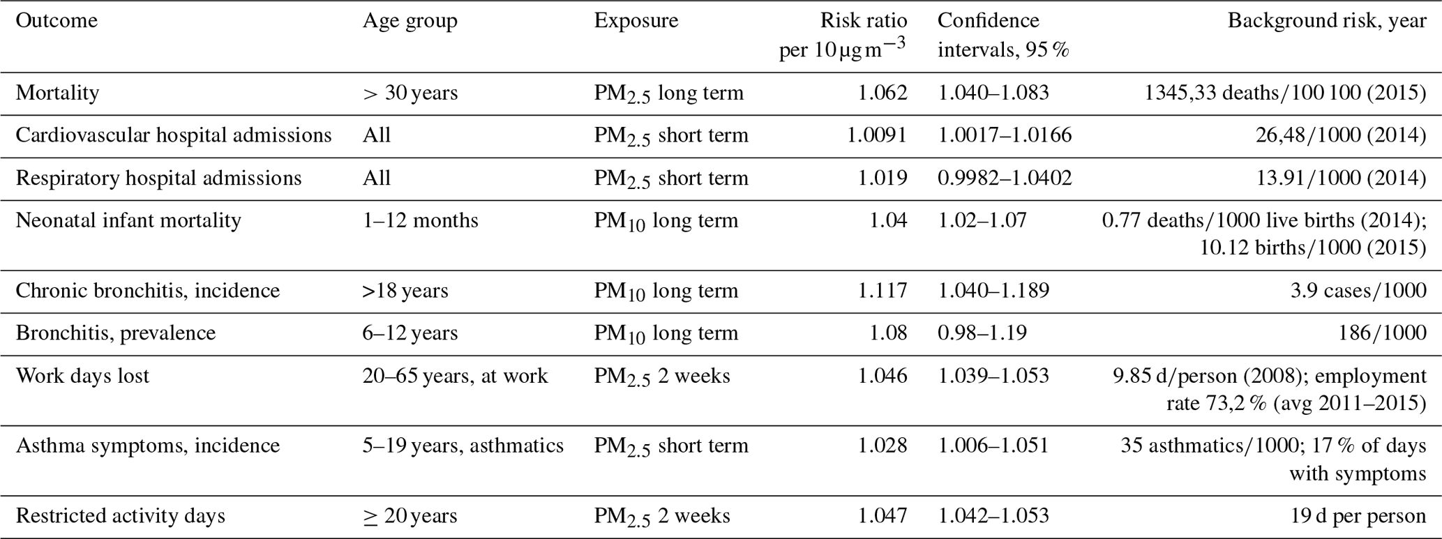
The evidence for the concentration–response functions is stronger for mortality and hospital admissions, compared with the other health effects listed in Table 1. The concentration–response functions were nevertheless also provided for other health effects in the HRAPIE project. The causal association for these effects can be considered to be probable; however, the magnitude of these effects cannot be precisely determined. We have included such effects in the model to avoid an underestimation of the total health impacts. For the mortality, a risk ratio of 1.062 was used, which can be considered to be a state-of-the art value (e.g. Walton et al., 2015).

Some impacts of PM_2.5 have not been calculated for the total Finnish population but for a specific age group. This selection was caused by the limitations of the epidemiological studies that provided the concentration–response functions. The HRAPIE project recommends computing the impact of PM_2.5 exposure on the restrictions of physical functioning without age limitations, although the original epidemiological study that provided the concentration–response function was conducted on a working-age population (Ostro, 1987). As a compromise, we have computed the impact in both working-age and elderly populations but not for children, where the effect was considered to be too uncertain.

Concentration–response functions correspond to the relative effects of PM_2.5. In addition, information on the background risk is therefore needed for each outcome to calculate the actual impact. In this study, the background risk of mortality was obtained from Statistics Finland and the information on hospital admissions from Eurostat. Other estimates of the background risk are based on previous EU-wide impact assessments (Hurley, 2005; Holland, 2014).

2.4 Assessment of the economic impacts

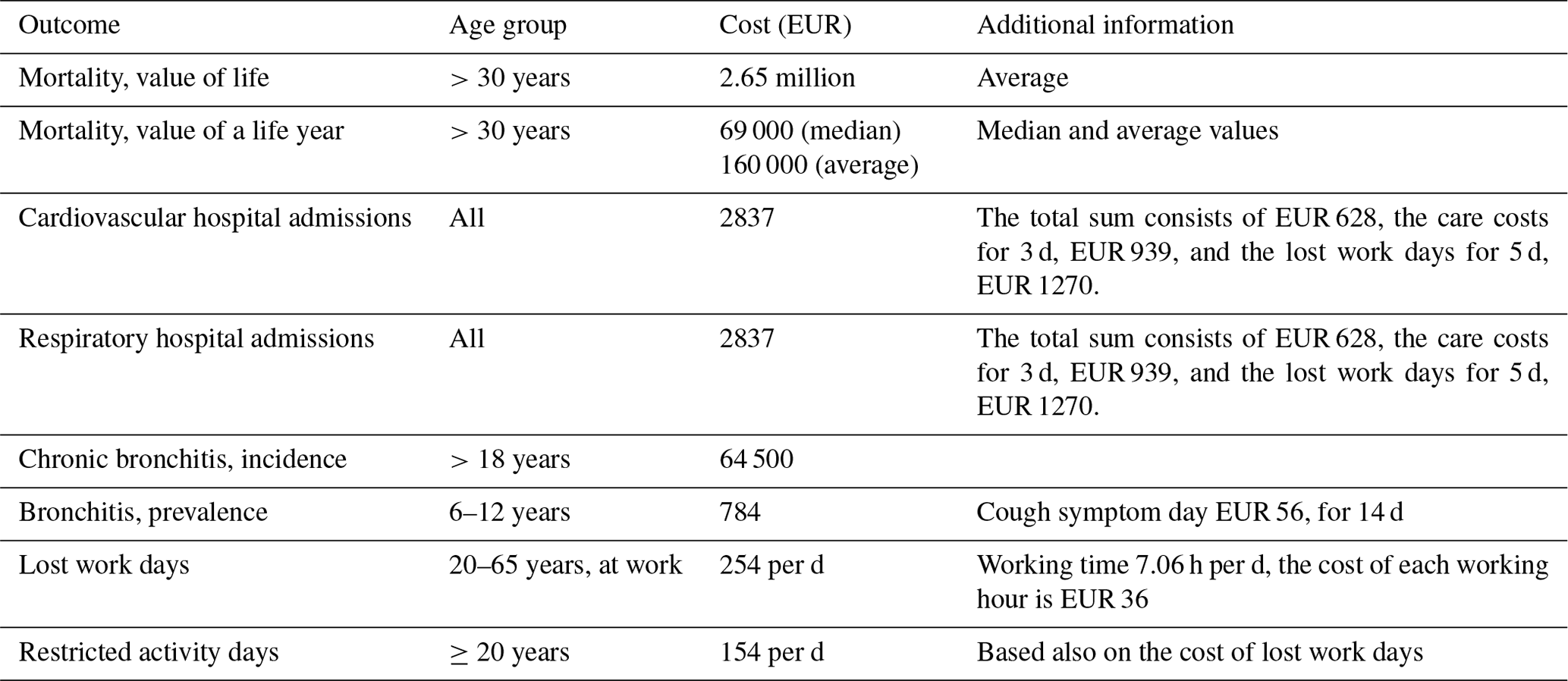
The economic cost values applied in the computations are presented in Table 2. The costs have been mainly selected according to the previous EU-wide impact assessments by Hurley et al. (2005) and Holland (2014). This also facilitates numerical comparisons with those studies. The mortality effects have the largest impact on the total costs; the evaluation of the unit cost for mortality was therefore the most crucial parameter for the final results.

Table 2 The unit costs (in EUR) of the health outcomes that were included in the model. All values are mainly based on the willingness-to-pay approach.

Alternatively, a country-specific VSL (and a derived VOLY from this VSL) for Finland could be applied in this analysis. Such a value could be based on a value transfer (Navrud and Ready, 2007) from the most recent global meta-analysis of the stated preference studies of VSL (Lindhjem et al., 2011). However, this would preclude the direct comparison of results with similar impact pathway models, such as Holland et al. (2005).

The monetised estimates in the computations of the economic impacts in this study were based both on the average value of a life year (VOLY) and the value of statistical life (VSL). The choice between the VOLY and VSL approaches is also an ethical question. In order to obtain more objective results, less dependent on any ethical evaluations, we elected to use both measures. In the VSL approach, the increase in relative risk is uniformly applied to all the age groups, whereas in the VOLY approach the relative risk is unequally distributed within the various age groups. However, some studies have adjusted for this factor (e.g. Muller and Mendehlson, 2009). In other words, the selection of VOLY or VSL includes whether one should assign the same economic value to all adults, independent of their age. Assuming a constant VOLY also implies that people value a life year in the same way, independent of their age.

The VOLY-based approach has been commonly used as a measure to assess a decrease in the mortality risk (Im et al., 2018), whereas the VSL-based approach is in line with the Environmental Protection Agency's standard procedure and recommendations (Wolfe et al., 2019). VSL has been used in many studies in the USA (i.e. Nahlik et al., 2016; Trejo-González et al., 2019; Wolfe et al., 2019), while mainly VOLY has been used in studies within the EU (Im et al., 2018). The VSL-based approach results in higher economic cost values (e.g. EEA, 2014).

We have used both the average and median values of VOLY in this study. However, the average value may correspond better to the willingness to reduce risks on a population level.

The unit cost of chronic bronchitis used in this study (EUR 200 000) was substantially lower than the corresponding value used in the previous EU-wide assessment by Hurley et al. (2005). The cost estimate used here is based on the meta-analysis conducted in the Health and Environment Integrated Methodology and Toolbox for Scenario Assessment (HEIMTSA) project; this new value has also been used in the most recent EU-wide assessment (Holland, 2014).

The cost of a hospital admission is partly based on the willingness-to-pay (WTP) approach, as estimated by Ready et al. (2004). The WTP estimate takes into account 3 d in hospital care (because of a respiratory disease) and 5 d of bed rest at home. In addition to WTP, direct health care costs (3 d) and lost work days (5 d) contribute to the total cost of a hospital admission. The health care cost estimate used in the calculations corresponds to the mean cost of an acute care admission (<90 d) in primary care in Finland. The original unit cost has been adjusted for 2017 using data from Statistics Finland on the temporal changes in health care costs in Finland.

The estimated cost of a working day in Finland originates from 2012. The value has been adjusted for 2017 using the labour cost index reported by Statistics Finland. The cost of a restricted activity day consists of the cost of lost work days and WTP costs of minor restrictions (symptoms) and more severe restrictions (bed rest at home). The WTP values are based on Ready et al. (2004). For the working-age population, it was assumed that 25 % of the restricted activity days were spent in bed at home, 25 % with symptoms at home and 50 % at work with symptoms. Persons that are eligible for retirement (>65 years; 25 % of the adult population) were assumed to spend 35 % of the restricted activity days in bed and the rest suffering from symptoms.

We adjusted the unit costs for inflation but not for the changes in the income levels, which is in accordance with the practice in the previous EU-wide assessment by Holland (2014). The WTP values were selected according to Ready et al. (2004), in which the results have been reported in GBP in 1998. In this study, these have been converted to EUR using the purchasing power parity index, and to the values in 2017, using the Harmonised Index of Consumer Prices.

3 Results

3.1 Summary of the emissions of PM_2.5 and its main precursors in Finland

The total primary and main precursor emissions (for NO_x, SO₂ and NH₃) of PM_2.5 in Finland in 2015 have been presented in Fig. 1. Regarding the primary emissions of PM_2.5, the most important domestic pollution source categories were residential combustion (10.2 kt a⁻¹) and vehicular traffic and machinery (6.6 kt a⁻¹). The energy production and industrial combustion units and industrial processes were responsible for smaller proportions of the primary emissions of PM_2.5 (2.5 and 1.6 kt a⁻¹, respectively).

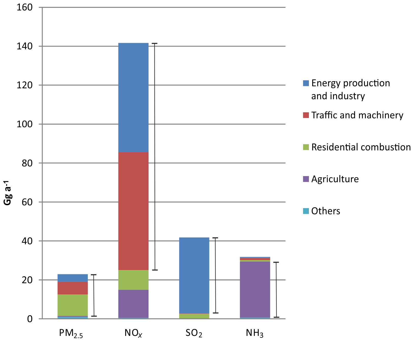
Figure 1 The total amounts of the annual emissions in Finland in 2015 for the pollutants and source categories that were taken into account in this study (Mt yr⁻¹). The NO_x emissions were defined as the sum of NO and NO₂ and presented as the mass of NO₂. The vertical bars show the emission source categories that were included in the simplified web-based assessment tool.

Regarding the emissions of nitrogen oxides, vehicular traffic and machineries and the energy production and industry were the most important source categories. The emissions of sulfur dioxide mostly originated from energy production and industry, and the emissions of ammonia mostly originated from the agricultural sector.

Karvosenoja (2008) has previously evaluated the uncertainties of the national annual average emission estimates of PM_2.5 for residential combustion and vehicular traffic. The estimates of uncertainties included both of those for the use of fuels and for emission factors. The uncertainties were estimated to range from −36 % to +50 % for residential combustion and from −11 % to +13 % for vehicular traffic, within a 95 % confidence interval. The uncertainties of the emissions from point sources were found to be on the same level or lower than those for residential combustion. The uncertainties of the PM_2.5 precursor emissions were on the same level or lower than those for the primary PM_2.5 emissions.

Emissions from shipping have not been included in the above-mentioned inventory. However, shipping emissions on a high resolution were used as input values in the SILAM model computations; this is described in more detail by Lehtomäki et al. (2018). The shipping emissions were provided by the computations using the Ship Traffic Emission Assessment Model (STEAM; e.g. Johansson et al., 2017).

3.2 The modelled changes in spatial concentration distributions caused by the changes in emissions

The atmospheric dispersion, and the changes in concentrations caused by the reductions in emissions, were evaluated for (i) vehicular traffic, (ii) working and off-road machinery, and (iii) small-scale residential combustion. The analyses were made separately for urban and non-urban areas. In addition, in the case of residential wood combustion, we separately assessed the dispersion that originated from (i) fireplaces and sauna stoves and (ii) holiday houses and the boilers of detached houses.

The computations were made partly using the FRES model and partly using the SILAM model. The FRES model was mostly used for evaluating the reductions in concentrations caused by primary emissions (i.e. the emissions of PM_2.5). We used the FRES model for this purpose as the spatial resolution was finer when compared with the SILAM model computations. The SILAM model was used for evaluating the reductions caused by the emissions of pollutants that form secondary particulate matter in the atmosphere; the treatments of the FRES model do not include those processes.

The considered secondary pollutants in the following results include the most substantial ones for each source category; we did not evaluate the impacts of the complete range of secondary pollutants. The secondary pollutants included NO_x, which originated from vehicular traffic and machineries, NH₃, from agriculture, and SO₂ and NO_x, from power plants and industry. In addition, the SILAM model was used for evaluating the effects of the reductions in primary PM_2.5 that originated from power plants and industry; this was done to achieve a better consistency in the predicted results with regards to the two considered secondary pollutants for this source category.

3.2.1 Vehicular traffic, working and off-road machinery and residential wood combustion evaluated using the FRES model

The predicted reductions in the concentrations of PM_2.5 are presented separately for urban and non-urban areas in Fig. 2a–d for vehicular traffic and working and off-road machinery. The computations were conducted using the FRES model on a spatial resolution of 250×250 m².

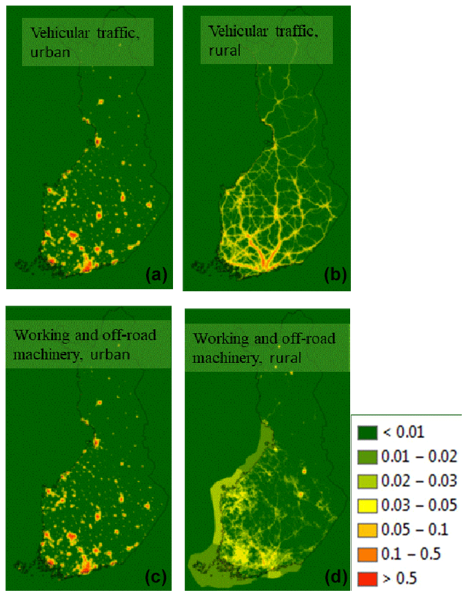
Figure 2 The reductions in concentrations of PM_2.5 (ng m⁻³), caused by a reduction in emissions of PM_2.5 by 1 t. The results are presented for vehicular traffic (a, b) and working and off-road machinery (c, d). For both source categories, the changes in urban and non-urban areas are presented separately, in (a, c) and (b, d), respectively. The spatial resolution is 250×250 m².

As expected, the urban reductions were focused on the largest urban agglomerations, namely cities and towns, for both source categories. The non-urban vehicular reductions were focused on the main road and street network, especially in the most densely populated southern and western parts of the country. The machinery reductions were located within the most industrialised regions, most of which are located in southwestern Finland; these were dispersed across a wider area when compared with the corresponding vehicular traffic reductions.

The predicted reductions in concentrations of PM_2.5 are presented in Fig. 3a–d for three segments of residential wood combustion. The reductions for fireplaces and sauna stoves are presented separately for urban and non-urban areas, whereas both the reductions in holiday homes and in the boilers of detached houses are presented in one panel for the whole country. The computations were conducted using the FRES model on a spatial resolution of 250×250 m².

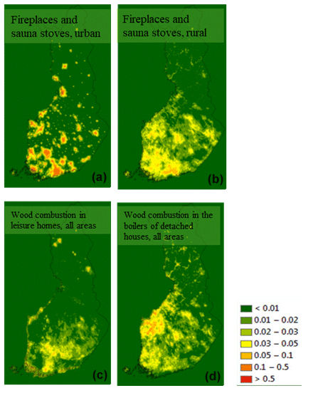
Figure 3 The reductions in concentrations of PM_2.5 (ng m⁻³), caused by a reduction in emissions of PM_2.5 by 1 t that originated from small-scale residential combustion. The changes due to the emissions in fireplaces and sauna stoves are presented in (a, b), and the changes due to the emissions in holiday houses and in the boilers of detached houses are presented in (c, d). For both source categories, the changes in urban and non-urban areas are presented separately, in (a, c) and (b, d), respectively. The spatial resolution is 250×250 m².

As expected, the urban reductions in the emissions for fireplaces and sauna stoves were focused on the largest urban agglomerations. However, the urban reductions in holiday homes and in the boilers of detached houses were much more evenly distributed. The reductions for holiday homes are, as expected, mostly situated in southern central Finland; this area has the most dense network of holiday homes. The reductions from the boilers of detached houses are focused mostly in western Finland; this is caused by the differing cultural habits and preferences regarding housing in different parts of the country.

Kukkonen et al. (2018) recently evaluated the uncertainties of the modelling system containing urban-scale models, namely the Urban Dispersion Modelling system by the Finnish Meteorological Institute (UDM–FMI) and the Contaminants in the Air from a Road by the Finnish Meteorological Institute (CAR–FMI). The UDM–FMI model was used for computing the source receptor matrices within the FRES model. They evaluated the performance of the modelling system extensively against the observations of PM_2.5 concentrations during 16 years at five measurement stations in the Helsinki metropolitan area. The uncertainties of the predicted annual average concentrations of PM_2.5 ranged from −18 % to +15 %.

3.2.2 Evaluation of vehicular traffic, machineries, agriculture and power plants, and industry using the SILAM model

The reductions in PM_2.5 concentrations computed with the SILAM model are presented in Fig. 4a–e. The model grid covered the whole of Finland with a spatial resolution of 5×5 km².

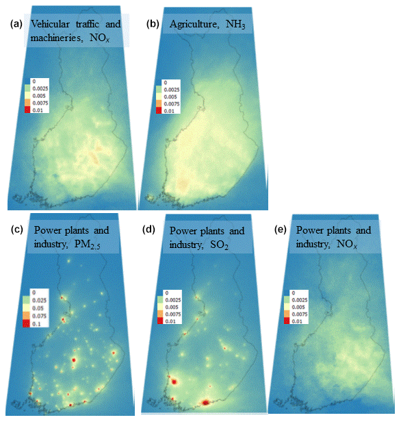
Figure 4 The reductions in concentrations of PM_2.5 (ng m⁻³), caused by a reduction in emissions of 1 t of corresponding pollutants originating from three source categories. The panels present the decrease in concentrations due to reductions in the following emissions: (a) NO_x originating from vehicular traffic and machineries, (b) NH₃ originating from agriculture, (c) PM_2.5 originating from power plants and industry, (d) SO₂ originating from power plants and industry, and (e) NO_x originating from power plants and industry. The spatial resolution is 5×5 km². The scale of reductions is different for (c).

The most prominent PM_2.5 reductions in the close vicinity of the emitting sources were caused by the decrease in primary emissions of PM_2.5 that originated from power plants and industry. A similar result was achieved for the PM_2.5 reductions caused by SO₂ emissions reduction; however, the absolute values of the reduction were an order of magnitude smaller when compared with those caused by the PM_2.5 emission reductions. This was caused partly by the fact that most SO₂ originated from relatively few major power plants and industrial regions and partly by the fairly slow chemical formation of sulfates.

The spatial patterns of the reduced PM_2.5 concentrations were more homogeneously distributed over Finland in the case of lowered emissions of the secondary pollutants NO_x and NH₃. This was caused by the relatively longer timescales of the relevant chemical reactions and by the geographical locations of the main sources of NO_x and NH₃, which are agricultural activities and vehicular traffic networks.

The predictions of the SILAM model have previously been extensively evaluated against monitoring data. For most cases there were fairly good or good agreements, with a slight underestimation of PM concentrations (Prank et al., 2016). Most recently, Lehtomäki et al. (2018) evaluated the accuracy of the SILAM model for predicting the annual average concentrations of PM_2.5. The predicted annual average values were, on average, 5 % lower than the observations at 37 stations in Finland in 2015.

3.3 The health impacts

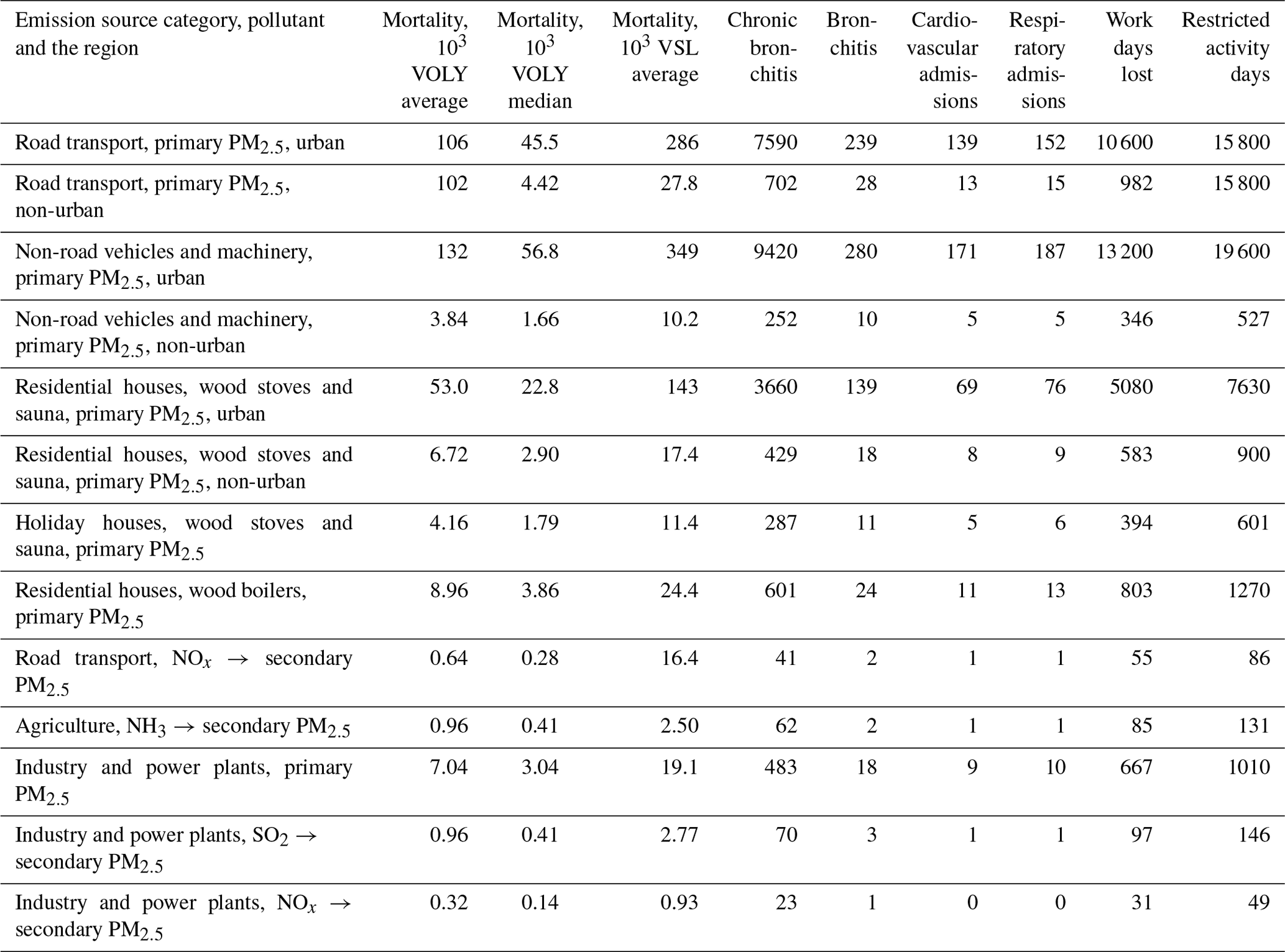
The health impacts were evaluated based on the atmospheric dispersion computations addressed in the previous section. The impacts are presented in Table 3. The units of the values are different for the different columns. For instance, the values in the column “mortality” are the numbers of the cases of premature deaths, and the values in the column “lost life years” are in years. The reported values are incremental health impacts, i.e., the presented impacts correspond to a unit amount (1 kt) of emissions. The values are therefore not the total health impacts within the country.

Table 3 The health impacts caused by an emission of 1 kt of PM_2.5, NO_x, NH₃ or SO₂ in Finland in 2015 for various domestic pollution source categories in various regions. The notation, for example “NO_x → secondary PM_2.5”, refers to secondary fine particulate matter that originated from the emissions of nitrogen oxides.

In general, the impacts were largest in the case of primary PM_2.5 emissions when compared with those for the corresponding secondary pollution. As expected, the impacts in urban areas were also substantially larger than the corresponding impacts in non-urban areas. Regarding the pollution source categories, the most important were non-road vehicles and machinery, road transport in urban areas, and wood stoves and saunas in residential houses.

In addition to the above-mentioned health impacts, the infant mortality and the asthma symptoms were also considered. However, these impacts were negligible when compared with other considered impacts. In the case of infant mortality, the background risk was very low, and for the asthma symptoms, both the prevalence and risk ratio were low. Infant mortality and asthma were therefore excluded from further analysis.

The uncertainty of the health effect values can be estimated based on the adopted concentration–response functions. The majority of the public health costs are related to premature mortality. We therefore address here the average concentration response for the PM_2.5 related to mortality, which has been assumed to be 1.062 (see Table 1) with a linear dependency with respect to the concentration. The 95 % confidence limits of this value range from 1.040 to 1.083. We therefore conclude that the lowest and highest health effect estimates (within the 95 % confidence interval) could be approximated by multiplying by the predicted health effect values by 0.65 (i.e. 4.0 %∕6.2 %) and 1.3 (8.0 %∕6.2 %).

3.4 The economic impacts

We have assessed the economic impacts of the selected potential PM_2.5 emission reductions based on the health impacts addressed in the previous section. These have been computed for a change of 1 t of the annual emissions for the selected pollutants in 2015. The results include only the impacts of the Finnish emissions to the population in Finland; i.e., the health impacts caused by the Finnish emissions in other countries have not been evaluated.

First, the estimated contributions to the total costs were evaluated for the various health outcomes. The detailed results of these computations are presented in Appendix A. The mortality effects were clearly the largest factor affecting the total costs. However, the costs associated with restricted activity days, lost working days and chronic bronchitis were also found to be substantial.

The final results of the economic cost computations are presented in Table 4. The values in Table 4 have been presented for the following three alternative options to compute the economic impact: (i) the average value of life year (VOLY), assumed to be equal to EUR 160 000, (ii) the median value of life year, assumed to be EUR 69 000, and (iii) the average value of statistical life (VSL), assumed to be EUR 2.65 million.

Table 4 Economic benefits obtained from the assumed reductions in emissions in 1000 EUR per tonne of emissions. The results are presented for the various source categories in various domains. The first presented value has been computed based on the average value of life year, and the two values in parenthesis are based on the median value of life year and the average value of statistical life, respectively.

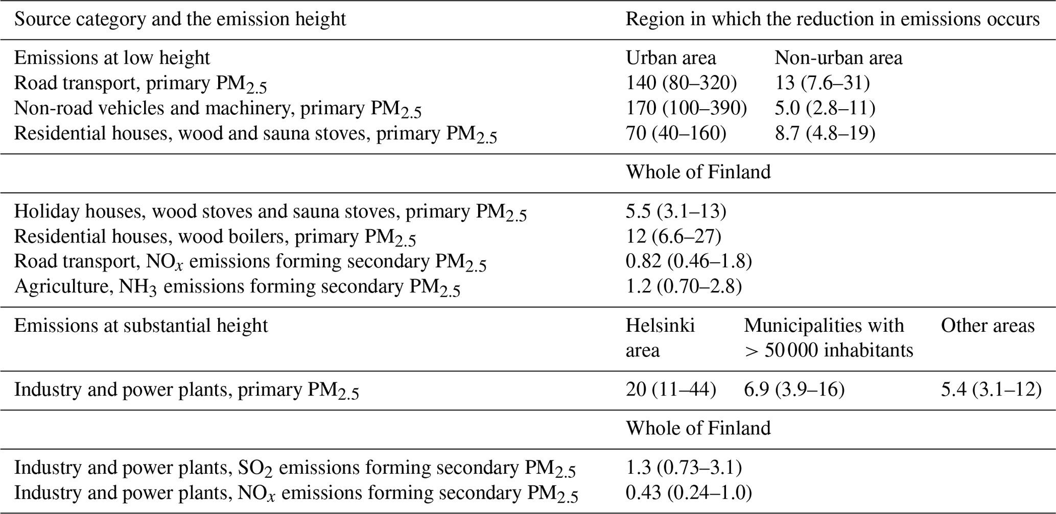
The results have been presented separately for the source categories that have relatively lower and higher emission heights, respectively. The latter category includes the industrial pollution sources and power plants. The results have also been presented in terms of the pollutant, of which the emissions have been assumed to have decreased; these include both primary PM_2.5 and the main precursor substances. For the most significant source categories and substances, the results have also been presented separately for various types of areas, such as the urban and non-urban areas. For the primary PM_2.5 emissions from industry and power plants, the results were presented separately for areas with different population densities; these included the Helsinki area and relatively more and less densely populated municipalities, respectively.

There are substantial variations in the results, depending on the economic computation methods (average or median VOLY or VSL). However, the order of these results is the same for all the results; e.g. the computation using VSL results in the highest economic values. We have therefore illustrated the results computed with one of these methods, i.e. the average of VOLY in Figs. 5a–b and 6a–b. These figures therefore can be used to illustrate the relative economic benefits of the selected emission reduction alternatives.

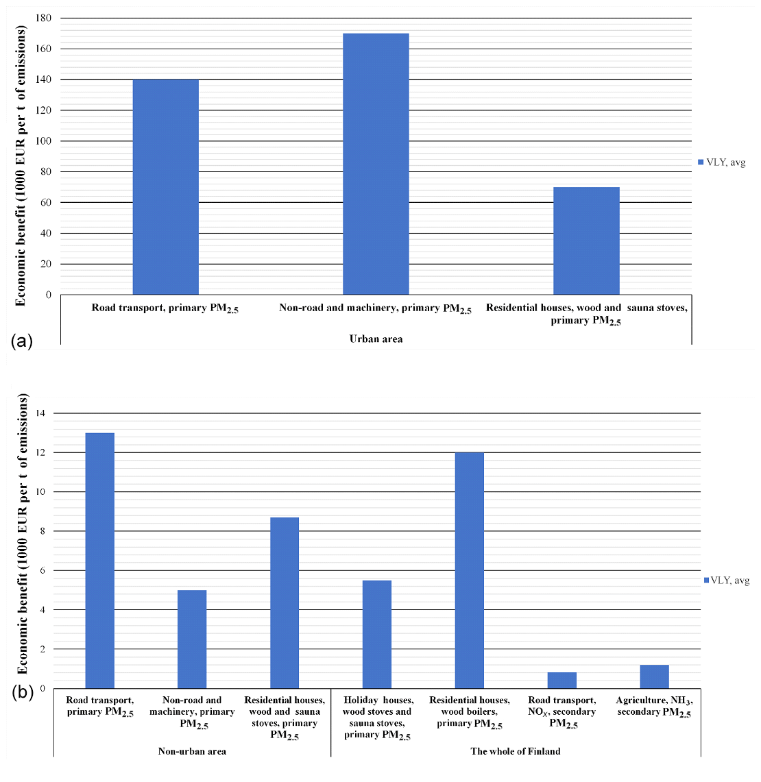
Figure 5 Economic benefits obtained from the assumed reductions in emissions, in 1000 EUR per tonne of emissions, for sources having a low emission height. The results are presented for urban areas (a) and for non-urban areas and for the whole country (b) in the cases of various source categories and pollutants in various domains. All the values correspond to the computations using the average value of life year (VLY).

Figure 6 Economic benefits obtained from the assumed reductions in emissions, in 1000 EUR per tonne of emissions, for sources having a high emission height. These results are presented for industry and power plants. (a) Results for the emission reductions in PM_2.5 for various geographic regions and (b) for the emission reductions in SO₂ and NO_x for the whole of Finland. All the values correspond to the computations using the average value of life year (VLY).

The economic benefits are clearly the largest for the emission reductions for the source categories that have low emission heights (Fig. 5a and b) compared to those with substantial emission heights (Fig. 6a and b). For both kinds of source categories, the reductions, as expected, result in higher public health benefits in the more densely populated regions. For instance, the reductions in the PM_2.5 emissions that originated from vehicular traffic, non-road vehicles and machinery, and residential wood combustion in urban areas result in approximately an order of magnitude higher for economic benefits when compared to the impacts of the corresponding emission reductions in non-urban areas. The results also show that the reduction in the precursor emissions of PM_2.5, such as NO_x, NH₃ and SO₂, was clearly less effective for reducing both the PM_2.5 concentrations and the adverse economic impacts when compared to directly reducing the emissions of PM_2.5.

The uncertainties of the economic evaluations can be estimated based on the differences in the three alternative methods, i.e. those based on the average and median VOLY and the one based on the average VSL. Assuming that the average VOLY would be the base value (denoted here as 1.0), the uncertainty of this estimate would range from 0.57 to 2.2.

3.5 An open-access assessment tool for evaluating the economic impacts

We have also designed and implemented a user-friendly internet-based assessment tool for evaluating the health costs of various assumed emission reduction options. This tool was designed to facilitate an easy use of the model for policy makers, stakeholders and environmental experts. The tool can be accessed via a user-friendly interface on the internet (https://wwwp.ymparisto.fi/IHKU/haittakustannuslaskuri/, last access: last access: 7 August 2020). This calculator is based on the numerical results of this study (such as those presented in Table 4); however, some minor simplifications were made regarding the included emissions. The included emission source categories have been presented by the vertical bars in Fig. 1.

The internet-based tool requires, as an input value, the amount of reduced emissions (t yr⁻¹) for a source category, pollutant and region, which corresponds to a selected abatement measure, bundle of measures or strategy. The tool can then be used to compute, as an output, the annual financial benefits of the measure or strategy (in EUR), and the results are presented both tabulated and graphically. For instance, if the policy maker has an estimate of (i) the emission reduction that could be achieved by a potential abatement measure and (ii) the economic cost of implementing the measure, he or she can use the tool to analyse whether the measure would result in more substantial economic benefits when compared to the costs. Clearly, the tool could also, in such a case, be used for comparing the cost-effectiveness of alternative potential emission reductions.

4 Conclusions

We have presented an integrated assessment tool for evaluating the public health costs of fine particulate matter (PM_2.5) in ambient air. The atmospheric dispersion was analysed, both by using a chemical transport model (SILAM) and a decision-support tool that uses source receptor matrices (FRESs). The model was applied to analyse the costs of the domestic primary and precursor emissions of PM_2.5 in Finland in 2015. The model does not address other effects of fine particulate matter in ambient air, such as the impacts on climate change and on the state of the environment.

We have evaluated the national emissions on a fine spatial resolution, 250×250 m², for the whole country. The concentrations were computed using either the same resolution as the emissions (using the FRES model), or on a resolution of 5×5 km² (using the SILAM model) over the whole of Finland. Such fine resolutions have not previously been used for a geographically extensive area. In the assessments of public health costs, the concentrations have commonly been predicted on spatial resolutions of tens of kilometres (e.g. Heo et al., 2016).

It has previously been highlighted (Karvosenoja et al., 2011; Korhonen et al., 2019) that the modelled exposure values are sensitive to adopted spatial grid resolutions. The predicted exposure values were substantially lower for computations with a coarser spatial resolution. More specifically, Karvosenoja et al. (2011) demonstrated that using a finer spatial resolution, 1×1 km² instead of 10×10 km², resulted in an increase by an order of magnitude of the modelled population-weighed concentration attributed by traffic emissions. It is therefore essential to use a sufficiently fine model resolution in view of the assessment of health impacts. This is especially important for primary particles from emission sources at low emission heights.

Regarding the health costs of fine particulate matter, it is also important to allow for the precursor emissions. The present study has explicitly considered the health costs related to the PM_2.5 precursor emissions on a finer spatial resolution (5×5 km²) than previous studies. Muller and Mendehlson (2009) and Heo et al. (2016) have also allowed for the impacts of PM_2.5 precursors on the health costs in the USA; Heo et al. (2016) adopted a resolution of tens of kilometres. The present study has also modelled, in detail, the organic fraction of fine particulate matter; this fraction has been neglected in most previous studies on public health costs.

The health and economic impacts were analysed based on the most significant health outcomes. The risk ratios and economic evaluations were based on the most recent results in the literature. However, reliable concentration–response functions were available only for a limited number of health outcomes. For example, the effects of the long-term exposure on the cardiorespiratory and cancer morbidity could not yet be included in the model, although these can be associated with substantial health care and the willingness to pay costs. The economic costs of the PM_2.5 exposures have therefore probably been under-predicted in this respect.

There are also substantial uncertainties in quantifying the economic effects of the various health outcomes. In particular, the final estimates of the economic costs substantially depend on the selection of the economic measures; these can alternatively be the value of life year, either as an average or a median, or the value of statistical life. We have therefore presented three potential values for each public health cost and for each source category and pollutant.

The total uncertainties of the adopted impact pathway approach can be analysed by studying the uncertainties for each of the stages of the assessment. The largest uncertainties in the final cost estimates were caused by the health impact assessments and the economic evaluations. We evaluated that the lowest and highest health effect estimates (within the 95% confidence interval) ranged from 0.65 to 1.3 (when the predicted optimal evaluation is normalised to 1.0). Similarly, the uncertainty of the economic cost estimate was found to range from 0.57 to 2.2. The uncertainty of the assessment resulting from these two main sources of uncertainty would therefore vary approximately from 0.36 to 2.9.

The developed modelling system can be used to evaluate the costs of the health damages for various emission source categories for a metric tonne of emissions of PM_2.5. The economic benefits were clearly the largest for the emission reductions in the source categories that have low emission heights, such as vehicular traffic, non-road vehicles and machinery, and residential wood combustion. For all source categories, the emission reductions provided substantially higher health benefits, even by an order of magnitude, in the urban areas when compared with those in non-urban areas. The reduction in the precursor emissions of PM_2.5 resulted in clearly lower health benefits when compared with directly reducing the emissions of PM_2.5.

This study has addressed outdoor concentrations for a stationary population. The so-called dynamic exposure modelling is a promising new research direction that also addresses the movements of the population in various micro-environments and the infiltration of pollution to indoor air. Using the dynamic approach, indoor pollution sources and sinks could also, in principle, be taken into account. The dynamic exposure modelling has been applied, e.g. for Helsinki (e.g. Kousa et al., 2001; Soares et al., 2014; Kukkonen et al., 2016) and for London (Smith et al., 2016; Singh et al., 2020). However, performing such modelling for an entire country would be challenging.

Based on the results achieved in this study, we have designed an open-access, user-friendly web-based assessment tool. Both the final results obtained in this study and the web-based assessment tool can be used to analyse the economic benefits associated with various alternative abatement measures, policies or strategies. If the user of the assessment tool also knows the economic costs of the planned alternative measures, then it will be possible to intercompare the cost-efficiency of different potential emission mitigation measures and strategies.

Appendix A: Public health costs for various health outcomes

Table A1 Public health costs in thousands of EUR (for mortality) or EUR (for chronic bronchitis and bronchitis) for 1 t of source-specific PM_2.5 emissions for various health outcomes in Finland in 2015, and the numbers of hospital admissions, work days lost and restricted activity days. Note: VOLY – value of life year; VSL – value of statistical life. The values have been presented using three significant numbers.