the Creative Commons Attribution 4.0 License.
the Creative Commons Attribution 4.0 License.
 | 07 Aug 2020
Development and application of the WRFDA-Chem three-dimensional variational (3DVAR) system: aiming to improve air quality forecasting and diagnose model deficiencies
Wei Sun
Pusheng Zhao
Min Chen
To improve the operational air quality forecasting over China, a new aerosol or gas-phase pollutants assimilation capability is developed within the WRFDA system using the three-dimensional variational (3DVAR) algorithm. In this first application, the interface for the MOSAIC (Model for Simulating Aerosol Interactions and Chemistry) aerosol scheme is built with the potential for flexible extension. Based on the new WRFDA-Chem system, five experiments assimilating different surface observations, including PM2.5, PM10, SO2, NO2, O3, and CO, are conducted for January 2017 along with a control experiment without data assimilation (DA). Results show that the WRFDA-Chem system evidently improves the air quality forecasting. From the analysis aspect, the assimilation of surface observations reduces the bias and RMSE in the initial condition (IC) remarkably; from the forecast aspect, better forecast performances are acquired up to 24 h, in which the experiment assimilating the six pollutants simultaneously displays the best forecast skill overall. With respect to the impact of the DA cycling frequency, the responses toward IC updating are found to be different among the pollutants. For PM2.5, PM10, SO2, and CO, the forecast skills increase with the DA frequency. For O3, although improvements are acquired at the 6 h cycling frequency, the advantage of more frequent DA could be consumed by the disadvantages of the unbalanced photochemistry (due to inaccurate precursor NOx ∕ VOC (volatile organic compound) ratios) or the changed titration process (due to changed NO2 concentrations but not NO) from assimilating the existing observations (only O3 and NO2, but no VOC and NO). As yet the finding is based on the 00:00 UTC forecast for this winter season only, and O3 has strong diurnal and seasonal variations. More experiments should be conducted to draw further conclusions. In addition, considering one aspect (IC) in the model is corrected by DA, the deficiencies of other aspects (e.g., chemical reactions) could be more evident. This study explores the model deficiencies by investigating the effects of assimilating gaseous precursors on the forecast of related aerosols. Results show that the parameterization (uptake coefficients) in the newly added sulfate–nitrate–ammonium (SNA)-relevant heterogeneous reactions in the model is not fully appropriate although it best simulates observed SNA aerosols without DA; since the uptake coefficients were originally tuned under the inaccurate gaseous precursor scenarios without DA, the biases from the two aspects (SNA reactions and IC DA) were just compensated. In future chemistry development, parameterizations (such as uptake coefficients) for different gaseous precursor scenarios should be adjusted and verified with the help of the DA technique. According to these results, DA ameliorates certain aspects by using observations as constraints and thus provides an opportunity to identify and diagnose the model deficiencies; it is useful especially when the uncertainties of various aspects are mixed up and the reaction paths are not clearly revealed. In the future, besides being used to improve the forecast through updating IC, DA could be treated as another approach to explore necessary developments in the model.
- Article
(7989 KB) - Full-text XML
-
Supplement
(337 KB) - BibTeX
- EndNote


Air pollution is almost inevitable for all developed (historically) and developing (in the present day) countries. From acid rain to haze and smog, etc., air pollution significantly impacts atmospheric visibility, human health, and climate. As one of the fastest-growing countries, China has been suffering from the extreme haze with high particulate matter (PM) national-wide and increasing tropospheric ozone (O3) pollution in city clusters (Fu et al., 2019; Lu et al., 2019). To control the pollution as well as to improve the air quality forecast, Chinese government enforced stricter air quality standards from 2012 and have deployed a monitoring network for six “criteria” air pollutants since 2013, which includes PM2.5 and PM10 (aerosols or fine particulate matter with aerodynamic diameters of less than 2.5 or 10 µm), SO2 (sulfur dioxide), NO2 (nitrogen dioxide), O3 (ozone), and CO (carbon monoxide). Among the six pollutants, the forecast for aerosols (especially PM2.5) is of the greatest research interest because of the severity of aerosol pollution and its negative effects on both health and climate. However, it is still challenging to accurately simulate and forecast aerosols by pure air quality models due to some issues, such as the large uncertainties in primary and precursor emissions processes, the incomplete understanding and parameterization of secondary inorganic or organic reactions from precursors, and the accumulation of meteorology simulation errors. In addition to aerosol forecast, the elevated O3 levels in city clusters over eastern China has attracted more and more attention recently. Under these circumstances, in the urban regions in China, which suffer from complex air pollution with both haze and smog, the accurate forecast of air quality has been not only a challenge for operational centers, but also a common concern for the scientific community.
To improve the forecast skill, data assimilation (DA), a combination of observations and numerical model output, has been widely used in meteorology forecasting since the last century, and it was recently extended to air pollutant forecasts. Based upon various techniques, DA is proven to be skillful at improving the meteorology and aerosol forecasts (Bannister, 2017; McHenry et al., 2015; Peng et al., 2018; Sandu and Chai, 2011; Schutgens et al., 2010; Sekiyama et al., 2010; Tang et al., 2011, 2013). Focusing on aerosol assimilation, the NCAR group conducted a series of work. Using the three-dimensional variational (3DVAR) algorithm, Liu et al. (2011) implemented DA on aerosol optical depth estimates within the Grid-point Statistical Interpolation (GSI) system. Schwartz et al. (2012), Jiang et al. (2013), and Chen et al. (2019) further extended this system to assimilate surface PM2.5 and PM10. It should be noted that the aerosols are complicated not merely by primary emissions but also by secondary reactions with gaseous precursors in the atmosphere (Huang et al., 2014; Nie et al., 2014; Xie et al., 2015). However, the assimilation of aerosols along with gas-phase pollutants is seldom investigated. Recently, it has been encouraging that an ensemble Kalman filter (EnKF) DA system has been developed to assimilate multi-species surface chemical observations (Peng et al., 2017), while the EnKF system may not be the favorite choice in operational applications due to its massive computational cost. In addition, at the Institute of Urban Meteorology (IUM), the regional numerical weather prediction (NWP) system RMAPS-ST (adapted from WRF; RMAPS: Rapid-refresh Multi-Scale Analysis and Prediction System) and the regional air quality model RMAPS-Chem (adapted from WRF-Chem) are applied operationally for the weather and air quality forecast over northern China. RMAPS-ST provides the meteorology drivers for RMAPS-Chem, and WRFDA is utilized for the meteorology DA in RMAPS-ST (Fan et al., 2016; Yu et al., 2018). As a result, to implement the assimilations of aerosols along with gas-phase pollutants in the future air quality forecast operational system (e.g., the RMPAS-Chem) and to design an efficient and unified DA platform that satisfies the operational needs in both meteorology and air quality forecasting, this study works on the WRFDA system with the 3DVAR algorithm. To the authors' knowledge, this is the first attempt to assimilate hourly ground-based aerosols simultaneously with gas-phase pollutants in the WRFDA system.
With regard to the aerosol data assimilation, the first and foremost challenge comes from the complex components related to the aerosol scheme. With different emphasis and applications, the aerosol scheme chosen in the model could be different, which will lead to various choices and treatments for the analysis variables in the DA system. For example, in the existing DA developments, many studies used the GOCART aerosol scheme to address the dust- or the natural-source-related events. However, the GOCART aerosol scheme is well known to underestimate the PM concentrations due to lack of secondary organic aerosol (SOA) formation, as well as aerosol species related to the anthropogenic emission, such as nitrate and ammonium (McKeen et al., 2009; Pang et al., 2018). Different from the GOCART scheme, the MOSAIC (Model for Simulating Aerosol Interactions and Chemistry) aerosol scheme uses a sectional approach to represent the aerosol size distribution with different size bins, and it takes black carbon, organic carbon, sulfate, nitrate, ammonium, sodium, chloride, and other inorganic compounds that are related to anthropogenic emissions into consideration. As a result, the MOSAIC scheme shows a better performance in representing the complex PM2.5 pollution over China (Chen et al., 2016, 2019). Therefore, to make the DA system suitable for different emphasis and applications, a flexible aerosol assimilation capability is built within the WRFDA system in this study, which will facilitate developments and applications for more chemistry schemes in the future. Focusing on the air quality forecast over China, this study mainly analyses the results of the MOSAIC aerosol scheme.
It should be mentioned that the forecast performance with DA also relies on the air quality model itself. Due to the limited observational information as a constraint, the DA system uses large parts of the model mechanism and processes to derive the full analysis information (e.g., it uses total PM mass observations to analyze all PM components). However, there are still potential deficiencies in the model. For example, some reaction paths are missing in the heavily polluted events in China (e.g., Y. Wang et al., 2014), since the chemistry schemes are originally developed for relatively clean areas and recently observed pathways have not been reflected in time in the model. Moreover, the large uncertainties of precursor and primary emissions could bring errors to the aerosol species partitioning and size distribution in the model. Nevertheless, when it comes to DA, as one aspect (initial conditions of aerosols and some precursors) in the model is corrected by using observations as constraints, the deficiencies of other aspects, such as the abovementioned chemical reactions, could be more evident. From this point of view, after investigating to what extent the DA technique can help to improve the forecast of air quality, this study further explores the model deficiencies with the help of DA, aiming to provide helpful indications for future model development.
In the rest of the paper, an overview of the model description, observations, and methodology is presented in Sect. 2, followed by evaluations of the new WRFDA-Chem system in Sect. 3. Section 4 analyzes the DA experiments in consideration of potential issues in the model, aiming to provide beneficial references on further model development. Conclusions and discussions are given in Sect. 5.
In this study, the interfaced air quality model is WRF-Chem. The WRF-Chem settings are very similar to those of Chen et al. (2016). Here, only a summary of the model configuration and observations is provided below. Descriptions of the most important development of this study, the WRFDA-Chem system, are presented in Sect. 2.3.
2.1 The WRF-Chem model and emissions
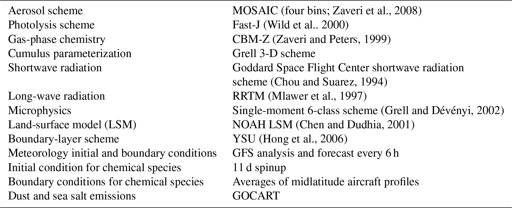
As in Chen et al. (2016), version 3.6.1 of the WRF-Chem model is used in this study to simulate the aerosols and gas-phase chemistry processes. A summary of the physical parameterizations used is given in Table 1. Details of the WRF-Chem model have been described by Grell et al. (2005) and Fast et al. (2006). The Carbon Bond Mechanism version Z (CBMZ) and MOSAIC schemes are used as the gas-phase and aerosol chemical mechanisms, respectively. The relative-humidity (RH)-dependent heterogeneous reactions added by Chen et al. (2016) are also applied in the simulations. The model computational domain covers most of China and its surrounding regions. Figure 1 presents the horizontal range of the domain, which contains 121×121 horizontal grids at a 40.5 km resolution. Vertically, there are 57 levels extending from the surface to 10 hPa.
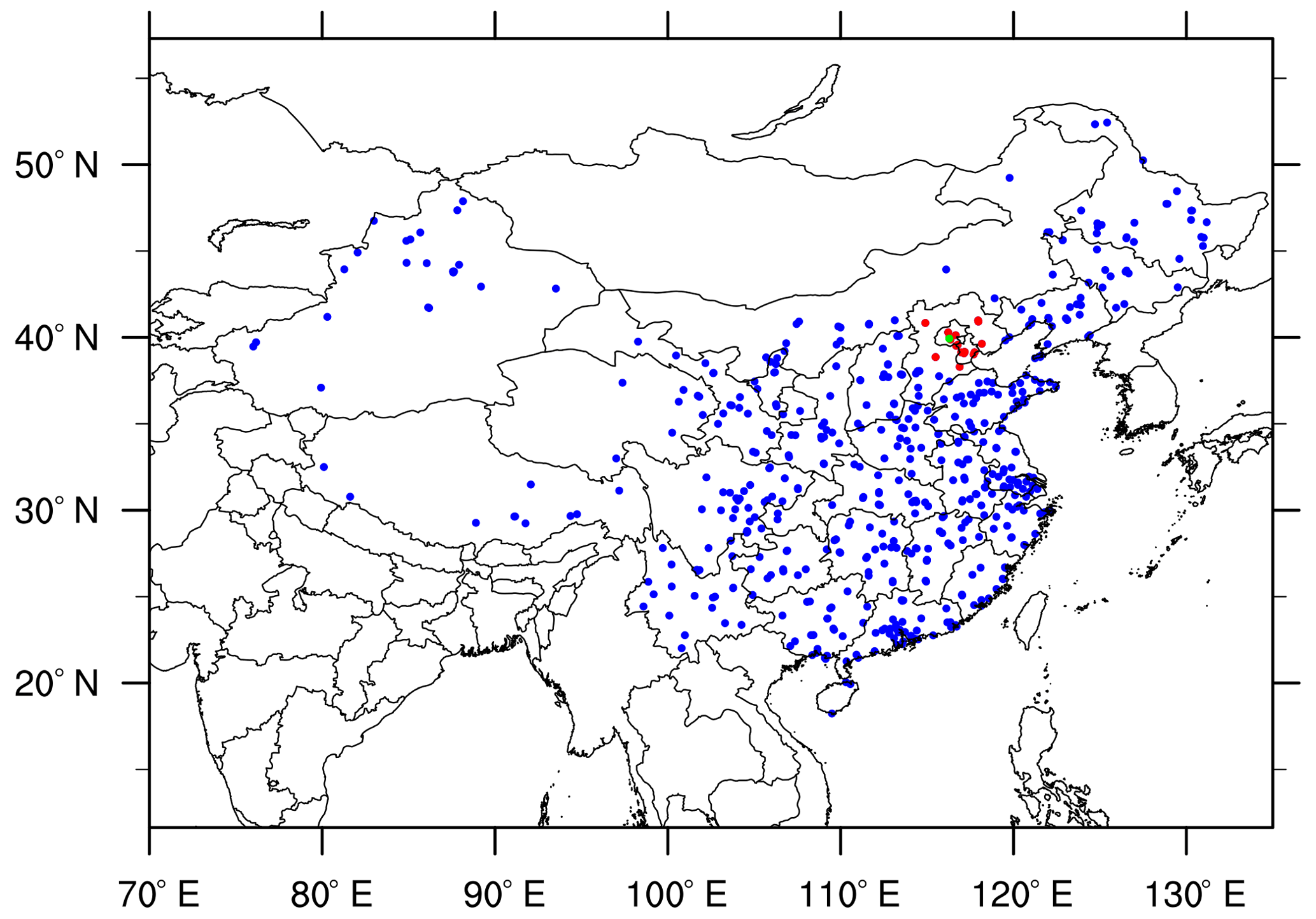
Figure 1Computation domain. Dots depict surface observations with 531 stations spreading over China. The red dots indicate the observations around Beijing. The green dot indicates the IUM station.
As in Chen et al. (2019), the emission input is based on the 2010 Multi-resolution Emission Inventory for China (MEIC) (He, 2012; Lei et al., 2011; Li et al., 2014; Zhang et al., 2009), which has already been applied in many recent studies over China (Wang et al., 2016; L. Wang et al. 2014; Zheng et al., 2015). The emission inventory has also been processed to match the model grid spacing (40.5 km) from an original grid spacing of (Chen et al., 2016). Admittedly, the difference between the emission base year and our simulation year and the spatiotemporal allocations may cause uncertainties in our simulation, this emission is the only publicly available emission inventory once the study is conducted. Meanwhile, the inhomogeneous spatial changes and large uncertainties in seasonal allocations of the emissions made it difficult to simply scale the original emission inventory for our study period (Chen et al., 2019).
The dust emission is the GOCART dust emission, and the biogenic emission is calculated online by the Gunther scheme within the WRF-Chem model. Given that the time period of this study (January) is not the period with large fires (crop or biomass burning), fire emission is not used in this study.
2.2 Observations
For the future application in the RMAPS-Chem operational air quality forecast system, the WRFDA-Chem system is designed to assimilate the hourly surface observations of six major pollutants (PM2.5, PM10, SO2, NO2, O3, and CO) from the China National Environmental Monitoring Center (CNEMC). To verify the capability of the system, we use the data for the whole month of January 2017. As in Chen et al. (2019), to perform statistical calculations, an observation dataset at 531 locations (Fig. 1) is acquired by averaging all the original observations (more than 1600 sites) that fall into the same model grid. Meanwhile, two steps of data quality control are conducted before DA. Firstly, observations larger than a threshold are treated as unrealistic and are not assimilated. Secondly, observations leading to innovations (observations minus the model-simulated values) higher than a maximum deviation are omitted. For PM2.5, PM10, SO2, NO2, O3, and CO, the threshold in the first step is 500, 700, 200, 200, 200, and 20 mg m−3, respectively; the maximum deviation in the second step is 120, 120, 60, 60, 60, and 6 mg m−3, respectively.
To verify sulfate–nitrate–ammonium partitioning, a site observation of different chemical species is used in Sect. 4. The measurements were performed over 14–20 January 2017, and carried out on the roof of IUM in Beijing (green dot in Fig. 1). A detailed description of the features of the observation, including the quality assurance and quality control, has been given by Su et al. (2018). This study mainly uses the sulfate () and nitrate () in this dataset.
2.3 WRFDA-Chem system
In this study, an aerosol or chemical assimilation capability is built within the version 4.0.3 of the WRFDA system with the 3DVAR algorithm. The WRFDA 3DVAR produces the analysis through the minimization of a scalar objective function J(x) given by
where xb denotes the background vector, y is a vector of the observations, and B and R represent the background and observation error covariance matrices, respectively. The covariance matrices determine how closely the analysis is weighted toward the background and observations. H is the observation operator that interpolates model grid point values to observation space and converts model-predicted variables to observed quantities.
Generally, the implementation of WRFDA-Chem 3DVAR includes several parts: the WRF-Chem model and surface air pollutant observation interface to WRFDA, the addition of aerosol or chemical analysis variables, the surface air pollutant observation operators, the update of observation errors, and the statistics of background error covariances for chemical analysis variables. Detailed descriptions will be presented in the following parts. It is worth mentioning that the new WRFDA-Chem system is designed with a flexible aerosol assimilation capability that can switch between different aerosol schemes. Given the fact that the WRF-Chem model predicts the PM concentrations in the forms of different prognostic variables depending on the aerosol scheme chosen, the aerosol or chemical prognostic variables are given in the registry file of the WRFDA-Chem instead of being specifically defined in the code. With the help of the registry mechanism of the WRF model, the prognostic variables in the entire DA process can be easily adjusted by modifying the registry file. The WRFDA-Chem system has been tested with GOCART and the MOSAIC aerosol scheme, while this study focuses on the MOSAIC scheme.
2.3.1 Observation operators
The WRFDA-Chem is designed to assimilate six types of surface aerosol or chemical observations, including PM2.5, PM10, SO2, NO2, O3, and CO. For aerosol assimilation, the aerosol species in the MOSAIC scheme are defined as black carbon (BC), organic compounds (OCs), sulfate (), nitrate (), ammonium (), sodium (Na), chloride (Cl), and other inorganic compounds (OINs). To represent the aerosol size distribution, MOSAIC uses a sectional approach with different bins. This study uses four size bins with aerosol diameters ranging from 0.039 to 0.1, 0.1 to 1.0, 1.0 to 2.5, and 2.5 to 10 µm. The PM2.5 total is controlled by the 24 variables in the first three bins (eight species multiplied by three bins), and the PM10 total is controlled by the 32 variables in the four bins (eight species multiplied by four bins). As a result, the model-simulated PM2.5 is computed by summing the 24 variables as
The model-simulated PM10 observations are computed by summing the 32 variables as
Correspondingly,
where ρd is the dry-air density, which is used to convert the unit of the analysis variable (µg kg−1) to the observations (µg m−3); i denotes the bin number in the MOSAIC aerosol scheme. In the experiment assimilating PM2.5 alone, the PM2.5 observations are used to analyze the species in the first three bins (Eq. 2). In the experiment assimilating PM2.5 and PM10 simultaneously, the PM2.5 observations are used to analyze the species in the first three bins (Eq. 2), and the PM10–2.5 (PMcoarse, hereafter) in the observations is used to analyze the species in the fourth bin (Eq. 4). A similar approach has been adopted by Peng et al. (2018).
In the assimilation of the gas-phase pollutants, the model-simulated values are computed by
where x denotes the four gas-phase pollutants SO2, NO2, O3, and CO, ρd is the dry-air density, Mx is the relative molecular mass for the four gas-phase pollutants, Mdair is the relative molecular mass for dry-air, and Rx is the mixing ratio for the four gas-phase pollutants. Since the gas-phase pollutant observations are mass concentrations in micrograms per cubic meter and the analysis variables are mixing ratios in parts per million by volume, Eq. (5) is used for the unit conversion.
2.3.2 Observation errors
Following Chen et al. (2019) and Peng et al. (2018), the observation error covariance matrix R in Eq. (1) is estimated from measurement error ε0 and the representativeness error εr in this study. The measurement error ε0 is defined as , where Mi denotes the observation of the six major pollutants in micrograms per cubic meter; the representativeness error εr is defined as , where γ is an adjustable parameter scaling (set as 0.5), Δx is the grid spacing (40.5 km in our case), and L is the radius of influence of the observation (set to 2 km). These parameter settings are based on the sensitivity tests by Chen et al. (2019). The total observation error (εx) is computed as , where x denotes the six major pollutants PM2.5, PM10, SO2, NO2, O3, and CO.
2.3.3 Background error covariance
To implement the aerosol or chemical DA with the MOSAIC four-bin scheme, this study expands GEN_BE v2.0 (Descombes et al., 2015) to compute the B matrix in Eq. (1) for the 32 chemical variables as in Eq. (3) (BC, OC, , , , Na, Cl, and OIN in four bins), as well as the four gas-phase variables as in Eq. (5) (SO2, NO2, O3, and CO). Since it is both technically and scientifically challenging to model the cross-correlations between different aerosol or chemical variables in a 3DVAR framework, they are not considered in this study. We plan to introduce the cross-variable correlations with the ensemble-variational approach in the future extension of the system. With the updated GEN_BE v2.0, the statistics for background error covariance, such as standard deviation, vertical and horizontal length scales, and vertical correlations, are computed for each of the aerosol or chemical variables. In this study, the background error covariance is estimated using the National Meteorological Center (NMC) method (Parrish and Derber, 1992) from 1-month WRF-Chem forecasts over January 2017.
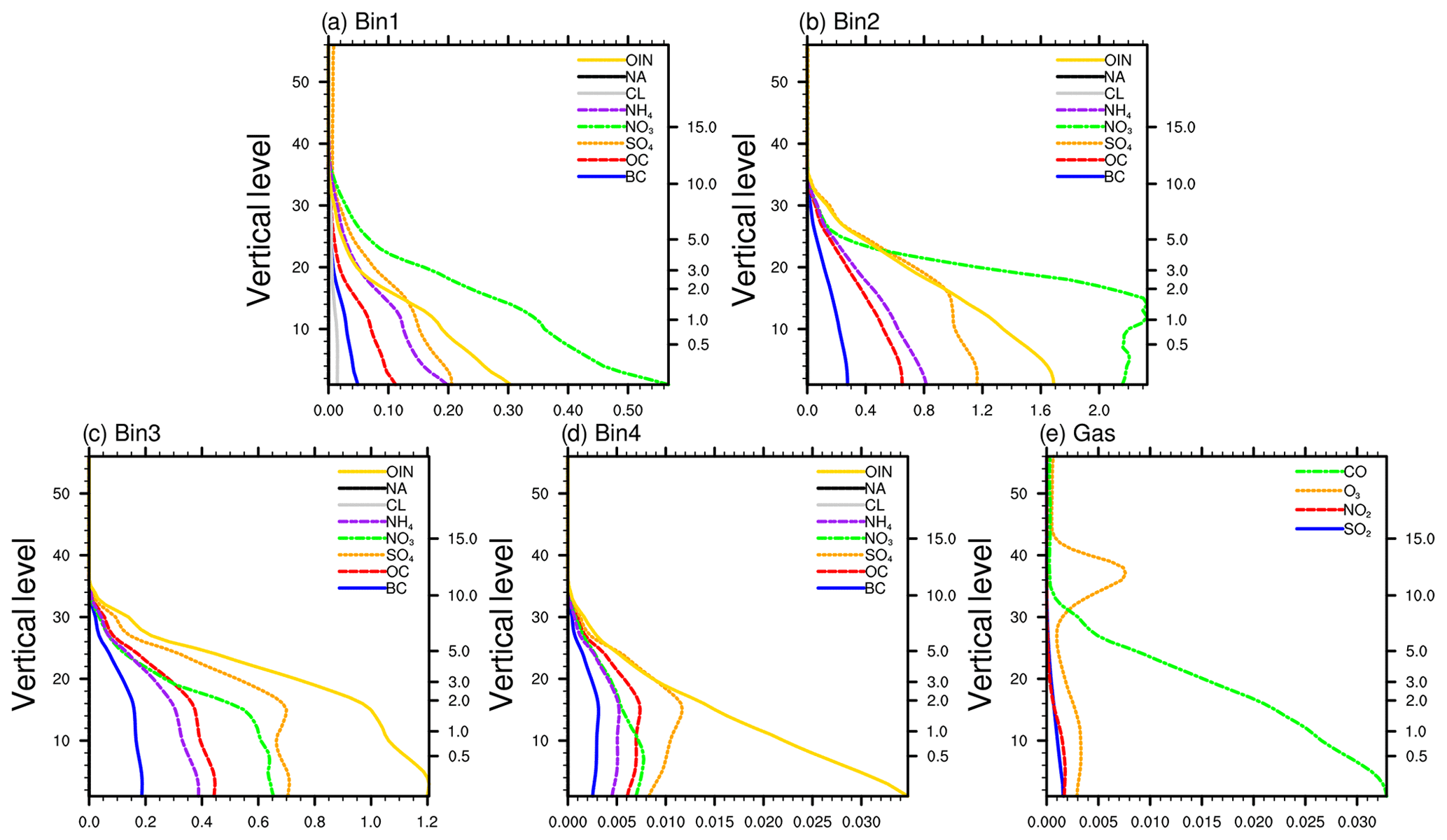
Figure 2Background error standard deviations of aerosol species of the (a) first size bin, (b) second size bin, (c) third size bin, (d) fourth size bin, and (e) gas pollutants. The units for the x axis are micrograms per cubic meter for (a–d) and parts per million for (e). The left y axis denotes the model level, and the right y axis denotes the vertical height (units: km).
Following the analyses based on GEN_BE v2.0 (Descombes et al., 2015), Fig. 2 presents the background error standard deviations of each species at different vertical levels. For the aerosols in the first three size bins (Fig. 2a–c), although the standard deviation errors vary across the species, the errors of , , , OC, and OIN are generally larger than those of the others (BC, Cl, and Na) in the three size bins. These results are consistent with the finding in Chen et al. (2019), which allows inorganic compounds (, , ), OC, and OIN to be adjusted more corresponding to their larger background errors. For the aerosols in the fourth size bin (Fig. 2d), the errors are unreasonably much smaller than in the first three bins due to model deficiency. Under these circumstances, to obtain a reasonably larger adjustment for the aerosols in the fourth size bin, it might be necessary to enlarge their background errors in the DA procedure. As for the gaseous pollutants (Fig. 2e), CO has the largest background errors in the middle and lower layers, followed by O3, SO2, and NO2.
For the background error horizontal correlation length scales, the results are similar to those in Liu et al. (2011) (figure omitted). The length scales of aerosols are comparable in most of the species, which generally span from 1.5 to 2.5 times the grid spacing, while the aerosol species Na shows a smaller horizontal length scale than all the other species. For the background error vertical correlations (figure omitted), the results are similar to those in Descombes et al. (2015), in which the vertical correlations are larger in the lower levels (where they are emitted) in most of the species. According to Descombes et al. (2015), the reactions with species emitted near the surface might create these strong correlations in the lower model levels.
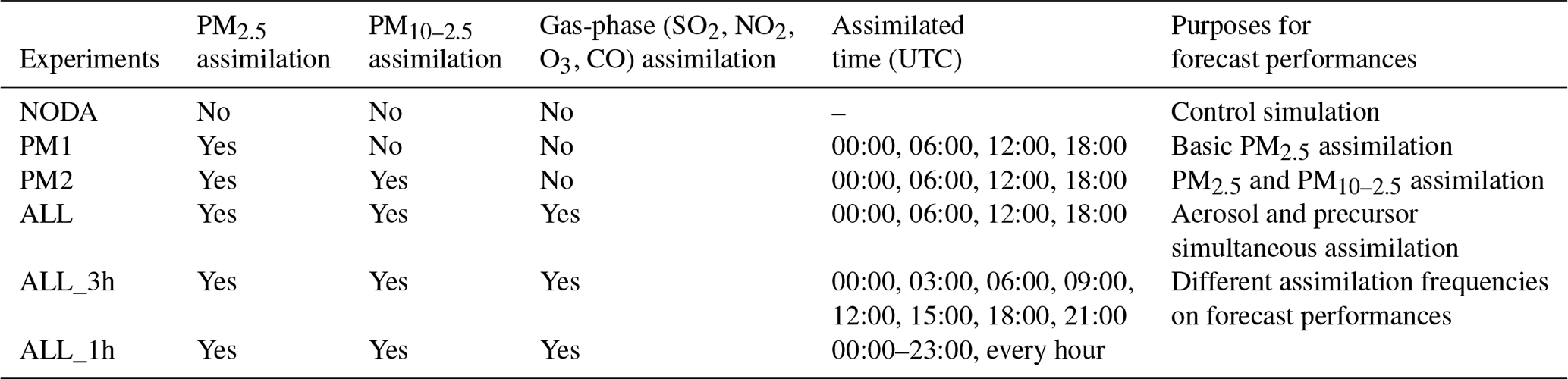
Table 2Detailed setting of six experiments and their purposes.
2.3.4 Experimental design
To seek for the best forecast performance, six experiments were conducted for January 2017 in this study: NODA, PM1, PM2, ALL, ALL_3h, and ALL_1h (detailed in Table 2). NODA is the control experiment without any data assimilation. The design of PM1, PM2, and ALL is to investigate the assimilation impacts of PM2.5, PMcoarse, and gas-phase pollutants (SO2, NO2, O3, CO) step by step.
The NODA experiment initialized a new WRF-Chem forecast every 6 h between 00:00 UTC, 20 December 2016, and 18:00 UTC, 31 January 2017, in which the aerosol or chemical fields were simply carried over from cycle to cycle, and the meteorological initial condition or boundary conditions were updated from GFS (Global Forecast System) data every 6 h. The first 10 d were treated as the spinup period, and only simulations in January were used in the following analyses. The PM1, PM2, and ALL experiments updated the chemical initial condition (IC) using the WRFDA-Chem system every 6 h starting from 00:00 UTC, 1 January. The background of the first cycle was obtained from the NODA experiment, and all subsequent cycles were derived from the 6 h forecast of the previous cycle. The only difference between PM1, PM2, and ALL experiments is that PM1 only assimilated PM2.5 observations; PM2 assimilated PM2.5 and PMcoarse (PM10–2.5) simultaneously; ALL assimilated PM2.5, PM10–2.5, SO2, NO2, O3, and CO together.
In view of the cycling frequency being an important aspect in the DA strategy, especially for 3DVAR, two more experiments that assimilate all the six major pollutants with a 3 and 1 h cycling frequency were conducted (experiments ALL_3h and ALL_1h). To investigate the forecast improvements, a 24 h forecast was initialized for all the experiments at 00:00 UTC of each day.
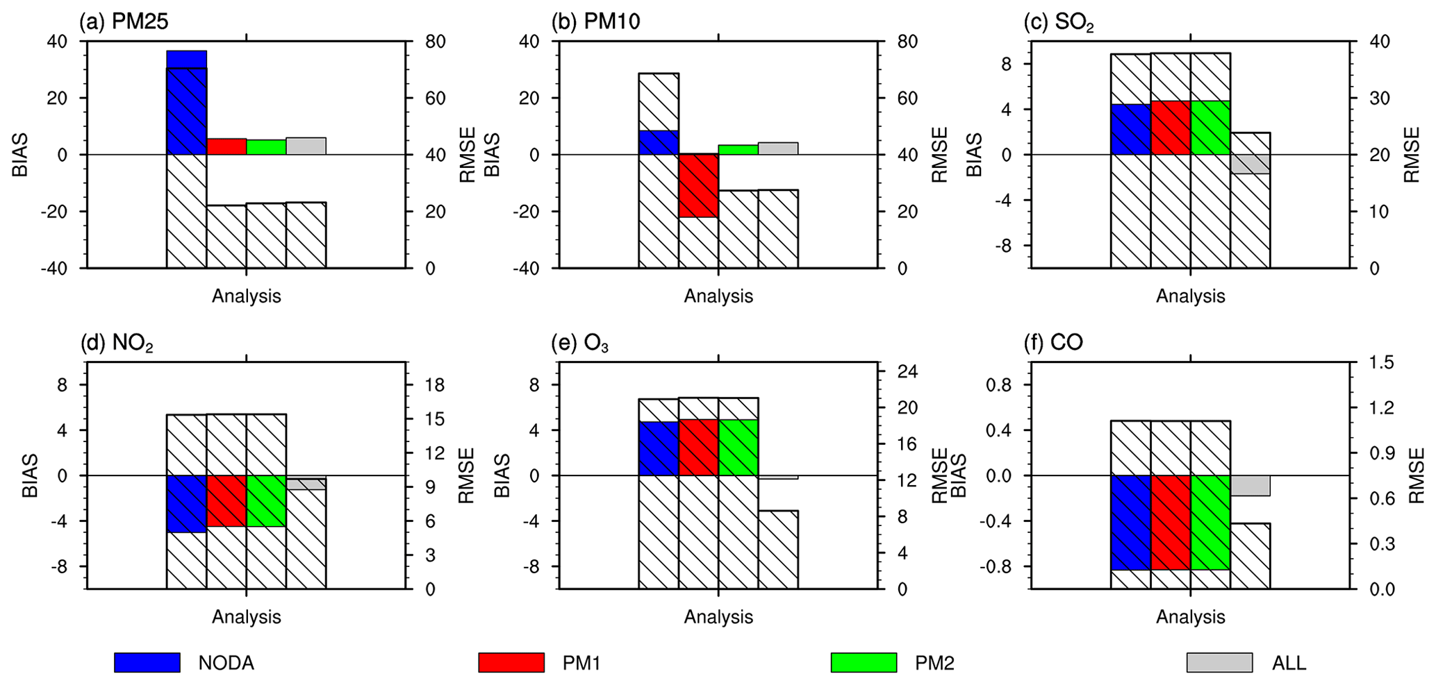
Figure 3Averaged bias (colored bar, left y axis) and RMSE (hollow bar, right y axis) of the analysis at 00:00 UTC over 1–31 January 2017 for (a) PM2.5, (b) PM10, (c) SO2, (d) NO2, (e) O3, and (f) CO in different experiments, verified against the surface observations of 531 stations in China. The blue, red, green, and gray shaded bars denote the bias of the experiments NODA, PM1, PM2, and ALL, respectively; the corresponding hollow bars denote the RMSE of these experiments. Units of the y axis are micrograms per cubic meter in (a–e) and milligrams per cubic meter in (f).
3.1 Impact on analyses
To evaluate the performance of the WRFDA-Chem system, the impact on analyses is firstly investigated. Figure 3 presents the domain-averaged bias and root-mean-square-error (RMSE) of the analysis at 00:00 UTC over 1–31 January 2017. For PM2.5 (Fig. 3a), the NODA experiment displays a general overestimation of 36.60 µg m−3, along with a large RMSE of 70.41 µg m−3. After DA, in the PM1, PM2, and ALL experiments, the bias of PM2.5 drops to 5.62, 5.19, and 5.98 µg m−3, respectively; the RMSE drops to 22.10, 22.84, and 23.15 µg m−3, respectively.
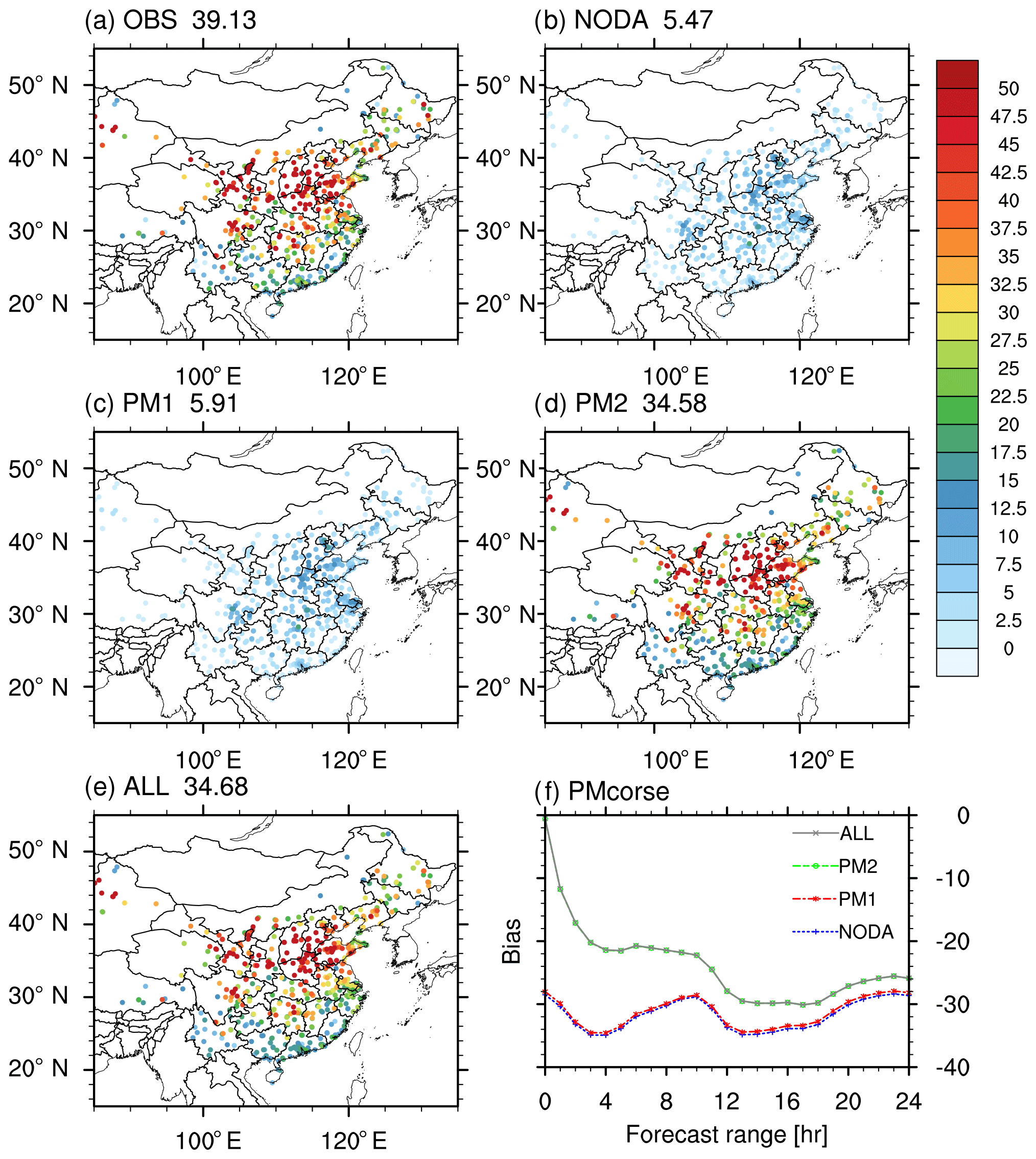
Figure 4Averaged PMcoarse (PM10–2.5; units: µg m−3) at 00:00 UTC over 1–31 January 2017 in (a) observation and the four experiments (b) NODA, (c) PM1, (d) PM2, (e) ALL, and (f) averaged bias (units: µg m−3) for PMcoarse in different experiments as a function of forecast range (the blue, red, green, and gray lines denote the results of experiment NODA, PM1, PM2, and ALL, respectively), verified against the surface observations of 531 stations in China. The numbers at the top of each panel denote the average PMcoarse concentrations over 531 stations (units: µg m−3).
In the analyses of PM10, it is noted that the PM1 experiment has a larger bias than the NODA run (Fig. 3b). To explain this phenomenon, Fig. 4 presents the monthly mean difference between PM10 and PM2.5 (PM10 minus PM2.5, PMcoarse) in the analysis. In the observation, PMcoarse generally increases from south to north, reaching above 50 µg m−3 over northern China (Fig. 4a). However, PMcoarse in the NODA experiment (with an average of 5.47 µg m−3) is much smaller than that in the observation (with an average of 39.13 µg m−3). This result suggests that the WRF-Chem model failed to reasonably represent PMcoarse, which is actually the fourth bin of the aerosol species in the MOSAIC scheme. Under these circumstances, when the assimilation of PM2.5 tries to reduce its evident overestimation (Fig. 3a), components in the first three bins (within 2.5 µm) of PM10 decrease dramatically. Meanwhile, since the simulated PMcoarse is too small, the PM10 variates are eventually dominated by the adjustment of PM2.5. As a result, the assimilation of PM2.5 causes a large negative bias in the PM10 analysis (Fig. 3b). Correspondingly, compared to the NODA run, PMcoarse in the PM1 experiment shows no significant changes (only a slight decrease) in the analysis (Fig. 4b and c) and also in the forecast (Fig. 4f).
To overcome this issue, several adjustments have been adapted in the PM10 assimilation: instead of using the PM10 observations directly, PMcoarse is used to analyze the species in the fourth bin (Eq. 4); to reflect the large uncertainty of the simulated PMcoarse and to appropriately weight the model and observation errors, the background error covariance of PMcoarse (species in the fourth bin) is arbitrarily inflated (inflation factor 1 is normally used and 90 is selected after tuning). By these means, after assimilating the PM10 observations, the PM2 and ALL experiments show similar distributions in PMcoarse (Fig. 4d–e, with an average of 34.58 and 34.68 µg m−3) as in the observation (with an average of 39.13 µg m−3). Correspondingly, compared to the NODA experiment, evident improvements for PM10 analysis appear in the PM2 and ALL experiments, in which the bias and RMSE drops noticeably (Fig. 3b). Overall, the DA experiments show strong contributions to the analyses of PM2.5 and PM10, suggesting that the WRFDA-Chem system works effectively in updating the initial conditions.
As for the analyses of gaseous pollutants (Fig. 3c–f), large improvements can be seen in the ALL experiment by further assimilating SO2, NO2, O3, and CO. Compared to the PM2 experiment, although the bias and RMSE for PM2.5 and PM10 in the ALL experiment are slightly larger, the bias for the four gaseous pollutants decreases from 4.74, −4.59, 4.92, and −8.31 mg m−3 (PM2 experiment) to −1.68, −1.25, −0.31, and −0.18 mg m−3 (ALL experiment), respectively, and the corresponding RMSE drops from 37.87, 15.39, 21.04, and 1.11 mg m−3 (PM2 experiment) to 23.85, 9.70, 8.62, and 0.43 mg m−3 (ALL experiment). In general, by assimilating all the six major pollutants, the ALL experiment displays the largest improvement in the analyses of gaseous pollutants among all the experiments, along with a comparable improvement in the analyses of the aerosols.
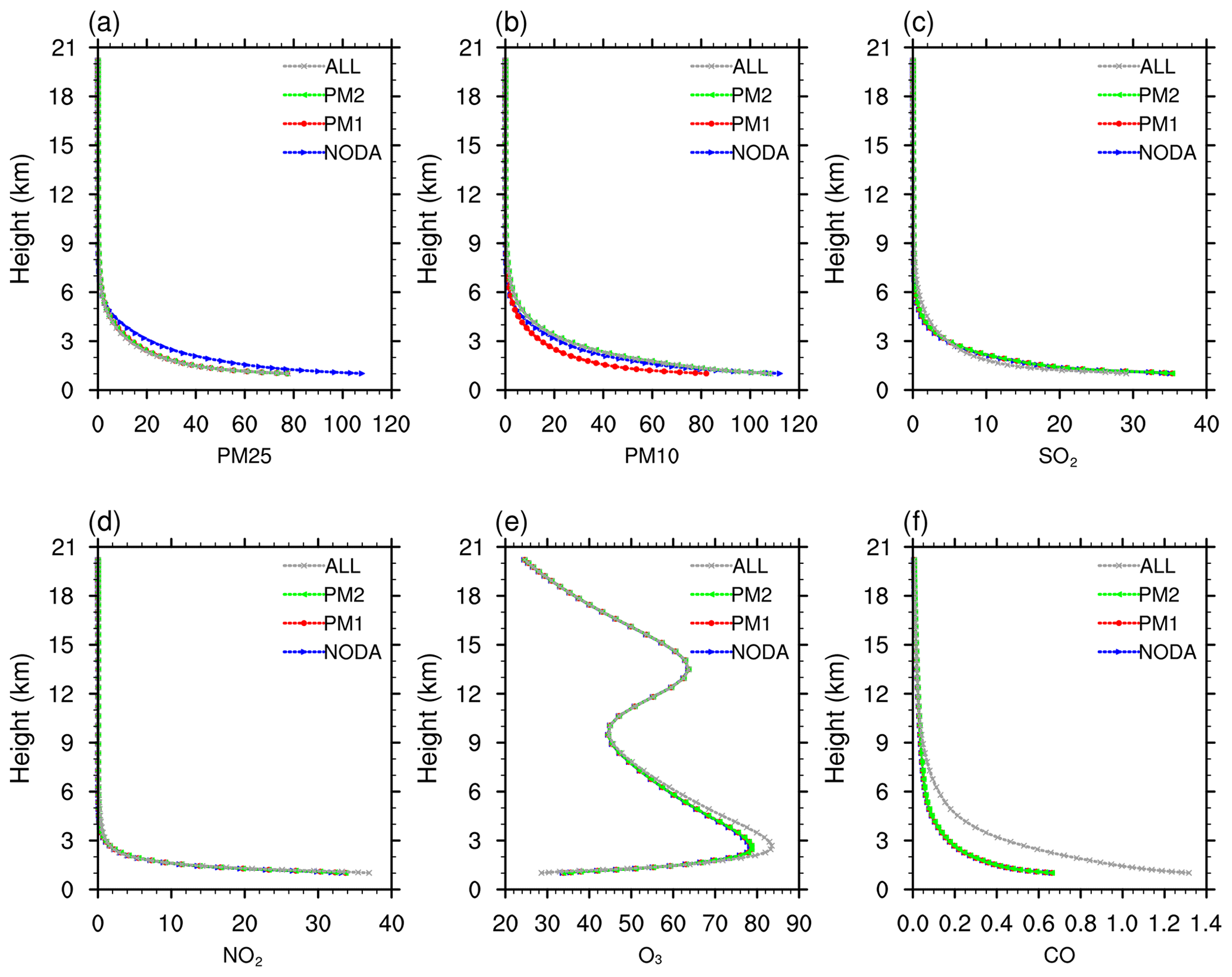
Figure 5Vertical profile of the analysis at 00:00 UTC over 1–31 January 2017 for (a) PM2.5, (b) PM10, (c) SO2, (d) NO2, (e) O3, and (f) CO in different experiments, averaged over the 531 surface stations in China. The blue, red, green, and gray lines denote the results of experiment NODA, PM1, PM2, and ALL, respectively. Units of the y axis are micrograms per cubic meter in (a–e) and milligrams per cubic meter in (f).
Due to the lack of vertical information within the observations, the common mathematical solution to use the surface total mass observations to analyze multiple 3-D fields variables is to utilize prior information in the background. As shown in Fig. 5, based on vertical correlations specified in the background error covariance, the observation impact spreads to a certain height, even though the analysis variables used in the observation operator (Eqs. 2–5) are only at the lowest model level. It is also noted that observations contribute differently to the analysis variables. Corresponding to the strong overestimation of PM2.5 (Fig. 3a), all the three DA experiments (PM1, PM2, and ALL) tend to reduce the PM2.5 below 6 km; corresponding to the distinct underestimation for CO (Fig. 3f), the experiment assimilating CO (ALL experiment) increases the value below 9 km. Relatively small analysis increments are shown in the other three gas pollutants (SO2, NO2, and O3).
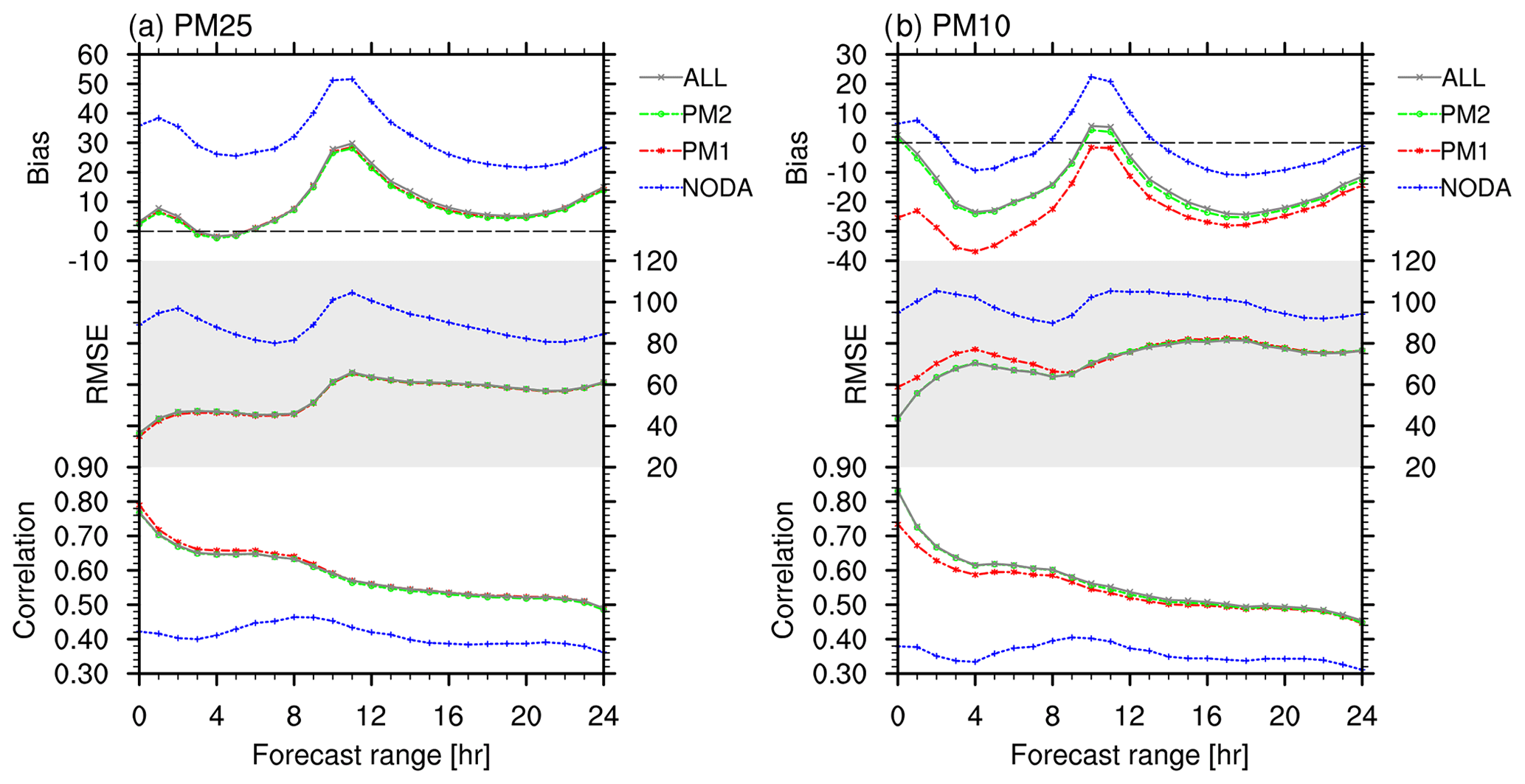
Figure 6Averaged bias (units: µg m−3), RMSE (units: µg m−3), and correlation for (a) PM2.5 and (b) PM10 in different experiments as a function of forecast range, verified against the surface observations of 531 stations in China. The blue, red, green, and gray lines denote the results of experiment NODA, PM1, PM2, and ALL, respectively.
3.2 Forecast improvements
After illustrating the effect of WRFDA-Chem on the analyses, this section further investigates the forecast performances based on the new analyses. A 24 h forecast is performed at each 00:00 UTC from 1 to 31 January 2017. The forecast error statistics, including bias, RMSE, and correlation, are computed by verifying them against the surface observations at 531 stations over China.
Table 3Averaged bias (units: µg m−3), RMSE (units: µg m−3), and correlation over forecast hours 0–24 h for different variables and different experiments. The statistics for gas-phase pollutants in PM1 and PM2 experiments are very close to the results in the NODA experiment and thus are left blank in the table.
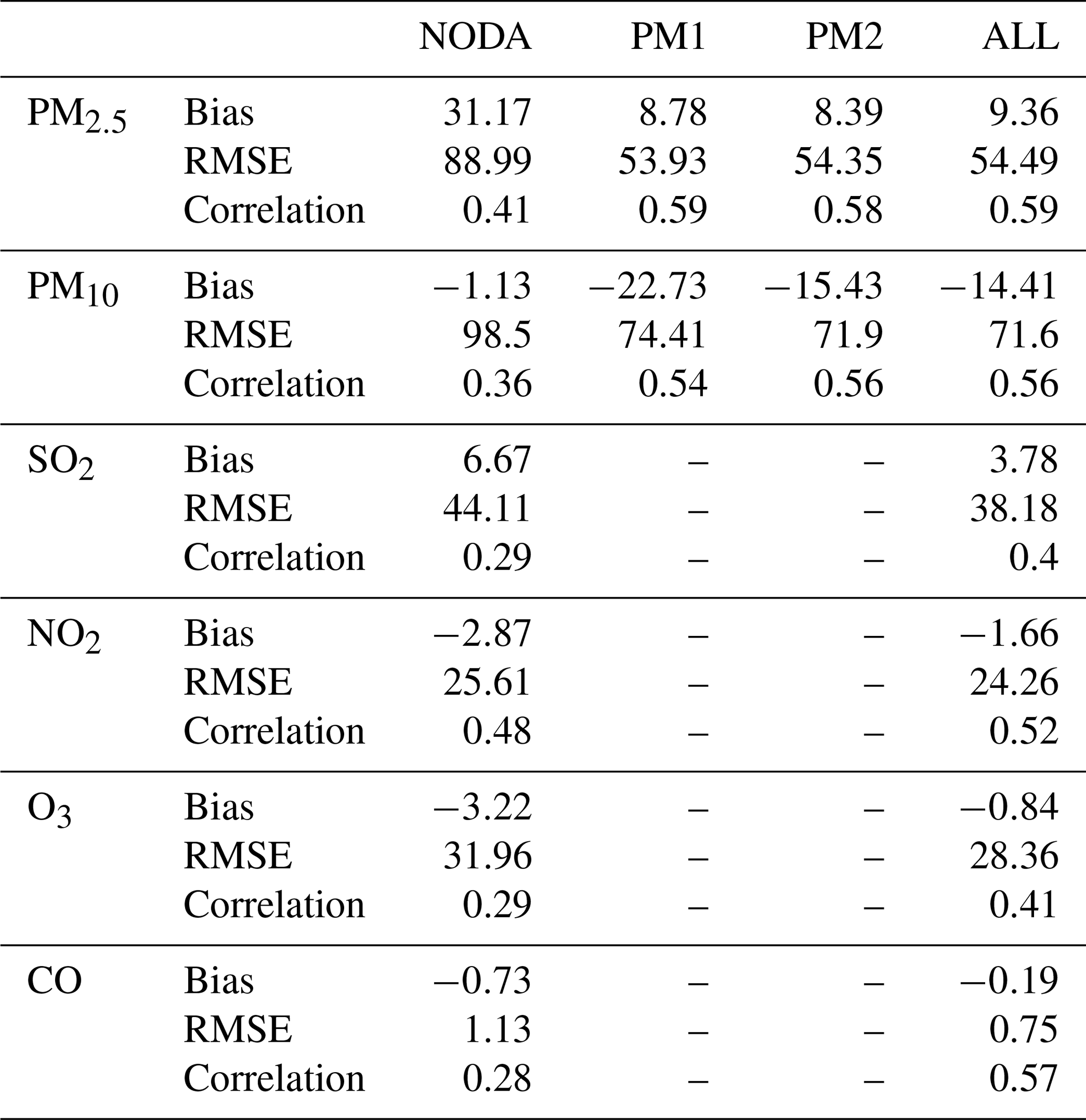
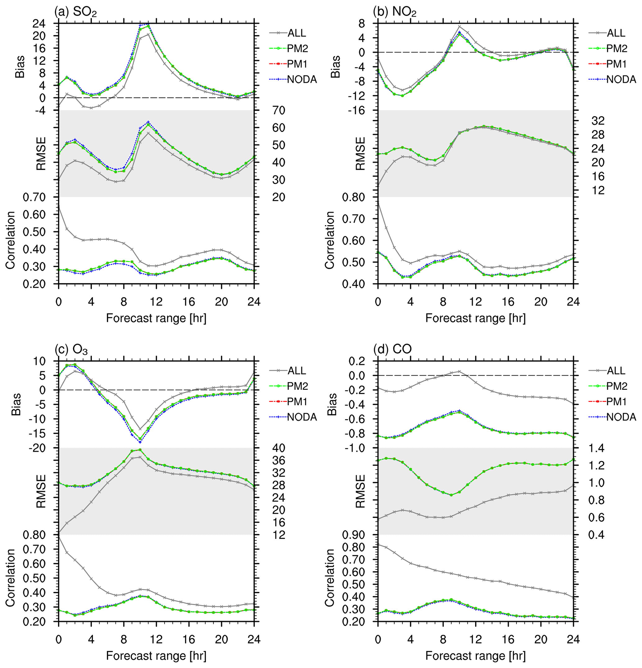
Figure 7Same as Fig. 6, but for the forecast of (a) SO2, (b) NO2, (c) O3 (units: µg m−3), and (d) CO (units: mg m−3).
As shown in Fig. 6, the model performs relatively poorly in the forecast of aerosols without DA. For PM2.5, the average bias, RMSE, and correlation over 0–24 h are 31.17, 88.99, and 0.41 µg m−3, respectively (Table 3). As expected, all the DA experiments evidently improve the forecasts. Along with the forecast range, distinct improvements in bias, RMSE, and correlation last from 0 to 24 h. For example, in the PM1 experiment, the average improvement percentages (over 0–24 h) for bias, RMSE, and correlation reach up to 71.8 %, 39.4 %, and 43.9 %, respectively. It is also noted that the PM2.5 observation is the dominant data source in improving PM2.5 forecast. As for PM10, distinct improvements in RMSE and correlation can be seen from 0 to 24 h. Especially after assimilating PMcoarse (PM10–2.5 in PM2 and ALL experiments), the averaged improvement percentage for RMSE and correlation reach up to about 27.0 % and 55.5 %. For bias, since the statistics are averaged over the 531 stations, the offset of large positive and negative bias at different stations leads to the small averaged bias in the NODA run (see the spatial distribution of bias at the individual site in Sect. S1 of the Supplement). Considering that the DA experiments show distinct improvements in RMSE and correlation, WRFDA-Chem still provides a generally positive contribution to the PM10 forecast.
Figure 7 presents the averaged forecast error statistics for SO2, NO2, O3, and CO with respect to the forecast range. In PM1 and PM2 experiments that do not assimilate the gas-phase observations, no significant changes appear in the forecasts of the gaseous pollutants compared to the NODA run; after assimilating the gas-phase observations, the ALL experiment shows evident improvements in all the four gaseous pollutants, in which the improvements for SO2, NO2, and O3 are more significant in 0–10 h, and the improvements for CO last up to 24 h. According to the numbers shown in Table 3, for SO2, NO2, O3, and CO, the average bias (RMSE) in the ALL experiment decreases by 43.3 %, 42.2 %, 73.9 %, and 74.0 % (13.4 %, 5.3 %, 11.3 %, and 33.7 %), compared to the NODA run, and the average correlation increases by 37.9 %, 8.3 %, 41.4 %, and 103.5 %, respectively. It is worth noting that the WRFDA-Chem system has a positive impact on the forecast of NO2 and O3 by merely analyzing the IC. Since NO2 and O3 are related to complex photochemical reaction processes, the assimilation of NO2 and O3 usually does not work as well as other gas-phase pollutants for the forecast aspect, even with both emission and IC analyzed (Peng et al., 2018). As a result, the aerosol or chemical assimilation based on WRFDA-Chem could not only contribute to the conventional aerosol forecasts in operational applications but also provide valuable help in the emerging study demands for gaseous pollutants, especially O3.
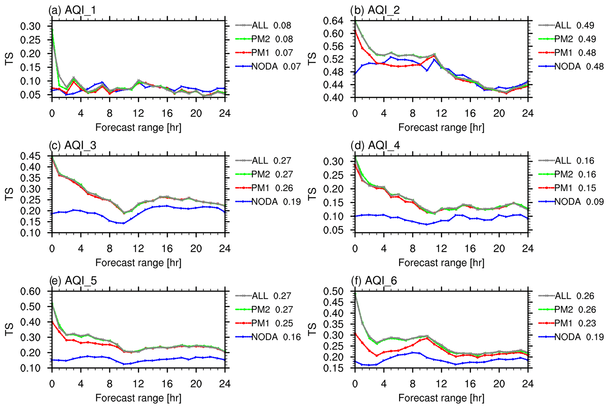
Figure 8Averaged threat score (TS) for the Air Quality Index (AQI) from AQI level 1 to level 6 (a–f) in different experiments as a function of forecast range, verified against the surface observations of 531 stations in China. The blue, red, green, and gray lines denote the results of experiment NODA, PM1, PM2, and ALL, respectively. The numbers to the right of each panel denote the averaged TS from 0 to 24 h for different experiments.
The Air Quality Index (AQI), which is used for reporting daily air quality and issuing alarms, is one of the service products of RMAPS-Chem operational air quality model over northern China. Generally, AQI is classified into six level ratings from good to hazardous: 0–50 (level 1), 51–100 (level 2), 101–150 (level 3), 151–200 (level 4), 201–300 (level 5), and 300+ (Level 6). Similar to previous studies (Kumar and Goyal, 2011; Tao et al., 2015; Zheng et al., 2014), AQI is calculated for the six major pollutants. The pollutant with the highest AQI level is deemed to be the “main pollutant” and its AQI determines the overall AQI level. Accordingly, the accurate forecast of AQI requires the overall good performances of the six pollutants. To reflect the integrated DA effect of aerosols and gas-phase pollutants, the threat score (TS), one of the most commonly used criteria in the verification of meteorology forecasting, is used for AQI at each AQI level. The TS for the AQI is calculated by
where H, M, and F denote the times of the hits, the misses, and the false alarms in the forecast of AQI and i denotes the AQI levels from 1 to 6. As a result, the TS is acquired at each AQI level ranging from 0 to 1, and the higher (lower) TS represents the better (worse) forecast performance.
As shown in Fig. 8, in the beginning of the forecast, DA experiments (PM1, PM2, and ALL) increase the TS remarkably at all AQI levels, and it then gradually decreases (quickly drops) with the forecast range at AQI levels 2–6 (AQI level 1). Nevertheless, for the polluted situations with AQI levels 3–6, evident improvements can be seen from 0 to 24 h in all the DA experiments, in which the average TS increases from 0.19, 0.09, 0.16, and 0.19 (NODA experiment) to about 0.27, 0.16, 0.27, and 0.26 (DA experiments), respectively. For heavily polluted situations with AQI levels 5–6 (Fig. 8e–f), compared to the PM1 case, TS experiences a further increase in the PM2 and ALL experiments after assimilating PMcoarse (PM10–2.5). This result indicates that for heavily polluted events during this period (January 2017), PM2.5 and PM10 could be the main pollutant that contributes the most to the AQI.
In general, the new WRFDA-Chem evidently improves the aerosol or chemical forecasting. Based on the assimilation of the six major pollutants, the chemical ICs are improved distinctly and a better forecast performance is acquired up to 24 h. Among the different experiments, the ALL experiment displays the best forecast error statistics for most of the major pollutants along with the highest TS for AQI. In the following operational applications, it is recommended to assimilate the six major pollutants simultaneously, which will help to obtain better analyses and forecast skills on the whole.

Figure 9Same as Fig. 3, but for the experiments of NODA, ALL_6h, ALL-3h, and ALL_1h, respectively. Units of the y axis are micrograms per cubic meter in (a–e) and milligram per cubic meter in (f).
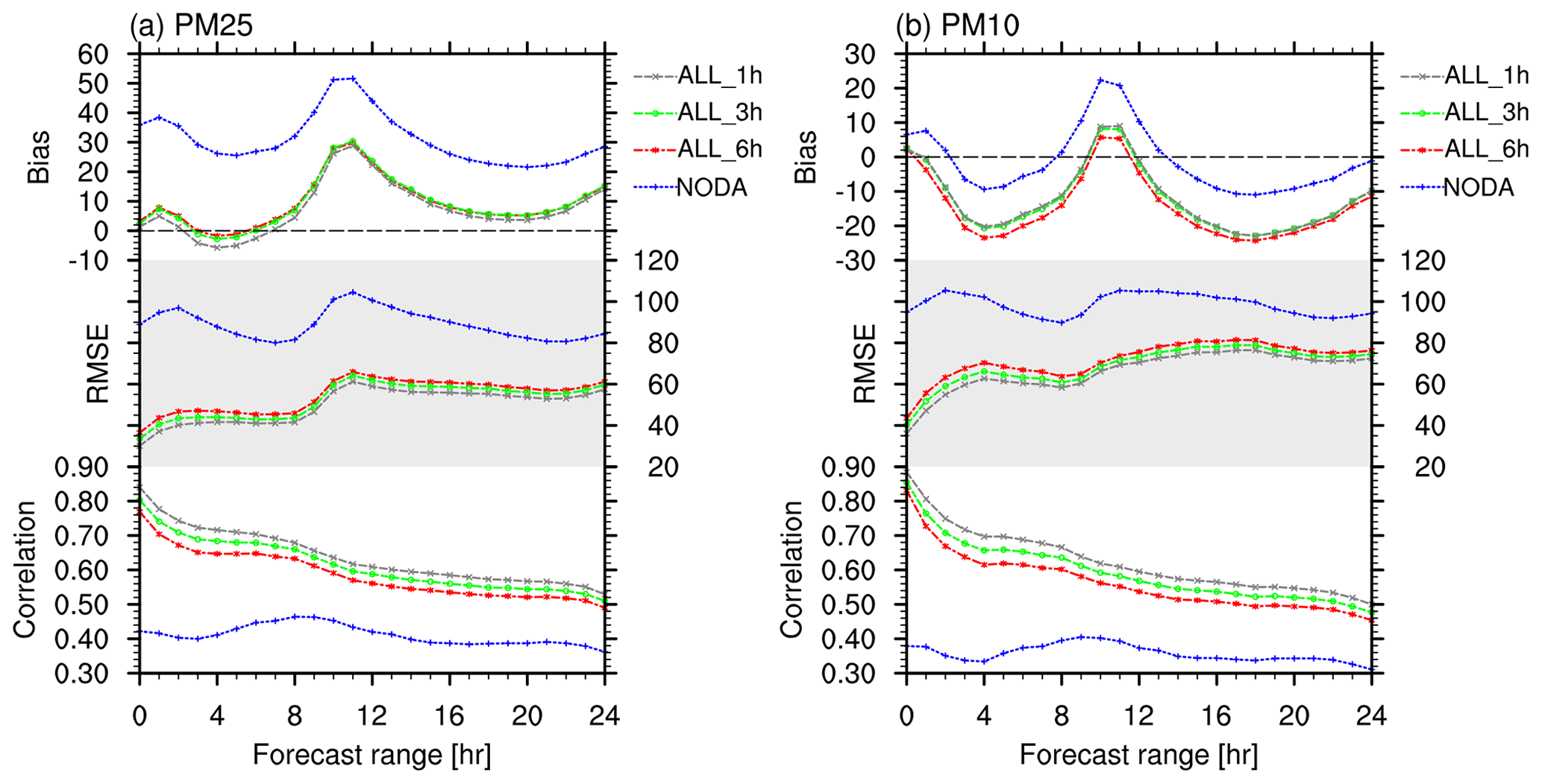
Figure 10Averaged bias (units: µg m−3), RMSE (units: µg m−3), and correlation for (a) PM2.5 and (b) PM10 in different experiments as a function of forecast range, verified against the surface observations of 531 stations in China. The blue, red, green, and gray lines denote the results of experiment NODA, ALL_6h, ALL_3h, and ALL_1h, respectively.
3.3 Response to DA cycling frequency
Cycling frequency is an important aspect in the DA strategy. However, the responses toward IC updating could be different among the pollutants. To work out this issue and to provide helpful references for future applications, DA experiments with different cycling frequencies were analyzed in this section.
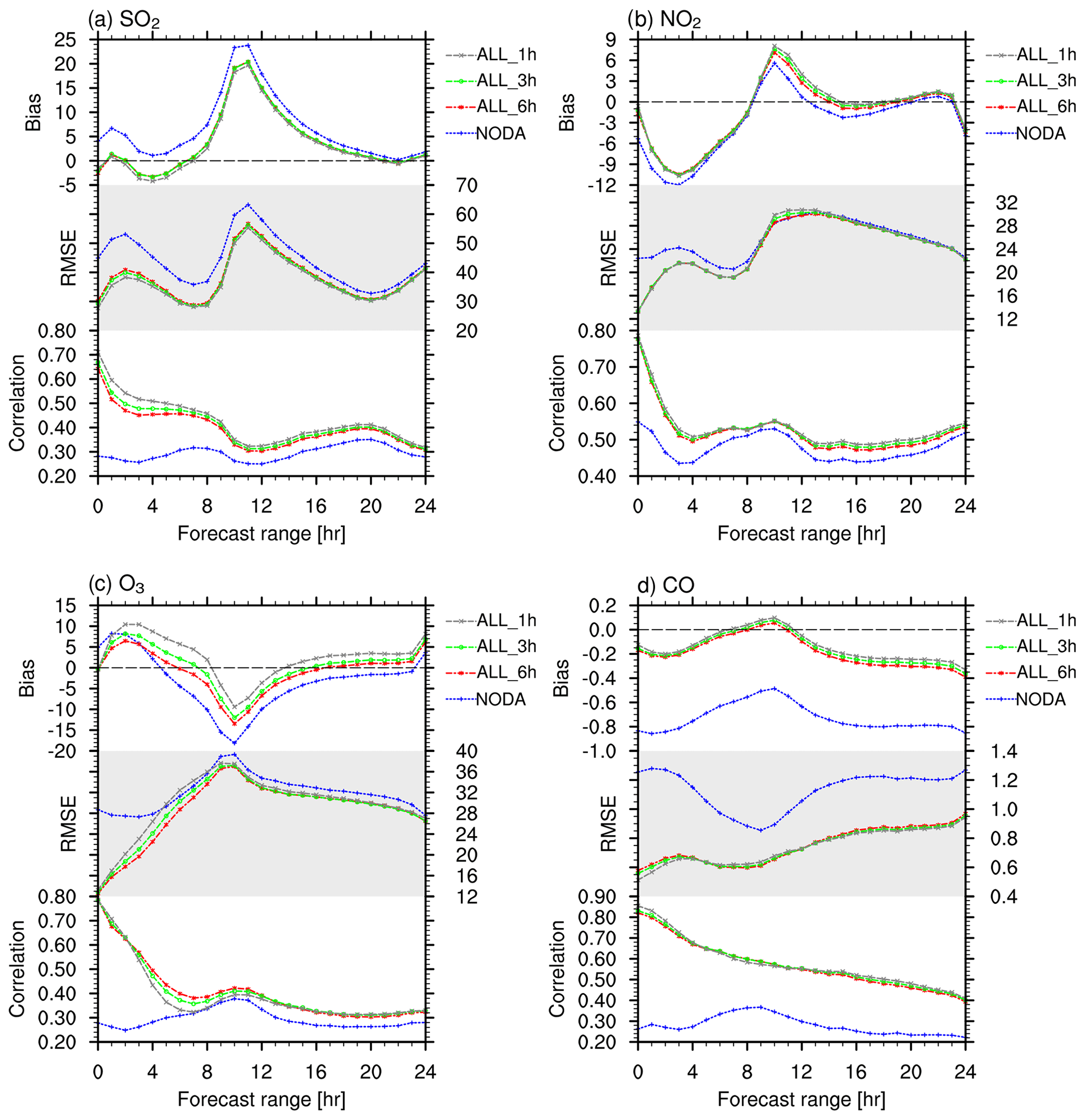
Figure 11Same as Fig. 10, but for the forecast of (a) SO2, (b) NO2, (c) O3 (units: µg m−3), and (d) CO (units: mg m−3).
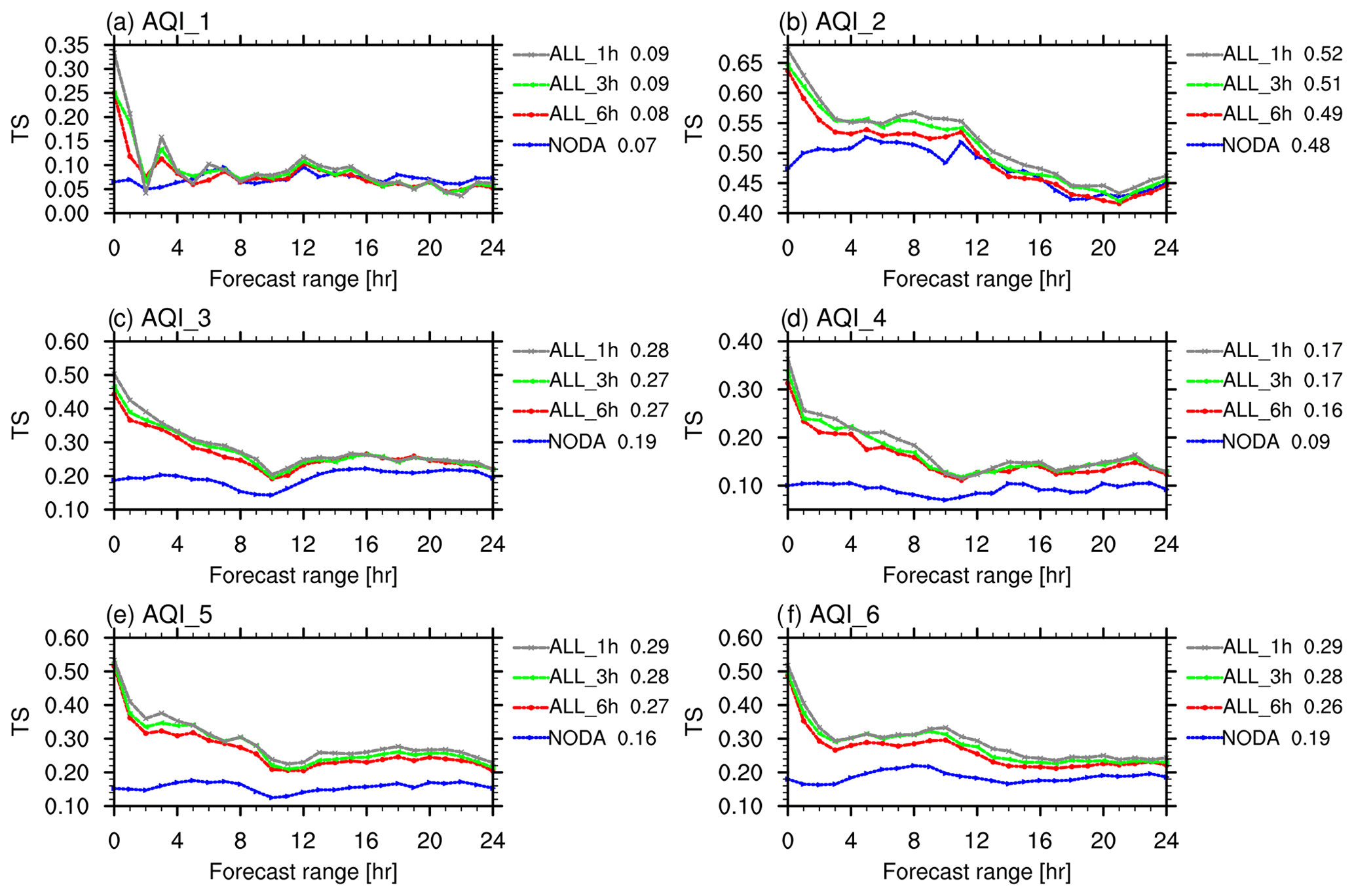
Figure 12Same as Fig. 8, but for the experiments NODA, ALL_6h, ALL-3h, and ALL_1h, respectively.
Figure 9 shows the domain-averaged bias and RMSE of the analysis as in Fig. 3, but for experiments with different DA frequencies (ALL_6h, ALL_3h, and ALL_1h; the ALL_6h is the ALL experiment in Table 2). Except for O3, most of the variables display a gradual improvement with the increase in cycling frequency. For example, from the NODA run to the 6 h cycling experiment and then to the 3 and 1 h cycling experiment, the bias (RMSE) for PM2.5 gradually decreases from 36.60 µg m−3 (70.41 µg m−3) to 5.98 µg m−3 (23.15 µg m−3) and then to 5.41 µg m−3 (21.32 µg m−3) and 4.30 µg m−3 (18.54 µg m−3). Similar results also exist for the bias for SO2, NO2, and CO, as well as for the RMSE for PM10, SO2, and CO. In accordance with the gradual improvements in the analyses, the forecast skills increase with the cycling frequency in most of the variables except for O3 (Figs. 10–11). Especially for the forecasts of aerosols, evident gradual improvements can be seen from 0 to 24 h. From the 6 h cycling experiment to the 3 and 1 h cycling experiment, the averaged decrease percentage of RMSE for PM2.5 (PM10) enlarges from 38.76 % to 41.27 % and 44.21 % (27.31 % to 30.17 % and 32.97 %); the average increased percentage of correlation for PM2.5 (PM10) enlarges from 42.82 % to 49.51 % and 55.58 % (57.71 % to 66.39 % and 74.89 %). To further investigate the integrated DA effect of aerosols and gas-phase pollutants under a different cycling frequency, the TS for AQI is shown in Fig. 12. The forecast of air quality is improved step by step with the increase in cycling frequency. On AQI levels 2–6, the TS for the ALL_1h experiment is situated above the ALL_3h experiment most of the time and is followed by the ALL_6h experiment. These results indicate that frequent IC updating is helpful to further improve the forecast for most of the pollutants.
However, the analysis and 24 h forecast of O3 become worse under higher cycling frequencies for this winter season (Figs. 9e and 11c). Given that the analysis is at 00:00 UTC, the worsening of the analysis in the experiments with higher DA frequencies (1 h, 3 h) could be mainly due to the unfavorable changes in the 1 h and 3 h forecasts period (starting from 23:00 and 21:00 UTC), which is different from the situation in the 6 h cycling experiment. As for the forecasts, the 24 h performances starting from 00:00 UTC show complex changes along with the forecast range: compared to the 6 h cycling experiment, the biases in the experiments with higher DA frequencies decrease at 09:00–14:00 UTC but increase for other hours. The RMSE and correlations in the experiments with higher DA frequencies become worse at most of the hours (Fig. 11c). It should be mentioned that O3 is a relatively short-lived chemical reactive species and takes part in highly complex and photochemical reactions in association with NOx and volatile organic compounds (VOCs) (Peng et al., 2018; Lu et al., 2019). From this perspective, the performances of O3 could also rely on the photochemistry and the NOx titration, in addition to the IC. Although the winter month (January 2017) is investigated here when ozone photochemistry is relatively weak compared to other seasons, the photochemistry and the NOx titration still play their roles. Accordingly, when the assimilation of NO2 changes the NO2 concentration and leaves the NO and VOC unadjusted due to the absence of NO and VOC measurements, two results might occur: firstly, the NO2 ∕ VOC ratio, which determines the photochemical reactions, and even the regime might be changed (O3 production or loss direction might change); secondly, the NOx titration process might be changed due to the NO2 concentration updates (but no change in NO). Considering that the relevant NOx–VOC–O3 reactions take place quickly, changing the O3 concentration in a short period, the advantage of IC DA could compete with the disadvantages of the disordered photochemistry (inaccurate NO2 ∕ VOC ratios) or the changed titration (adjusted NO2 concentrations but not NO) resulting from the DA. Under these circumstances, the more frequently the O3 and NO2 were assimilated, the more incompatibilities could be brought into the related photochemical or titration reactions, resulting in the model performing worse in the O3 forecasts under higher cycling frequencies. It is noted that these statistics were only for the analysis at 00:00 UTC and the 24 h forecast starting from 00:00 UTC for winter season. Since O3 has strong diurnal and seasonal variations, more experiments and statistics at different times of the day and different seasons of the year should be conducted in the future.
According to the results above, it is better to assimilate PM2.5, PM10, SO2, and CO every 1 h and assimilate O3 and NO2 every 6 h in future applications, given the fact that the 6 h cycling experiment performs the best in the O3 forecasting (Fig. 11c) and displays no significant differences in the NO2 forecasting with experiments under higher cycling frequencies (Fig. 11b). It could also be helpful to assimilate the VOC along with O3 and NO2 after there are corresponding observations.
3.4 Indications on further model development
A higher forecast skill relies not only on a better working of DA but also on a better performance of the forecast model. To further improve the forecast skill, a crucial task is to understand the deficiencies in the model, while the challenge in chemistry model diagnostic is that uncertainties from various aspects are mixed up in the model simulations, and the situation becomes even more complex when the reaction path is not yet revealed by the laboratory. However, with the help of DA, as one aspect (IC) in the model is corrected by using observations as constraints, the deficiencies of other aspects (e.g., chemical reactions) could be more evident, and thus there could be a better chance of diagnosing the deficiencies in the model. Specifically, sulfate–nitrate–ammonium (SNA) are the predominant inorganic aerosol species that contribute up to 50 % of total PM2.5 in heavily polluted events in northern China (Y. Wang et al., 2014). In addition to the normal pathways in the MOSAIC scheme, we added SO2–NO2–NO3-related heterogeneous reactions for the high relative-humidity case in WRF-Chem (Chen et al., 2016), which greatly improved the underestimated SNA simulations. Since the newly added reactions are calculated on both the concentration of precursors (SO2, NO2−NO3) and the uptake coefficients in the model, after DA corrected the concentrations of the precursors (one aspect), the impacts of the uptake coefficients could be more evident (the other aspect, not corrected). Ideally, if the newly added reactions depict the heterogeneous reaction processes properly, a forecast improvement for the aerosols could be expected by assimilating their gaseous precursors. Based on this notion, this section verifies the forecast of two specific aerosol species – sulfate () and nitrate () – against a size-resolved particle observation over Beijing IUM station (in view of the assimilated SO2 and NO2 being the corresponding gaseous precursors of these aerosol species), aiming to explore the deficiencies in the uptake coefficients in the newly added heterogeneous reactions and to provide beneficial indications for future model development.
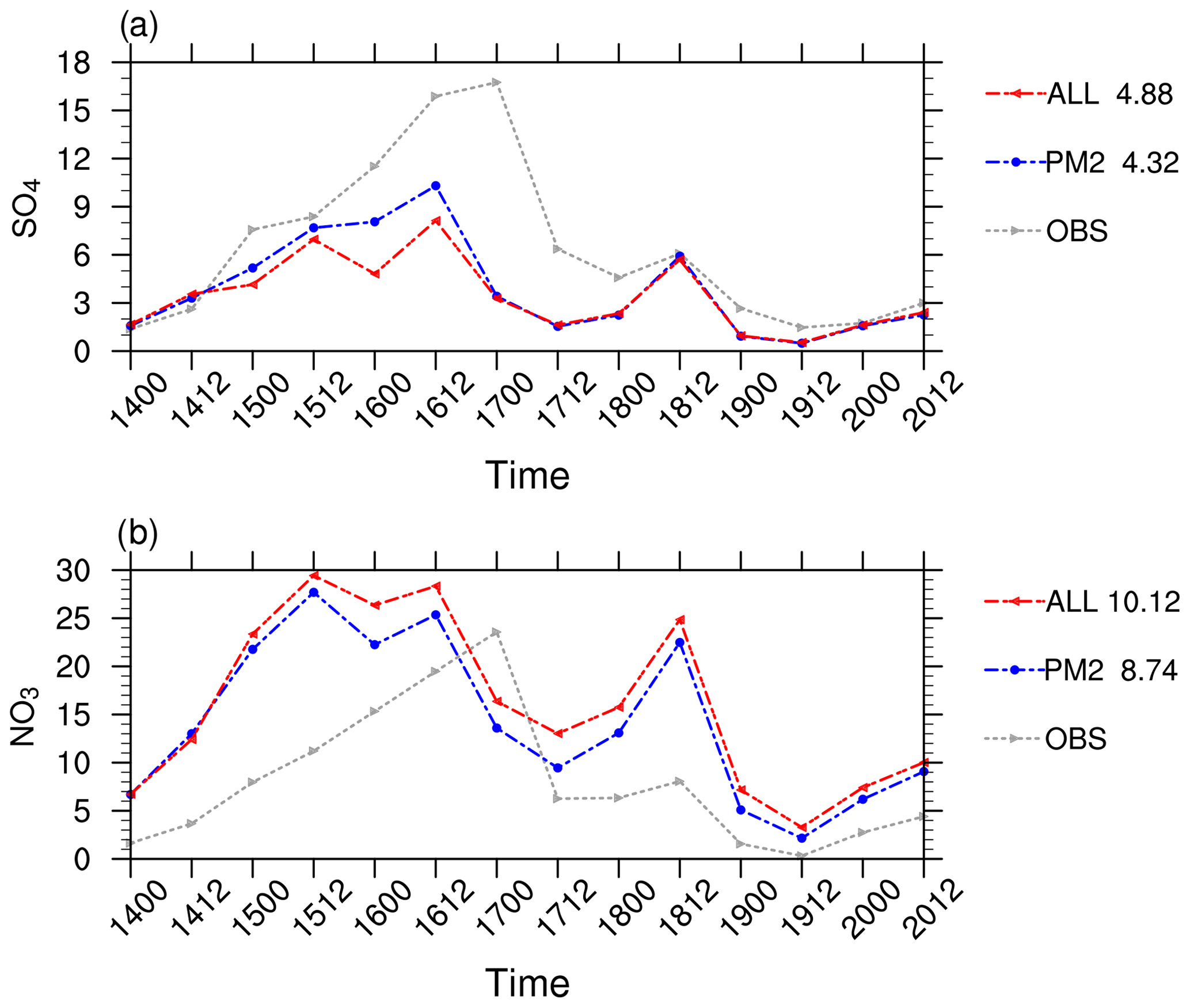
Figure 13Time series of (a) sulfate and (b) nitrate over 14–20 January, verified against the size-resolved particle observation at IUM station (units: µg m−3). The gray, blue, and red lines denote the observation and the results of experiments PM2 and ALL, respectively. The numbers to the right of each panel denote the averaged RMSE over 14–20 January for different experiments.
Figure 13 presents the time series of sulfate and nitrate over Beijing IUM station. In the ALL experiment, after assimilating both the PM concentrations and the gaseous precursors (SO2, NO2), the forecasts of sulfate and nitrate become even worse than the PM2 experiment, which only assimilates the PM concentrations. In the ALL experiment, sulfate experiences a decrease, accompanied by the average RMSE grows from 4.32 to 4.88 µg m−3; nitrate shows an increase, accompanied by the average RMSE grows from 8.74 to 10.12 µg m−3. However, compared to the PM2 experiment, the precursors (SO2 and NO2) are indeed improved. Figure 14 displays the analysis statistics of SO2 and NO2 in the ALL experiment around the Beijing area (red dots in Fig. 1) on 16 January, the period with the largest changes of sulfate and nitrate (Fig. 13). To correct the overestimated SO2 (underestimated NO2) in the background, the DA reduces (enhances) the model value in the ALL experiment, making it closer to the observations.
It should be mentioned that the heterogeneous reactions are added by using the sulfate–nitrate–ammonium observations as constraints to tune the “observation-best-matched” uptake coefficients under the scenario without DA, in which the precursor concentrations are from a pure model and thus not very accurate. To best match the observation, when gaseous precursors are overestimated (underestimated) in the model, the uptake coefficient is tuned to a low-biased (high-biased) value. As a result, such a coefficient may no longer be suited for the cases with DA. For instance, after DA reduces the overestimated SO2, the uptake coefficient is still relatively low and thus the reaction from SO2 to sulfate will stay at a low rate (with both a low value of SO2 and a low reaction coefficient). A similar result also exists for the reaction from NO2 to nitrate. From this perspective, the negative effects on sulfate and nitrate in the ALL experiment may not be hard to understand (Fig. 13). Therefore, in future chemistry development, it is necessary to develop more appropriate coefficients for different gaseous precursor scenarios, in which more constraints, such as precursor and species concentrations, should be provided with the help of the DA technique. Accordingly, further improvements for aerosol forecast could be expected by assimilating their gaseous precursors.
According to the results above, the DA technique provides an opportunity to identify and diagnose the deficiencies in the model. By correcting the precursor concentrations through DA (one aspect), the deficiency of the uptake coefficients for the SNA heterogeneous reactions (the other aspect, not corrected) is revealed. In the future, besides being used to improve the forecast skill through updating the IC, DA could be used as another approach to reveal the necessary developments in the model.
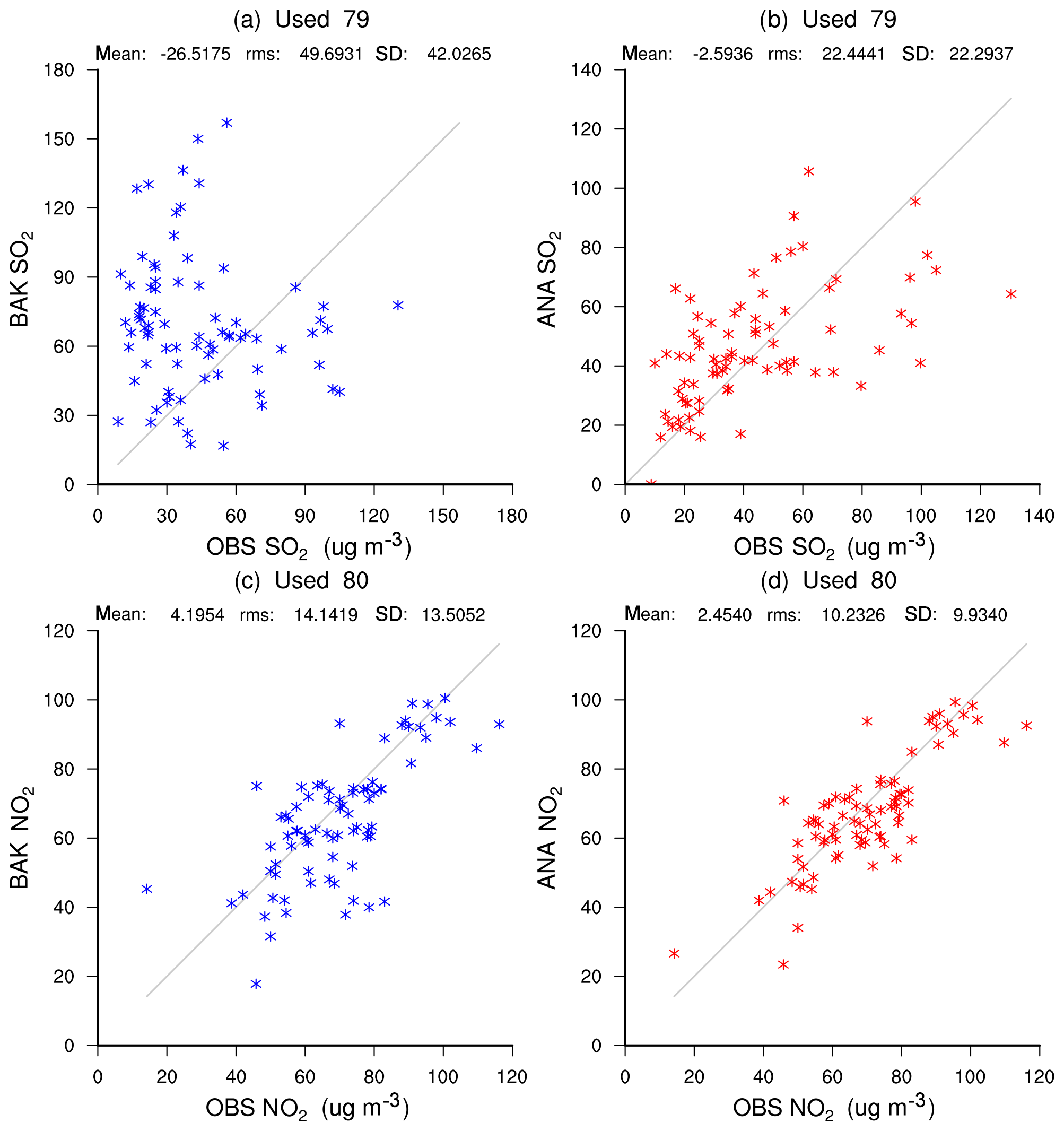
Figure 14Averaged scatterplot of (a, c) observation versus background and (b, d) observation versus analysis for (a, b) SO2 and (c, d) NO2 around the Beijing area (red dots in Fig. 1) on 16 January. The numbers above the panels denote the accumulated numbers of the observations used around the Beijing area on 16 January (16:00, 16:06, 16:12, and 16:18 UTC).
To improve the operational air quality forecasting over China, a flexible aerosol and gas-phase pollutants assimilation capability that can switch between different aerosol schemes is developed based on the WRFDA system with the 3DVAR algorithm. This flexibility is designed to address the complexity of current aerosol schemes and to facilitate future chemistry developments. In this first application, the assimilation capability of surface observations of six major pollutants, including PM2.5, PM10, SO2, NO2, O3, and CO, is built with the MOSAIC aerosol scheme.
Before application in the operational air quality model, capability of the WRFDA-Chem system is verified in terms of analysis and forecast performances. Using the updated system, five DA experiments (assimilating different combinations of pollutants in various frequencies) were conducted for January 2017, along with a control experiment without DA. Results show that the WRFDA-Chem system evidently improves the forecast of aerosols and gas-phase pollutants. From the aspect of analysis, the assimilation of different atmospheric-composition observation reduces the bias and RMSE in the IC remarkably (i.e., by about 68 %, 61 %, and 30 %–60 % in the RMSE for PM2.5, PM10, and gas-phase pollutants); from the aspect of forecast skill, better performances are acquired up to 24 h with about 10 %–40 % (30 %–50 %) improvements in the RMSE (correlation) for different pollutants. Among the different experiments, the one assimilating all the six pollutants displays the best forecast error statistics for most of the pollutants, along with the highest TS for AQI. In future applications, to obtain a better analysis and forecast skill in general, it is recommended to assimilate the six major pollutants simultaneously.
As the cycling frequency is an important aspect in the DA strategy, DA experiments with various cycling frequencies are also analyzed. Results show that the responses toward IC updating are different among the pollutants. For PM2.5, PM10, SO2, and CO, the forecast skills increase with the DA frequency; for O3, compared to a better performance at the 6 h cycling frequency, its analysis at 00:00 UTC and the following 24 h forecast become generally worse under higher cycling frequencies for this winter season, although the biases did decrease at 09:00–14:00 UTC in the 24 h forecast. Considering that the relevant NOx–VOC–O3 reaction system changes the NO2 ∕ O3 concentration in a short period, the advantage of IC DA could compete with the disadvantages of the disordered photochemistry (inaccurate NO2 ∕ VOC ratios) or the changed titration (adjusted NO2 concentrations but not NO) resulting from the DA. In future applications, it is better to assimilate PM2.5, PM10, SO2, and CO every 1 h. For the frequency of O3 and NO2 assimilation, every 6 h is the best in this winter season in our study. Since O3 has strong diurnal and seasonal variations, more experiments and statistics at different times of the day and different seasons of the year should be conducted in the future. Also, it might be helpful to assimilate NO ∕ VOC simultaneously with O3 and NO2 after there are corresponding measurements.
By investigating the effect of assimilating gaseous precursors on the forecast of related aerosols, the deficiencies in the WRF-Chem model are further revealed. The uptake coefficients for sulfate–nitrate–ammonium heterogeneous reactions in the model are found to be not appropriate in the applications with gaseous precursor (SO2 and NO2) assimilations, since they were originally tuned under the gaseous precursor scenarios without DA and the biases from the two aspects (SNA reactions and IC DA) were just compensated. In future chemistry development, it is necessary to develop appropriate coefficients for different gaseous precursor scenarios, in which more constraints, such as precursor and species concentrations, should be provided with the help of the DA technique.
As for the significantly underestimated PMcoarse in the model, the results might relate to the missing emissions under current situations. Different from the United States or European countries, where national emission inventories are provided and updated frequently by the government (e.g., the US National Emission Inventory NEI 05-08-11-14-17), the publicly available emission inventories for China are mainly established by several scientific research groups. As a result, the uncertainties of the publicly available emission inventories in China are relatively large compared with others (US, European countries), and it is a known problem that the fugitive dust emissions over the whole of China is still lacking, which might cause the underestimated PMcoarse simulation in the model.
Due to the flexible aerosol assimilation capability of the WRFDA-Chem system, the development of other aerosol schemes targeting different regions in Asia is underway. In the next step, a study will focus on assimilating chemical observations from different observing platforms, such as satellite aerosol optical depth (AOD) observations, which contain more information over the areas with sparse surface observations. In addition, more advanced DA techniques, such as 4DVAR and Hybrid DA, could be taken into consideration in further developing the aerosol or chemical DA system.
The data used in the figures and the developed WRFDA-Chem codes are available from Wei Sun upon request.
The supplement related to this article is available online at: https://doi.org/10.5194/acp-20-9311-2020-supplement.
WS and ZL conducted the development of the DA system. ZL, DC, WS, and MC designed the research; WS performed experiments and analyzed results; PZ provided PM species observations, and WS and DC wrote the paper with contributions from all co-authors.
The authors declare that they have no conflict of interest.
This work was supported by the National Key R&D Program on Monitoring, Early Warning and Prevention of Major Natural Disasters under grant no. 2017YFC1501406, and the Basic R&D special fund for central-level, scientific research institutes (IUMKYSZHJ201701, IUMKY201807) of China. NCAR is sponsored by the US National Science Foundation.
This research has been supported by the National Key R&D Program on Monitoring, Early Warning and Prevention of Major Natural Disasters (grant no. 2017YFC1501406) and the Basic R&D special fund for central-level, scientific research institutes of China (grant no. IUMKYSZHJ201701, IUMKY201807).
This paper was edited by Chul Han Song and reviewed by two anonymous referees.
Bannister, R.: A review of operational methods of variational and ensemble-variational data assimilation, Q. J. Roy. Meteor. Soc., 143, 607–633, 2017.
Chen, D., Liu, Z., Fast, J., and Ban, J.: Simulations of sulfate–nitrat–ammonium (SNA) aerosols during the extreme haze events over northern China in October 2014, Atmos. Chem. Phys., 16, 10707–10724, https://doi.org/10.5194/acp-16-10707-2016, 2016.
Chen, D., Liu, Z., Ban, J., Zhao, P., and Chen, M.: Retrospective analysis of 2015–2017 wintertime PM2.5 in China: response to emission regulations and the role of meteorology, Atmos. Chem. Phys., 19, 7409–7427, https://doi.org/10.5194/acp-19-7409-2019, 2019.
Chen, F. and Dudhia, J.: Coupling an advanced land surface–hydrology model with the Penn State–NCAR MM5 modeling system. Part I: Model implementation and sensitivity, Mon. Weather Rev., 129, 569–585, 2001.
Chou, M.-D. and Suarez, M. J.: An efficient thermal infrared radiation parameterization for use in general circulation models, NASA Tech. Memo, TM 104606, 3, 25 pp., NASA Goddard Space Flight Cent., Greenbelt, MD, USA, 1994.
Descombes, G., Auligné, T., Vandenberghe, F., Barker, D. M., and Barré, J.: Generalized background error covariance matrix model (GEN_BE v2.0), Geosci. Model Dev., 8, 669–696, https://doi.org/10.5194/gmd-8-669-2015, 2015.
Fan, S., Lu, B., Zhong, J., Wang, Z., Gao, H., Li, Y., He, J., Zhang, W., Zhang, X., Liang, X., Introduction of Rapid-refresh Multi-scale Analysis and Prediction System-short time (RMAP-ST) over Northern China, 33th Annual Meeting of Chinese Meteorological Society, Xi'an, China, 2016 (in Chinese).
Fast, J. D., Gustafson, W. I., Easter, R. C., Zaveri, R. A., Barnard, J. C., Chapman, E. G., Grell, G. A., and Peckham, S. E.: Evolution of ozone, particulates, and aerosol direct radiative forcing in the vicinity of Houston using a fully coupled meteorology-chemistry-aerosol model, J. Geophys. Res.-Atmos., 111, D21305, https://doi.org/10.1029/2005jd006721, 2006.
Fu, Y., Liao, H., and Yang, Y.: Interannual and decadal changes in tropospheric ozone in China and the associated chemistry-climate interactions: A review, Adv. Atmos. Sci., 36, 975–993, 2019.
Grell, G. A. and Dévényi, D.: A generalized approach to parameterizing convection combining ensemble and data assimilation techniques, Geophys. Res. Lett., 29, 1693, https://doi.org/10.1029/2002gl015311, 2002.
Grell, G. A., Peckham, S. E., Schmitz, R., McKeen, S. A., Frost, G., Skamarock, W. C., and Eder, B.: Fully coupled “online” chemistry within the WRF model, Atmos. Environ., 39, 6957–6975, 2005.
He, K.: Multi-resolution emission Inventory for China (MEIC): model framework and 1990–2010 anthropogenic emissions, International Global Atmospheric Chemistry Conference, Beijing, China, 17–21 September 2012, 2012AGUFM.A32B..05H, 2012.
Hong, S.-Y., Noh, Y., and Dudhia, J.: A new vertical diffusion package with an explicit treatment of entrainment processes, Mon. Weather Rev., 134, 2318–2341, 2006.
Huang, X., Song, Y., Zhao, C., Li, M., Zhu, T., Zhang, Q., and Zhang, X.: Pathways of sulfate enhancement by natural and anthropogenic mineral aerosols in China, J. Geophys. Res.-Atmos., 119, 14165–114179, 2014.
Jiang, Z., Liu, Z., Wang, T., Schwartz, C. S., Lin, H. C., and Jiang, F.: Probing into the impact of 3DVAR assimilation of surface PM10 observations over China using process analysis, J. Geophys. Res.-Atmos., 118, 6738–6749, 2013.
Kumar, A. and Goyal, P.: Forecasting of daily air quality index in Delhi, Sci. Total environ., 409, 5517–5523, 2011.
Lei, Y., Zhang, Q., He, K. B., and Streets, D. G.: Primary anthropogenic aerosol emission trends for China, 1990–2005, Atmos. Chem. Phys., 11, 931–954, https://doi.org/10.5194/acp-11-931-2011, 2011.
Li, M., Zhang, Q., Streets, D. G., He, K. B., Cheng, Y. F., Emmons, L. K., Huo, H., Kang, S. C., Lu, Z., Shao, M., Su, H., Yu, X., and Zhang, Y.: Mapping Asian anthropogenic emissions of non-methane volatile organic compounds to multiple chemical mechanisms, Atmos. Chem. Phys., 14, 5617–5638, https://doi.org/10.5194/acp-14-5617-2014, 2014.
Liu, Z. Q., Liu, Q. H., Lin, H. C., Schwartz, C. S., Lee, Y. H., and Wang, T. J.: Three-dimensional variational assimilation of MODIS aerosol optical depth: Implementation and application to a dust storm over East Asia, J. Geophys. Res.-Atmos., 116, D23206, https://doi.org/10.1029/2011jd016159, 2011.
Lu, X., Zhang, L., Chen, Y., Zhou, M., Zheng, B., Li, K., Liu, Y., Lin, J., Fu, T.-M., and Zhang, Q.: Exploring 2016–2017 surface ozone pollution over China: source contributions and meteorological influences, Atmos. Chem. Phys., 19, 8339–8361, https://doi.org/10.5194/acp-19-8339-2019, 2019.
McHenry, J. N., Vukovich, J. M., and Hsu, N. C.: Development and implementation of a remote-sensing and in situ data-assimilating version of CMAQ for operational PM2.5 forecasting. Part 1: MODIS aerosol optical depth (AOD) data-assimilation design and testing, Japca. J. Air Waste Ma., 65, 1395–1412, 2015.
McKeen, S., Grell, G., Peckham, S., Wilczak, J., Djalalova, I., Hsie, E. Y., Frost, G., Peischl, J., Schwarz, J., Spackman, R., Holloway, J., de Gouw, J., Warneke, C., Gong, W., Bouchet, V., Gaudreault, S., Racine, J., McHenry, J., McQueen, J., Lee, P., Tang, Y., Carmichael, G. R., and Mathur, R.: An evaluation of real-time air quality forecasts and their urban emissions over eastern Texas during the summer of 2006 Second Texas Air Quality Study field study, J. Geophys. Res.-Atmos., 114, D00F11, https://doi.org/10.1029/2008jd011697, 2009.
Mlawer, E. J., Taubman, S. J., Brown, P. D., Iacono, M. J., and Clough, S. A.: Radiative transfer for inhomogeneous atmospheres: RRTM, a validated correlated-k model for the longwave, J. Geophys. Res.-Atmos., 102, 16663–16682, 1997.
Nie, W., Ding, A. J., Wang, T., Kerminen, V. M., George, C., Xue, L. K., Wang, W. X., Zhang, Q. Z., Petaja, T., Qi, X. M., Gao, X. M., Wang, X. F., Yang, X. Q., Fu, C. B., and Kulmala, M.: Polluted dust promotes new particle formation and growth, Sci. Rep.-UK, 4, 6634 https://doi.org/10.1038/srep06634, 2014.
Pang, J., Liu, Z., Wang, X., Bresch, J., Ban, J., Chen, D., and Kim, J.: Assimilating AOD retrievals from GOCI and VIIRS to forecast surface PM2.5 episodes over Eastern China, Atmos. Environ., 179, 288–304, 2018.
Parrish, D. F. and Derber, J. C.: The National-Meteorological-Centers Spectral Statistical-Interpolation Analysis System, Mon. Weather Rev., 120, 1747–1763, https://doi.org/10.1175/1520-0493(1992)120<1747:Tnmcss>2.0.Co;2, 1992.
Peng, Z., Liu, Z., Chen, D., and Ban, J.: Improving PM2.5 forecast over China by the joint adjustment of initial conditions and source emissions with an ensemble Kalman filter, Atmos. Chem. Phys., 17, 4837–4855, https://doi.org/10.5194/acp-17-4837-2017, 2017.
Peng, Z., Lei, L., Liu, Z., Sun, J., Ding, A., Ban, J., Chen, D., Kou, X., and Chu, K.: The impact of multi-species surface chemical observation assimilation on air quality forecasts in China, Atmos. Chem. Phys., 18, 17387–17404, https://doi.org/10.5194/acp-18-17387-2018, 2018.
Sandu, A. and Chai, T.: Chemical data assimilation – An overview, Atmosphere-Basel, 2, 426–463, 2011.
Schutgens, N. A. J., Miyoshi, T., Takemura, T., and Nakajima, T.: Applying an ensemble Kalman filter to the assimilation of AERONET observations in a global aerosol transport model, Atmos. Chem. Phys., 10, 2561–2576, https://doi.org/10.5194/acp-10-2561-2010, 2010.
Schwartz, C. S., Liu, Z., Lin, H. C., and McKeen, S. A.: Simultaneous three-dimensional variational assimilation of surface fine particulate matter and MODIS aerosol optical depth, J. Geophys. Res.-Atmos., 117, D13202, https://doi.org/10.1029/2011JD017383, 2012.
Sekiyama, T. T., Tanaka, T. Y., Shimizu, A., and Miyoshi, T.: Data assimilation of CALIPSO aerosol observations, Atmos. Chem. Phys., 10, 39–49, https://doi.org/10.5194/acp-10-39-2010, 2010.
Su, J., Zhao, P., and Dong, Q.: Chemical compositions and liquid water content of size-resolved aerosol in Beijing, Aerosol Air Qual. Res., 18, 680–692, 2018.
Tang, X., Zhu, J., Wang, Z. F., and Gbaguidi, A.: Improvement of ozone forecast over Beijing based on ensemble Kalman filter with simultaneous adjustment of initial conditions and emissions, Atmos. Chem. Phys., 11, 12901–12916, https://doi.org/10.5194/acp-11-12901-2011, 2011.
Tang, X., Zhu, J., Wang, Z. F., Wang, M., Gbaguidi, A., Li, J., Shao, M., Tang, G. Q., and Ji, D. S.: Inversion of CO emissions over Beijing and its surrounding areas with ensemble Kalman filter, Atmos. Environ., 81, 676–686, https://doi.org/10.1016/j.atmosenv.2013.08.051, 2013.
Tao, J., Zhang, L., Gao, J., Wang, H., Chai, F., and Wang, S.: Aerosol chemical composition and light scattering during a winter season in Beijing, Atmos. Environ., 110, 36–44, 2015.
Wang, G., Zhang, R., Gomez, M. E., Yang, L., Levy Zamora, M., Hu, M., Lin, Y., Peng, J., Guo, S., Meng, J., Li, J., Cheng, C., Hu, T., Ren, Y., Wang, Y., Gao, J., Cao, J., An, Z., Zhou, W., Li, G., Wang, J., Tian, P., Marrero-Ortiz, W., Secrest, J., Du, Z., Zheng, J., Shang, D., Zeng, L., Shao, M., Wang, W., Huang, Y., Wang, Y., Zhu, Y., Li, Y., Hu, J., Pan, B., Cai, L., Cheng, Y., Ji, Y., Zhang, F., Rosenfeld, D., Liss, P. S., Duce, R. A., Kolb, C. E., and Molina, M. J.: Persistent sulfate formation from London Fog to Chinese haze, P. Natl. Acad. Sci. USA, 113, 13630–13635, https://doi.org/10.1073/pnas.1616540113, 2016.
Wang, L. T., Wei, Z., Yang, J., Zhang, Y., Zhang, F. F., Su, J., Meng, C. C., and Zhang, Q.: The 2013 severe haze over southern Hebei, China: model evaluation, source apportionment, and policy implications, Atmos. Chem. Phys., 14, 3151–3173, https://doi.org/10.5194/acp-14-3151-2014, 2014.
Wang, Y. X., Zhang, Q. Q., Jiang, J. K., Zhou, W., Wang, B. Y., He, K. B., Duan, F. K., Zhang, Q., Philip, S., and Xie, Y. Y.: Enhanced sulfate formation during China's severe winter haze episode in January 2013 missing from current models, J. Geophys. Res.-Atmos., 119, 10425–10440 https://doi.org/10.1002/2013jd021426, 2014.
Wild, O., Zhu, X., and Prather, M. J.: Fast-J: Accurate simulation of in-and below-cloud photolysis in tropospheric chemical models, J. Atmos. Chem., 37, 245–282, 2000.
Xie, Y. N., Ding, A. J., Nie, W., Mao, H. T., Qi, X. M., Huang, X., Xu, Z., Kerminen, V. M., Petaja, T., Chi, X. G., Virkkula, A., Boy, M., Xue, L. K., Guo, J., Sun, J. N., Yang, X. Q., Kulmala, M., and Fu, C. B.: Enhanced sulfate formation by nitrogen dioxide: Implications from in situ observations at the SORPES station, J. Geophys. Res.-Atmos., 120, 12679–12694, https://doi.org/10.1002/2015jd023607, 2015.
Yu, M., Miao, S., and Zhang, H.: Uncertainties in the Impact of Urbanization on Heavy Rainfall: Case Study of a Rainfall Event in Beijing on 7 August 2015, J. Geophys. Res.-Atmos., 123, 6005–6021, 2018.
Zaveri, R. A. and Peters, L. K.: A new lumped structure photochemical mechanism for large-scale applications, J. Geophys. Res.-Atmos., 104, 30387–30415, 1999.
Zaveri, R. A., Easter, R. C., Fast, J. D., and Peters, L. K.: Model for Simulating Aerosol Interactions and Chemistry (MOSAIC), J. Geophys. Res.-Atmos., 113, D13204, https://doi.org/10.1029/2007jd008782, 2008.
Zhang, Q., Streets, D. G., Carmichael, G. R., He, K. B., Huo, H., Kannari, A., Klimont, Z., Park, I. S., Reddy, S., Fu, J. S., Chen, D., Duan, L., Lei, Y., Wang, L. T., and Yao, Z. L.: Asian emissions in 2006 for the NASA INTEX-B mission, Atmos. Chem. Phys., 9, 5131–5153, https://doi.org/10.5194/acp-9-5131-2009, 2009.
Zheng, S., Cao, C.-X., and Singh, R. P.: Comparison of ground based indices (API and AQI) with satellite based aerosol products, Sci. Total environ., 488, 398–412, 2014.
Zheng, B., Zhang, Q., Zhang, Y., He, K. B., Wang, K., Zheng, G. J., Duan, F. K., Ma, Y. L., and Kimoto, T.: Heterogeneous chemistry: a mechanism missing in current models to explain secondary inorganic aerosol formation during the January 2013 haze episode in North China, Atmos. Chem. Phys., 15, 2031–2049, https://doi.org/10.5194/acp-15-2031-2015, 2015.