the Creative Commons Attribution 4.0 License.
the Creative Commons Attribution 4.0 License.
 | 24 Jul 2020
A convolution of observational and model data to estimate age of air spectra in the northern hemispheric lower stratosphere
Marius Hauck
Harald Bönisch
Peter Hoor
Timo Keber
Felix Ploeger
Tanja J. Schuck
Andreas Engel
Derivation of mean age of air (AoA) and age spectra from atmospheric measurements remains a challenge and often requires output from atmospheric models. This study tries to minimize the direct influence of model output and presents an extension and application of a previously established inversion method to derive age spectra from mixing ratios of long- and short-lived trace gases. For a precise description of cross-tropopause transport processes, the inverse method is extended to incorporate air entrainment into the stratosphere across the tropical and extratropical tropopause. We first use simulations with the Chemical Lagrangian Model of the Stratosphere (CLaMS) to provide a general proof of concept of the extended principle in a controllable and consistent environment, where the method is applied to an idealized set of 10 trace gases with predefined constant lifetimes and compared to reference model age spectra. In the second part of the study we apply the extended inverse method to atmospheric measurements of multiple long- and short-lived trace gases measured aboard the High Altitude and Long Range (HALO) research aircraft during the two research campaigns POLSTRACC–GW-LCYCLE–SALSA (PGS) and Wave-driven Isentropic Exchange (WISE). As some of the observed species undergo significant loss processes in the stratosphere, a Monte Carlo simulation is introduced to retrieve age spectra and chemical lifetimes in stepwise fashion and to account for the large uncertainties. Results show that in the idealized model scenario the inverse method retrieves age spectra robustly on annual and seasonal scales. The extension to multiple entry regions proves reasonable as our CLaMS simulations reveal that in the model between 50 % and 70 % of air in the lowermost stratosphere has entered through the extratropical tropopause (30–90∘ N and S) on annual average. When applied to observational data of PGS and WISE, the method derives age spectra and mean AoA with meaningful spatial distributions and quantitative range, yet large uncertainties. Results indicate that entrainment of fresh tropospheric air across both the extratropical and tropical tropopause peaked prior to both campaigns, but with lower mean AoA for WISE than PGS data. The ratio of moments for all retrieved age spectra for PGS and WISE is found to range between 0.52 and 2.81 years. We conclude that the method derives reasonable and consistent age spectra using observations of chemically active trace gases. Our findings might contribute to an improved assessment of transport with age spectra in future studies.
- Article
(4335 KB) - Full-text XML
-
Supplement
(509 KB) - BibTeX
- EndNote


Spatial distributions of many greenhouse gases and ozone-depleting trace gases throughout the stratosphere are determined by the global mean meridional circulation, known as the Brewer–Dobson circulation (BDC), making it a crucial factor for the Earth's radiative budget and climate (Shepherd, 2007; Solomon et al., 2010). The BDC is usually characterized as a superposition of a mean residual circulation with net mass transport and two-way eddy mixing with tracer exchange but no net mass flux (Plumb, 2002; Butchart, 2014). Birner and Bönisch (2011) recognized two distinct pathways for the BDC, a shallow and a deep branch, with different transport timescales along them. The shallow branch reaches from the tropics into the extratropics close to the tropopause, while the deep branch extends up into the middle and upper stratosphere (Birner and Bönisch, 2011). Mechanical drivers of the BDC are planetary- and synoptic-scale atmospheric waves that get excited in the troposphere and propagate upward into the extratropical middle stratosphere where they finally break and transfer their momentum to induce a poleward motion (Haynes et al., 1991; Holton et al., 1995). The wave drag causes air to rise slowly in the tropics mainly through the tropical tropopause layer (TTL) to compensate for the poleward drift (Fueglistaler et al., 2009). Eventually, air descends at higher latitudes back into the troposphere. The upward mass flux in the tropics presents a distinct seasonality with maximum upward transport during northern hemispheric winter, due to a maximum of tropospheric waves (Rosenlof and Holton, 1993; Rosenlof, 1995). Although the TTL is identified as the main entry point to the stratosphere, transport mechanisms across the extratropical tropopause play an important role in air composition in the lowermost stratosphere (LMS) below 380 K potential temperature (Olsen et al., 2004; Boothe and Homeyer, 2017). Those exchange processes exhibit their own distinct seasonality (Appenzeller et al., 1996; Schoeberl, 2004) and geographical distribution (Škerlak et al., 2014; Yang et al., 2016).
As global greenhouse gas concentrations and sea surface temperatures keep rising, model studies expect that the BDC will strengthen due to enhanced wave drag (Garcia and Randel, 2008; Li et al., 2008; Shepherd and McLandress, 2011). Studies of suitable dynamical tracers (e.g., SF6, CO2 or N2O) from different observational sources, however, show a much more complex and contradictory state, indicating that the strength of the BDC might undergo nonuniform structural changes with hemispheric asymmetries (Engel et al., 2009; Bönisch et al., 2011; Ray et al., 2014; Stiller et al., 2017; Laube et al., 2020). Although more recent analyses of global models (Oberländer-Hayn et al., 2015, 2016) and also reanalyses (Diallo et al., 2012; Abalos et al., 2015) were able to disentangle some inconsistencies, possible trends of the BDC remain an open issue, especially in the case of reanalyses, as recent studies show that different reanalysis products can alter the outcome significantly (Chabrillat et al., 2018; Ploeger et al., 2019).
A major problem that studies of the BDC share is the difficulty to measure transport directly (Butchart, 2014). While model simulations provide possibilities to derive quantities that describe the strength and structure of the BDC and potential trends, observational analysis is challenging, especially in remote parts of the stratosphere where only sparse measurements exist. A well-established diagnostic tool used in many studies of both models and observations is mean age of air (AoA) (Hall and Plumb, 1994). Mean AoA is defined as the average transit time an air parcel needs to reach the considered location starting at a specified reference surface, usually the Earth's surface or the tropical tropopause. It is inversely proportional to the general circulation strength (Austin and Li, 2006). Mean AoA is also influenced by mixing processes (Waugh and Hall, 2002; Garny et al., 2014), and separation between residual transport and mixing is complicated due to the average nature of mean AoA. For such analysis, a full transit time distribution should be considered, since stratospheric air consists of an irreversible mixture of air parcels with different transit times from the source region. The age spectrum of any arbitrary air parcel represents a probability density function (PDF) of the transit timescales within the parcel (Kida, 1983).
In many model simulations, the age spectrum is constructed by an implementation of chemically inert trace gases that are periodically pulsed in a specified boundary region (Haine et al., 2008; Li et al., 2012; Ploeger and Birner, 2016). Mean AoA is then defined as the first moment of the age spectrum. In the case of observations, the derivation of both mean AoA and age spectra is more complex and follows different approaches. The basis of many past studies has been measurements of (very) long-lived trace gases together with the fundamental theory on age spectra by Hall and Plumb (1994) to constrain the shape of the spectra and the ratio of variance to mean AoA beforehand (Volk et al., 1997; Engel et al., 2002, 2009). Recent results by Fritsch et al. (2019) show that the parameter choice in such constraint methods strongly influences resulting mean AoA trends. Other methods rely on a more general shape of the spectrum but require more data than in the constrained case (Holzer and Primeau, 2010; Holzer and Waugh, 2015). However, the number of suitable stratospheric trace gases with a (very) large chemical lifetime is limited. One possible solution is to additionally consider substances with rapid chemical depletion, since stratospheric chemistry and transport are strongly intertwined. Such approaches also exist in different constrained (Schoeberl et al., 2005; Ehhalt et al., 2007) and unconstrained versions (Schoeberl et al., 2000; Podglajen and Ploeger, 2019). An improved parametric approach has been introduced in Hauck et al. (2019), which relies only on a constrained age spectrum shape to achieve applicability together with well-matched results in a model test scenario. Unfortunately, the method shows quite large discrepancies in the lowermost stratosphere where most stratospheric aircraft measurements are taken.
This paper constitutes a direct follow-up to Hauck et al. (2019). We extend the inverse method described therein to the lowermost stratosphere with a new formulation and provide a short proof of concept using a simulation of the Chemical Lagrangian Model of the Stratosphere (CLaMS) (McKenna, 2002a, b; Pommrich et al., 2014) with idealized radioactive tracers. We then apply the extended method to in situ measurement data gained during the campaigns POLSTRACC–GW-LCYCLE–SALSA (PGS) and Wave-driven Isentropic Exchange (WISE) of the High Altitude and Long Range (HALO) research aircraft and analyze the resulting age spectra and their moments. Section 2 gives insight into the extended formulation of the method and the statistical procedure to estimate age spectra and chemical lifetimes from observations. Section 3 describes the data basis for this study. Finally, results are presented in Sect. 4 and completed by an outlook and a critical discussion in Sect. 5.
2.1 Inverse method – general approach and problems
The theory of the inverse method is provided in detail by Hauck et al. (2019). It is a modified version of the method presented by Schoeberl et al. (2005) and utilizes mixing ratios of a set of different chemically active compounds to derive an age spectrum using a numerical optimization scheme. The age spectrum shape is constrained by the inverse Gaussian distribution proposed by Hall and Plumb (1994). At the same time, seasonality in stratospheric transport, which is visible in modeled age spectra in the form of multiple modes (Reithmeier et al., 2008; Li et al., 2012; Ploeger and Birner, 2016), has to be imposed by a seasonal scaling factor as the inverse Gaussian function is intrinsically a monomodal PDF. Mathematically, the inverse method is based on the following equation.
χ(x,t) denotes the mixing ratio of any arbitrary trace gas at (x,t) in the stratosphere with chemical depletion, but no stratospheric sources. t′ is the transit time through the stratosphere, the mixing ratio time series of the substance at the reference surface, the transit-time-dependent chemical lifetime, the age spectrum, and ω(t′) the seasonal scaling factor to gain multimodal PDFs (see below). n(x,t) is a normalization factor for the age spectrum, which ensures that and have identical norms. It is defined as
The definition of n(x,t) above preserves the norm of the age spectrum during the scaling process. Although age spectra must usually be normalized, there are cases in this study where a non-normalized spectrum is physically meaningful (see Sect. 2.2.1). Full consideration of a transit-time-dependent entry mixing ratio has been introduced for applicability purposes, since many atmospheric trace gases exhibit a strong long-term temporal trend that should be considered properly. An approximation of the stratospheric age spectrum in Eq. (1) is provided by Hall and Plumb (1994):
but with a three-dimensional transport parameter K(x,t) instead of an originally one-dimensional diffusion coefficient. z is the potential temperature difference to the local tropopause and H the scale height of the air density. The first moment Γ(x,t) (i.e., mean AoA) and centered second moment Δ2(x,t) (i.e., variance) of the spectrum are given as (Hall and Plumb, 1994)
For the inversion process, mixing ratios of a given set of distinct trace gases are considered, and K(x,t) is optimized numerically for all species simultaneously. Hauck et al. (2019) provide a general proof of concept of this method in a controllable model environment featuring a set of several artificial radioactive trace gases with constant chemical lifetimes. Despite the robust performance of the inverse method compared to the model reference in general, the lower stratosphere proves challenging, especially during northern hemispheric spring and fall. That is most probably linked to a conceptual flaw in the design of the inverse method. In its presented form, all derived inverse age spectra assume the tropical tropopause to be a single source region into the stratosphere. Although this appears valid for the upper and middle stratosphere (Fueglistaler et al., 2009), studies have shown that for the lowermost extratropical stratosphere, quasi-isentropic transport across the local tropopause has critical influence and strongly affects trace gas burdens in that region (Hoor et al., 2005; Bönisch et al., 2009). Therefore, the assumption of single entry through the tropical tropopause layer is insufficient to estimate a precise age spectrum and must be modified to include air entrainment through the complete tropopause together with related seasonality.
2.2 Inverse method with multiple entry sections
2.2.1 Concept
To fully incorporate transport processes in the extratropical lowermost stratosphere, an extension of the methodology to multiple entry regions is required. A rather intuitive way to divide the tropopause is the partitioning into a northern (index N), a tropical (index T) and a southern (index S) section, each with a separate age spectrum assigned to them. All entry regions must then add up geographically to span the global tropopause. A mathematically strict derivation of age spectra for several different source regions is given by Holzer and Hall (2000). The ansatz is similar to Bönisch et al. (2009), but with a split of the reference surface rather than a separation into a tropospheric and a stratospheric fraction. Due to mass conservation, this concept translates into a composite age spectrum by
with being the age spectrum referring to transport through the tropopause section i. Since the normalization of must also hold in the extended case, the integration of now yields
The lowercased indicates a non-normalized age spectrum and fi(x,t) its respective norm. In terms of transport, the norm fi(x,t) provides an estimate of the fraction of air at (x,t) which has entered the stratosphere through tropopause region i. The norms are referred to as origin fractions and provide an important toolset for an analysis of seasonality in air entrainment (see Sect. 4.1). Any non-normalized age spectrum can be converted into a proper PDF by division through its origin fraction.
Since each constitutes a description of transport for the percentage of air at (x,t) that entered the stratosphere through tropopause region i, it can therefore also be utilized to calculate the mixing ratio fraction χi(x,t) associated with that respective entrainment. Multiplication of Eq. (7) with χ(x,t) includes those mixing ratio fractions in the new concept
where each individual χi(x,t) can be derived from and Eq. (1) as
The parameterization provided by Eq. (3) returns an invariably normalized inverse Gaussian function so that Eq. (10) must be modified with Eq. (8) to correctly yield
Each entry region is now treated with a single entry mixing ratio time series , a transit-time-dependent lifetime τi(t′), a normalized age spectrum , and an imposed seasonal cycle ωi(t′) with its respective normalization factor ni(x,t). The introduced formulation is valid for any partitioning of the tropopause into three subregions. For this study, the tropical tropopause is chosen to range from 30∘ S up to 30∘ N to incorporate the seasonal shift of the intertropical convergence zone (ITCZ). The northern and southern parts extend from 30 to 90∘ N and 30 to 90∘ S, respectively. With that choice, all entry regions span an identical range of 60∘ latitude, although the actual enclosed area is larger for the tropical section. Transport is now characterized by three separate parameters Ki(x,t). Since the mixing ratio fraction χi(x,t) is usually unknown for any stratospheric location, Eq. (11) is divided by fi(x,t) knowing that χi(x,t) has been introduced as . This important step yields a set of three decoupled equations, which can be treated separately:
The inversion process of Eq. (12) is independent of fi(x,t) but only works correctly if or τi(t′) are unequal for all tropopause regions. Otherwise, each inversion leads to the identical age spectrum. Due to refinements of the optimization algorithm, these equations are optimized for all considered species at once now with 0.1 % tolerance (5 % in Hauck et al., 2019) and the new metric of the symmetric signed percentage bias (SSPB) (Morley et al., 2018). The SSPB is suitable if the overall quantitative range of mixing ratios is large and utilizes the median and logarithm to smooth the strong percentage influence of very small mixing ratios. That inversion process is now called K-inversion. Note that the decision to optimize bias rather than variance, e.g., root-mean-square error, has been made to return an average age spectrum that captures even fine effects of the underlying mixing ratio data robustly. In return, this comes at the cost of higher variance around the true solution due to the bias–variance tradeoff.
2.2.2 Extratropical seasonal cycles
Exchange processes across the northern hemispheric (NH) and southern hemispheric (SH) extratropical tropopause each display a different seasonality than the transport through the tropical tropopause layer. These seasonal cycles are relevant for stratospheric age spectra as they cause the multimodal shape of modeled spectra. The inverse method rests upon the monomodal inverse Gaussian function by Hall and Plumb (1994) so that multiple peaks are not included intrinsically but are imposed by the fixed scaling factor ωi(t′) during the inversion process. In Hauck et al. (2019) it has been shown that the ratio of the tropical net upward mass flux at 70 hPa between different seasons can be used to scale the age spectrum at matching transit times. The scaling factor by Hauck et al. (2019) is given as
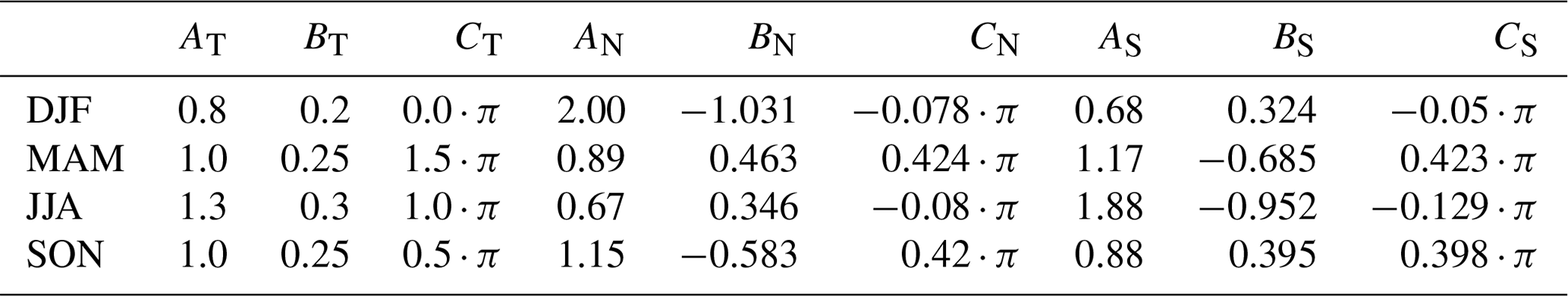
Ai,Bi, and Ci are constants that now depend on the entry region and the considered season. Seasons are hereafter abbreviated as DJF (NH winter), MAM (NH spring), JJA (NH summer), and SON (NH fall). Note that an increase in transit time is always equivalent to going backward in real time so that DJF is followed by SON (0.25 years transit time), JJA (0.5 years), and MAM (0.75 years). The values for the tropical tropopause section are taken from Hauck et al. (2019) and given in the first three columns of Table 1.
Table 1Scaling constants of Eq. (13) for the northern, tropical, and southern tropopause sections (N, T, S) in all four seasons. The tropical values are taken from Hauck et al. (2019).
The extratropical cycles are more challenging as distinct transport processes superimpose in the extratropical lowermost stratosphere. For a proper scaling factor in these regions, a net upward-directed mass flux should be considered that reflects the ongoing dynamical processes as precisely as possible. Previous observationally based studies of SF6, CO2, and mean AoA find a flushing of the NH lowermost stratosphere with fresh tropospheric air during summer (JJA) and autumn (SON) that is most likely linked to the weaker subtropical jet stream and a dominance of the shallow branch of the BDC during that time (Bönisch et al., 2009). In contrast to these results, different mass budget analyses of the lowermost stratosphere in both hemispheres show that the net direction of the hemispherically integrated mass flux across the tropopause is downward with a maximum during spring in each hemisphere and a generally weaker seasonality in the SH. The upward component of this net mass flux is shown to reach its maximum during fall and its minimum conversely in spring in each hemisphere (Olsen et al., 2004; Schoeberl, 2004). The contradicting seasonality patterns imply that a hemispherically integrated mass flux might not be a suitable proxy for upward transport across the defined extratropical tropopause sections in this study, especially since the net direction of this flux is downward. It is more likely that a geographically narrow section of the NH and SH tropopause with year-round net upwelling causes the modes of the age spectra. Yang et al. (2016) investigate the ozone flux across the tropopause with a different framework where regions of net up- and downwelling are distinguishable. Their results indicate that in a small region in the subtropics of each hemisphere (around the equatorward flank of the subtropical jet stream), net upward transport across the tropopause with a maximum in summer is present, while at higher latitudes the net direction of the flux turns downward with a maximum in spring or winter depending on the latitudinal range (see their Fig. 12). In the SH, the seasonality is found to be generally weaker. This matches the observational results for the NH mentioned above. As the subtropical jet region is partly included in the defined tropopause sections for this study (30–90∘ N and S), it is likely that the enhanced entrainment across the subtropical jet stream during summer is a key feature of transport visible in derived age spectra. Unfortunately, Yang et al. (2016) provide only an ozone flux in their study (see their Fig. 7a and b) and no mass flux for the desired region so that a different proxy must be found.
To estimate the seasonality and the strength of the dominant entrainment processes specifically across the introduced extratropical tropopause sections, the modeled age spectra from the CLaMS simulation below are considered, which are initialized in the specified NH and SH tropopause section (see Sect. 3.1 for details on the simulation). We follow the ansatz of Fig. 14b in Ploeger and Birner (2016) and integrate all monthly stratospheric age spectra of one source region bin-wise to compute the fraction of air that entered the stratosphere across this given source region per transit time bin. The fractions of all age spectra are cumulated and transit times are matched correctly against real time so that an average statistic for air mass entrainment across the NH and SH tropopause section per month is retrieved. Results of this ansatz are shown in Fig. 1a, b for the NH (panel a) and SH (panel b) tropopause section. It is evident that in the model for both regions the strongest entrainment occurs during July (NH) and January (SH), where more than 14 % of all air masses that cross the respective tropopause section are found to enter the stratosphere. This seasonality follows the observations of Bönisch et al. (2009) and also the ozone flux of Yang et al. (2016) very well and makes the subtropical jet region the most likely source mechanism for the tropopause sections defined above. The minimum of entrainment is found consistently in December (NH) and June (SH) with a fraction of less than 3 %. The cumulated values for each season are used to derive a scaling factor for the age spectra referring to the NH and SH tropopause sections. For instance, the fraction during JJA in the NH (ca. 39 %) is approximately 3 times larger than during DJF (ca. 13 %) so that corresponding age spectra in DJF must be tripled at transit times that correspond to JJA (0.5 years, 1.5 years, etc.). This principle is repeated for all remaining combinations of seasons in the NH and SH to estimate the coefficients in Eq. (13). No scaling is applied at transit times that represent the season the age spectrum is derived in, e.g., DJF in the example above. Resulting coefficients are shown in Table 1 and the final scaling factors are exemplified for the first year of transit time in Fig. 1c, d. The scaling works consistently as the maximum of each curve is found at summer transit times while the minimum is located consistently during winter.
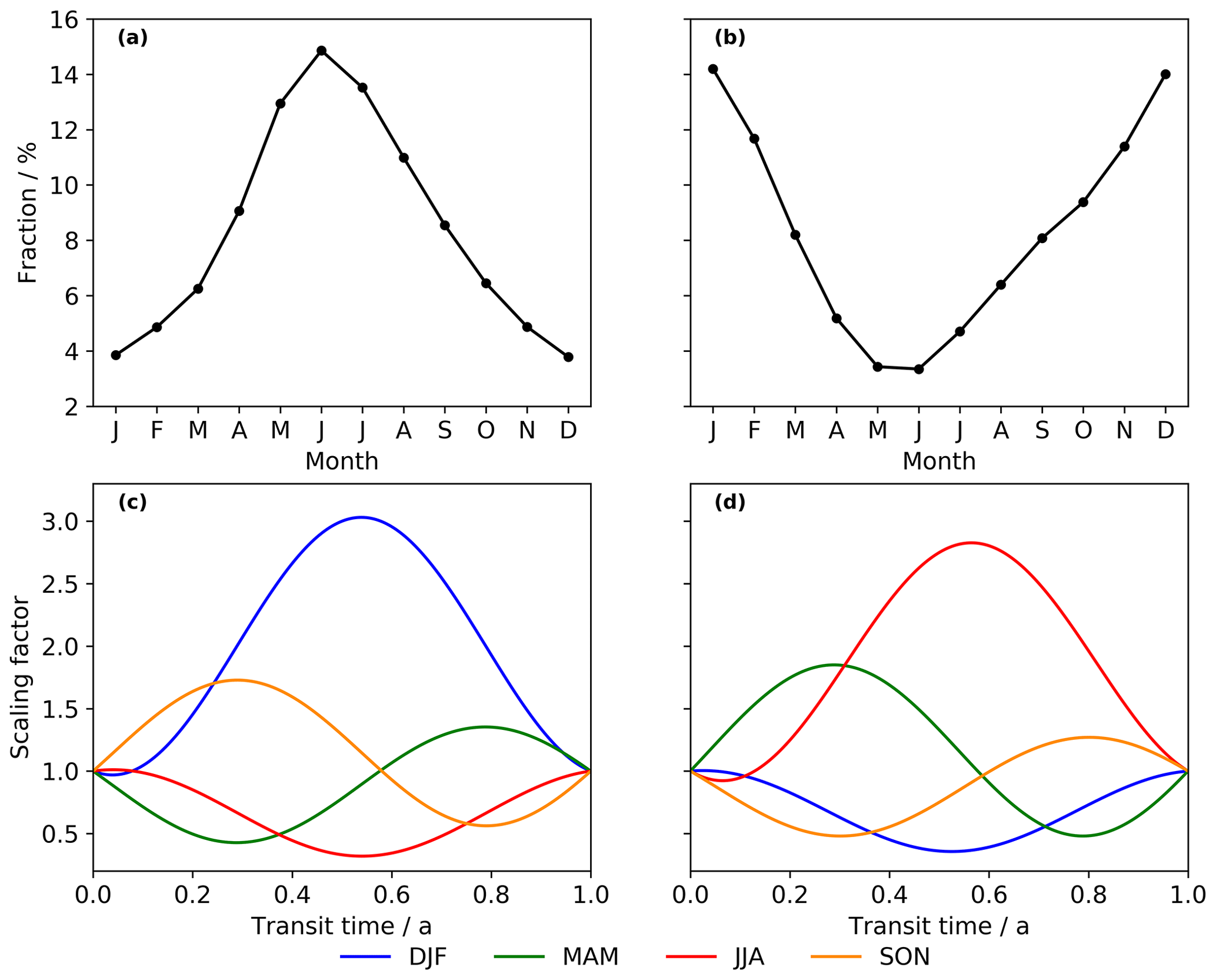
Figure 1The top row shows the fraction of air masses that enter the stratosphere in each month through the extratropical northern (30–90∘ N, panel a) and southern WMO tropopause (30–90∘ S, panel b) relative to all air masses entering through the defined regions within the CLaMS model simulation (see Sect. 3.1 for details). The fractions are calculated by bin-wise integration and summation of all global stratospheric GN (a) and GS (b). The bottom row depicts the approximated seasonal scaling factors for inverse age spectra referring to the northern (c) and southern (d) extratropical tropopause sections. Note that increasing transit time is equivalent to going backward in real time. Month-based abbreviations are used so that identical seasons have inverted colors in both hemispheres. See Sect. 2.2.2 for details on the derivation of the scaling factors. The fractions are normalized to equal 100 % when cumulated in each hemisphere.
The scaling factors are approximated from integrated CLaMS age spectra, which aggravates a comparison of higher-order peaks between the CLaMS reference and inverted age spectra as these modes are expected to appear at matching transit times. However, all global CLaMS age spectra are integrated and cumulated so that the resulting seasonality of the fractions is an average measure, and no information about the exact shape is transferred from CLaMS to the inverse method. All inverse age spectra in one specific season are moreover scaled with the same factor globally, which implies that the intrinsic amplitude of the monomodal inverse spectra must be well-retrieved as otherwise the scaling would nevertheless lead to deviating modes. Since the discovered seasonality in entrainment is also in good agreement with the upward ozone flux in the subtropical jet stream region (Yang et al., 2016) and with the seasonality derived from observations in the NH (Bönisch et al., 2009), the derived scaling factors are deemed a robust estimator for the presented extended inverse approach with the specified NH and SH tropopause sections.
2.2.3 Limitations
The extended inverse ansatz keeps the benefit of an inversion with a single parameter, but it also holds some disadvantages that require the use of output from atmospheric transport models. The goal of this study is to reduce the amount of necessary model output as much as possible for the inversion and evaluation of age spectra, but it must be stated clearly that it is not feasible to provide a method based solely on observations. While all can be well-retrieved and evaluated to investigate the BDC without explicit use of the origin fractions fi(x,t) from models, they must be known beforehand to calculate the composite age spectrum as a superposition of all . This piece of information must be provided by a model simulation. Also, the choice of a prescribed inverse Gaussian function might not be valid for any point in the stratosphere, particularly for cross-hemispheric PDFs (i.e., in the NH and vice versa). However, it is expected that the fractions of interhemispheric exchange are vanishingly low in the lowermost stratosphere, making those age spectra negligible. For the remaining distributions it is assumed that an inverse Gaussian shape provides a robust approximation of both tropical and extratropical age spectra with a low amount of necessary input data. This seems a valid approach as modeled tropical age spectra (Li et al., 2012; Ploeger and Birner, 2016) exhibit strong similarities with an inverse Gaussian function only with multiple modes. Still, the constrained shape might lead to inaccuracies to an unknown extent.
Above all, the performance of the inverse method depends crucially on the physically precise quantification of the chemical lifetime for each trace gas, since chemistry and transport show a strong interrelationship. Due to this close link, the lifetime is considered to be dependent on transit times along an average Lagrangian pathway through the stratosphere (Schoeberl et al., 2000). Although Hauck et al. (2019) demonstrate that due to the consideration of multiple trace gases in the optimization process a pseudo-random error of up to ±20 % in the chemical lifetime can be compensated for, the correct determination of the local lifetimes along transit time remains a considerable problem. A probable strategy could be an advancement of the ansatz by Holzer and Waugh (2015) where not only observations of (very) short-lived substances but also a set of long-lived trace gases are involved in a Monte Carlo simulation to derive lifetimes and age spectra in a stepwise fashion. The chemical lifetimes are hereby set to constant values, which describe chemistry effectively (see Sect. 2.2.4). This approach has the advantage that it reduces the influence of model output but relies on the goodness of the observations, especially for long-lived trace gases.
2.2.4 Statistical inversion process
The study of Holzer and Waugh (2015) provides the basis to derive a representative chemical lifetime for each substance from observational data together with statistical techniques. For that purpose, Eq. (12) has to be slightly tweaked. All transit-time-dependent lifetimes are replaced by the concept of effective stratospheric lifetimes . Those quantify chemistry for any given age spectrum along all relevant transport pathways effectively by a single scalar. This leads to
where is again parameterized by Eq. (3). The effective lifetime for any trace gas can be retrieved numerically based on a prior estimate of the age spectrum . If this is derived, a slightly modified version of the K-inversion algorithm will use the prior age spectrum and optimize the effective lifetime for each substance separately using the same numerical methods as above. This is the τ-inversion. The physical difference between Eqs. (12) and (14) lies in the transit time dependence of the mixing ratio. Using effective lifetimes, this gradient is different from the one in the original formulation for a specified age spectrum. However, since the final mixing ratio is identical in both cases, that fact is negligible. In the original form, Holzer and Waugh (2015) apply global tropospheric lifetimes for long-lived substances to gain the prior estimate of the tropospheric age spectrum. In the stratosphere, however, most trace gases undergo considerable chemical loss processes that cannot be estimated well by global lifetimes, which make additional information necessary. Therefore, (very) long-lived trace gases are considered together with short-lived species to constrain the age spectrum. For this study, we select five short-lived brominated trace gases (CH2Br2, CHBr3, CHCl2Br, CHClBr2, and CH2ClBr), five long-lived substances (CF2Cl2 (CFC-12), CF2ClBr (halon 1211), CF3Br (halon 1301), CH3Br, and N2O), and the very long-lived trace gas SF6, which has been frequently used as a dynamical tracer in the past. All these species were measured during past airborne research campaigns so that a solid data basis can be established.
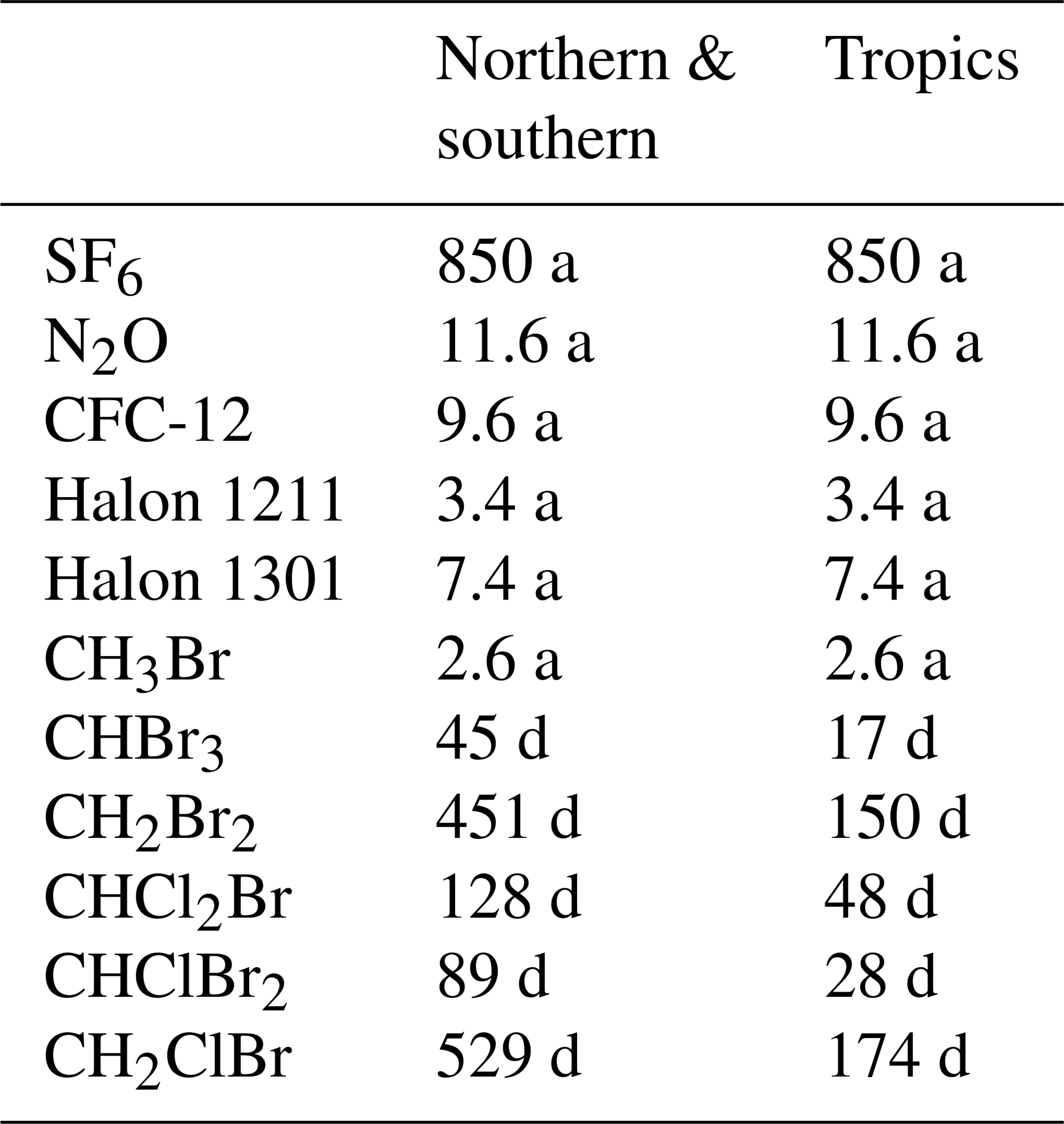
As stated above, the statistical inversion method requires a prior estimate of an age spectrum to infer the effective chemical lifetime. The outcome of the procedure hinges heavily on this first guess so that we introduce a Monte Carlo cross-validation (MCCV) for all tropopause sections to perturb the dependency and also consider a variety of uncertainties. As a first step, a subset of the trace gases is created, consisting of three selected species of the complete set. The subset is always composed of the dynamical tracer SF6, one of the five long-lived species, and one of the five short-lived species. The latter two are pseudo-randomly chosen. With this subset, the first guess of the age spectrum is constructed using the K-inversion on Eq. (14) together with an initial guess for the effective stratospheric lifetimes of the considered species. Other than in Holzer and Waugh (2015), a global lifetime is in general not suitable, as strong local stratospheric loss processes steer the effective lifetimes along all relevant transit times for both long- and short-lived trace gases. This implies that the effective lifetime of a species is generally smaller than its global lifetime. The exception is SF6, which has its main sink region in the mesosphere at large transit times. For the mainly short transport timescales in the lower stratosphere, the influence of the chemical loss is rather small, yet not negligible. The first-guess effective lifetime of SF6 is therefore set to be 850 years in accordance with Ray et al. (2017). In the case of the short-lived substances, mixing ratios are most probably steered by local chemical loss processes around the respective entry region. First-guess lifetimes for those species are taken as annual means from Tables 1–4 in Carpenter and Reimann (2014) for the NH and tropical tropopause sections. Long-lived trace gases show the most difficulties when assessing the first guess. On the one hand, global stratospheric lifetimes are likely an overestimation, as they are derived by dividing the global atmospheric burden by the global stratospheric loss rate. Local lifetimes, on the other hand, quantify the strength of localized stratospheric sink processes and thus do not consider that the desired lifetimes must express all relevant chemical depletion effectively for a given age spectrum. Additionally, these lifetimes are in many cases derived from model simulations. This study strives for a reduced model influence, so that the global stratospheric lifetimes from Table 5.6 in SPARC (2013) are turned into lifetimes that consider the stratospheric burden rather than the total atmospheric burden and treat them as first-order approximations of effective loss. The effective lifetime in our formulation is similar to a transit-time-integrated steady state but only considers trace gas burdens and sink processes above the tropopause. Since all mass above the tropopause consists of 10 % of the complete atmospheric mass (Volk et al., 1997), the stratospheric burden of a substance is assumed to contribute only 10 % to its global burden. Dividing burden by loss, this concept translates into lifetimes that are only 10 % of the global stratospheric lifetime. All implemented first-guess lifetimes are shown in Table 2.
Table 2Initial-guess effective lifetimes for all species in this study. The values are annual averages and taken from Ray et al. (2017), SPARC (2013) and Carpenter and Reimann (2014).
These values do not necessarily provide a valid representation so that systematic errors are included in the simulation. The errors were selected pseudo-randomly with uniform distribution for a random number of trace gases in the prior subset. They range from −50 % to +50 % for the first-guess lifetimes and from −σ to +σ for and χ(x,t). σ denotes the standard deviation of a mixing ratio (see Sect. 3.2 for details). After the prior age spectrum has been determined, it is used to perform the τ-inversion on Eq. (14) during which an effective lifetime is retrieved for every remaining substance that has not been in the prior subset. Again, pseudo-random errors between −σ and +σ for all and χ(x,t) are applied to this set. For solid Monte Carlo statistics, this procedure is repeated 2000 times to cover as many initial subsets as numerically feasible. There is no effective lifetime for SF6, since this tracer is present in every initial subset. That is done to make full use of SF6 as a reasonable frame for the age spectrum, which is then convoluted with further trace gas information to get an even more robust and unbiased prior. After completion of the Monte Carlo simulation, the median of the retrieved effective lifetimes is utilized in a final K-inversion for the full trace gas set to determine the desired age spectrum. SF6 is also not present in this final step to keep its direct influence restricted to the prior. In the rare case that no median effective lifetime can be derived for one of the remaining substances, the species will be omitted during the final K-inversion. To estimate the uncertainty range of the simulation, the lifetime of the 25th and 75th percentiles is taken to derive the upper and lower error margin of all age spectra and related moments.
Although that procedure is numerically expensive and requires multiple simulations for one set of mixing ratios at one location, the outcome of a reduced influence of model output seems promising. This comes at the cost of relatively large uncertainties for the retrieved effective lifetimes and age spectra, which hinge strongly on precise in situ measurements. With the considered errors in the Monte Carlo simulation, it is possible to receive an impression of the influence of these uncertainties on age spectra from observations.
3.1 CLaMS simulations
Two simulations with the Chemical Lagrangian Model of the Stratosphere (CLaMS) have been performed in a similar framework as the simulation of Ploeger and Birner (2016). CLaMS uses a Lagrangian perspective to model transport processes and chemistry for trace gases along calculated three-dimensional forward trajectories of single air parcels in combination with a parameterization scheme for small-scale mixing (McKenna, 2002a). That scheme leads to strong mixing in regions where deformations of the background flow are large (Konopka, 2004). CLaMS simulates transport in potential temperature space, where the vertical coordinate is designed as a hybrid between potential temperature in the stratosphere and upper troposphere and an orography-following pressure coordinate in the vicinity of the surface with smooth transition. The vertical speed along this coordinate is steered by the total diabatic heating rates from the reanalysis product that drives the simulation (Pommrich et al., 2014). In this study, CLaMS is driven by meteorological output of the ERA-Interim reanalysis (Dee et al., 2011). The final output of the Lagrangian model is gridded spatially with a resolution of 2∘ by 2∘ and 37 vertical potential temperature levels between 280 and 3000 K. Both simulations cover the period from January 1989 to December 2017 as a daily mean. Final model output is evaluated as zonal and seasonal means between December 1999 and November 2009 for the proof of concept.
This setup is suitable for the lower stratosphere, since fast transport processes across the tropopause are well-resolved. Age spectra in the model are derived from completely inert trace gases that are pulsed in certain intervals at the reference surface. Those pulse tracer series are then translated into proper spectra by the method of Ploeger and Birner (2016) for transient simulations. For convenience, these spectra are hereafter named pulse age spectra. In the first simulation (called TpSim), all tracers are initialized at the tropopause in the northern (90 to 30∘ N), tropical (30∘ N to 30∘ S), and southern (30 to 90∘ S) regions. Although a tropopause based on potential vorticity (PV) is a more suitable choice for dynamical studies, the simulations have been performed using the WMO definition of tropopause. For consistency between model and observations, tropopause hereafter always refers to the WMO definition. The tracer pulses are released as approximate Dirac delta distributions with a mixing ratio of 1 in their respective region and forced to zero when contacting the other two source sections. There are two separated sets of pulses for each source region to get a well-resolved age spectrum. They consist of 24 and 20 tracers, released monthly and semiannually, and cover a period of 2 and 10 years, respectively. If both sets are combined afterwards, the age spectrum will provide a fine monthly resolution up to 2 years and a coarser semiannual resolution for the remaining transit times up to 10 years. After every tracer has been pulsed once, they are reset and re-initialized.
The simulation also features three completely inert trace gases that are constantly released with a mixing ratio of 1 in the three source regions. These tracers provide the origin fractions for the reference surfaces without explicit integration of the age spectra. For the inverse method, 10 trace gases with spatially constant lifetimes ranging from 1 month to 109 months in steps of 12 months are included and released globally at the reference surface. The effective and transit-time-dependent lifetimes are identical for these radioactive tracers. The second simulation is a copy of TpSim, but with all substances being initialized at Earth's surface (called SurfSim) in the three specified regions. All age spectra from pulse tracers are extended to 50 years of transit time using the method described in Ploeger and Birner (2016).
3.2 Observational data
This study uses in situ measurement data obtained during two research campaigns of the High Altitude and Long Range Research Aircraft (HALO; http://www.halo.dlr.de, last access: 16 July 2020). The first campaign, PGS (Oelhaf et al., 2019), took place during December 2015 and March 2016, with the mission base in Kiruna, Sweden. PGS was a combination of the three missions POLSTRACC (Polar Stratosphere in a Changing Climate; https://www.halo.dlr.de/science/missions/polstracc/polstracc.html, last access: 16 July 2020), GW-LCYCLE (Gravity Wave Life Cycle), and SALSA (Seasonality of Air mass transport and origin in the Lowermost Stratosphere). PGS was split into two phases: the first from mid-December 2015 till late January 2016 and the second from late February 2016 till March 2016. The focus of PGS was strongly on the NH upper troposphere and lower stratosphere, as well as the exchange processes around the polar vortex and arctic latitudes. The second campaign, WISE (Wave-driven Isentropic Exchange; http://www.wise2017.de, last access: 16 July 2020), took place between September and October 2017, with the mission base in Shannon, Ireland. The focus of WISE was on isentropic exchange processes between the troposphere and stratosphere around the midlatitude tropopause. The flight tracks for both campaigns are shown in Keber et al. (2020). The campaign data are binned into grids of equivalent latitudes (Allen and Nakamura, 2003) and potential temperature differences to the WMO tropopause, with a bin size of K and treated as phase averages. Bins containing fewer than five data points are omitted. The standard deviation for all mixing ratios is derived during the binning procedure. All halogenated trace gases mentioned in Sect. 2.2.4 were measured by the Gas Chromatograph for Observational Studies using Tracers – Mass Spectrometer (GhOST-MS) operated aboard HALO. GhOST-MS is a dual-channel gas chromatograph coupled with an electron capture detector (ECD) in an isothermal channel and a quadrupole mass spectrometer (MS) in a temperature programmed channel. The setup and relevant precision values are given in Keber et al. (2020). All GhOST-MS data in this study are reported on SIO-05 scales. N2O was measured during PGS by the TRIHOP instrument (Schiller et al., 2008), an infrared absorption laser spectrometer with three quantum cascade lasers. The setup for PGS and respective precision values are described in Krause et al. (2018). During WISE, N2O was measured with the UMAQS instrument (Müller et al., 2015), also an infrared quantum cascade laser spectrometer. The setup for WISE and relevant precisions are given in Kunkel et al. (2019). These N2O data are reported on the WMO 2006a scale.
An important parameter for the inversion is the entry mixing ratio time series at the specified tropopause sections. We only derive entry mixing ratios for the NH and tropical tropopause, as we show in Sect. 4.1 that the influence of cross-hemispheric transport is negligible. The time series should cover the period from 1960 until November 2017 to retrieve a mathematically precise age spectrum with a range of 50 years of transit time. Unfortunately, there are no consistent measurements available covering the complete period at the surface let alone at the tropopause. That is problematic for the long-lived trace gases in this study (SF6, N2O, CFC-12, halon 1211, halon 1301, and CH3Br), since a strong long-term trend is detected at the surface. To construct a time series for these species, data from the Atmospheric Lifetime Experiment (ALE), the Global Atmospheric Gases Experiment (GAGE), and the Advanced Global Atmospheric Gases Experiment (AGAGE) (Prinn et al., 2018, 2019a) are taken and extended backwards until 1960 with global data from the Representative Concentration Pathways (Meinshausen et al., 2011a) for the two stations Ragged Point in Barbados (RPB – 13∘ N, 59∘ W) and Cape Matatula in American Samoa (SMO – 14∘ S, 171∘ W). The RCP data are aligned for any substance to suit the general behavior of the corresponding full ALE/GAGE/AGAGE data set but only considered where no measurements are available. All relevant data are reported on SIO-05 scales, except N2O, which is reported on both SIO-98 (ALE/GAGE) and SIO-16 (AGAGE). Despite the different scale names, N2O data on SIO-98 and SIO-16 scales are comparable. Both scales are considered to be comparable to WMO 2006A for the purpose of this study (World Meteorological Organization, 2018). Minor temporal gaps are interpolated. It is assumed that the long-lived gases are well-mixed, so that the average of RPB and SMO represents a tropical mixing ratio. As the global tropospheric lifetimes of these trace gases are sufficiently large, except for CH3Br (1.6 years according to Table 5.6 in SPARC, 2013), the extended ALE/GAGE/AGAGE data are lagged to the tropical tropopause by 2 months ±0.5 months. The validity of that approach is shown in Andrews et al. (1999) with CO2 data. In the case of CH3Br, some chemical loss processes might already occur while propagating towards the tropopause, but since the time lag is still much smaller than the global tropospheric lifetime, the lagged mixing ratio is assumed to be representative.
For the NH tropopause section, the net flux across the section is downward (Olsen et al., 2004), so that tropospheric air mixes with descending stratospheric air, characterized by lower mixing ratios due to the chemical loss regions in the stratosphere. At the extratropical tropopause the mixing ratio should thus be lower than in the tropics. Additionally, the trace gas burden at the extratropical tropopause consists of a mixture of air from the tropics and extratropics, aggravating a straightforward lag approach. The tropical origin fraction from the CLaMS simulation SurfSim provides a suitable tool to characterize the most important surface source section. The annual mean origin fraction indicates that at the NH tropopause section, approximately 88±4 % of all air masses originate from the surface in the tropics, with a corresponding mean AoA of 1 year ± 0.25 years. All tropical ALE/GAGE/AGAGE data are lagged by this value to retrieve the mixing ratio time series at the NH extratropical tropopause. Since the main sink of CH3Br in the troposphere is the temperature-dependent reaction with the hydroxyl radical, chemical loss processes in the cold middle and upper troposphere are again treated as first-order negligible compared to the transport timescale. The standard deviation for these time series is derived from the respective measurement error and the deviation that emerges when the uncertainty of the lag time is implemented, especially relevant for RCP data as these do not provide a measurement error. The short-lived species (CH2Br2, CHBr3, CHCl2Br, CHClBr2, and CH2ClBr) show weak long-term trends at the tropopause. For the tropics, the mixing ratios of the upper TTL in Tables 1–4 of Engel and Rigby (2019) are considered to be the annual mean entry mixing ratio, as the potential temperature range matches the WMO tropopause of ERA-Interim in the specified tropical region. The mixing ratios at the NH tropopause section are taken directly from the PGS and WISE data, which are averaged between 30 and 90∘ N of equivalent latitude and between the tropopause and 30 K above, as this is specified as a region of strong tropospheric influence (Hoor et al., 2004). The large interval of 30 K has been introduced to incorporate the strong seasonal variability of the WMO tropopause in the NH throughout the year into the mixing ratios and to regard general discrepancies between the dynamical (PV-based) and WMO tropopause. To be consistent, the first 30 K above the tropopause is then omitted in the inversion procedure. The uncertainty values for all short-lived substances at the NH tropopause section are derived as the standard deviation from the average. In the tropics, the standard deviation given by Engel and Rigby (2019) is applied.
4.1 Origin fractions for different entry regions
Origin fractions are a valuable tool to quantify the importance of air entrainment through each specified tropopause section and cross-hemispheric transport for air mass composition in the stratosphere. Figure 2 shows global cross sections of all annually and seasonally averaged origin fractions from TpSim as a function of potential temperature and latitude. The model setup is consistent overall, as the fractions at each location sum up to circa 100 % in the stratosphere. On annual average, the general distribution of the origin fractions resembles the pattern of the BDC quite well with strong upwelling in the tropics and a downward motion at NH and SH extratropical latitudes. The sharp borders of all fractions at the tropopause around 30∘ N and S are caused by the definition of the source regions in the model. It is apparent that the tropical tropopause constitutes the predominant source region for the complete stratosphere above 450 K, with the tropical origin fraction (panel “Annual” in middle row) reaching more than 70 %. Below 450 K, the NH (panel “Annual” in top row) and SH (panel “Annual” in bottom row) tropopause sections gain significant influence in the extratropics, manifesting in a rise of the respective origin fractions when approaching the tropopause. Cross-hemispheric transport is negligible, since the northern fraction in the SH and the southern fraction in the NH are vanishingly low and only reach values up to 10 %. Therefore, the corresponding cross-hemispheric age spectra can be omitted as they contribute only marginally to the composite spectrum. Both the NH and SH origin fractions show a sharp latitudinal gradient directly at the Equator accompanied by a strong increase in the tropical fraction, visible as a beam of deep red shading around the Equator throughout the stratosphere. This might be an effect of the subtropical transport barriers that enclose the tropics, separate them from the extratropics, and inhibit exchange processes (Neu and Plumb, 1999).
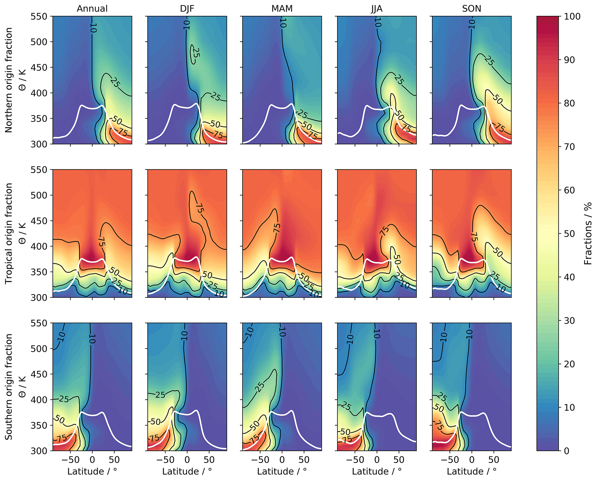
Figure 2CLaMS origin fractions from TpSim as annual (left column) and seasonal (remaining four columns) mean global cross sections from the northern hemispheric (top row), the tropical (middle row), and the southern hemispheric (bottom row) tropopause source region (for definition see text). The solid white line indicates the WMO tropopause from ERA-Interim output. Negative latitudes always denote the Southern Hemisphere.
All origin fractions undergo a pronounced seasonality (panels DJF to SON in all rows). For the NH fraction (top row), the maximum above the tropopause is visible in SON reaching up to almost 500 K in the tropics with extensive values between 50 % and 75 % in the lower stratosphere up to circa 380 K, while the minimum is found with a 6-month offset in MAM. JJA and DJF show a transition state between the maximum and minimum, which follows the seasonality of the mass fluxes in Sect. 2.2.2. As it takes some time for the air to propagate from the NH tropopause section upward into the stratosphere, the maximum NH origin fraction, i.e., a flushing of the NH with fresh tropospheric air, is modeled with some delay in SON. The same principle applies to the minimum of the NH fraction. Since the maximum downward forcing through the 380 K level is simulated in late January, the NH origin fraction attains its minimum in MAM. The isolated area of enhanced NH fraction at circa 380 K and 30∘ N in JJA could be related to the Asian summer monsoon, which is known to transport fresh air into the NH (sub)tropical stratosphere (Vogel et al., 2019) and matches well with the findings of Yang et al. (2016). For the SH origin fraction (bottom row), the correlation with the mass flux is not as clear as in the north. Intuitively, maxima and minima should be shifted by 6 months, with maximum SH fraction in MAM and minimum in SON. While the fraction in MAM appears strongest between 30 and ca. 55∘ S in the lower stratosphere with a pronounced vertical structure and values of 40 % to 75 %, a large area of strongly enhanced SH fraction (up to 75 %) is visible in SON at high latitudes. This is most likely linked to the initialization of the tracers at the WMO tropopause, which is found at high altitudes due to the very low temperatures inside the SH polar vortex. Apart from that, seasonal fluctuations seem weaker in general for the SH fraction. The tropical origin fraction in the lower stratosphere shows the weakest seasonality and spreads deep into the extratropics with values around 70 % to 80 % during minimal phases of the NH and SH fraction (especially MAM and JJA in the north and JJA and SON in the south, which is in accordance with the results of Hegglin and Shepherd, 2007). The maximum of the tropical fraction follows the tropical upward mass flux (Rosenlof, 1995) and shifts from the southern edge of the tropics in JJA to the northern edge in DJF, with the latter showing a slightly broader structure. The presented origin fractions reveal that the assumption of single entry through the TTL appears robust in the tropics and above 450 K globally. Age spectra, however, will lack important features of stratospheric transport in the extratropical lower stratosphere if only the tropical section is considered. To retrieve a precise composite age spectrum in both the model and inverse method, the tropical and the respective extratropical spectrum, north or south, must be determined and superimposed. Since the influence of cross-hemispheric transport is vanishingly low, the related cross-hemispheric age spectra are now omitted to simplify the setup.
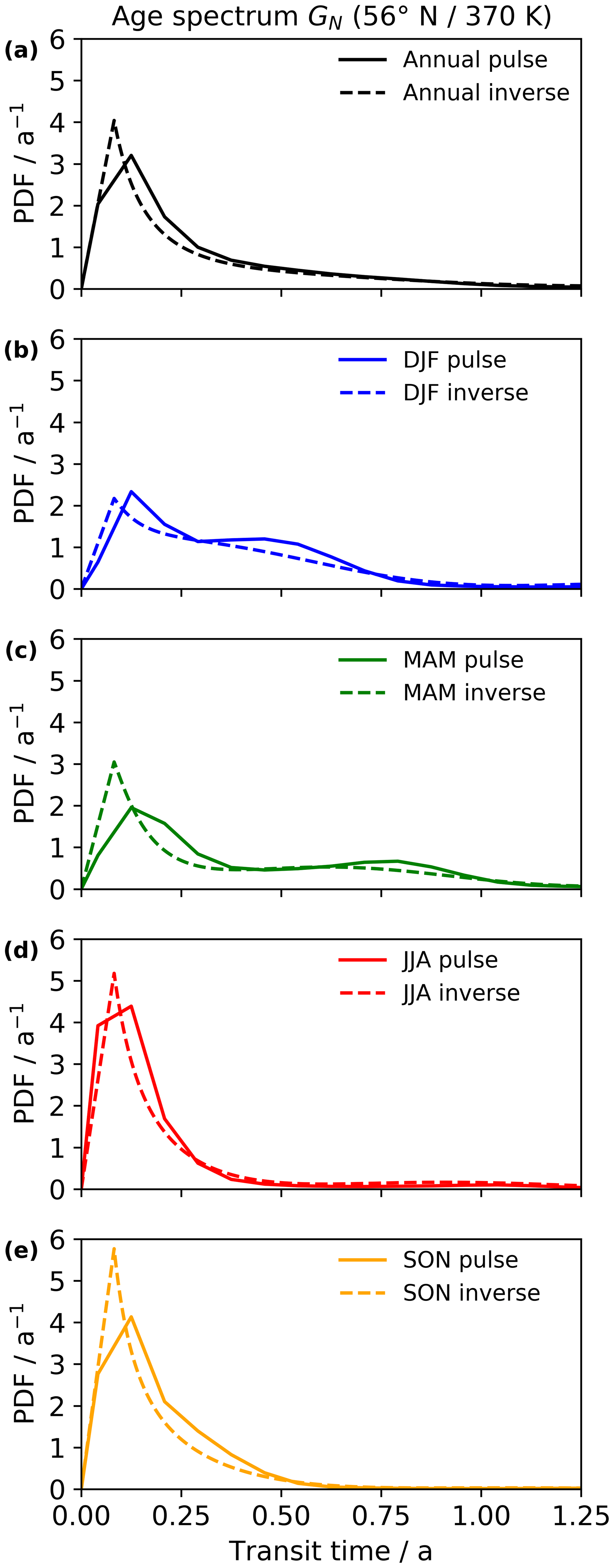
Figure 3Normalized age spectra with reference at the northern hemispheric tropopause region GN at 56∘ N and 370 K as annual (a) and seasonal (b–e) means. The solid line denotes age spectra from CLaMS pulse tracers, and the dashed line denotes inverse method age spectra.
4.2 Proof of concept
4.2.1 Age-of-air spectra
Hauck et al. (2019) provide an extensive proof of the inverse concept for the age of air for the tropical tropopause entry, so this study focuses on the NH and SH spectra in the midlatitudes of the respective hemisphere close to the local tropopause. All presented age spectra are normalized to avoid dependency on the CLaMS origin fractions. Figure 3 shows the normalized pulse (solid lines; see Sect. 3.1 for details) and inverse age spectra from the radioactive tracers (dashed lines; see Sect. 2.2.1 and 2.2.2 for details) with reference at the NH tropopause at 56∘ N and 370 K as annual (black) and seasonal (colored) means. To ease comparison, transit times below 1 month are excluded from all inverse spectra, as this is the minimum resolution the pulse tracer experiment provides. The annual mean inverse spectrum (panel a) matches well with the pulse spectrum and exhibits a very similar shape with one pronounced peak at similar transit times and no further modes. This indicates that the seasonal scaling works properly as it cancels out on annual average. The amplitude of the inverse spectrum is slightly larger than the pulse spectrum, although it appears as if the mode of the pulse spectrum is clipped off by the 1-month resolution, leading to a slightly right-tilted peak. A more frequent pulsing of the tracers could improve the alignment of the inverse method and pulse spectra. For the seasonal spectra (panels b to e), the performance of the inverse method and its coupled seasonal scaling factor seems robust. Although the scaling factor is derived from the seasonal cycle in CLaMS and thus is expected to produce matching modes, the amplitude of the monomodal inverse spectra must be well-retrieved as otherwise the scaling would lead to deviating peaks and troughs. The amplitude of the first mode is well-reproduced in DJF and JJA, while MAM and SON are overestimated by approximately 50 %. Just as for the annual mean, the pulse spectra primary peak in MAM, JJA, and SON and in DJF appear to be slightly cutoff by the resolution of the tracer pulsing with a similarly right-tilted shape. Even though the shown NH seasonal inverse spectra are independent of the respective CLaMS origin fraction, they correctly reproduce a maximum of air entrainment in the JJA and SON spectra with almost twice as large maxima (5.18 and 5.77 a−1) as in DJF and MAM (2.17 and 3.05 a−1). This follows the maximum of the NH origin fraction in Fig. 2 (SON) very well and implies that the inverse spectra correctly reproduce the seasonality in cross-tropopause transport in the NH without explicit consideration of the fraction.
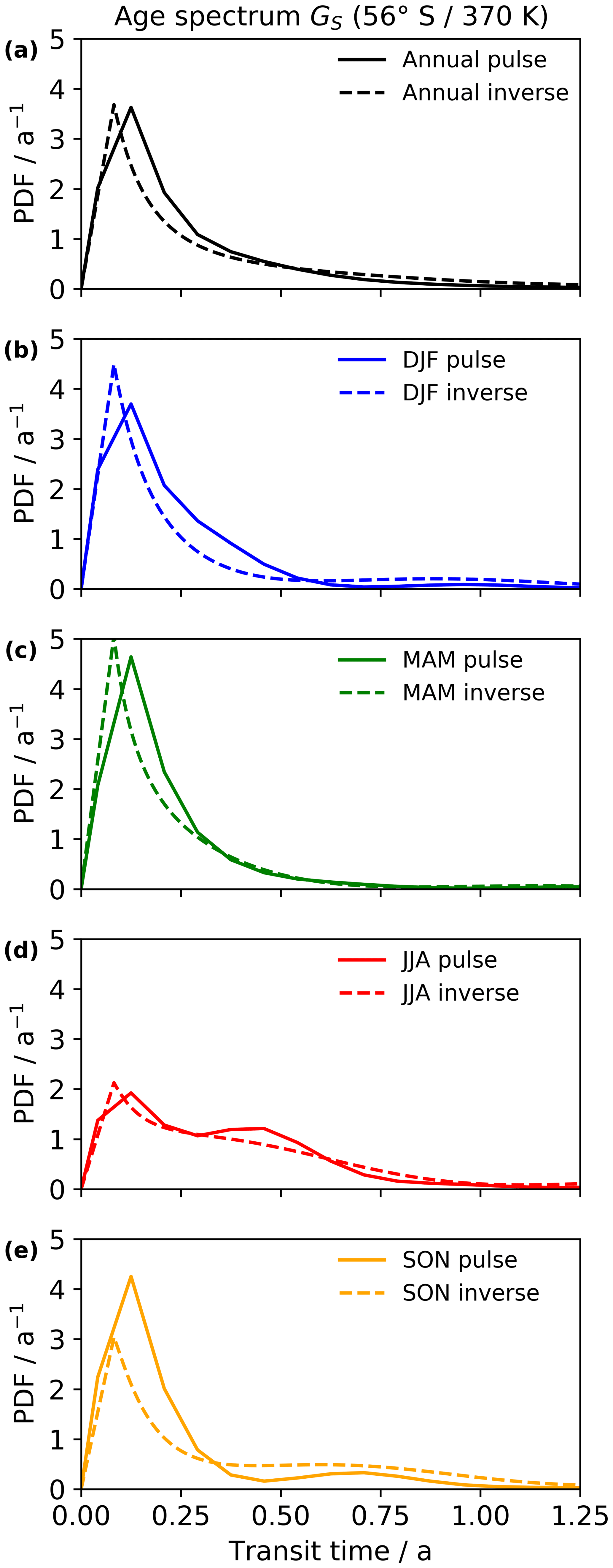
Figure 4Normalized age spectra with reference at the southern hemispheric tropopause region GS at 56∘ S and 370 K as annual (a) and seasonal (b–e) means. The solid line denotes age spectra from CLaMS pulse tracers, and the dashed line denotes inverse method age spectra.
Figure 4 correspondingly displays the normalized CLaMS pulse (solid lines) and inverse (dashed lines) age spectra at 56∘ S and 370 K as annual (black) and seasonal (colored) averages with origin at the SH tropopause. The performance of the annual mean inverse spectrum (panel a) is similar to that of the NH spectrum with slightly better agreement of the main mode amplitude. The timing of the main peak coincides again with the pulse spectra. No further modes are visible in annual mean pulse and inverse spectra, indicating that the SH scaling factor seems to also work as intended on an annual scale. The right-tilted shape of the pulse spectrum peak indicates that some features of transport are clipped off in the spectra due to its transit time resolution. On the seasonal scale (panels b to e), the inverse method reproduces the general shape of the pulse spectra a bit better than in the NH, with well-matching primary modes. Only in SON is the pulse spectra amplitude underestimated by circa 25 %. This might be related to the WMO tropopause in this region. Consistently, all seasonal pulse spectra suffer from the same cutoff effect at small transit times as the NH spectra. Higher-order maxima and minima of the inverse spectra are in good agreement with the pulse spectra, which is expected as for the NH spectra above. During SH winter (JJA), a similar underestimation of the amplitude is visible as in NH winter (DJF) of Fig. 3. This might be related to the assumed inverse Gaussian shape. In terms of transport seasonality, the inverse age spectra follow the SH origin fraction again quite well without considering them explicitly. The maximum of transport is visible in the DJF and MAM spectra with amplitudes of 4.49 and 5.07 a−1, while JJA and SON constitute phases of weaker transport (2.13 and 3.04 a−1). Compared to the NH, the seasonality is in general not as strong and pronounced, similar to the seasonality of the SH fraction (Fig. 2).
Despite its restriction to an intrinsically inverse Gaussian shape, the extended inverse method with the newly introduced extratropical scaling factors appears to retrieve precise age spectra in the NH and SH midlatitude lower stratosphere if chemical lifetime and mixing ratios are well-constrained. All derived inverse age spectra then capture important features of transport from the CLaMS model on a seasonal scale without direct influence of the modeled origin fractions.
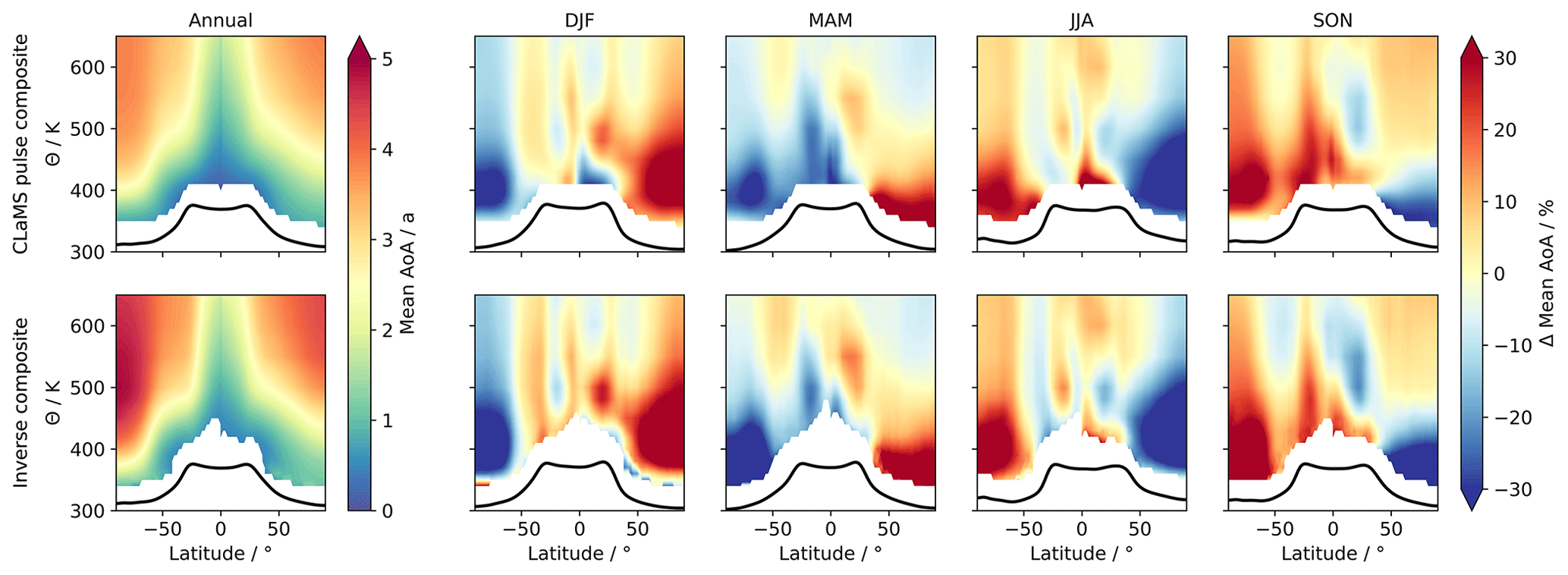
Figure 5Global cross sections of mean age of air derived from the CLaMS pulse composite age spectra (top row) and from the inverse composite spectra (bottom row). The first column shows absolute values as the annual mean, and the right four columns show seasonal percentage differences relative to the annual mean. In all panels, the black line indicates the tropopause. The composite age spectra are calculated for this specific comparison using only annual mean origin fractions of the CLaMS model to focus explicitly on seasonality in mean AoA. Note that in the bottom row the larger areas of undefined values at the tropical tropopause are caused by the inversion algorithm not finding a valid solution for the transport parameter in that region. The first 30 K above the tropopause is omitted in all panels.
4.2.2 Mean age of air
For a full global-scale assessment, Fig. 5 shows cross sections of mean age of air derived from the composite pulse (top row) and composite inverse age spectra (bottom row). The first column (annual) shows annual mean absolute values, while the remaining four columns (DJF to SON) depict seasonal percentage differences relative to the respective annual average. Although a tropopause-relative coordinate system is generally preferable for an analysis of mean AoA close to the tropopause to incorporate the variable tropopause height throughout the year, absolute coordinates are chosen for this comparison to ease comparability with Fig. 8 in Hauck et al. (2019). Changes in tropopause height should affect the data in both rows of the figure similarly so that a comparison between CLaMS pulse and inverse mean AoA is not inhibited. A seasonal analysis of the composite spectrum is advantageous to assess the behavior of all three different age spectra – northern, tropical, and southern – simultaneously, but weighted by their geographical importance. Since all origin fractions undergo a distinct seasonality, which is not necessarily identical with the seasonality of the age spectra, the composite spectrum of CLaMS pulse spectra and the inverse method is calculated for this specific comparison only with annual mean origin fractions in Eq. (8) (inserted into Eq. 6). This ensures that the presented seasonal differences are only steered by the inverted age spectra and preserves the weighting of the individual age spectra at the same time. On annual average, good agreement between inverse and pulse mean AoA is detected, where both show very similar spatial structures. The inverse method correctly reproduces the low mean AoA values of the pulse mean AoA in the tropics and the positive gradient towards the poles. Even the area of enhanced mean AoA at high SH latitudes between 400 and 500 K is emulated, although it extends down below 380 K. The inverse mean AoA is generally biased and exhibits larger mean AoA than the pulse spectra. This fact is in accordance with the results of Hauck et al. (2019), who also found an overestimation of mean AoA by the inverse method and link it to the prescribed inverse Gaussian shape of the age spectra. To quantify comparably in this study, the globally averaged bias both above and below a threshold of 1.5 years of mean AoA is retrieved (see Hauck et al., 2019, for details on the threshold). We find that the deviation decreases from +44.3 % below the threshold in Hauck et al. (2019) to only +13.8 % in this study. Above, the bias remains almost steady at +12.4 % compared to +13.3 % before. This improvement demonstrates the benefit of the extended approach, although some improvement might also be attributed to the finer pulse resolution, especially around the tropopause.
Seasonal differences give a similar impression with spatial patterns of inverse mean AoA that match those of the pulse mean AoA in the stratosphere qualitatively well. Only the amplitude of the differences appears enhanced for the inverse method, e.g., the darker shading of red at 50∘ S and 600 K in SON, but coincides with the detected bias on the annual scale. In the lower stratosphere, all positive and negative fluctuations are correctly retrieved by the inverse method. That is an improvement over Hauck et al. (2019), as they found inverted seasonal structures, i.e., positive seasonal differences in the pulse and negative differences in the inverse mean AoA, in the NH lower stratosphere during MAM and SON. Only in DJF directly above the tropopause in the NH midlatitudes and at the south pole does the sign appear different. That might be an artifact of the close proximity to the tropopause where an inverse Gaussian shape might not resemble the pulse spectrum correctly. Both pulse and inverse mean AoA exhibit a flushing of the subtropical and extratropical lower stratosphere with fresh tropospheric air during summer and fall of the respective hemisphere. That coincides well with the season of maximum amplitude of the NH and SH age spectra in Figs. 3 and 4 and shows their importance for a seasonally precise description of transport in the lower extratropical stratosphere. In the tropics, the maximum of tropospheric air is visible in MAM, but some strong entrainment is already visible around 30∘ N in DJF and around 30∘ S in JJA. This follows the seasonality of the tropical origin fraction in the tropics shown in Fig. 2 without explicit inclusion of the seasonal factors in the composite age spectrum.
The results of the idealized proof of concept demonstrate the significantly improved performance of the extended inverse ansatz for age spectra in the lower extratropical stratosphere, which has previously been identified as a critical region for the tropical age spectra by Hauck et al. (2019). The inverse method retrieves the NH and SH age spectra correctly and the newly inferred seasonal cycles impose modes at transit times that correspond to the CLaMS pulse age spectra very well both locally in the NH and SH midlatitudes and on the global scale as a composite with the tropical spectra. In its extended state, the inverse method can probably provide insight into transport mechanisms involving the tropical and extratropical tropopause. However, since this section provided only a highly idealized test scenario, the performance of the method and the statistical retrieval procedure for chemical lifetimes is assessed under more realistic conditions in the next sections.
4.3 Observational data
4.3.1 Mean age of air
The focus of the following sections is on the application of the inverse method to in situ measurements of 11 chemically active trace gases (SF6, N2O, CFC-12, halon 1211, halon 1301, CH3Br, CH2Br2, CHBr3, CHCl2Br, CHClBr2, and CH2ClBr) taken during the two aircraft campaigns PGS (phase 1 in winter 2015/2016, phase 2 in early spring 2016) and WISE (fall 2017). Results are evaluated under consideration of findings in previous studies. Note that the following sections use solely equivalent latitude as horizontal and potential temperature difference to the local tropopause as the vertical coordinate. All presented age spectra are independent of any modeled origin fractions. Figure 6 depicts cross sections of mean AoA from the normalized inverse age spectra referring to the NH entry (top row) and tropical tropopause entry (middle row) during PGS phase 1 (first column), PGS phase 2 (second column), and WISE (third column). The absolute difference between NH and tropical mean AoA is shown in the bottom row of the figure. The spatial distribution and quantitative range of inverse mean AoA in both rows appear meaningful and coherent in general, showing smaller values towards the tropics and an increase with latitude and altitude. For PGS phase 1 and PGS phase 2, the spatial distribution seems consistent with the data in Fig. 3 of Krause et al. (2018), although their observational-based mean AoA values refer to Earth's surface in the tropics and therefore regard transport across both tropical and NH tropopause regions. The quantitative range of mean AoA in Krause et al. (2018) should be larger than in this study, as tropospheric transport up to the tropopause sections is included in their mean AoA.
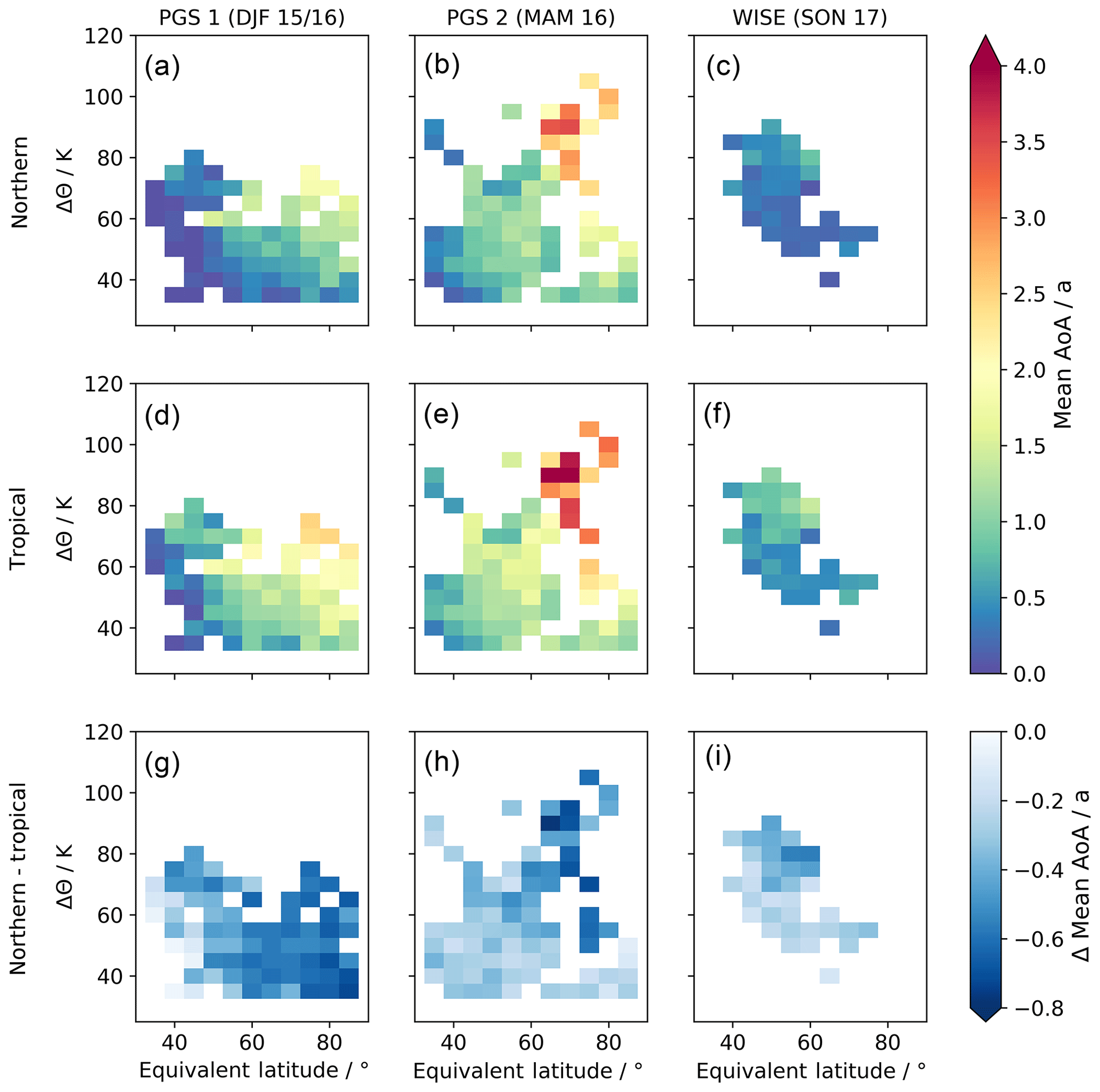
Figure 6Cross sections of binned mean age of air calculated using the age spectra retrieved with the inverse method in the Monte Carlo simulation (see Sect. 2.2.4). The top row shows mean AoA referring to the northern hemispheric tropopause section, while mean AoA in the middle row refers to the tropical tropopause section. The left column displays data of PGS phase 1, middle column data of PGS phase 2, and right column data of WISE. The bottom row gives the absolute differences between the data in the top and middle rows. The potential temperature difference to the local tropopause ΔΘ is used as the vertical coordinate and equivalent latitude as the horizontal coordinate.
Mean AoA referring to the NH tropopause (top row) is found to show the largest values of all data during PGS phase 2 with scattered bins of mean AoA older than 3 years around 90 K and 75∘ N. While both PGS phase 1 and PGS phase 2 cover a wide latitudinal range from 35 up to 85∘ N, WISE is strongly confined and centered around 50∘ N with vertical extent similar to PGS 1. For WISE, mean AoA is slightly smaller than during PGS in the same spatial region. Minimum inverse mean AoA values of all three campaigns are retrieved for PGS phase 1 between 40 and 45∘ N below 50 K and even below 40 K at circa 70∘ N with bins of less than 0.1 years. This implies a strong entrainment of fresh tropospheric air into the lowermost stratosphere across the NH tropopause during summer and fall. On the one hand, this manifests in already diminished mean AoA during WISE, i.e., early fall 2017, and, on the other hand, in minimum mean AoA values for PGS phase 1, i.e., winter 2015/2016, where air that entered prior to the campaign already had some time to propagate upward from the tropopause. That seasonality in local entrainment across the tropopause is consistent with the results of the SPURT aircraft campaign in Fig. 6 of Bönisch et al. (2009), showing a maximum of air with tropospheric origin in the lowermost stratosphere in October (> 80 %) and a minimum in April (< 20 %) due to strong local quasi-isentropic mixing processes across the subtropical jet stream in summer and fall.
Mean AoA referring to the NH tropopause is generally smaller than the tropical counterpart, with an average difference ranging from −0.3 years for WISE to −0.36 years for PGS phase 2 and −0.46 years for phase 1. The difference is smaller at lower latitudes and increases with latitude and distance from the tropopause (see bottom row). Maximum mean AoA of tropical origin (middle row) is retrieved for PGS phase 2 with values of more than 4 years but with a larger vertical extent down to 55 K at 75∘ N. Similar to above, minimum mean AoA in the midlatitudes between 50 and 70∘ N is found during WISE, but only slightly smaller than during PGS. The absolute minimum of mean AoA during all campaigns is retrieved again in PGS 1 (∼0.1 years at 40∘ N and 50 K), although the spatial distribution of the minimum is much more confined to low latitudes than for mean AoA with the NH tropopause as reference. The generally lower mean AoA values derived during WISE with origin at the tropical tropopause are expected, as NH winter is characterized as the season where the tropical upward mass flux attains its maximum (Rosenlof, 1995). Therefore, entry of fresh tropospheric air through the tropical tropopause peaks during NH winter and manifests in lower mean AoA with some delay during JJA and SON in the NH extratropical lowermost stratosphere.
Although these findings coincide robustly with results of previous studies, the strong similarity between the spatial distribution of mean AoA with NH and tropical tropopause as reference is quite nonintuitive. Since transport processes to a specified location starting at the NH extratropical tropopause should be different from those beginning at the tropical tropopause, one could expect that mean AoA fields are more individually shaped. To check that this is not caused by the inversion concept in general, the raw model output of CLaMS TpSim (see Sect. 3.1) has been interpolated onto the HALO flight tracks for PGS and WISE. CLaMS pulse mean AoA fields are shown together with the corresponding inverse mean AoA in Figs. S1 and S2 in the Supplement to this study. Results reveal that CLaMS models a similarity between mean AoA with origin at the NH and tropical tropopause analogous to the inverse method based on observational data.
4.3.2 Campaign-averaged age-of-air spectra and mean age of air
Figure 7 presents the campaign-averaged age spectra derived by the inverse method with reference at the NH tropopause (panel a) and tropical tropopause (panel b) for PGS phase 1 (DJF, blue), PGS phase 2 (MAM, green), and WISE (SON, orange). To ensure comparability, the campaign average is constructed by selecting only bins that are present in both PGS phases and WISE. Shaded areas denote the derived uncertainty range from the Monte Carlo simulation (see Sect. 2.2.4 for details). For the inverse spectra with reference at the NH tropopause, the maximum amplitude is detected during WISE (8.81 a−1), followed by PGS phase 1 (4.65 a−1) and PGS phase 2 (1.09 a−1). The transit times at the spectra maxima (i.e, modal age) come out equally for WISE and PGS phase 1, both around 0.5 months. This implies that a flushing event with extratropical tropospheric air due to mixing across the NH tropopause section is retrieved for early fall 2017 prior to WISE and early winter 2015/2016 prior to PGS phase 1. That is corroborated by the inverse spectrum for PGS phase 2, which displays its first mode at a modal age of circa 2 months, equivalent to midwinter 2015/2016. While the age spectrum for WISE rapidly decreases after its primary mode and reaches its first minimum at circa 0.8 years of transit time, the inverse age spectra during PGS phases 1 and 2 exhibit a saddle point up to transit times of 0.5 and 0.75 years, respectively. However, those secondary peaks are parametrized by the seasonal scaling factor and can therefore not be considered as a real signal of transport. Mean AoA values for the spectra in panel (a) of Fig. 7 are shown in panel (a) of Fig. 8 and quantitatively emphasize the seasonality in transport visible on a larger scale in Fig. 6. For WISE, mean AoA is retrieved to be considerably lower (0.25 years) than for PGS phase 1 (0.7 years) and phase 2 (1.10 years), which is in accordance with the seasonality found by Bönisch et al. (2009) for the SPURT campaign.
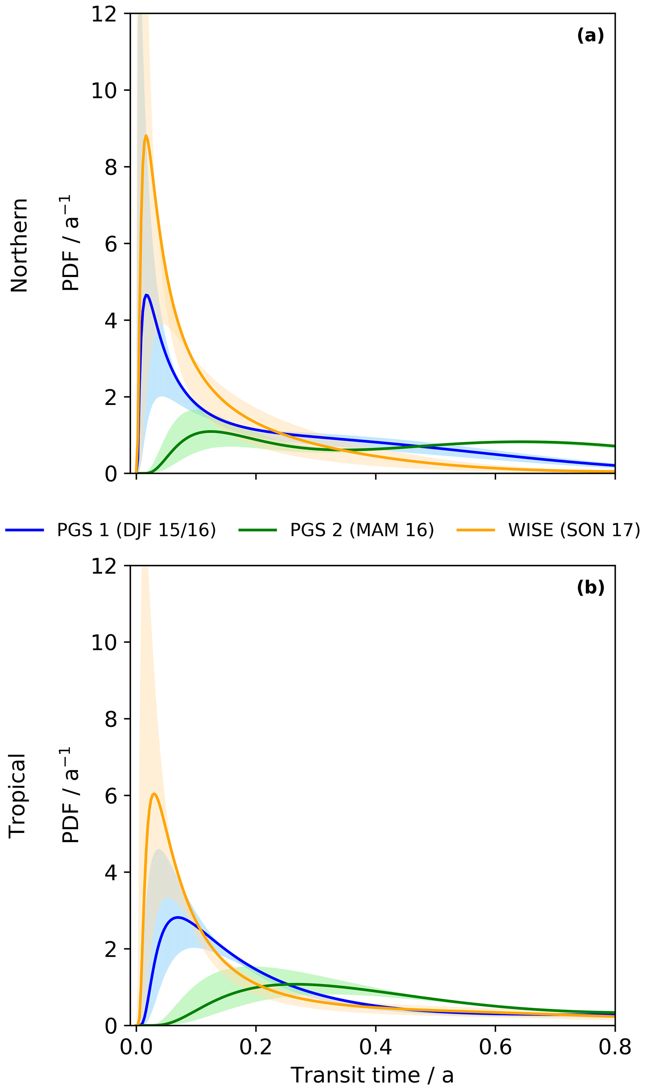
Figure 7Campaign-averaged age spectra for PGS phase 1 (blue), PGS phase 2 (green), and WISE (orange). Panel (a) shows normalized inverse age spectra GN referring to the northern hemispheric tropopause section, while (b) shows normalized inverse age spectra GT referring to the tropical tropopause section. Colored shadings give the uncertainty range of the spectra derived from the Monte Carlo simulation (see Sect. 2.2.4 for details).
All primary modes of the age spectra with origin at the tropical tropopause show smaller amplitudes and generally broader peaks compared to the northern counterparts but with an identical order of the campaigns. The maximum is found for WISE (6.04 a−1), followed by PGS phase 1 (2.81 a−1) and PGS phase 2 (1.07 a−1). Modal ages are similar for WISE and PGS phase 1, both with circa 1 month. For PGS phase 2 an increase is visible, reaching a modal age of 3 months. These age spectra imply that entry of fresh tropospheric air through the tropical tropopause has peaked in early fall 2017 and also early winter 2015/2016 but is less strong than for the NH inverse spectra. This is a rather unexpected feature, since according to the seasonality in the tropical upward mass flux in NH winter, the maximum of the age spectra with reference at the tropical tropopause should be located at transit times that correspond to winter (e.g., 0.75 years for a spectrum in SON). Possible causes might be the shallow branch of the BDC in proximity to the tropopause or the subtropical jet stream drifting around the border of the specified tropical and NH extratropical tropopause section that both could interfere with the seasonality of transport across the tropical tropopause. Corresponding campaign-averaged mean AoA values in panel (b) of Fig. 8 match the general tendency of mean AoA in the bottom row of Fig. 6. The lowest values are retrieved for WISE (0.50 years), while mean AoA of PGS phase 1 and phase 2 shows larger values (1.15 and 1.47 years, respectively). To again check that these features are not caused by the inversion procedure, campaign-averaged pulse age spectra interpolated from CLaMS TpSim are shown together with the retrieved inverse age spectra in Fig. S3. This shows that CLaMS models similar age spectra for PGS and WISE as retrieved by the inverse method without direct influence of model output on the inversion.
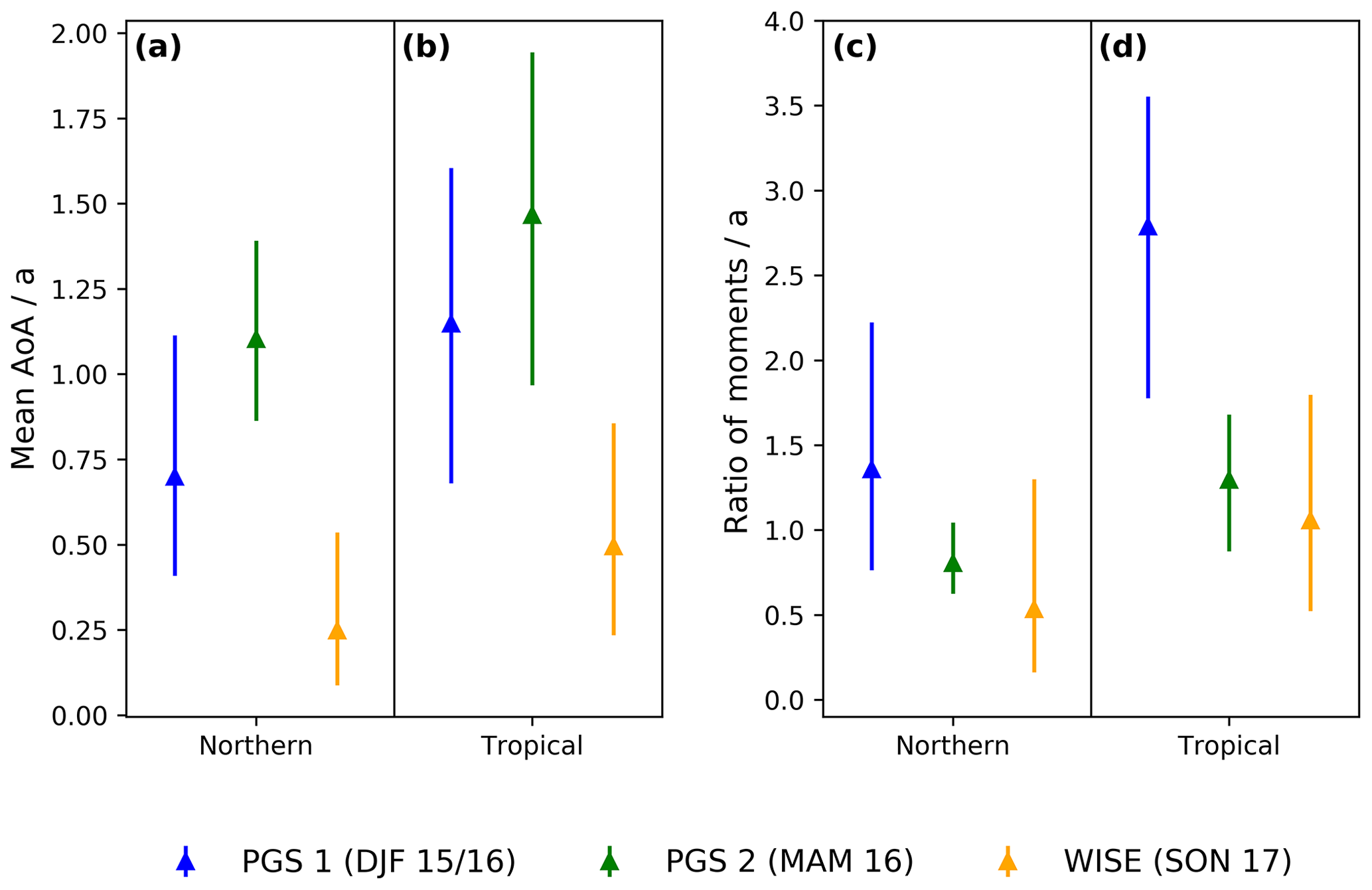
Figure 8Campaign-averaged mean AoA (a, b) and ratio of moments (c, d) derived from inverse age spectra for PGS phase 1 (blue), phase 2 (green), and WISE (orange). Data in (a) and (c) refer to the northern hemispheric tropopause section, while data in (b) and (d) use the tropical tropopause as reference. Error bars denote the mean uncertainties from the Monte Carlo simulation (see Sect. 2.2.4).
4.3.3 Campaign-averaged ratio of moments
Multiple studies in the past focused on the derivation of age-of-air spectra and mean AoA from observations in the lower stratosphere and not only constrain the shape of the age spectrum by the inverse Gaussian function of Eq. (3) but also regard a constant ratio of variance to mean AoA. This quantity is called ratio of moments μ. For instance, Volk et al. (1997) consider a ratio of moments of 1.25±0.5 years between 60∘ N and 70∘ S up to 20 km altitude, while Engel et al. (2017) and previous assessments use 0.7 years for the NH midlatitudes up to 30 km. Those values are based on model results by Hall and Plumb (1994) and might be an underestimation, since Hauck et al. (2019) demonstrate in their model simulation that the tail of the spectrum amplifies the ratio of moments considerably. They propose a ratio of moments of 2 years in the midlatitude lower stratosphere on annual average, but they state that a seasonality in μ is present. Recently, the significant influence of the ratio of moments on the derivation of mean AoA from SF6 measurements is further evaluated by Fritsch et al. (2019).
This study provides a suitable frame to reassess the assumptions for the ratio of moments. Therefore, the campaign-averaged ratios of moments for the inverse age spectra in Fig. 7 are displayed in Fig. 8c, d. It is evident that the ratio undergoes a seasonality for the inverse spectra referring to the NH tropopause section (panel c), and the maximum and minimum are retrieved as 1.36 years in PGS phase 1 and as 0.53 years during WISE. The seasonality therefore differs slightly from that found for mean AoA. The shown quantitative range of the retrieved ratio of moments matches the applied values of Volk et al. (1997) and Engel et al. (2002) reasonably well, although a solely constant value might not fully capture seasonal variations in the age spectra. In the case of the inverse age spectra with reference to the tropical tropopause (panel d), values for the ratio of moments are found to range from a 1.06-year minimum in WISE up to a 2.79-year maximum in PGS phase 1. The seasonality pattern is again different from the corresponding mean AoA seasonality but similar to the ratio of moments derived from the age spectra with NH tropopause origin. PGS phase 1 for the tropical tropopause age spectra is the only data set where the ratio of moments cannot be found in the range of values used by Volk et al. (1997) and Engel et al. (2002).
In order to constrain matching seasonal age spectra when using the ratio of moments, a value of 0.7 years or 1.25±0.5 years might not be matching universally, since results for PGS and WISE reveal that μ presents a pronounced seasonality. The inverse method could be considered as a promising alternative as the presented results show a robust performance for NH and tropical age spectra and mean AoA on a seasonal and wider geographical scale without prior constraints to the moments of the spectra, especially as the presented results demonstrated the good performance of the method compared to previous studies on transport in the NH lowermost stratosphere. However, the statistical uncertainties remain considerably high. The following section therefore provides a summary of the results as well as a critical discussion of the method's capabilities and its limitations.
This study presents an extension and application of the inverse method by Hauck et al. (2019) to derive age spectra from trace gas mixing ratios in the lowermost stratosphere by considering entry of tropospheric air across a northern (90–30∘ N), a tropical (30∘ N–30∘ S), and a southern (30–90∘ S) tropopause section, each with a distinct age spectrum. In the first part of this study, the concept of the extended method is tested in an idealized CLaMS model simulation framework. In the second part, the extended inverse method is applied to observational data of short- and long-lived halogenated trace gases measured in the NH lower stratosphere during the research campaigns PGS and WISE of the HALO research aircraft.
The newly established origin fractions turn out to be a valuable tool to assess and quantify the importance of different regions for cross-tropopause transport on a seasonal scale. Model results indicate solidly that above 450 K the stratosphere is prevalently steered by entrainment across the tropical tropopause throughout the year. Below, transport across the NH and SH tropopause gains influence, but only for the related hemisphere as cross-hemispheric transport processes appear negligible in all seasons in the model. The maximum of entrainment across the NH tropopause section is found in general around JJA and SON. That coincides with the results of Bönisch et al. (2009), who find an enhancement of quasi-isentropic mixing across the weak NH subtropical jet stream during NH summer and fall. The maximum of intrusion in the SH midlatitudes can be detected accordingly with a shift of 6 months and reduced strength compared to the north around DJF and MAM. However, these seasonality patterns are contrary to the findings of multiple studies of seasonality using the hemispherically integrated upward mass fluxes across the tropopause that indicate a maximum in late fall (Olsen et al., 2004; Schoeberl, 2004; Škerlak et al., 2014). Our results might be an indication that the NH and SH origin fractions and age spectra in CLaMS are steered primarily by the intrusion processes across the jet stream around the subtropical border of the defined source regions. It is likely that if the boundary region is confined to higher latitudes, the seasonality of the related quantities will change as well.
The performance of the inverse method in the idealized proof of concept seems consistent, and retrieval of respective age spectra in the NH and SH midlatitudes at 370 K works soundly. On the global scale, the general agreement of inverse and pulse mean AoA proves to be robust, matching both spatially and quantitatively on annual average. The seasonal cycle of mean AoA, especially during MAM and SON in the NH lowermost stratosphere, is now correctly reproduced compared to the seasonality found in Hauck et al. (2019). The improved performance of the inversion indicates the importance of transport across the extratropical tropopause for correctly retrieved seasonal age spectra in the vicinity of the tropopause. Admittedly, some improvements are certainly attributed to the fine transit time resolution (1 month) of the pulse spectra in CLaMS. If the resolution is increased in future simulations, the agreement of spectra and mean AoA will probably further advance as well, due to fully captured first modes in the age spectra. For PGS and WISE data, the inverse method retrieves age spectra and mean AoA with meaningful quantitative range and spatial and seasonal features for both the tropical and NH tropopause regions. Retrieved mean AoA referring to the NH tropopause is lower during WISE than during PGS phase 1 and phase 2. Campaign-averaged inverse age spectra consistently display a strong entrainment of tropospheric air across the NH tropopause section in fall 2017 and with reduced strength in early winter 2015/2016. Mean AoA with origin at the tropical tropopause also shows the lowest values for WISE and again an increase between PGS phase 1 and phase 2. Campaign-averaged inverse spectra indicate a strong unexpected intrusion across the tropical tropopause prior to WISE and PGS phase 1 that might be related to entrainment around the subtropical jet stream. For a thorough assessment, the ratio of moments is presented for all campaigns as it is an important quantity for the derivation of mean AoA from SF6 and CO2 in the past (Volk et al., 1997; Engel et al., 2002). Previous studies assume a constant ratio of moments, usually between 0.7 and 1.75 years, for many spatial regions in the stratosphere. Campaign-averaged results of the inverse spectra in this study indicate that the ratio of moments shows a significant seasonality, which could be incorporated in future studies for a precise mean AoA retrieval when applying the ratio of moments to constrain the age spectrum.
Although the presented results show a robust performance of the inverse method for the application to observational data, where seasonal and structural key features of transport are well-emulated and congruent with findings of earlier studies, there are multiple critical aspects that must be recognized. Although inverted age spectra and related moments retrieved from PGS and WISE data are compared to some findings in previous studies, a thorough comparison is difficult as past studies use different reference surfaces than in this study. As comparable observationally derived mean AoA values and age spectra could become available in the future, a proper comparison with the inverse method is an important task for future studies. Moreover, inverse age spectra are restricted to the seasonal scale, and an extension to finer scales (monthly) might be useful to incorporate rapid transport processes but remains difficult due to increasing variability. As indicated, the overall uncertainty of the inverse spectra and their moments is very large, and multiple factors contribute to that highly uncertain nature. The most critical aspect is the derived effective lifetimes for the species considered in this study. Holzer and Waugh (2015) indicate that their concept is applicable to derive transit time spectra in the troposphere, but errors grow significantly for stratospheric application due to the strong chemical loss process and spatial variability of most of the trace gases. We quantify these uncertainties partly by the Monte Carlo simulation to examine a variety of initial sets of trace gases together with strong statistical errors, but it is not feasible to include all possible states in the inverse method. That implies that the provided error range should be treated as a minimum. Effective lifetimes must be considered to be a highly theoretical concept and cannot be interpreted without their associated age spectrum and mixing ratio of the trace gas. A comparison to known global or local stratospheric lifetimes is not useful since effective lifetimes describe chemistry along a pathway determined by the underlying age spectrum. For completeness, resulting effective lifetimes are shown without further discussion in Fig. S4 for the campaign-averaged inverse age spectra (Sect. 4.3.2). Future studies could reassess our results by using modeled chemical lifetimes that depend explicitly on transit time from a pulsing experiment similar to Plumb et al. (1999), but resulting age spectra will then depend strongly on the chosen model setup.
This study tries to achieve a reduction of model influence by separate consideration of tropical and NH age spectra, although some information from global atmospheric models is inevitably necessary. For a fully retrieved composite age spectrum, the origin fractions must be provided by a model. The entry mixing ratio time series for all long-lived species are primarily constructed from ALE/GAGE/AGAGE measurements and extension back to 1960 using aligned mixing ratios from the RCP data set, which might not certainly constitute a precise description. Also, the time lag from the surface to the tropopause, which is assumed to be constant, might cause inaccuracies, especially in case of the NH tropopause, since the time lag is directly taken from a CLaMS simulation. All these uncertainties are considered within the applied error of entry mixing ratios of the Monte Carlo simulation, but it is not guaranteed that they are captured to their full extent. Improvements in measurement networks and technologies in the future could provide more accurate data for the tropopause sections and lead to improved age spectra. The same applies to the measured mixing ratios during PGS and WISE. These are always processed together with their standard deviation, but variability and data quality in general are crucial factors that influence the inverted age spectra significantly and contribute to the large uncertainty range of the results. Improvements to measurement data in the future, even for single species, could lead to an enhanced performance. Finally, the inverted age spectra must be evaluated carefully if assessing seasonality in transport. Since all higher-order maxima and minima in the inverse age spectra are imposed by a scaling factor that repeats for every year of transit time, possible stronger or weaker phases of real atmospheric transport are not included in the modes. Additionally, the scaling factors are derived from integrated CLaMS output and thus particularly created for the specific tropopause sections in this study. Although the seasonality matches results in previous work quite well and indicates that the subtropical jet stream is likely a dominant source region, it is likely that the retrieved scaling factors must be changed if the boundaries of the sections are shifted. Future studies could reassess these results using model output from other model simulations or differently defined NH and SH tropopause sections. Nevertheless, our results demonstrate that with the improvements to the inverse method in this study, age spectra and mean AoA can be inferred from mixing ratio measurements of atmospheric trace gases and deliver plausible results for seasonal aspects of stratospheric transport in the NH lower stratosphere. Although results must always be seen in the light of their uncertainty range, additional information on top of mean AoA can be retrieved by inclusion of further chemically active trace gas species. This might contribute to a deepened understanding of seasonal variability for future studies.
In situ data from HALO are available via the HALO database (http://halo-db.pa.op.dlr.de, German Aerospace Center, 2020). ALE/GAGE/AGAGE and RCP mixing ratio data are available online (http://agage2.eas.gatech.edu/data_archive/, Prinn et al., 2019b and http://www.pik-potsdam.de/~mmalte/rcps/index.htm, Meinshausen et al., 2011b). CLaMS model output can be made accessible on request to the authors.
The supplement related to this article is available online at: https://doi.org/10.5194/acp-20-8763-2020-supplement.
MH wrote the manuscript, performed the data processing and evaluation, and prepared the figures for this paper. MH and AE developed the extended principle of the inverse method in close collaboration. FP and MH planned, conducted, and postprocessed the CLaMS simulations. AE, HB, PH, TK, and FP were an active part in the PGS campaign and in the evaluation of data. AE, MH, PH, TK, FP, and TJS were an active part in the WISE campaign and in the evaluation of data. All co-authors contributed to the research in this paper during many discussions.
The authors declare that they have no conflict of interest.
This work is funded by the German Research Foundation (DFG) priority program 1294 (HALO) under the project numbers EN367/14-1, HO4225/8-1, and HO4225/7-1. The authors gratefully acknowledge the computing time for the CLaMS simulations granted on the supercomputer JURECA at Jülich Supercomputing Centre (JSC) under the VSR project ID JICG11. The authors greatly acknowledge all people involved with the ALE/GAGE/AGAGE network for their persistent effort in measuring atmospheric gas constituents and for provision of their data, especially people in charge at the ALE/GAGE/AGAGE stations American Samoa (Jens Mühle, Chris Harth, Paul B. Krummel and Ray Wang) and Ragged Point (Simon O'Doherty, Dickon Young, Paul B. Krummel and Ray Wang). AGAGE is supported principally by NASA (USA) grants to MIT and SIO and also by BEIS (UK) and NOAA (USA) grants to Bristol University, CSIRO and BoM (Australia), FOEN grants to Empa (Switzerland), NILU (Norway), SNU (Korea), CMA (China), NIES (Japan), and Urbino University (Italy). Finally, the authors would like to thank all organizers and participants of the PGS and WISE campaign, which provided the frame to retrieve the necessary data for this study.
This research has been supported by the Deutsche Forschungsgemeinschaft (grant nos. EN367/14-1, HO4225/8-1, and HO4225/7-1).
This open-access publication was funded by the Goethe University Frankfurt.
This paper was edited by Martin Dameris and reviewed by Eric Ray and two anonymous referees.
Abalos, M., Legras, B., Ploeger, F., and Randel, W. J.: Evaluating the advective Brewer-Dobson circulation in three reanalyses for the period 1979–2012, J. Geophys. Res., 120, 7534–7554, https://doi.org/10.1002/2015JD023182, 2015.
Allen, D. R. and Nakamura, N.: Tracer Equivalent Latitude: A Diagnostic Tool for Isentropic Transport Studies, J. Atmos. Sci., 60, 287–304, https://doi.org/10.1175/1520-0469(2003)060<0287:TELADT>2.0.CO;2, 2003.
Andrews, A. E., Boering, K. A., Daube, B. C., Wofsy, S. C., Hintsa, E. J., Weinstock, E. M., and Bui, T. P.: Empirical age spectra for the lower tropical stratosphere from in situ observations of CO2: Implications for stratospheric transport, J. Geophys. Res., 104, 26581–26595, https://doi.org/10.1029/1999JD900150, 1999.
Appenzeller, C., Holton, J. R., and Rosenlof, K. H.: Seasonal variation of mass transport across the tropopause, J. Geophys. Res., 101, 15071–15078, https://doi.org/10.1029/96JD00821, 1996.
Austin, J. and Li, F.: On the relationship between the strength of the Brewer-Dobson circulation and the age of stratospheric air, Geophys. Res. Lett., 33, L17807, https://doi.org/10.1029/2006GL026867, 2006.
Birner, T. and Bönisch, H.: Residual circulation trajectories and transit times into the extratropical lowermost stratosphere, Atmos. Chem. Phys., 11, 817–827, https://doi.org/10.5194/acp-11-817-2011, 2011.
Bönisch, H., Engel, A., Birner, Th., Hoor, P., Tarasick, D. W., and Ray, E. A.: On the structural changes in the Brewer-Dobson circulation after 2000, Atmos. Chem. Phys., 11, 3937–3948, https://doi.org/10.5194/acp-11-3937-2011, 2011.
Bönisch, H., Engel, A., Curtius, J., Birner, Th., and Hoor, P.: Quantifying transport into the lowermost stratosphere using simultaneous in-situ measurements of SF6 and CO2, Atmos. Chem. Phys., 9, 5905–5919, https://doi.org/10.5194/acp-9-5905-2009, 2009.
Boothe, A. C. and Homeyer, C. R.: Global large-scale stratosphere–troposphere exchange in modern reanalyses, Atmos. Chem. Phys., 17, 5537–5559, https://doi.org/10.5194/acp-17-5537-2017, 2017.
Butchart, N.: The Brewer-Dobson circulation, Rev. Geophys., 52, 157–184, https://doi.org/10.1002/2013RG000448, 2014.
Carpenter, L. J. and Reimann, S.: Chapter 1: Update on Ozone-Depleting Substances (ODSs) and Other Gases of Interest to the Montreal Protocol, in: Scientific Assessment of Ozone Depletion 2014, Global Ozone Research and Monitoring Project, Global Ozone Research and Monitoring Project – Report No. 55, 55, World Meteorological Organization, Geneva, Switzerland, 21–125, 2014.
Chabrillat, S., Vigouroux, C., Christophe, Y., Engel, A., Errera, Q., Minganti, D., Monge-Sanz, B. M., Segers, A., and Mahieu, E.: Comparison of mean age of air in five reanalyses using the BASCOE transport model, Atmos. Chem. Phys., 18, 14715–14735, https://doi.org/10.5194/acp-18-14715-2018, 2018.
Dee, D. P., Uppala, S. M., Simmons, A. J., Berrisford, P., Poli, P., Kobayashi, S., Andrae, U., Balmaseda, M. A., Balsamo, G., Bauer, P., Bechtold, P., Beljaars, A. C. M., van de Berg, L., Bidlot, J., Bormann, N., Delsol, C., Dragani, R., Fuentes, M., Geer, A. J., Haimberger, L., Healy, S. B., Hersbach, H., Hólm, E. V., Isaksen, L., Kållberg, P., Köhler, M., Matricardi, M., McNally, A. P., Monge-Sanz, B. M., Morcrette, J.-J., Park, B.-K., Peubey, C., de Rosnay, P., Tavolato, C., Thépaut, J.-N., and Vitart, F.: The ERA-Interim reanalysis: configuration and performance of the data assimilation system, Q. J. Roy. Meteor. Soc., 137, 553–597, https://doi.org/10.1002/qj.828, 2011.
Diallo, M., Legras, B., and Chédin, A.: Age of stratospheric air in the ERA-Interim, Atmos. Chem. Phys., 12, 12133–12154, https://doi.org/10.5194/acp-12-12133-2012, 2012.
Ehhalt, D. H., Rohrer, F., Blake, D. R., Kinnison, D. E., and Konopka, P.: On the use of nonmethane hydrocarbons for the determination of age spectra in the lower stratosphere, J. Geophys. Res., 112, 26581, https://doi.org/10.1029/2006JD007686, 2007.
Engel, A. and Rigby, M.: chap. 1: Update on Ozone-Depleting Substances (ODSs) and Other Gases of Interest to the Montreal Protocol, in: Scientific Assessment of Ozone Depletion 2018, Global Ozone Research and Monitoring Project, Global Ozone Research and Monitoring Project – Report No. 58, 58, World Meteorological Organization, Geneva, Switzerland, 2019.
Engel, A., Strunk, M., Müller, M., Haase, H.-P., Poss, C., Levin, I., and Schmidt, U.: Temporal development of total chlorine in the high-latitude stratosphere based on reference distributions of mean age derived from CO2 and SF6, J. Geophys. Res., 107, 4483, https://doi.org/10.1029/2001JD000584, 2002.
Engel, A., Möbius, T., Bönisch, H., Schmidt, U., Heinz, R., Levin, I., Atlas, E., Aoki, S., Nakazawa, T., Sugawara, S., Moore, F., Hurst, D., Elkins, J., Schauffler, S., Andrews, A., and Boering, K.: Age of stratospheric air unchanged within uncertainties over the past 30 years, Nat. Geosci., 2, 28–31, https://doi.org/10.1038/NGEO388, 2009.
Engel, A., Bönisch, H., Ullrich, M., Sitals, R., Membrive, O., Danis, F., and Crevoisier, C.: Mean age of stratospheric air derived from AirCore observations, Atmos. Chem. Phys., 17, 6825–6838, https://doi.org/10.5194/acp-17-6825-2017, 2017.
Fritsch, F., Garny, H., Engel, A., Bönisch, H., and Eichinger, R.: Sensitivity of Age of Air Trends on the derivation method for non-linear increasing tracers, Atmos. Chem. Phys. Discuss., https://doi.org/10.5194/acp-2019-974, in review, 2019.
Fueglistaler, S., Dessler, A. E., Dunkerton, T. J., Folkins, I., Fu, Q., and Mote, P. W.: Tropical tropopause layer, Rev. Geophys., 47, RG1004, https://doi.org/10.1029/2008RG000267, 2009.
Garcia, R. R. and Randel, W. J.: Acceleration of the Brewer–Dobson Circulation due to Increases in Greenhouse Gases, J. Atmos. Sci., 65, 2731–2739, https://doi.org/10.1175/2008JAS2712.1, 2008.
Garny, H., Birner, T., Bönisch, H., and Bunzel, F.: The effects of mixing on age of air, J. Geophys. Res., 119, 7015–7034, https://doi.org/10.1002/2013JD021417, 2014.
German Aerospace Center (DLR): The High Altitude and LOng Range database (HALO-DB), DLR, available at: http://halo-db.pa.op.dlr.de, last access: 22 July 2020.
Haine, T. W. N., Zhang, H., Waugh, D. W., and Holzer, M.: On transit-time distributions in unsteady circulation models, Ocean Model., 21, 35–45, https://doi.org/10.1016/j.ocemod.2007.11.004, 2008.
Hall, T. M. and Plumb, R. A.: Age as a diagnostic of stratospheric transport, J. Geophys. Res., 99, 1059, https://doi.org/10.1029/93JD03192, 1994.
Hauck, M., Fritsch, F., Garny, H., and Engel, A.: Deriving stratospheric age of air spectra using an idealized set of chemically active trace gases, Atmos. Chem. Phys., 19, 5269–5291, https://doi.org/10.5194/acp-19-5269-2019, 2019.
Haynes, P. H., McIntyre, M. E., Shepherd, T. G., Marks, C. J., and Shine, K. P.: On the “Downward Control” of Extratropical Diabatic Circulations by Eddy-Induced Mean Zonal Forces, J. Atmos. Sci., 48, 651–678, https://doi.org/10.1175/1520-0469(1991)048<0651:OTCOED>2.0.CO;2, 1991.
Hegglin, M. I. and Shepherd, T. G.: O3-N2O correlations from the Atmospheric Chemistry Experiment: Revisiting a diagnostic of transport and chemistry in the stratosphere, J. Geophys. Res., 112, D19301, https://doi.org/10.1029/2006JD008281, 2007.
Holton, J. R., Haynes, P. H., McIntyre, M. E., Douglass, A. R., Rood, R. B., and Pfister, L.: Stratosphere-troposphere exchange, Rev. Geophys., 33, RG02097, https://doi.org/10.1029/95RG02097, 1995.
Holzer, M. and Hall, T. M.: Transit-Time and Tracer-Age Distributions in Geophysical Flows, J. Atmos. Sci., 57, 3539–3558, 2000.
Holzer, M. and Primeau, F. W.: Improved constraints on transit time distributions from argon 39: A maximum entropy approach, J. Geophys. Res., 115, C12021, https://doi.org/10.1029/2010JC006410, 2010.
Holzer, M. and Waugh, D. W.: Interhemispheric transit time distributions and path-dependent lifetimes constrained by measurements of SF 6 CFCs, and CFC replacements, Geophys. Res. Lett., 42, 4581–4589, https://doi.org/10.1002/2015GL064172, 2015.
Hoor, P., Gurk, C., Brunner, D., Hegglin, M. I., Wernli, H., and Fischer, H.: Seasonality and extent of extratropical TST derived from in-situ CO measurements during SPURT, Atmos. Chem. Phys., 4, 1427–1442, https://doi.org/10.5194/acp-4-1427-2004, 2004.
Hoor, P., Fischer, H., and Lelieveld, J.: Tropical and extratropical tropospheric air in the lowermost stratosphere over Europe: A CO-based budget, Geophys. Res. Lett., 32, L07802, https://doi.org/10.1029/2004GL022018, 2005.
Keber, T., Bönisch, H., Hartick, C., Hauck, M., Lefrancois, F., Obersteiner, F., Ringsdorf, A., Schohl, N., Schuck, T., Hossaini, R., Graf, P., Jöckel, P., and Engel, A.: Bromine from short-lived source gases in the extratropical northern hemispheric upper troposphere and lower stratosphere (UTLS), Atmos. Chem. Phys., 20, 4105–4132, https://doi.org/10.5194/acp-20-4105-2020, 2020.
Kida, H.: General Circulation of Air Parcels and Transport Characteristics Derived from a Hemispheric GCM, J. Meteorol. Soc. Jpn., 61, 510–523, https://doi.org/10.2151/jmsj1965.61.4_510, 1983.
Konopka, P.: Mixing and ozone loss in the 1999–2000 Arctic vortex: Simulations with the three-dimensional Chemical Lagrangian Model of the Stratosphere (CLaMS), J. Geophys. Res., 109, D02315, https://doi.org/10.1029/2003JD003792, 2004.
Krause, J., Hoor, P., Engel, A., Plöger, F., Grooß, J.-U., Bönisch, H., Keber, T., Sinnhuber, B.-M., Woiwode, W., and Oelhaf, H.: Mixing and ageing in the polar lower stratosphere in winter 2015–2016, Atmos. Chem. Phys., 18, 6057–6073, https://doi.org/10.5194/acp-18-6057-2018, 2018.
Kunkel, D., Hoor, P., Kaluza, T., Ungermann, J., Kluschat, B., Giez, A., Lachnitt, H.-C., Kaufmann, M., and Riese, M.: Evidence of small-scale quasi-isentropic mixing in ridges of extratropical baroclinic waves, Atmos. Chem. Phys., 19, 12607–12630, https://doi.org/10.5194/acp-19-12607-2019, 2019.
Laube, J. C., Elvidge, E. C. L., Adcock, K. E., Baier, B., Brenninkmeijer, C. A. M., Chen, H., Droste, E. S., Grooß, J.-U., Heikkinen, P., Hind, A. J., Kivi, R., Lojko, A., Montzka, S. A., Oram, D. E., Randall, S., Röckmann, T., Sturges, W. T., Sweeney, C., Thomas, M., Tuffnell, E., and Ploeger, F.: Investigating stratospheric changes between 2009 and 2018 with aircraft, AirCores, and a global model focusing on CFC-11, Atmos. Chem. Phys. Discuss., https://doi.org/10.5194/acp-2020-62, in review, 2020.
Li, F., Austin, J., and Wilson, J.: The Strength of the Brewer–Dobson Circulation in a Changing Climate: Coupled Chemistry–Climate Model Simulations, J. Climate, 21, 40–57, https://doi.org/10.1175/2007JCLI1663.1, 2008.
Li, F., Waugh, D. W., Douglass, A. R., Newman, P. A., Pawson, S., Stolarski, R. S., Strahan, S. E., and Nielsen, J. E.: Seasonal variations of stratospheric age spectra in the Goddard Earth Observing System Chemistry Climate Model (GEOSCCM), J. Geophys. Res., 117, D05134, https://doi.org/10.1029/2011JD016877, 2012.
McKenna, D. S.: A new Chemical Lagrangian Model of the Stratosphere (CLaMS) 1. Formulation of advection and mixing, J. Geophys. Res., 107, 1435, https://doi.org/10.1029/2000JD000114, 2002a.
McKenna, D. S.: A new Chemical Lagrangian Model of the Stratosphere (CLaMS) 2. Formulation of chemistry scheme and initialization, J. Geophys. Res., 107, 4256, https://doi.org/10.1029/2000JD000113, 2002b.
Meinshausen, M., Smith, S. J., Calvin, K., Daniel, J. S., Kainuma, M. L. T., Lamarque, J.-F., Matsumoto, K., Montzka, S. A., Raper, S. C. B., Riahi, K., Thomson, A., Velders, G. J. M., and van Vuuren, D. P. P.: The RCP greenhouse gas concentrations and their extensions from 1765 to 2300, Climatic Change, 109, 213–241, https://doi.org/10.1007/s10584-011-0156-z, 2011a.
Meinshausen, M., S. J. Smith, K. V. Calvin, J. S. Daniel, M. L. T. Kainuma, J.-F. Lamarque, K. Matsumoto, S. A. Montzka, S. C. B. Raper, K. Riahi, A. M. Thomson; G. J. M. Velders and D. van Vuuren: The Representative Concentration Pathways (RCP) Greenhouse Gas Data, Potsdam Institute for Climate Impact Research (PIK), available at: http://www.pik-potsdam.de/~mmalte/rcps/index.htm (last access: 22 July 2020), 2011b.
Morley, S. K., Brito, T. V., and Welling, D. T.: Measures of Model Performance Based On the Log Accuracy Ratio, Space Weather, 16, 69–88, https://doi.org/10.1002/2017SW001669, 2018.
Müller, S., Hoor, P., Berkes, F., Bozem, H., Klingebiel, M., Reutter, P., Smit, H. G. J., Wendisch, M., Spichtinger, P., and Borrmann, S.: In situ detection of stratosphere-troposphere exchange of cirrus particles in the midlatitudes, Geophys. Res. Lett., 42, 949–955, https://doi.org/10.1002/2014GL062556, 2015.
Neu, J. L. and Plumb, R. A.: Age of air in a “leaky pipe” model of stratospheric transport, J. Geophys. Res., 104, 19243–19255, https://doi.org/10.1029/1999JD900251, 1999.
Oberländer-Hayn, S., Meul, S., Langematz, U., Abalichin, J., and Haenel, F.: A chemistry-climate model study of past changes in the Brewer-Dobson circulation, J. Geophys. Res., 120, 6742–6757, https://doi.org/10.1002/2014JD022843, 2015.
Oberländer-Hayn, S., Gerber, E. P., Abalichin, J., Akiyoshi, H., Kerschbaumer, A., Kubin, A., Kunze, M., Langematz, U., Meul, S., Michou, M., Morgenstern, O., and Oman, L. D.: Is the Brewer-Dobson circulation increasing or moving upward?, Geophys. Res. Lett., 43, 1772–1779, https://doi.org/10.1002/2015GL067545, 2016.
Oelhaf, H., Sinnhuber, B.-M., Woiwode, W., Bönisch, H., Bozem, H., Engel, A., Fix, A., Friedl-Vallon, F., Grooß, J.-U., Hoor, P., Johansson, S., Jurkat-Witschas, T., Kaufmann, S., Krämer, M., Krause, J., Kretschmer, E., Lörks, D., Marsing, A., Orphal, J., Pfeilsticker, K., Pitts, M., Poole, L., Preusse, P., Rapp, M., Riese, M., Rolf, C., Ungermann, J., Voigt, C., Volk, C. M., Wirth, M., Zahn, A., and Ziereis, H.: POLSTRACC: Airborne Experiment for Studying the Polar Stratosphere in a Changing Climate with the High Altitude and Long Range Research Aircraft (HALO), B. Am. Meteorol. Soc., 100, 2634–2664, https://doi.org/10.1175/BAMS-D-18-0181.1, 2019.
Olsen, M. A., Schoeberl, M. R., and Douglass, A. R.: Stratosphere-troposphere exchange of mass and ozone, J. Geophys. Res., 109, 15071, https://doi.org/10.1029/2004JD005186, 2004.
Ploeger, F. and Birner, T.: Seasonal and inter-annual variability of lower stratospheric age of air spectra, Atmos. Chem. Phys., 16, 10195–10213, https://doi.org/10.5194/acp-16-10195-2016, 2016.
Ploeger, F., Legras, B., Charlesworth, E., Yan, X., Diallo, M., Konopka, P., Birner, T., Tao, M., Engel, A., and Riese, M.: How robust are stratospheric age of air trends from different reanalyses?, Atmos. Chem. Phys., 19, 6085–6105, https://doi.org/10.5194/acp-19-6085-2019, 2019.
Plumb, I. C., Vohralik, P. F., and Ryan, K. R.: Normalization of correlations for atmospheric species with chemical loss, J. Geophys. Res., 104, 11723–11732, https://doi.org/10.1029/1999JD900014, 1999.
Plumb, R. A.: Stratospheric Transport, J. Meteorol. Soc. Jpn., 80, 793–809, https://doi.org/10.2151/jmsj.80.793, 2002.
Podglajen, A. and Ploeger, F.: Retrieving the age of air spectrum from tracers: principle and method, Atmos. Chem. Phys., 19, 1767–1783, https://doi.org/10.5194/acp-19-1767-2019, 2019.
Pommrich, R., Müller, R., Grooß, J.-U., Konopka, P., Ploeger, F., Vogel, B., Tao, M., Hoppe, C. M., Günther, G., Spelten, N., Hoffmann, L., Pumphrey, H.-C., Viciani, S., D'Amato, F., Volk, C. M., Hoor, P., Schlager, H., and Riese, M.: Tropical troposphere to stratosphere transport of carbon monoxide and long-lived trace species in the Chemical Lagrangian Model of the Stratosphere (CLaMS), Geosci. Model Dev., 7, 2895–2916, https://doi.org/10.5194/gmd-7-2895-2014, 2014.
Prinn, R. G., Weiss, R. F., Arduini, J., Arnold, T., DeWitt, H. L., Fraser, P. J., Ganesan, A. L., Gasore, J., Harth, C. M., Hermansen, O., Kim, J., Krummel, P. B., Li, S., Loh, Z. M., Lunder, C. R., Maione, M., Manning, A. J., Miller, B. R., Mitrevski, B., Mühle, J., O'Doherty, S., Park, S., Reimann, S., Rigby, M., Saito, T., Salameh, P. K., Schmidt, R., Simmonds, P. G., Steele, L. P., Vollmer, M. K., Wang, R. H., Yao, B., Yokouchi, Y., Young, D., and Zhou, L.: History of chemically and radiatively important atmospheric gases from the Advanced Global Atmospheric Gases Experiment (AGAGE), Earth Syst. Sci. Data, 10, 985–1018, https://doi.org/10.5194/essd-10-985-2018, 2018.
Prinn, R. G., Weiss, R. F., Arduini, J., Arnold, T., Fraser, P. J., Ganesan, A. L., Gasore, J., Harth, C. M., Hermansen, O., Kim, J., Krummel, P. B., Li, S., Loh, Z. M., Lunder, C. R., Maione, M., Manning, A. J., Miller, B. R., Mitrevski, B., Mühle, J., O'Doherty, S., Park, S., Reimann, S., Rigby, M., Salameh, P. K., Schmidt, R., Simmonds, P. G., Steele, L. P., Vollmer, M. K., Wang, R. H., and Young, D.: The ALE/GAGE/AGAGE Network (DB1001), OSTI.GOV, United States, https://doi.org/10.3334/CDIAC/ATG.DB1001, 2019a.
Prinn, R. G., Weiss, R. F., Arduini, J., Arnold, T., Fraser, P. J., Ganesan, A. L., Gasore, J., Harth, C. M., Hermansen, O., Kim, J., Krummel, P. B., Li, S., Loh, Z. M., Lunder, C. R., Maione, M., Manning, A. J., Miller, B. R., Mitrevski, B., Mühle, J., O'Doherty, S., Park, S., Reimann, S., Rigby, M., Salameh, P. K., Schmidt, R., Simmonds, P. G., Steele, L. P., Vollmer, M. K., Wang, R. H., and Young, D.: The ALE/GAGE/AGAGE Data Base, AGAGE, available at: http://agage2.eas.gatech.edu/data_archive/ (last access: 22 July 2020), 2019b.
Ray, E. A., Moore, F. L., Rosenlof, K. H., Davis, S. M., Sweeney, C., Tans, P., Wang, T., Elkins, J. W., Bönisch, H., Engel, A., Sugawara, S., Nakazawa, T., and Aoki, S.: Improving stratospheric transport trend analysis based on SF6 and CO2 measurements, J. Geophys. Res., 119, 14110–14128, https://doi.org/10.1002/2014JD021802, 2014.
Ray, E. A., Moore, F. L., Elkins, J. W., Rosenlof, K. H., Laube, J. C., Röckmann, T., Marsh, D. R., and Andrews, A. E.: Quantification of the SF6 lifetime based on mesospheric loss measured in the stratospheric polar vortex, J. Geophys. Res., 122, 4626–4638, https://doi.org/10.1002/2016JD026198, 2017.
Reithmeier, C., Sausen, R., and Grewe, V.: Investigating lower stratospheric model transport: Lagrangian calculations of mean age and age spectra in the GCM ECHAM4, Clim. Dynam., 30, 225–238, https://doi.org/10.1007/s00382-007-0294-1, 2008.
Rosenlof, K. H.: Seasonal cycle of the residual mean meridional circulation in the stratosphere, J. Geophys. Res., 100, 5173, https://doi.org/10.1029/94JD03122, 1995.
Rosenlof, K. H. and Holton, J. R.: Estimates of the stratospheric residual circulation using the downward control principle, J. Geophys. Res., 98, 10465, https://doi.org/10.1029/93JD00392, 1993.
Schiller, C. L., Bozem, H., Gurk, C., Parchatka, U., Königstedt, R., Harris, G. W., Lelieveld, J., and Fischer, H.: Applications of quantum cascade lasers for sensitive trace gas measurements of CO, CH4, N2O and HCHO, Appl. Phys. B, 92, 419–430, https://doi.org/10.1007/s00340-008-3125-0, 2008.
Schoeberl, M. R., Sparling, L. C., Jackman, C. H., and Fleming, E. L.: A Lagrangian view of stratospheric trace gas distributions, J. Geophys. Res., 105, 1537–1552, https://doi.org/10.1029/1999JD900787, 2000.
Schoeberl, M. R.: Extratropical stratosphere-troposphere mass exchange, J. Geophys. Res., 109, D13303, https://doi.org/10.1029/2004JD004525, 2004.
Schoeberl, M. R., Douglass, A. R., Polansky, B., Boone, C., Walker, K. A., and Bernath, P.: Estimation of stratospheric age spectrum from chemical tracers, J. Geophys. Res., 110, 32295, https://doi.org/10.1029/2005JD006125, 2005.
Shepherd, T. G.: Transport in the Middle Atmosphere, J. Meteorol. Soc. J., 85, 165–191, https://doi.org/10.2151/jmsj.85B.165, 2007.
Shepherd, T. G. and McLandress, C.: A Robust Mechanism for Strengthening of the Brewer–Dobson Circulation in Response to Climate Change: Critical-Layer Control of Subtropical Wave Breaking, J. Atmos. Sci., 68, 784–797, https://doi.org/10.1175/2010JAS3608.1, 2011.
Škerlak, B., Sprenger, M., and Wernli, H.: A global climatology of stratosphere–troposphere exchange using the ERA-Interim data set from 1979 to 2011, Atmos. Chem. Phys., 14, 913–937, https://doi.org/10.5194/acp-14-913-2014, 2014.
Solomon, S., Rosenlof, K. H., Portmann, R. W., Daniel, J. S., Davis, S. M., Sanford, T. J., and Plattner, G.-K.: Contributions of stratospheric water vapor to decadal changes in the rate of global warming, Science, 327, 1219–1223, https://doi.org/10.1126/science.1182488, 2010.
SPARC: SPARC Report on the Lifetimes of Stratospheric Ozone-Depleting Substances, Their Replacements, and Related Species, edited by: Ko, M. K. W., Newman, P. A., Reimann, S., and Strahan, S. E., SPARC Report No. 6, WCRP-15/2013, available at: https://www.sparc-climate.org/publications/sparc-reports/sparc-report-no-6/ (last access: 16 July 2020), 2013
Stiller, G. P., Fierli, F., Ploeger, F., Cagnazzo, C., Funke, B., Haenel, F. J., Reddmann, T., Riese, M., and von Clarmann, T.: Shift of subtropical transport barriers explains observed hemispheric asymmetry of decadal trends of age of air, Atmos. Chem. Phys., 17, 11177–11192, https://doi.org/10.5194/acp-17-11177-2017, 2017.
Vogel, B., Müller, R., Günther, G., Spang, R., Hanumanthu, S., Li, D., Riese, M., and Stiller, G. P.: Lagrangian simulations of the transport of young air masses to the top of the Asian monsoon anticyclone and into the tropical pipe, Atmos. Chem. Phys., 19, 6007–6034, https://doi.org/10.5194/acp-19-6007-2019, 2019.
Volk, C. M., Elkins, J. W., Fahey, D. W., Dutton, G. S., Gilligan, J. M., Loewenstein, M., Podolske, J. R., Chan, K. R., and Gunson, M. R.: Evaluation of source gas lifetimes from stratospheric observations, J. Geophys. Res., 102, 25543–25564, https://doi.org/10.1029/97JD02215, 1997.
Waugh, D. and Hall, T. M.: Age of stratospheric air: Theory, observations, and models, Rev. Geophys., 40, 4483, https://doi.org/10.1029/2000RG000101, 2002.
World Meteorological Organization: WMO WDCGG Data Summary: World Data Centre For Greenhouse Gases No. 42 – Global Atmospheric Watch Data, Volume IV – Greenhouse Gases and Other Atmospheric Gases, Japan Meteorological Agency, Japan, 2018.
Yang, H., Chen, G., Tang, Q., and Hess, P.: Quantifying isentropic stratosphere-troposphere exchange of ozone, J. Geophys. Res., 121, 3372–3387, https://doi.org/10.1002/2015JD024180, 2016.