the Creative Commons Attribution 4.0 License.
the Creative Commons Attribution 4.0 License.
 | 13 Jul 2020
Improving the prediction of an atmospheric chemistry transport model using gradient-boosted regression trees
Mathew J. Evans
Predictions from process-based models of environmental systems are biased, due to uncertainties in their inputs and parameterizations, reducing their utility. We develop a predictor for the bias in tropospheric ozone (O3, a key pollutant) calculated by an atmospheric chemistry transport model (GEOS-Chem), based on outputs from the model and observations of ozone from both the surface (EPA, EMEP, and GAW) and the ozone-sonde networks. We train a gradient-boosted decision tree algorithm (XGBoost) to predict model bias (model divided by observation), with model and observational data for 2010–2015, and then we test the approach using the years 2016–2017. We show that the bias-corrected model performs considerably better than the uncorrected model. The root-mean-square error is reduced from 16.2 to 7.5 ppb, the normalized mean bias is reduced from 0.28 to −0.04, and Pearson's R is increased from 0.48 to 0.84. Comparisons with observations from the NASA ATom flights (which were not included in the training) also show improvements but to a smaller extent, reducing the root-mean-square error (RMSE) from 12.1 to 10.5 ppb, reducing the normalized mean bias (NMB) from 0.08 to 0.06, and increasing Pearson's R from 0.76 to 0.79. We attribute the smaller improvements to the lack of routine observational constraints for much of the remote troposphere. We show that the method is robust to variations in the volume of training data, with approximately a year of data needed to produce useful performance. Data denial experiments (removing observational sites from the algorithm training) show that information from one location (for example Europe) can reduce the model bias over other locations (for example North America) which might provide insights into the processes controlling the model bias. We explore the choice of predictor (bias prediction versus direct prediction) and conclude both may have utility. We conclude that combining machine learning approaches with process-based models may provide a useful tool for improving these models.
- Article
(5420 KB) - Full-text XML
- BibTeX
- EndNote


Process-based models of the environmental system (e.g. Earth system models and their subcomponents) use quantitative understanding of physical, chemical, and biological processes to make predictions about the environmental state. These models typically solve the differential equations that represent the processes controlling the environment and are used for a range of tasks including developing new scientific understanding and environmental policies. Given uncertainties in their initial conditions, input variables, parameterizations, etc., these models show various biases which limit their usefulness for some tasks. Here we focus on predictions of the chemical composition of the atmosphere, specifically on the concentration of tropospheric ozone (O3). In this region, O3 is a climate gas (Rajendra and Myles, 2014), damages ecosystems (Emberson et al., 2018), and is thought to lead to a million deaths a year (Malley et al., 2017). The predictions of lower atmosphere O3 from process-based models are biased (Young et al., 2018), reflecting uncertainties in the emissions of compounds into the atmosphere (Rypdal and Winiwarter, 2001), the chemistry of these compounds (Newsome and Evans, 2017), and meteorology (Schuh et al., 2019). Understanding and reducing these biases is a critical scientific activity; however, the ability to improve these predictions without having to improve the model at a process level also has value. For example air quality forecasting and the quantification of the impacts air pollutants on human and ecosystem health would both benefit from improved simulations, even without process-level improvements.
Techniques used to reduce bias in air quality models include the use of ensembles (Wilczak et al., 2006) and data assimilation. Data assimilation techniques are used to incorporate observations into meteorological forecasts (Bauer et al., 2015) and some air quality models (Bocquet et al., 2015); techniques such a hybrid forecast (Kang et al., 2008; Silibello et al., 2015) or a Kalman filter (Delle Monache et al., 2006; Kang et al., 2010) have also been similarly applied.
Here we develop a method, based on machine learning approaches, to predict the bias (modelled quantity – measured quantity) in a model parameter (in this case tropospheric O3) based on information available from the model and a set of observations of the parameter. This bias predictor can then be applied more widely (in space or time) to the model output to remove the bias, bringing the model results closer to reality.
Machine learning has shown utility in the field of atmospheric science; examples include leveraging computationally burdensome short-term cloud simulations for use in climate models (Rasp et al., 2018), quantifying ocean surface CO2 distribution (Rodenbeck et al., 2015), and high-resolution mapping of precipitation from lower-resolution model output (Anderson and Lucas, 2018). More specifically to atmospheric O3, machine learning has been used for improving parameterization in climate models (Nowack et al., 2018), creating ensemble weighting for forecasts (Mallet et al., 2009) and predicting exposure during forest fire events (Watson et al., 2019). For bias correction applications, machine learning has been used to correct observational bias in dust prior to use in data assimilation (Jin et al., 2019).
Here we describe a machine learning bias correction method applied to the concentration of (O3) predicted by an atmospheric chemistry transport model. Here we describe the GEOS-Chem model used as our model (Sect. 2), the observations of O3 from four observational networks (Sect. 3), and our method (Sect. 4) to produce an algorithm to predict the bias in the model. We explore its performance (Sect. 5) and how it performs under a number of situations and analyse its resilience to a reduction in training data (Sect. 6) and training locations (Sect. 7). Finally, We explore the choice of predictor in Sect. 8 and discuss the applicability and future of such a methodology in Sect. 9.
For this analysis we use GEOS-Chem version V11-01 (Bey et al., 2001) an open-access, community, offline chemistry transport model (http://www.geos-chem.org, last access: 9 July 2020). In this proof-of-concept work, we run the model at a coarse resolution of for numerical expediency using MERRA-2 meteorology from the NASA Global Modelling and Assimilation Office (https://gmao.gsfc.nasa.gov/reanalysis/MERRA-2/, last access: 9 July 2020). The model has 47 vertical levels extending from the surface to approximately 80 km in altitude. We use the “tropchem” configuration, which has a differential equation representation of the chemistry of the troposphere, and a linearized version in the stratosphere (Eastham et al., 2014). The emissions inventories used include EDGAR (Crippa et al., 2018) and RETRO (Hu et al., 2015) inventories for global anthropogenic emissions, which are overwritten by regional inventories (NEI (USA) Travis et al., 2016; CAC (Canada) van Donkelaar et al., 2008; BRAVO (Mexico) Kuhns et al., 2005; EMEP (Europe) van Donkelaar et al., 2008; and MIX (East Asia) Li et al., 2017). GFED4 (Giglio et al., 2013) and MEGAN (Guenther et al., 2012) are used for biomass burning and biogenic emissions. Details of the other emissions used can be found online (http://wiki.seas.harvard.edu/geos-chem/index.php/HEMCO_data_directories, last access: 9 July 2020).
To produce the dataset to train the algorithm, the model is run from 1 January 2010 to 31 December 2015 outputting the local model state for each hourly observation (see Sects. 3 and 4). For the testing we run the model from 1 January 2016 to 31 December 2017 outputting the local model state hourly for every grid box within the troposphere.

Figure 1Locations of meta observations (averaged over model grid boxes) from the surface (EPA, EMEP, and GAW indicated in red), the ozone-sonde network (blue), and the ATom flights (green).
The location of all of the observations used in this study are shown in Fig. 1. Ground observations of O3 from the European Monitoring and Evaluation Programme (EMEP) (https://www.emep.int, last access: 9 July 2020), the United States Environmental Protection Agency (EPA) (https://www.epa.gov/outdoor-air-quality-data, last access: 9 July 2020), and the Global Atmospheric Watch (GAW) (https://public.wmo.int/, last access: 9 July 2020) are compiled between 2010 and 2018 (see Sofen et al., 2016, for data cleaning). Due to the coarse spatial resolution of this study (), we removed all sites flagged as “urban”, as these would not be representative at this model resolution. Similarly, all mountain sites (observations made at a pressure <850 hPa) were removed due the difficulty in representing the complex topography typical of mountain locations within the large grid boxes.
Ozone-sonde data from the World Ozone and Ultraviolet Radiation Data Centre were also used (https://woudc.org, last access: 9 July 2020). Ozone-sonde observations above 100 ppb of O3 were excluded as they are considered to be in the stratosphere (Pan et al., 2004). For both surface and sonde observations, when multiple observations were found in the same hourly model grid box (in both the horizontal and vertical) they were averaged (mean) together to create a single “meta-site”. There are 13 118 334 surface meta-site observations in the training period between 1 January 2010 and 31 December 2015 and 3 783 303 in the testing period between 1 January 2016 and 31 December 2017. There are 250 533 ozone-sonde meta-site observations in the training period and 78 451 in the testing period.
Observations of O3 from the NASA Atmospheric Tomography Mission (ATom) flights (Wofsy et al., 2018) were used as an independent testing dataset. ATom flew over the Pacific and the Atlantic from the northern mid-latitudes to the southern mid-latitudes and back from the surface to 15 km measuring the concentration of many compounds including O3 (Fig. 1). It flew for each of the four seasons between July 2016 and May 2018, but only the first three (summer, spring, and winter) are used due to availability at the time of writing. Given the oceanic nature of the flights and their sampling through the lowermost 15 km of the atmosphere, the observations collected are spatially similar to the sonde observations. As with the surface and sonde data, any O3 observations greater than 100 ppb were removed, and data were averaged onto the model grid resolution (mean) to give hourly model resolution “meta” sites. Once averaged, there are 10 518 meta observations used for the algorithm testing.
Table 1Chemical tracers and physical parameters used for training.
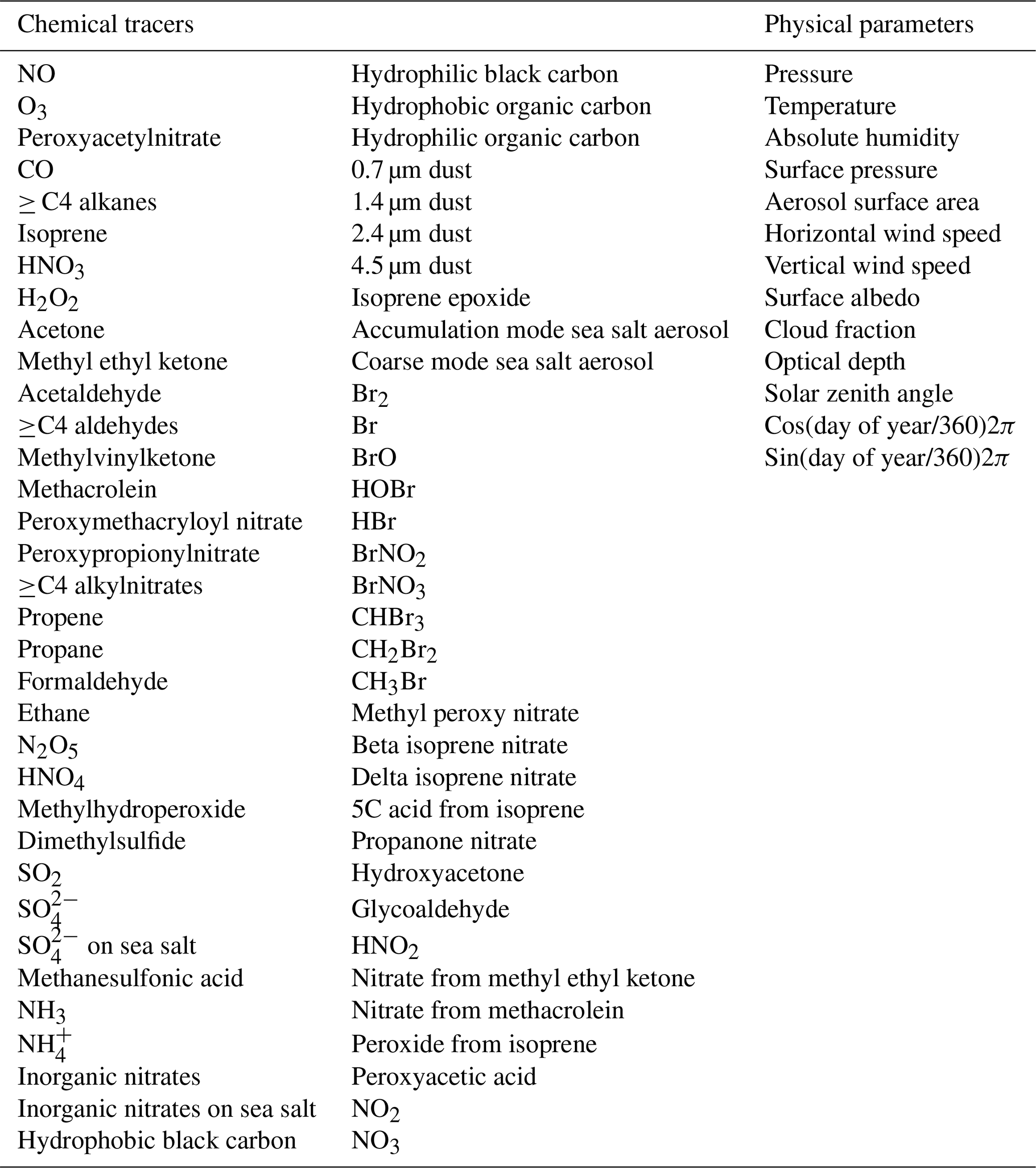
To develop a predictor for the bias in the model O3, we use the hourly observations from the surface and sondes for the training period (1 January 2010 to 31 December 2015). We run the model for the same period, outputting values of the model's local “state” at each observation location in space and time. The model local state consists of the grid box concentration of the 68 chemicals transported by the model (including O3) and 15 physical model parameters (see Table 1). The chosen parameters were thought to be the most important in determining the local conditions controlling the O3 concentration. Future work could better define the optimal set of parameters.
Once each O3 observation has a corresponding model prediction, we can develop a function to predict the model bias given the values of the model local state as input. Several potential machine learning methodologies exist for making this prediction, including neural nets (Gardner and Dorling, 1998) and decision trees (Breiman, 2001). Here we favour decision tree methods due to their increased level of explicability over neural nets (Yan et al., 2016).
As with other machine learning approaches, decision tree techniques (Blockeel and De Raedt, 1998) make a prediction for the value of a function based on a number of input variables (features) given previous values of the function and the associated values of the features. It is essentially non-linear multivariant regression. A single decision tree is a series of decision nodes that ask whether the value of a particular feature is higher than a specific value. If the value is higher, progress is made to another decision node; if it is not, progress is made to a different decision node. Ultimately, this series of decisions reaches a leaf node which gives the prediction of the function. The depth of a tree (the number of decisions needed to get to a leaf node) is an important aspect of tuning decision trees. If the tree is too shallow it will miss key relationships in the data. Conversely, if a model is too deep it will over-fit to the specific dataset and will not generalize well. The training of the system relies upon deciding which features should be used by each decision node and the specific value to be tested. The use of a single decision tree leads to over-fitting (Geurts et al., 2009), so this progressed to using random forest regression (Breiman, 2001), where a number of decision trees are constructed with differing sampling of the input data. The mean prediction of all of the decision trees (the forest) was then used as the prediction of the function. More recently, gradient-boosting regression (Friedman, 2002) relies on building a tree with a relatively shallow depth and then fitting a subsequent tree to the residuals. This is then repeated until an adequate level of complexity is reached, where the model generalizes the dataset without over-fitting.
The gradient-boosted regression technique suited our needs for a variety of reasons: it is able to capture non-linear relationships which underlie atmospheric chemistry (Krol and Poppe, 1998); the decision-tree-based machine learning technique is more interpretable than neural-net-based models (Kingsford and Salzberg, 2008), through the output of decision statistics; the technique has a relatively quick training time, allowing efficient cross validation for tuning of hyper-parameters; and it is highly scalable, meaning we are able to test on small subsets of the data before increasing to much longer training runs (Torlay et al., 2017). For the work described here we use the XGBoost (Chen and Guestrin, 2016; Frery et al., 2017) algorithm.
Hyper-parameters are parameters set before training that represent the required complexity of the system being learnt (Bergstra and Bengio, 2012). Tuning of these parameters was achieved by five k-fold cross validation whereby the training data are broken into five subsets, with the training data organized by date. The model was then trained on four of these subsets and tested on the remaining subset. Training and testing are repeated on each of the five subsets to identify the optimum hyper-parameters, attempting to balance complexity without over-fitting (Cawley and Talbot, 2010).
The key hyper-parameters tuned were the number of the trees and depth of trees. Similar results could be found with 12 to 18 layers of tree depth, with a reduction in number of trees needed at greater depth. It was found that the algorithm achieved the majority of its predictive power early on, with the bulk of the trees producing small gains in root-mean-square error. As a compromise between training time and predictive strength, 150 trees with a depth of 12 were chosen. This took 1 h to train on a 40-core CPU node, consisting of two Intel Xeon Gold 6138 CPUs. Mean-squared error was the loss function used for training.
Numerous model performance metrics are used in subsequent assessment of the model performance. The root-mean-squared error (RMSE) measures the average error in the prediction, normalized mean bias (NMB) measures the direction of the bias and normalizes the mean value, and Pearson's R correlation coefficient measures the linear relationship between the prediction and the observation.
Here y is the observed values, is the predicted values, and N is the number of samples.
Table 2Statistics for diurnal profiles at the nine selected sites for the period 1 January 2016–31 December 2017, for the base model (BM), the model with the bias correction applied (BC), the corrector trained without the nine sites (NS), and the model trained without the western hemisphere data (NWH). Statistics are described in Sect. 5.
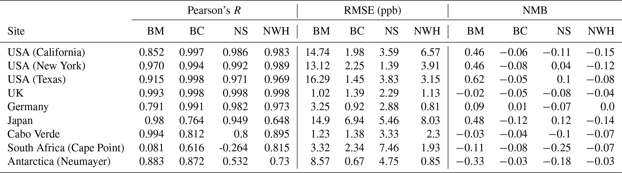
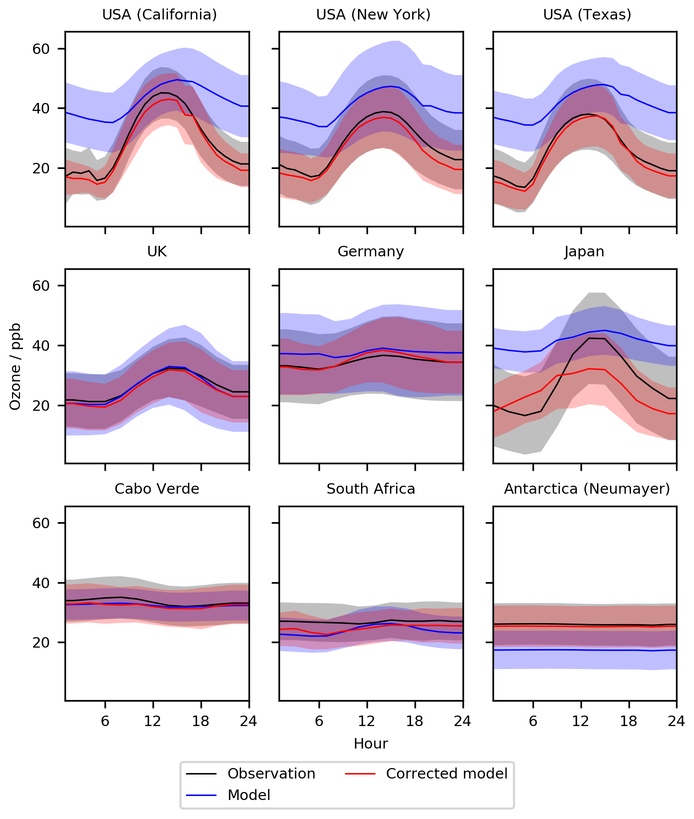
Figure 2Diurnal cycle for O3 at nine meta-sites in 2016–2017. Shown are the observations, the base model, and the model corrected with the bias predictor. The median values are shown as the continuous line and the 25th to 75th percentiles as shaded areas.
With the bias predictor now trained we can now apply it to the model output and evaluate performance. We do this for a different period (1 January 2016–31 December 2017) to that used in the training (1 January 2010–31 December 2015). We first look at the mean daily (diurnal) cycles calculated with the model for nine globally distributed sites (Fig. 2 with statistics given in Table 2). The base model (blue) shows notable differences with the observations (black) for most sites. The subtraction of the bias prediction from the base model (red) leads to an increase in the fidelity of the simulation. For the US sites, the base model overestimates at all times, consistent with previous work (Travis et al., 2016), with the largest biases occurring during the night. The bias-corrected model now shows a diurnal cycle very similar to that observed, with R increasing from a mean of 0.92 to 1.00, RMSEs decreasing from a mean of 15.1 ppb to 1.1 ppbv, and NMB decreasing from a mean of 0.51 to −0.02. The bias correction thus successfully corrects biases seen in the mean diurnal cycle, notably the large night-time bias. Although the base model failure is less evident for the European sites (Hu et al., 2018), there are still in general small improvements with the inclusion of the bias corrector. The Japanese data show a differing pattern. Similar to the US sites, the base model overestimates the O3, generating a much smaller diurnal cycle compared to the observation. Although the bias corrector improves the mean value, it does not completely correct the diurnal cycle. We attribute this to the coastal nature of Japan. The model grid box containing the Japanese observations is mainly oceanic but the observations show a continental diurnal cycle (a marked increase in O3 during the day similar to those seen in the US). It is likely that the predicted bias is being distorted by biases at other ocean-dominated grid boxes, when in Japan's case, the O3 concentration is likely influenced by long-range transport from China. For the two clean tropical sites (Cabo Verde and Cape Point in South Africa) the base model already does a reasonable job (Sherwen et al., 2016) so the bias corrected version improves little and slightly reduces the NMB performance at Cabo Verde from 0.03 to 0.04. For the Antarctic site the large bias evident in the model (Sherwen et al., 2016) is almost completely removed by the bias corrector, but that results in a small reduction in the R value.
Table 3Statistics for seasonal profiles at the nine selected sites for the period 1 January 2016–31 December 2017, for the base model (BM), the model with the bias correction applied (BC), the corrector trained without the nine sites (NS), and the model trained without the western hemisphere data (NWH). Statistics are described in Sect. 4.
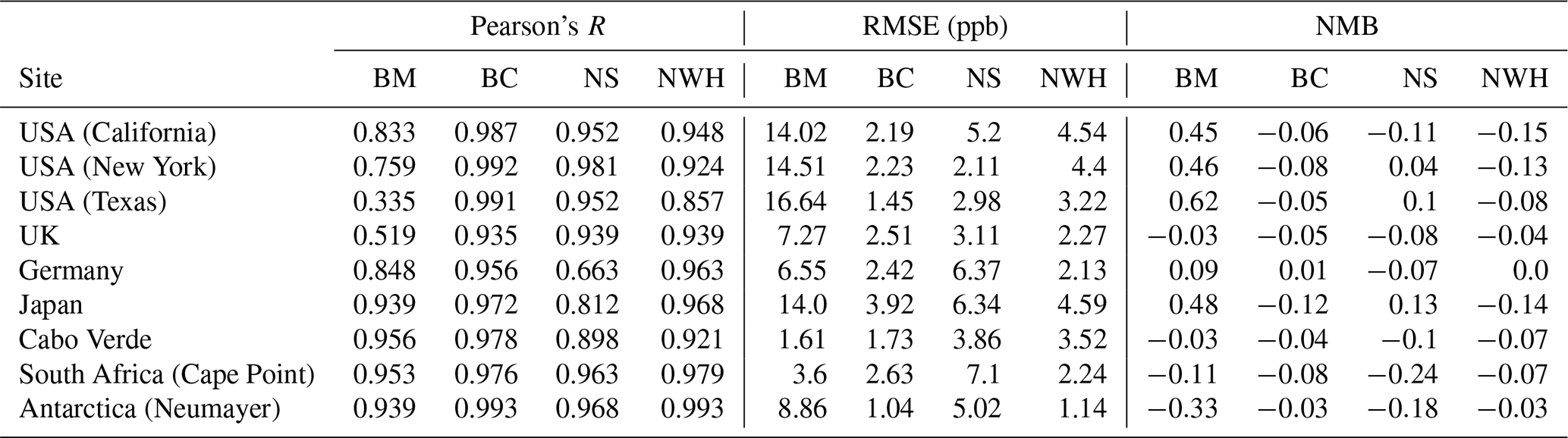

Figure 3Seasonal cycle for O3 at nine meta-sites in 2016–2017. Shown are the observations, the base model, and the model corrected with the bias predictor. The median values are shown as the continuous line and the 25th to 75th percentiles as shaded areas.
The seasonal comparison (Fig. 3 with statistics given in Table 3) shows a similar pattern. Over the polluted sites (USA, UK, Germany) biases are effectively removed. The performance for Japan is less good, with the clean tropical sites again showing only small improvements. Over Antarctica a considerable bias is removed with the application of the bias corrector. Where the performance of the model is already good, such as the RMSE at Cabo Verde or for the NMB in the UK, the inclusion of the bias correction can slightly degrade performance.
A point-by-point comparison between all of the surface data (1 January 2016–31 December 2017) and the model with and without the bias corrector is shown in Fig. 4. The bias corrector removes virtually all of the model biases (NMB) taking it from 0.29 to substantially reduces the error (RMSE) from 16.2 to 7.5 ppb, and increases the correlation (Pearson's R) from 0.48 to 0.84. Although this evaluation is for a different time period than the training dataset, it is still for the same sites. It would be preferable to use a completely different dataset to evaluate the performance of the system.
Table 4Statistical performance for the period 1 January 2016–31 December 2017 of the base model, model with a bias correction applied, and directly predicted O3 concentration. Statistics are described in Sect. 4.
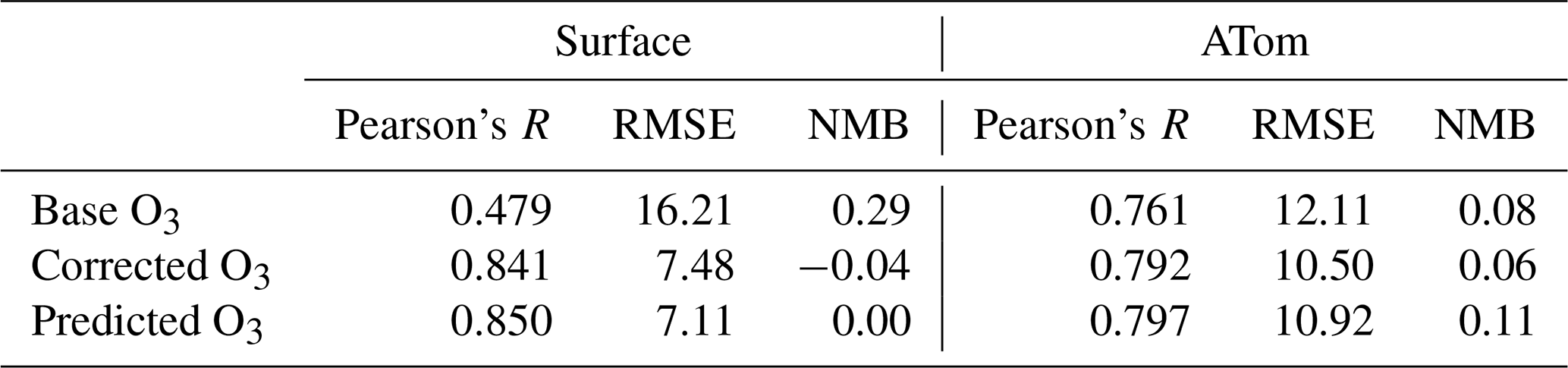

Figure 4Kernel density estimation plot of model vs. observation for all ground site observations compared to the model (a) and the corrected model (b) for 2016–2017. The dashed line indicates the 1:1 line, and the coloured line indicates the line of best fit using orthogonal regression. The plot is made up of 3 783 303 data points.
We use the ATom dataset (Sect. 3) to provide this independent evaluation. Figure 5 (with statistical data in Table 4) shows the comparison between the model prediction of the ATom observations with and without the bias corrector. Although the inclusion of the bias correction improves the performance of the model, this improvement is notably smaller than that seen for the surface data. The RMSE is reduced by only 13 % for the ATom data compared to 54 % for the surface observations. Similarly Pearson's R only marginally improves with the use of the bias corrector. Much of the improvement of the model's performance for the ATom data will be coming from the observations collected by the sonde network. There are fewer observations (40:1) collected by that network than by the surface network. Thus for the bias correction approach to work well it appears that there must be considerable volumes of observations to constrain the bias under sufficiently diverse conditions. It would appear that the sonde network may not provide that level of information to the degree that the surface network does.
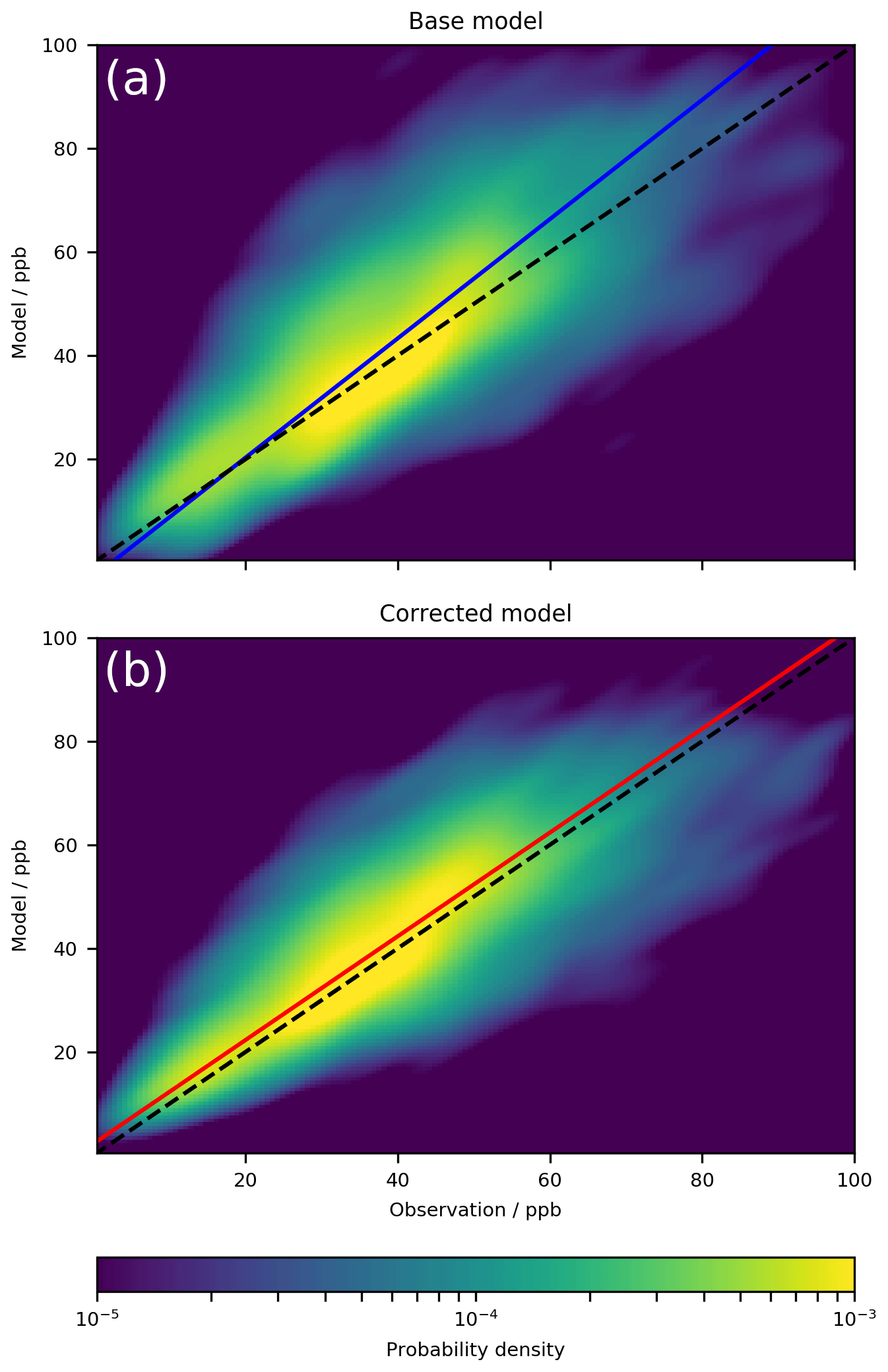
Figure 5Kernel density estimation plot of model vs. observations for all ATom summer, winter, and autumn campaign observations compared to the model (a) and the corrected model (b) for 2016–2017. The dashed line indicates the 1:1 line, and the coloured line indicates the line of best fit using orthogonal regression. The plot is made up of 10 518 data points.
Applying the bias corrector to all of the grid points within the model shows the global magnitude of the predicted bias (Fig. 6). Similar to the analysis of the nine individual sites, the base model is predicted to be biased high over much of the continental USA, with smaller biases over Europe and the tropical ocean regions. Over the southern ocean the model is predicted to be biased low. However, the bias is also predicted for regions without observations (see Fig. 1). For example, over China, the model is predicted to be biased high by ∼15 ppbv. This is higher but not dissimilar to the biases previously found for the model in China (Hu et al., 2018) which found a positive bias of 4–9 ppbv but using a different model configuration (higher resolution) and for a different model assessment (MDA8 vs. annual mean). Similar questions as to the accuracy of the prediction arise from the large biases predicted for central Africa and South America. Future evaluation of the bias correction methodology should more closely look at the impact on these regions and where possible extend the training dataset to use observations from these regions if they are available. While the algorithm is able to provide a prediction for any region, we can only have confidence in regions for which we have test data.

Figure 6Annual mean predicted bias (model – measurement) that would be applied to all grid boxes for a 1-year (2016) model simulation in three pressure ranges of the atmosphere. The >100 ppb of O3 definition of the stratosphere is used.
In the free troposphere (900 to 400 hPa) we find the model is biased low in the southern extra-tropical and polar regions and biased high in tropical regions. This matches the pattern of the bias found at 500 hPa in the ensemble comparison performed in Young et al. (2018). However, that study found that the northern extra-tropical and polar regions were biased low, whereas our results show a high bias, possibly due to a specific GEOS-Chem bias in these regions.
As we saw in the analysis of the nine individual sites, much of the improvement observed was due to the changes in the diurnal cycle. Figure 7 shows the global annual average change in diurnal cycle caused by the bias corrector. We see that there are only positive changes, increasing the amplitude of the diurnal cycle. This is likely due to the coarse model resolution not capturing the high concentration gradients required to achieve high rates of production or titration of O3. Conversely, Fig. 8 shows that over-polluted regions' seasonal amplitude decreases, which from the nine individual sites (Fig. 3) appears to be a result of reductions in the predicted summer O3 concentration.
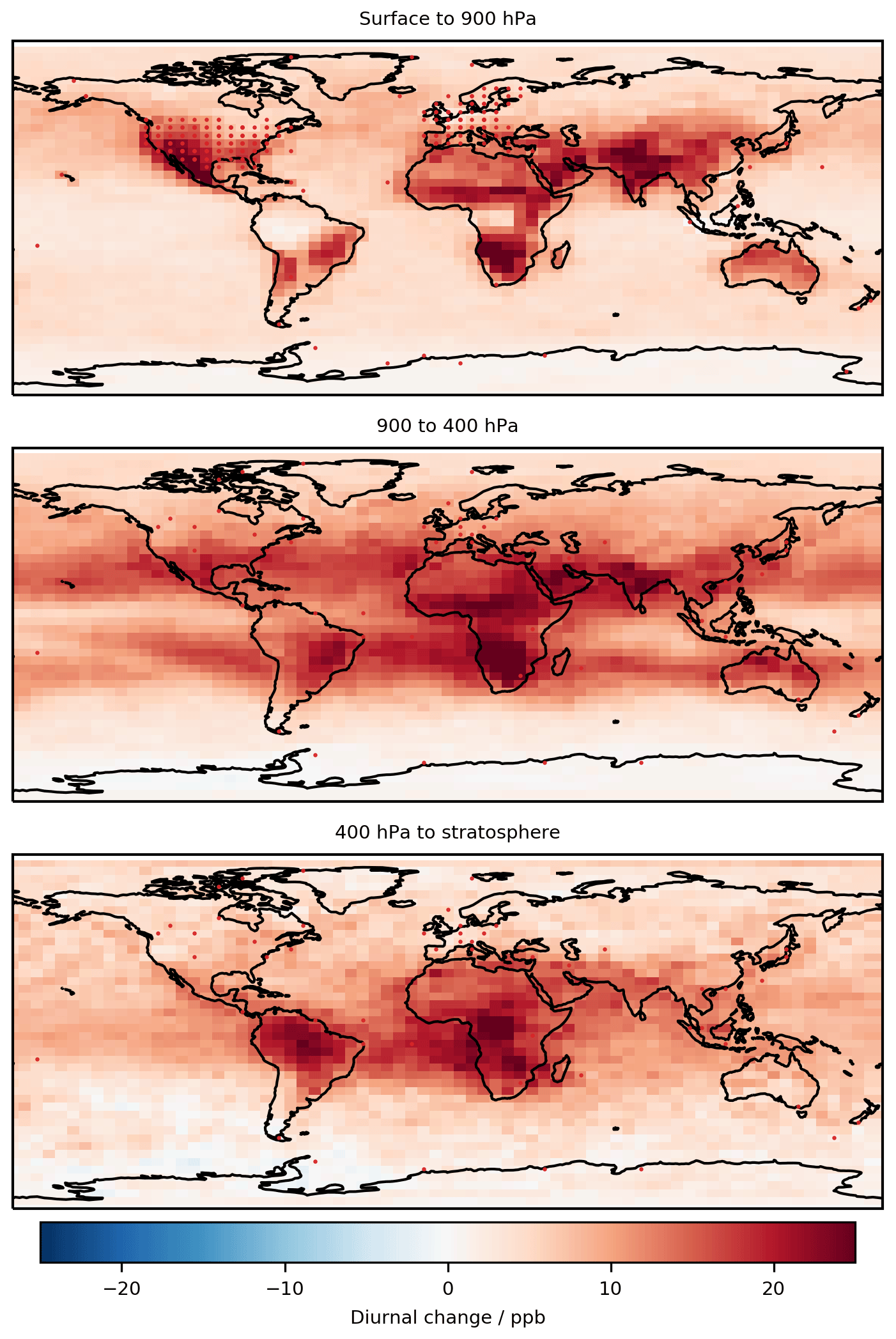
Figure 7Annual (2016) mean change (corrected model – base model) in diurnal cycle (max–min) in three pressure ranges of the atmosphere. The >100 ppb of O3 definition of the stratosphere is used.
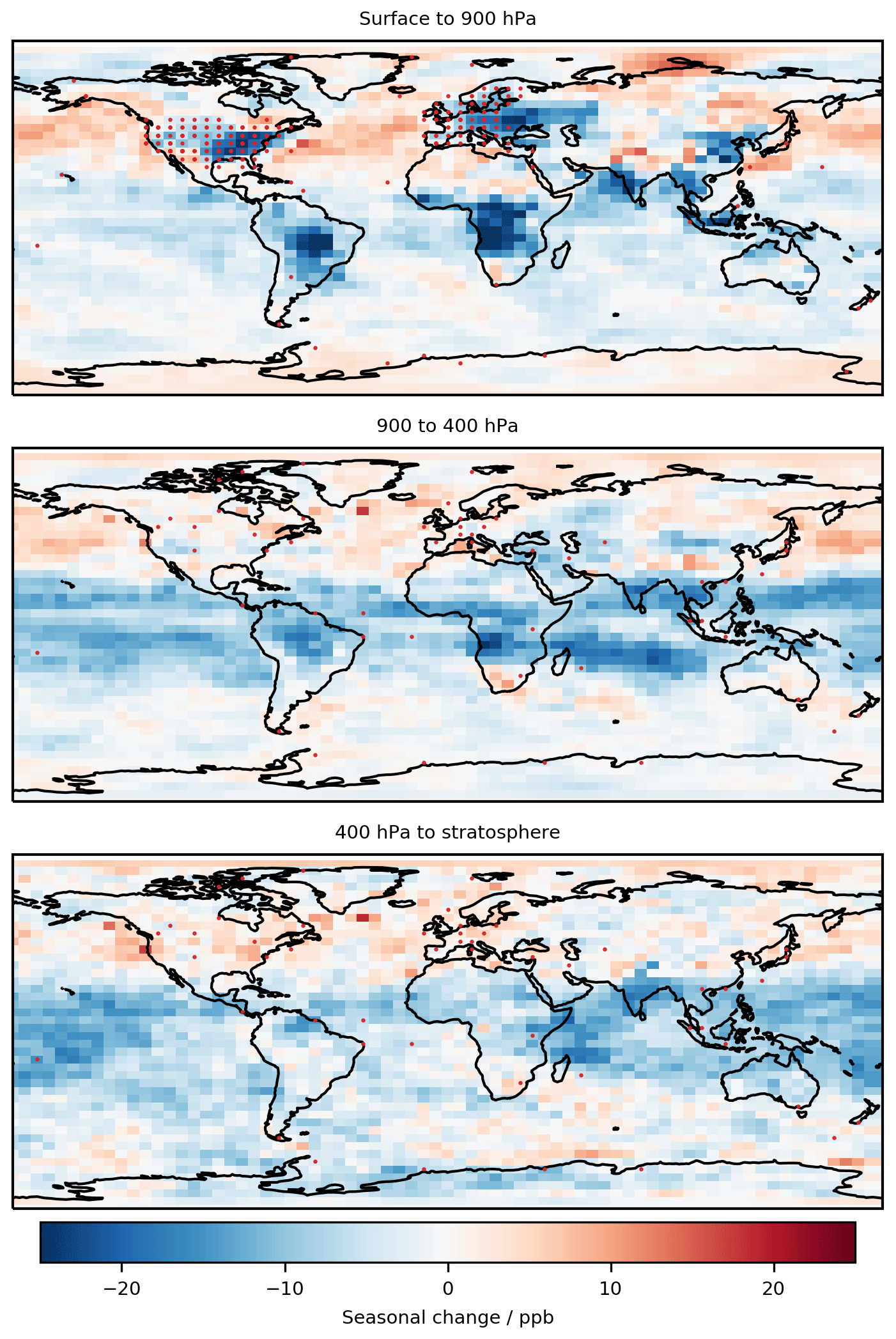
Figure 8Change (corrected model – base model) in seasonal cycle (max–min) for 2016 in three pressure ranges of the atmosphere. The >100 ppb of O3 definition of the stratosphere is used.
The gain (the loss reduction gained from splits using that feature) is shown in Fig. 9. Derivation of gain metric for XGBoost can be found in Chen and Guestrin (2016). Gain provides a diagnostic of the importance of different input variables in the decision trees used for making predictions. Surprisingly, the most important feature from this analysis is the concentration of NO3 (the nitrate radical). NO3 has a high concentration in polluted night-time environments and low concentration in clean regions or during daytime (Winer et al., 1984). The NO3 feature appears to be being used to correct the concentration of O3 in regions such as the US which are polluted and have a notably high bias at night. The next most important feature is the O3 concentration itself; this may be a result of biases arising during high- or low-O3 periods. O3 may also reflect biases in regions with very low O3 concentrations such as around Antarctica. The third most important feature is the CH2O concentration. CH2O may indicate biases over regions of high photochemical activity, as CH2O is a product of the photochemical oxidation of hydrocarbons (Wittrock et al., 2006). Future work should explore these explanatory capabilities to understand why the bias correction is performing as it is. This may also allow for a scientific understanding of why the model is biased rather than just how much the model is biased.
We have shown that the bias correction method provides an enhancement of the base-model prediction under the situations explored. We now perform some experiments with the system to explore its robustness to the size of the dataset used for training both spatially and temporally.
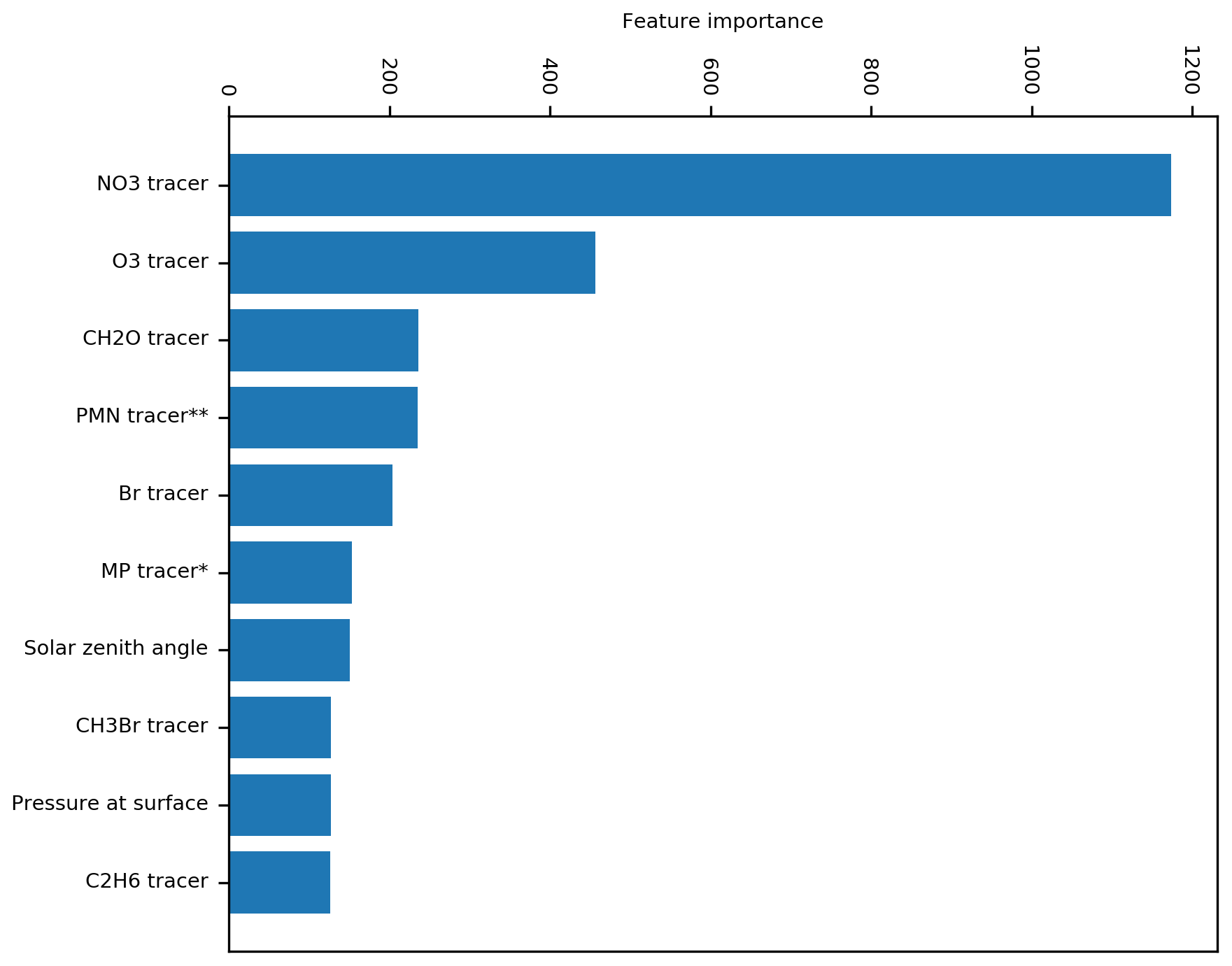
Figure 9Feature importance based on gain (the average gain across all splits the feature is used in). * Methyl-hydro-peroxide. Peroxymethacryloyl nitrate.
The bias predictor was trained using 6 years of data (2010–2015). This provides a challenge for incorporating other observational datasets. For some critical locations such as China or India the observational record is not that long, and for high-resolution model data (e.g. 12.5 km; Hu et al., 2018) managing and processing 73 parameters for 6 years could be computationally burdensome. Being able to reduce the number of years of data whilst maintaining the utility of the approach would therefore be useful. Figure 10 shows the improvement in the global performance of the model metrics (same as for Table 4) for surface O3 varying the number of months of training data used. The end of the training set was 1 January 2016 in all cases, and the starting time was pushed backwards to provide a sufficiently long training dataset. The dots in Fig. 10 represent the statistical performance of the uncorrected model. Training with only a month of data (in this case December 2015) marginally reduces the RMSE and Pearson's R. However, it causes a change in the sign of the NMB, as the model's wintertime bias is projected over the whole year. Considerable benefit arises once at least 8 months of training data have been included. Using a bias predictor trained with a year of observational data increases the performance of the base model, halving the RMSE, removing most of the NMB, and increasing Pearson's R by 60 %. Much of the variability in the power spectrum of surface O3 is captured by timescales of a year or less (Bowdalo et al., 2016); thus a timescale of a year appears to be a good balance between computational burden and utility for an operational system such as air quality forecasting. When altering the size of the training dataset we found the training time was approximately linear to the number of samples. For future high-resolution runs we may consider the use of GPUs, which have been found to substantially decrease training time (Huan et al., 2017).
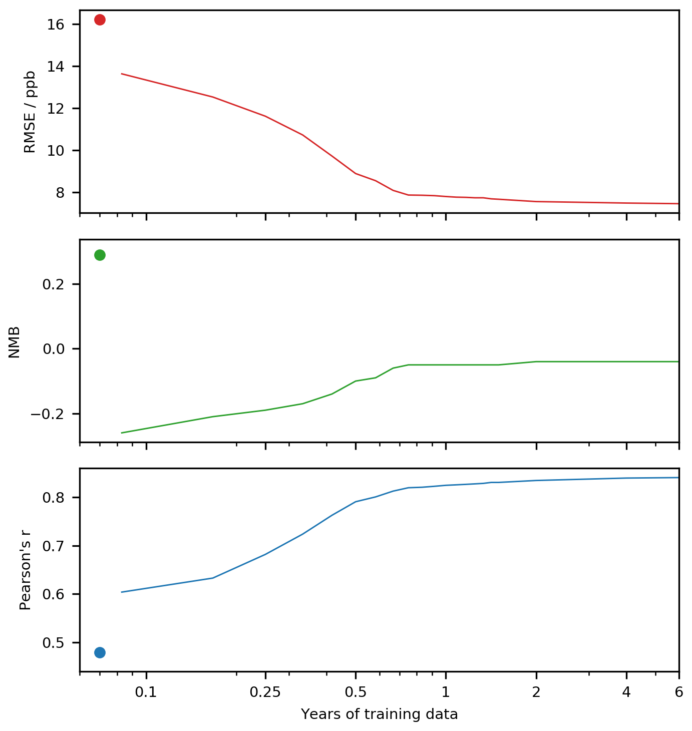
Figure 10Testing statistics with increasing length of training data. The dot represents the uncorrected model performance.

Figure 11Diurnal cycle for O3 at nine meta-sites in 2016–2017. Shown are the observations, the base model, a corrected model trained using all of the observations, and a corrected model trained with the nine sites removed. The median values are shown as the continuous line and the 25th to 75th percentiles as shaded areas.
Now we explore the impact of removing locations from the training dataset. We start by removing the data from the nine meta-sites (California, New York, Texas, UK, Germany, Japan, Cabo Verde, South Africa – Cape Point, Antarctica – Neumayer) from the algorithm training dataset (again for 2010–2015) and evaluate the bias-corrected model using this new bias predictor for these sites (again for 2016–2017) (Figs. 11 and 12). Over the USA, removing the nine observational datasets does degrade the overall model performance slightly (the green lines in Figs. 11 and 12) compared to the full training dataset (red line). It appears that the neighbouring sites are similar enough to the removed sites to provide sufficient information to almost completely correct the bias even without including the actual sites. There are different degrees of impact for the other sites. For the UK, the impact of removing the UK site from the training dataset is minimal. For Germany, the bias corrections are now larger and over-compensates for the base model during the night and in the summer months. For Japan the removal of its information provides a simulation halfway between the simulation with and without the standard bias correction. For remote sites, such as Cabo Verde and South Africa, removal makes the bias-corrected model worse than the base model. Similar to Japan, removing the Antarctic site leads to a bias correction which is between the standard bias-corrected model and the standard model. A full set of statistics for the diurnal and seasonal results can be found in Tables 2 and 3 respectively.
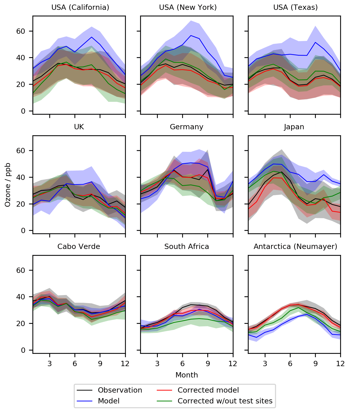
Figure 12Seasonal cycle for O3 at nine meta-sites in 2016–2017. Shown are the observations, the base model, a corrected model trained using all of the observations, and a corrected model trained with the nine sites removed. The median values are shown as the continuous line and the 25th to 75th percentiles as shaded areas.
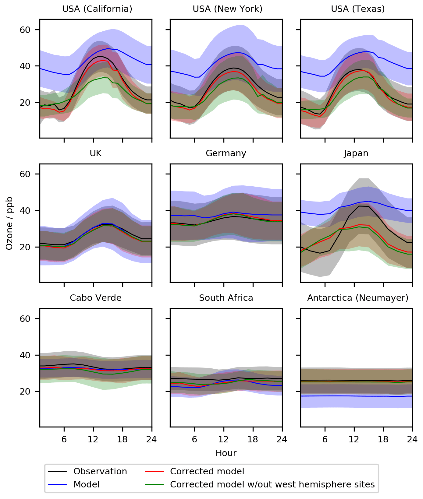
Figure 13Diurnal cycle for O3 at nine meta-sites in 2016–2017. Shown are the observations, the base model, a corrected model trained using all of the observations, and a corrected model trained with all western hemisphere (west of −20∘ E) data removed. The median values are shown as the continuous line and the 25th to 75th percentiles as shaded areas.
Much of this behaviour relates to the similarity of other sites in the training dataset to those which were removed. For sites such as the US, and to some extent Europe, removing a few sites has little influence on the bias predictor as there are a number of similar neighbouring sites which can provide that information. For other locations such as the clean Cabo Verde and South African sites there are no other similar sites. Thus removing those sites from the training dataset removes considerable amounts of information. If there are no similar sites for the bias correction to use, an inappropriate correction can be applied, which makes the simulation worse. For sites such as the Japanese and Antarctic sites there are some similar sites in the training data to provide some improvement over the base model.
Taking the data denial experiments further, we remove all observations within North and South America from the training dataset (everything between −180 and −10∘ E). Figures 13 and 14 show the impact of this on the standard nine sites. For New York and Texas the bias-corrected model performs almost as well without North and South America as it does with. The bias corrector predicts roughly the same correction for California as it does for New York and Texas, and this over-corrects daytime concentrations for California but simulates the night-time and the seasonal cycles much better than without the bias corrector. For the other six sites around the world, the influence of removing North and South America is minimal. It appears surprising that the corrections applied for North America are so good even though the North American data are not included within the training. This suggests that at least some of the reasons for the biases in the model are common between, say, North America and Europe, indicating a common source of some of the bias. This may be due to errors in the model's chemistry or meteorology, which could be global rather than local in nature.
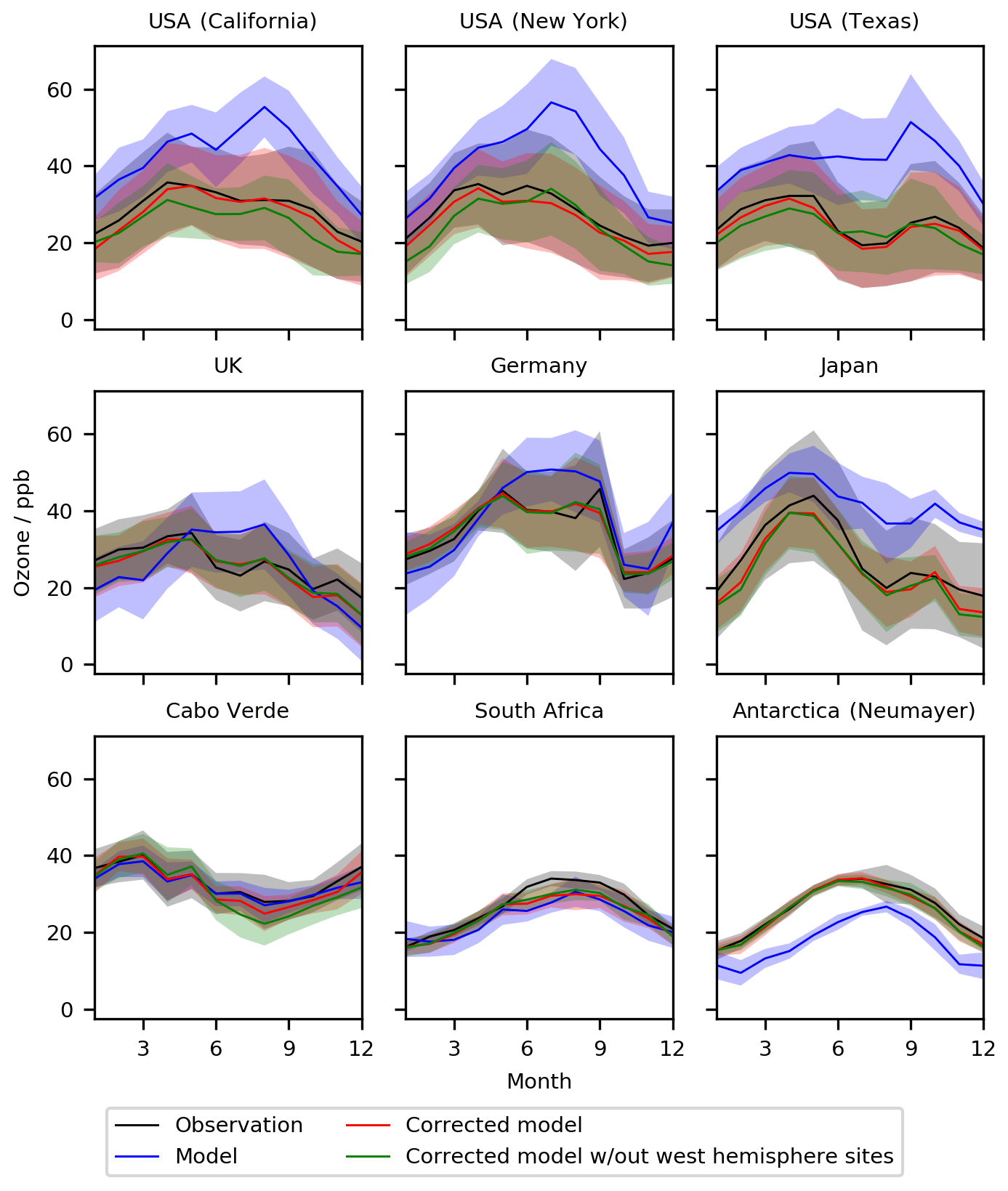
Figure 14Seasonal cycle for O3 at nine meta-sites in 2016–2017. Shown are the observations, the base model, a corrected model trained using all of the observations, and a corrected model trained with all western hemisphere (west of −20∘ E) data removed. The median values are shown as the continuous line and the 25th to 75th percentiles as shaded areas.
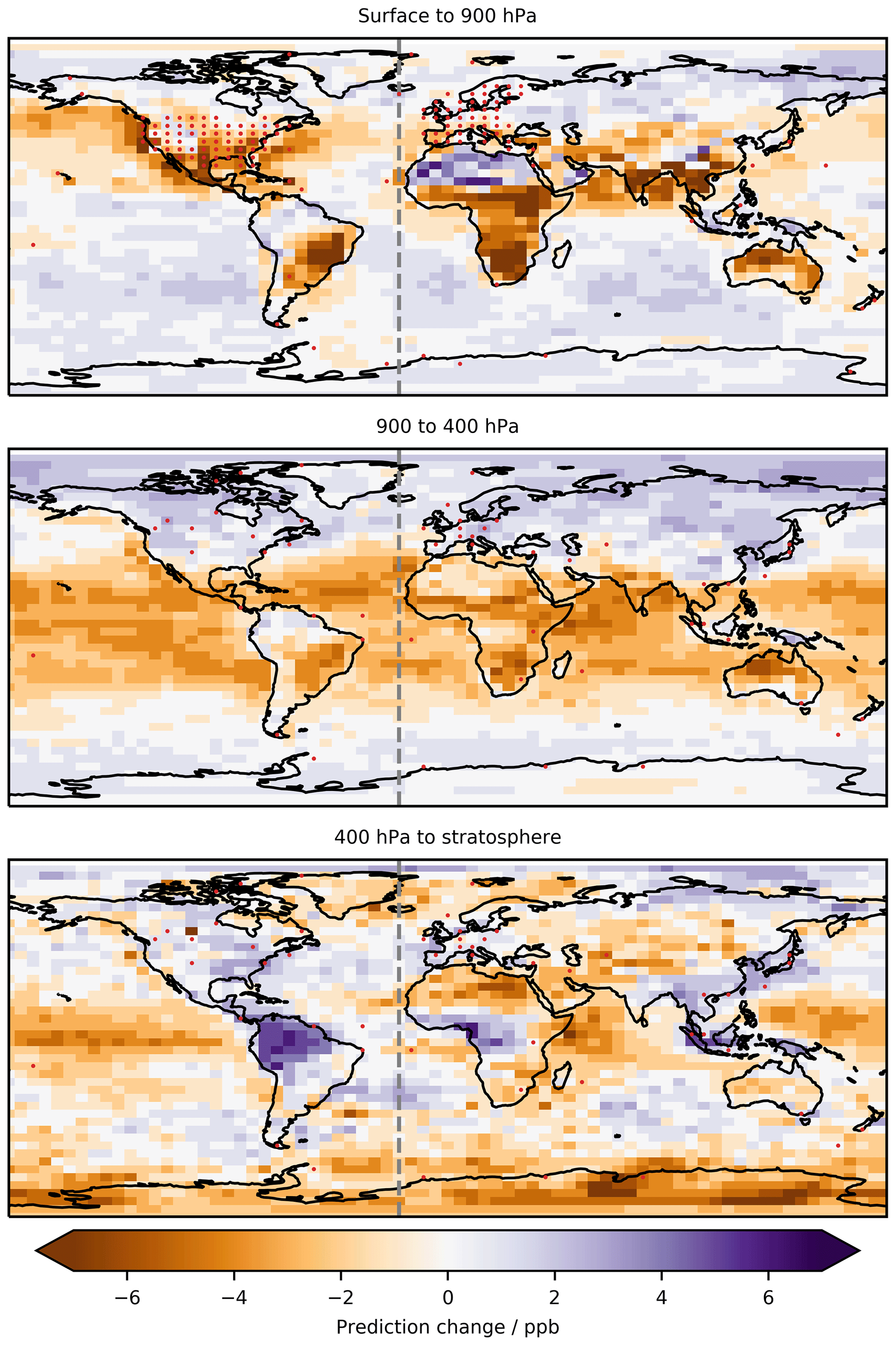
Figure 15Difference in the global mean annual surface O3 prediction between a predictor trained with western hemisphere observation data (west of −20∘ E) and a predictor trained without these data. Red dots show locations of ground sites in the surface to 900 hPa plot and sonde locations in the other two plots.
Figure 15 shows the changes in prediction that would occur globally if the western hemisphere (−180 to −10∘ E) is removed from the training data. Where there are observations in the eastern hemisphere, changes are in general small. But there are some notable changes for locations that do have observations such as in Spain. It appears the algorithm is using information from the North American observations to infer corrections for Spain. These are relatively similar locations (photolysis environment, temperatures, emissions, etc.) so the algorithm is using information from North America in the Spanish predictions. The difference in these predictions may suggest that there are different causes in the biases between the North American sites and the Spanish sites. The changes are much more profound in areas that have no observations of their own to constrain the problem. Removing the western hemisphere reduces the number of unique environments the algorithm has to learn from, resulting in substantial changes in the prediction.
It would be possible to consider other data denial experiments based on site type (rural, industrial, residential, etc.) biome, altitude, etc., which could provide information about the utility of each observation. This would likely improve with running the base model at a higher resolution than was undertaken here.
The bias correction method described here attempts to predict the bias in the model. An alternative approach would be to directly predict the O3 concentration given the values of the features including the O3 mixing ratio. An algorithm to do this given the same model local state information is trained on the standard 6 years of training data (2010–2015). Table 4 shows a statistical analysis of the performance for the model, coupled to both the bias predictor and the direct predictor. For the testing years (2016 to 2017) the direct prediction of surface O3 performs marginally better than the bias correction (RMSE of 7.1 ppb versus 7.5 ppbv, NMB of 0.00 vs. −0.04, and R of 0.85 versus 0.84).
However, for the ATom dataset, the bias predictor performs better (Table 4). We interpret this to mean that for locations where observations are included in the training (surface sites and sondes), directly predicting at locations has benefits. As XGBoost is unable to extrapolate outside the range of the observation data, direct prediction constrains to the observed O3 concentration range. While this appears beneficial in areas we have observations, at sites where no observation training data are available, it is better to use the bias correction approach as this only constrains the scale factor on the bias, not the concentration itself. Further work is necessary to advance our understanding of the form of the prediction that is necessary to best provide a useful enhancement of the system.
We have shown that the bias in the O3 concentration calculated by a chemistry transport model can be reduced through the use of a machine learning algorithm, with the results appearing robust to data denial and training length experiments. For activities such as air quality forecasting for sites with a long observational record, this appears to offer a potential route to improve fidelity of the forecasts without having to improve process-level understanding. This work offers some practical advantages over data assimilation. The observations do not necessarily need to be available in real time as the training of the bias predictor can be made using past observations and applied to a forecast without the latest observations being available. The approach may also be applied to regions where observational data are not available. Although this necessitates care, the temporary lack of availability of data is much less of a problem for this approach than for data assimilation. As forecast models are run at resolutions on the order of 1–10 km, further work will need to be done to examine the technique's performance with the added variability associated with an increase in resolution. It is possible that some mitigation may be achieved with the inclusion of additional high-resolution data, such as road usage or topological maps. The use of variables that reflect the state beyond the grid box (such as the concentration in adjacent boxes or the average of all boxes within a varying range) to provide information on upwind conditions may further improve performance.
More future work is needed to understand the approach than has been shown in this proof-of-concept work. Exploring the number and nature of the variables used would thus be advantageous. The complete set of model tracers and some physical variables were used here but their choice was somewhat arbitrary. A more systematic exploration of which variables are needed to be included is necessary. Are all the variables needed? Are important physical variables missing? Similarly, only one machine learning algorithm has been used with one set of hyper-parameters chosen. Algorithm development is occurring very quickly, and we have not explored other approaches such as neural nets that may offer improved performance. The ability to predict the bias for regions without observations is also a potentially useful tool for better constraining the global system. Observations of surface O3 exist for China (Li et al., 2019) but have not been included here for expediency. It would be scientifically interesting to see how they compare to those predicted by the bias corrector and how the bias corrector changes if they are included in the training. It seems possible that the approach developed here could be used to explore methods to extract information about why the model is biased rather than just quantifying that bias. While much of the information provided by the predictor is indicative rather than causative, coupling feature importance and data denial with domain knowledge may provide a powerful diagnostic technique for identifying the source of bias. Finally, the method could readily be extended to other model products such as PM2.5.
More generally machine learning algorithms appear to offer opportunities to understand the large, multivariate, and non-linear datasets typical of atmospheric science and the wider environmental sciences. They offer new tools to understand these scientifically interesting, computationally demanding, and socially relevant problems. However, they must also be well characterized and evaluated before they are routinely used to make the forecasts and predictions.
The GEOS-Chem model code is available from https://github.com/geoschem/geos-chem (International GEOS-Chem User Community, 2020) and the XGBoost code used is available from https://doi.org/10.1145/2939672.2939785 (Chen and Guestrin, 2016) Licensing agreements mean that we are unable to redistribute the observational dat; however they are all publicly available. The GAW O3 data are available from http://ebas.nilu.no/default.aspx (Schultz et al., 2015). The EMEP O3 data are available from http://ebas.nilu.no (Torseth et al., 2012). The EPA O3 data are available from https://aqs.epa.gov/aqsweb/airdata/download_files.html (US Environmental Protection Agency, 2020). The ozone-sonde data are available from https://doi.org/10.14287/10000008 (JMA and NASA-WFF, 2020). The ATom data are available from https://doi.org/10.3334/ornldaac/1581 (Wofsy et al., 2018).
Both authors contributed equally to the development and writing of this paper.
The authors declare that they have no conflict of interest.
This project was undertaken on the Viking Cluster, which is a high-performance computing facility provided by the University of York. We are grateful for computational support from the University of York High Performance Computing service, Viking and the Research Computing team. We also acknowledge funding from the Natural Environment Research Council (NERC) through the “Big data for atmospheric chemistry and composition: Understanding the Science (BACCHUS)” (NE/L01291X/1) grant.
We thank the numerous individuals and organizations responsible for delivering the GAW, EPA, and EMEP observations for their efforts and dedication and Tom Ryerson, Jeff Peischl, Chelsea Thompson, and Ilann Bourgeois of the NOAA Earth System Resources Laboratory's Chemical Sciences Division for their effort in collecting the ATom observations.
We thank the National Centre of Atmospheric Science for funding for Peter Ivatt through one of its Air Quality and Human Health studentships.
This research has been supported by the National Centre of Atmospheric Science (grant no. NE/L01291X/1).
This paper was edited by Chul Han Song and reviewed by two anonymous referees.
Anderson, G. J. and Lucas, D. D.: Machine Learning Predictions of a Multiresolution Climate Model Ensemble, Geophys. Res. Lett., 45, 4273–4280, https://doi.org/10.1029/2018gl077049, 2018. a
Bauer, P., Thorpe, A., and Brunet, G.: The quiet revolution of numerical weather prediction, Nature, 525, 47–55, https://doi.org/10.1038/nature14956, 2015. a
Bergstra, J. and Bengio, Y.: Random Search for Hyper-Parameter Optimization, J. Mach. Learn. Res., 13, 281–305, 2012. a
Bey, I., Jacob, D. J., Yantosca, R. M., Logan, J. A., Field, B. D., Fiore, A. M., Li, Q. B., Liu, H. G. Y., Mickley, L. J., and Schultz, M. G.: Global modeling of tropospheric chemistry with assimilated meteorology: Model description and evaluation, J. Geophys. Res.-Atmos., 106, 23073–23095, https://doi.org/10.1029/2001jd000807, 2001. a
Blockeel, H. and De Raedt, L.: Top-down induction of first-order logical decision trees, Artificial Intelligence, 101, 285–297, https://doi.org/10.1016/s0004-3702(98)00034-4, 1998. a
Bocquet, M., Elbern, H., Eskes, H., Hirtl, M., Žabkar, R., Carmichael, G. R., Flemming, J., Inness, A., Pagowski, M., Pérez Camaño, J. L., Saide, P. E., San Jose, R., Sofiev, M., Vira, J., Baklanov, A., Carnevale, C., Grell, G., and Seigneur, C.: Data assimilation in atmospheric chemistry models: current status and future prospects for coupled chemistry meteorology models, Atmos. Chem. Phys., 15, 5325–5358, https://doi.org/10.5194/acp-15-5325-2015, 2015. a
Bowdalo, D. R., Evans, M. J., and Sofen, E. D.: Spectral analysis of atmospheric composition: application to surface ozone model–measurement comparisons, Atmos. Chem. Phys., 16, 8295–8308, https://doi.org/10.5194/acp-16-8295-2016, 2016. a
Breiman, L.: Random forests, Mach. Learn., 45, 5–32, https://doi.org/10.1023/a:1010933404324, 2001. a, b
Cawley, G. C. and Talbot, N. L. C.: On Over-fitting in Model Selection and Subsequent Selection Bias in Performance Evaluation, J. Mach. Learn. Res., 11, 2079–2107, 2010. a
Chen, T. and Guestrin, C.: XGBoost: A Scalable Tree Boosting System, CoRR, 785–794, https://doi.org/10.1145/2939672.2939785, 2016. a, b
Crippa, M., Guizzardi, D., Muntean, M., Schaaf, E., Dentener, F., van Aardenne, J. A., Monni, S., Doering, U., Olivier, J. G. J., Pagliari, V., and Janssens-Maenhout, G.: Gridded emissions of air pollutants for the period 1970–2012 within EDGAR v4.3.2, Earth Syst. Sci. Data, 10, 1987–2013, https://doi.org/10.5194/essd-10-1987-2018, 2018. a
Delle Monache, L., Nipen, T., Deng, X. X., Zhou, Y. M., and Stull, R.: Ozone ensemble forecasts: 2. A Kalman filter predictor bias correction, J. Geophys. Res.-Atmos., 111, D05308, https://doi.org/10.1029/2005jd006311, 2006. a
Eastham, S. D., Weisenstein, D. K., and Barrett, S. R. H.: Development and evaluation of the unified tropospheric-stratospheric chemistry extension (UCX) for the global chemistry-transport model GEOS-Chem, Atmos. Environ., 89, 52–63, https://doi.org/10.1016/j.atmosenv.2014.02.001, 2014. a
Emberson, L. D., Pleijel, H., Ainsworth, E. A., van den Berg, M., Ren, W., Osborne, S., Mills, G., Pandey, D., Dentener, F., Buker, P., Ewert, F., Koeble, R., and Van Dingenen, R.: Ozone effects on crops and consideration in crop models, Eur. J. Agron., 100, 19–34, https://doi.org/10.1016/j.eja.2018.06.002, 2018. a
Frery, J., Habrard, A., Sebban, M., Caelen, O., and He-Guelton, L.: Efficient Top Rank Optimization with Gradient Boosting for Supervised Anomaly Detection, Machine Learning and Knowledge Discovery in Databases, Springer International Publishing, Pt I, 10534, 20–35, https://doi.org/10.1007/978-3-319-71249-9_2, 2017. a
Friedman, J. H.: Stochastic gradient boosting, Computational Statistics and Data Analysis, 38, 367–378, https://doi.org/10.1016/s0167-9473(01)00065-2, 2002. a
Gardner, M. W. and Dorling, S. R.: Artificial neural networks (the multilayer perceptron) – A review of applications in the atmospheric sciences, Atmos. Environ., 32, 2627–2636, https://doi.org/10.1016/s1352-2310(97)00447-0, 1998. a
Geurts, P., Irrthum, A., and Wehenkel, L.: Supervised learning with decision tree-based methods in computational and systems biology, Mol. Biosyst., 5, 1593–1605, https://doi.org/10.1039/b907946g, 2009. a
Giglio, L., Randerson, J. T., and van der Werf, G. R.: Analysis of daily, monthly, and annual burned area using the fourth-generation global fire emissions database (GFED4), J. Geophys. Res.-Biogeo., 118, 317–328, https://doi.org/10.1002/jgrg.20042, 2013. a
Guenther, A. B., Jiang, X., Heald, C. L., Sakulyanontvittaya, T., Duhl, T., Emmons, L. K., and Wang, X.: The Model of Emissions of Gases and Aerosols from Nature version 2.1 (MEGAN2.1): an extended and updated framework for modeling biogenic emissions, Geosci. Model Dev., 5, 1471–1492, https://doi.org/10.5194/gmd-5-1471-2012, 2012. a
Hu, L., Millet, D. B., Baasandorj, M., Griffis, T. J., Travis, K. R., Tessum, C. W., Marshall, J. D., Reinhart, W. F., Mikoviny, T., Muller, M., Wisthaler, A., Graus, M., Warneke, C., and de Gouw, J.: Emissions of C-6-C-8 aromatic compounds in the United States: Constraints from tall tower and aircraft measurements, J. Geophys. Res.-Atmos., 120, 826–842, https://doi.org/10.1002/2014jd022627, 2015. a
Hu, L., Keller, C. A., Long, M. S., Sherwen, T., Auer, B., Da Silva, A., Nielsen, J. E., Pawson, S., Thompson, M. A., Trayanov, A. L., Travis, K. R., Grange, S. K., Evans, M. J., and Jacob, D. J.: Global simulation of tropospheric chemistry at 12.5 km resolution: performance and evaluation of the GEOS-Chem chemical module (v10-1) within the NASA GEOS Earth system model (GEOS-5 ESM), Geosci. Model Dev., 11, 4603–4620, https://doi.org/10.5194/gmd-11-4603-2018, 2018. a, b, c
Huan, Z., Si, S., and Cho-Jui, H.: GPU-acceleration for Large-scale Tree Boosting, arXiv [preprint], arXiv:1706.08359, 26 June 2017. a
International GEOS-Chem User Community: geoschem/geos-chem: GEOS-Chem 11.1 (Version 11.1.0), available at: https://github.com/geoschem/geos-chem (last access: 9 July 2020), 2017.
Jin, J., Lin, H. X., Segers, A., Xie, Y., and Heemink, A.: Machine learning for observation bias correction with application to dust storm data assimilation, Atmos. Chem. Phys., 19, 10009–10026, https://doi.org/10.5194/acp-19-10009-2019, 2019. a
JMA and NASA-WFF: World Meteorological Organization-Global Atmosphere Watch Program (WMO-GAW), World Ozone and Ultraviolet Radiation Data Centre (WOUDC) [Data], https://doi.org/10.14287/10000001, 2020.
Kang, D., Mathur, R., and Rao, S. T.: Real-time bias-adjusted O3 and PM2.5 air quality index forecasts and their performance evaluations over the continental United States, Atmos. Environ., 44, 2203–2212, https://doi.org/10.1016/j.atmosenv.2010.03.017, 2010. a
Kang, D. W., Mathur, R., Rao, S. T., and Yu, S. C.: Bias adjustment techniques for improving ozone air quality forecasts, J. Geophys. Res.-Atmos., 113, D23308, https://doi.org/10.1029/2008jd010151, 2008. a
Kingsford, C. and Salzberg, S. L.: What are decision trees?, Nat. Biotechnol., 26, 1011–1013, https://doi.org/10.1038/nbt0908-1011, 2008. a
Krol, M. C. and Poppe, D.: Nonlinear dynamics in atmospheric chemistry rate equations, J. Atmos. Chem., 29, 1–16, https://doi.org/10.1023/a:1005843430146, 1998. a
Kuhns, H., Knipping, E. M., and Vukovich, J. M.: Development of a United States-Mexico emissions inventory for the Big Bend Regional Aerosol and Visibility Observational (BRAVO) Study, J. Air Waste Manage., 55, 677–692, https://doi.org/10.1080/10473289.2005.10464648, 2005. a
Li, K., Jacob, D. J., Liao, H., Shen, L., Zhang, Q., and Bates, K. H.: Anthropogenic drivers of 2013-2017 trends in summer surface ozone in China, P. Natl. Acad. Sci. USA, 116, 422–427, https://doi.org/10.1073/pnas.1812168116, 2019. a
Li, M., Zhang, Q., Kurokawa, J.-I., Woo, J.-H., He, K., Lu, Z., Ohara, T., Song, Y., Streets, D. G., Carmichael, G. R., Cheng, Y., Hong, C., Huo, H., Jiang, X., Kang, S., Liu, F., Su, H., and Zheng, B.: MIX: a mosaic Asian anthropogenic emission inventory under the international collaboration framework of the MICS-Asia and HTAP, Atmos. Chem. Phys., 17, 935–963, https://doi.org/10.5194/acp-17-935-2017, 2017. a
Mallet, V., Stoltz, G., and Mauricette, B.: Ozone ensemble forecast with machine learning algorithms, J. Geophys. Res.-Atmos., 114, D05307, https://doi.org/10.1029/2008jd009978, 2009. a
Malley, C. S., Henze, D. K., Kuylenstierna, J. C. I., Vallack, H. W., Davila, Y., Anenberg, S. C., Turner, M. C., and Ashmore, M. R.: Updated Global Estimates of Respiratory Mortality in Adults ≥30 Years of Age Attributable to Long-Term Ozone Exposure, Environ. Health Persp., 125, 087021, https://doi.org/10.1289/ehp1390, 2017. a
Newsome, B. and Evans, M.: Impact of uncertainties in inorganic chemical rate constants on tropospheric composition and ozone radiative forcing, Atmos. Chem. Phys., 17, 14333–14352, https://doi.org/10.5194/acp-17-14333-2017, 2017. a
Nowack, P., Braesicke, P., Haigh, J., Abraham, N. L., Pyle, J., and Voulgarakis, A.: Using machine learning to build temperature-based ozone parameterizations for climate sensitivity simulations, Environ. Res. Lett., 13, 104016, https://doi.org/10.1088/1748-9326/aae2be, 2018. a
Pan, L. L., Randel, W. J., Gary, B. L., Mahoney, M. J., and Hintsa, E. J.: Definitions and sharpness of the extratropical tropopause: A trace gas perspective, J. Geophys. Res.-Atmos., 109, D23103, https://doi.org/10.1029/2004jd004982, 2004. a
Rajendra, P. and Myles, A.: Climate Change 2014: Synthesis Report. Contribution of Working Groups I, II and III to the Fifth Assessment Report of the Intergovernmental Panel on Climate Change, Report, IPCC, 2014. a
Rasp, S., Pritchard, M. S., and Gentine, P.: Deep learning to represent subgrid processes in climate models, P. Natl. Acad. Sci. USA, 115, 9684–9689, https://doi.org/10.1073/pnas.1810286115, 2018. a
Rödenbeck, C., Bakker, D. C. E., Gruber, N., Iida, Y., Jacobson, A. R., Jones, S., Landschützer, P., Metzl, N., Nakaoka, S., Olsen, A., Park, G.-H., Peylin, P., Rodgers, K. B., Sasse, T. P., Schuster, U., Shutler, J. D., Valsala, V., Wanninkhof, R., and Zeng, J.: Data-based estimates of the ocean carbon sink variability – first results of the Surface Ocean pCO2 Mapping intercomparison (SOCOM), Biogeosciences, 12, 7251–7278, https://doi.org/10.5194/bg-12-7251-2015, 2015. a
Rypdal, K. and Winiwarter, W.: Uncertainties in greenhouse gas emission inventories – evaluation, comparability and implications, Environ. Sci. Policy, 4, 107–116, https://doi.org/10.1016/S1462-9011(00)00113-1, 2001. a
Schuh, A. E., Jacobson, A. R., Basu, S., Weir, B., Baker, D., Bowman, K., Chevallier, F., Crowell, S., Davis, K. J., Deng, F., Denning, S., Feng, L., Jones, D., Liu, J., and Palmer, P. I.: Quantifying the Impact of Atmospheric Transport Uncertainty on CO2 Surface Flux Estimates, Global Biogeochem. Cy., 33, 484–500, https://doi.org/10.1029/2018gb006086, 2019. a
Schultz, M. G., Akimoto, H., Bottenheim, J., Buchmann, B., Galbally, I. E., Gilge, S., Helmig, D., Koide, H., Lewis, A. C., Novelli, P. C., Plass-Dülmer, C., Ryerson, T. B., Steinbacher, M., Steinbrecher, R., Tarasova, O., Tørseth, K., Thouret, V., and Zellweger, C.: The Global Atmosphere Watch reactive gases measurement network, Elementa-Science of the Anthropocene 3, available at: http://ebas.nilu.no/default.aspx (last access: 9 July 2020), 2015.
Sherwen, T., Evans, M. J., Carpenter, L. J., Andrews, S. J., Lidster, R. T., Dix, B., Koenig, T. K., Sinreich, R., Ortega, I., Volkamer, R., Saiz-Lopez, A., Prados-Roman, C., Mahajan, A. S., and Ordóñez, C.: Iodine's impact on tropospheric oxidants: a global model study in GEOS-Chem, Atmos. Chem. Phys., 16, 1161–1186, https://doi.org/10.5194/acp-16-1161-2016, 2016. a, b
Silibello, C., D'Allura, A., Finardi, S., Bolignano, A., and Sozzi, R.: Application of bias adjustment techniques to improve air quality forecasts, Atmos. Pollut. Res., 6, 928–938, https://doi.org/10.1016/j.apr.2015.04.002, 2015. a
Sofen, E. D., Bowdalo, D., Evans, M. J., Apadula, F., Bonasoni, P., Cupeiro, M., Ellul, R., Galbally, I. E., Girgzdiene, R., Luppo, S., Mimouni, M., Nahas, A. C., Saliba, M., and Tørseth, K.: Gridded global surface ozone metrics for atmospheric chemistry model evaluation, Earth Syst. Sci. Data, 8, 41–59, https://doi.org/10.5194/essd-8-41-2016, 2016. a
Tørseth, K., Aas, W., Breivik, K., Fjæraa, A. M., Fiebig, M., Hjellbrekke, A. G., Lund Myhre, C., Solberg, S., and Yttri, K. E.: Introduction to the European Monitoring and Evaluation Programme (EMEP) and observed atmospheric composition change during 1972–2009, Atmos. Chem. Phys., 12, 5447–5481, https://doi.org/10.5194/acp-12-5447-2012, 2012 (data available at: http://ebas.nilu.no, last access: 9 July 2020).
Torlay, L., Perrone-Bertolotti, M., Thomas, E., and Baciu, M.: Machine learning-XGBoost analysis of language networks to classify patients with epilepsy, Brain informatics, 4, 159–169, https://doi.org/10.1007/s40708-017-0065-7, 2017. a
Travis, K. R., Jacob, D. J., Fisher, J. A., Kim, P. S., Marais, E. A., Zhu, L., Yu, K., Miller, C. C., Yantosca, R. M., Sulprizio, M. P., Thompson, A. M., Wennberg, P. O., Crounse, J. D., St. Clair, J. M., Cohen, R. C., Laughner, J. L., Dibb, J. E., Hall, S. R., Ullmann, K., Wolfe, G. M., Pollack, I. B., Peischl, J., Neuman, J. A., and Zhou, X.: Why do models overestimate surface ozone in the Southeast United States?, Atmos. Chem. Phys., 16, 13561–13577, https://doi.org/10.5194/acp-16-13561-2016, 2016. a, b
US Environmental Protection Agency: Air Quality System Data Mart, available at: https://aqs.epa.gov/aqsweb/airdata/download_files.html, last access: 9 July 2020.
van Donkelaar, A., Martin, R. V., Leaitch, W. R., Macdonald, A. M., Walker, T. W., Streets, D. G., Zhang, Q., Dunlea, E. J., Jimenez, J. L., Dibb, J. E., Huey, L. G., Weber, R., and Andreae, M. O.: Analysis of aircraft and satellite measurements from the Intercontinental Chemical Transport Experiment (INTEX-B) to quantify long-range transport of East Asian sulfur to Canada, Atmos. Chem. Phys., 8, 2999–3014, https://doi.org/10.5194/acp-8-2999-2008, 2008. a, b
Watson, G. L., Telesca, D., Reid, C. E., Pfister, G. G., and Jerrett, M.: Machine learning models accurately predict ozone exposure during wildfire events, Environ. Pollut., 254, 112792–112792, https://doi.org/10.1016/j.envpol.2019.06.088, 2019. a
Wilczak, J., McKeen, S., Djalalova, I., Grell, G., Peckham, S., Gong, W., Bouchet, V., Moffet, R., McHenry, J., McQueen, J., Lee, P., Tang, Y., and Carmichael, G. R.: Bias-corrected ensemble and probabilistic forecasts of surface ozone over eastern North America during the summer of 2004, J. Geophys. Res.-Atmos., 111, D23S28, https://doi.org/10.1029/2006jd007598, 2006. a
Winer, A. M., Atkinson, R., and Pitts, J. N.: Gaseous Nitrate Radical – Possible Nighttime Atmospheric Sink for Biogenic Organic-compounds, Science, 224, 156–159, https://doi.org/10.1126/science.224.4645.156, 1984. a
Wittrock, F., Richter, A., Oetjen, H., Burrows, J. P., Kanakidou, M., Myriokefalitakis, S., Volkamer, R., Beirle, S., Platt, U., and Wagner, T.: Simultaneous global observations of glyoxal and formaldehyde from space, Geophys. Res. Lett., 33, L16804, https://doi.org/10.1029/2006gl026310, 2006. a
Wofsy, S., Afshar, S., Allen, H., Apel, E., Asher, E., Barletta, B., Bent, J., Bian, H., Biggs, B., Blake, D., Blake, N., Bourgeois, I., Brock, C., Brune, W., Budney, J., Bui, T., Butler, A., Campuzano-jost, P., Chang, C., Chin, M., Commane, R., Correa, G., Crounse, J., Cullis, P., Daube, B., Day, D., Dean-day, J., Dibb, J., Digangi, J., Diskin, G., Dollner, M., Elkins, J., Erdesz, F., Fiore, A., Flynn, C., Froyd, K., Gesler, D., Hall, S., Hanisco, T., Hannun, R., Hills, A., Hintsa, E., Hoffman, A., Hornbrook, R., Huey, L., Hughes, S., Jimenez, J., Johnson, B., Katich, J., Keeling, R., Kim, M., Kupc, A., Lait, L., Lamarque, J., Liu, J., Mckain, K., Mclaughlin, R., Meinardi, S., Miller, D., Montzka, S., Moore, F., Morgan, E., Murphy, D., Murray, L., Nault, B., Neuman, J., Newman, P., Nicely, J., Pan, X., Paplawsky, W., Peischl, J., Prather, M., Price, D., Ray, E., Reeves, J., Richardson, M., Rollins, A., Rosenlof, K., Ryerson, T., Scheuer, E., Schill, G., Schroder, J., Schwarz, J., St.clair, J., Steenrod, S., Stephens, B., Strode, S., Sweeney, C., Tanner, D., Teng, A., Thames, A., Thompson, C., Ullmann, K., Veres, P., Vizenor, N., Wagner, N., Watt, A., Weber, R., Weinzierl, B., Wennberg, P., et al.: ATom: Merged Atmospheric Chemistry, Trace Gases, and Aerosols, ORNL DAAC, Oak Ridge, Tennessee, USA, https://doi.org/10.3334/ORNLDAAC/1581, 2018. a, b
Yan, R., Ma, Z. J., Zhao, Y., and Kokogiannakis, G.: A decision tree based data-driven diagnostic strategy for air handling units, Energ. Buildings, 133, 37–45, https://doi.org/10.1016/j.enbuild.2016.09.039, 2016. a
Young, P. J., Naik, V., Fiore, A. M., Gaudel, A., Guo, J., Lin, M. Y., Neu, J. L., Parrish, D. D., Rieder, H. E., Schnell, J. L., Tilmes, S., Wild, O., Zhang, L., Ziemke, J., Brandt, J., Delcloo, A., Doherty, R. M., Geels, C., Hegglin, M. I., Hu, L., Im, U., Kumar, R., Luhar, A., Murray, L., Plummer, D., Rodriguez, J., Saiz-Lopez, A., Schultz, M. G., Woodhouse, M. T., and Zeng, G.: Tropospheric Ozone Assessment Report: Assessment of global-scale model performance for global and regional ozone distributions, variability, and trends, Elementa-Science of the Anthropocene, 6, 10, https://doi.org/10.1525/elementa.265, 2018. a, b
- Abstract
- Introduction
- GEOS-Chem model
- Observational dataset
- Developing the bias predictor
- Application
- Size of training dataset
- Data denial
- Nature of the prediction
- Discussion
- Code and data availability
- Author contributions
- Competing interests
- Acknowledgements
- Financial support
- Review statement
- References