Technical note: Equilibrium droplet size distributions in a turbulent cloud chamber with uniform supersaturation

In a laboratory cloud chamber that is undergoing Rayleigh–Bénard convection, supersaturation is produced by isobaric mixing. When aerosols (cloud condensation nuclei) are injected into the chamber at a constant rate, and the rate of droplet activation is balanced by the rate of droplet loss, an equilibrium droplet size distribution (DSD) can be achieved. We derived analytic equilibrium DSDs and probability density functions (PDFs) of droplet radius and squared radius for conditions that could occur in such a turbulent cloud chamber when there is uniform supersaturation. We neglected the effects of droplet curvature and solute on the droplet growth rate. The loss rate due to fallout that we used assumes that (1) the droplets are well-mixed by turbulence, (2) when a droplet becomes sufficiently close to the lower boundary, the droplet's terminal velocity determines its probability of fallout per unit time, and (3) a droplet's terminal velocity follows Stokes' law (so it is proportional to its radius squared). Given the chamber height, the analytic PDF is determined by the mean supersaturation alone. From the expression for the PDF of the radius, we obtained analytic expressions for the first five moments of the radius, including moments for truncated DSDs. We used statistics from a set of measured DSDs to check for consistency with the analytic PDF. We found consistency between the theoretical and measured moments, but only when the truncation radius of the measured DSDs was taken into account. This consistency allows us to infer the mean supersaturations that would produce the measured PDFs in the absence of supersaturation fluctuations. We found that accounting for the truncation radius of the measured DSDs is particularly important when comparing the theoretical and measured relative dispersions of the droplet radius. We also included some additional quantities derived from the analytic DSD: droplet sedimentation flux, precipitation flux, and condensation rate.

1 Introduction

In a laboratory cloud chamber, such as the Π chamber at Michigan Technological University (Chang et al., 2016), it is possible to produce Rayleigh–Bénard convection by applying an unstable temperature gradient between the top and bottom water-saturated surfaces of the chamber. Supersaturation is produced by isobaric mixing within the turbulent flow. When aerosols (cloud condensation nuclei) are injected at a constant rate, an equilibrium state is achieved in which the rate of droplet activation is balanced by the rate of droplet loss. After a droplet is activated, it continues to grow by condensation until it falls out (i.e., contacts the bottom surface).

Although the resulting equilibrium droplet size distributions (DSDs) have been extensively measured in the Π chamber, and theoretical models proposed for some aspects of the DSDs (e.g., Chandrakar et al., 2016, 2017, 2018a, c; Saito et al., 2019), obtaining a complete quantitative theory for the equilibrium DSDs has been elusive. The reasons for this include the difficulty of accurately measuring supersaturation in a cloud chamber (e.g., Chandrakar et al., 2016) as well as uncertainties in our knowledge of the physical processes that determine the DSD. In particular, we do not know the relative importance of mean supersaturation and supersaturation fluctuations, nor do we have a quantitative understanding of droplet fallout.

In this study, we assume that (1) droplets grow subject to a uniform mean supersaturation, (2) the effects of droplet curvature and solute on the droplet growth rate can be neglected, and (3) droplets fall relative to the turbulent flow at their Stokes' fall speed (for example, they are not affected by turbophoresis or thermophoresis). In Sect. 1, we derive the equations which govern the evolution of the droplet radius and squared radius distributions, including the loss rate due to sedimentation. In Sect. 2, we show how the equilibrium radius distribution is realized by using a Monte Carlo method and compare the results to those that are obtained analytically in later sections. In Sect. 3, we derive the analytic equilibrium solutions for the distributions and probability density functions (PDFs) of radius and of squared radius and from these obtain expressions for the median and mode radii. In Sect. 4, we derive the first five moments of the radius from the analytic equilibrium PDFs, including moments for truncated DSDs (those with positive lower limits). In Sect. 6, we use statistics from a set of measured DSDs to check for consistency with the analytic DSD. We also demonstrate the importance of taking into account a non-zero truncation radius when comparing theoretical moments to moments from a measured but truncated DSD. In Sect. 7, we present some additional quantities derived from the analytic DSD: droplet sedimentation flux, mean and PDF of the droplet residence time, precipitation flux, and condensation rate. Finally, Sect. 8 contains the conclusions.

2 Governing equations

Our initial goal is to develop and solve the equations that govern the equilibrium droplet radius distribution under conditions that might be found in the Π chamber. Specifically, we assume that (1) droplets grow subject to a uniform mean supersaturation and (2) droplets fall relative to the turbulent flow at their Stokes' fall speed (for example, they are not affected by turbophoresis or thermophoresis).

2.1 Distribution of r

We follow the notation used in Rogers and Yau (1989). They derived the following equation (their Eq. 7.31), which governs the evolution of the droplet radius distribution, v(r,t), subject to condensation:

$$\begin{array}{}\text{(1)}& {\displaystyle \frac{\partial v\left(r\right)}{\partial t}}=-{\displaystyle \frac{\partial }{\partial r}}\left(v{\displaystyle \frac{\mathrm{d}r}{\mathrm{d}t}}\right).\end{array}$$

Here v(r) dr is the number of cloud droplets per unit mass of air with radii in the interval $(r,r+\mathrm{d}r)$. The condensational growth rate is $\mathrm{d}r/\mathrm{d}t=\mathit{\xi }/r$, where

$$\mathit{\xi }={\displaystyle \frac{S-\mathrm{1}}{F_k+F_{\mathrm{d}}}},$$

$S=e/e_{\mathrm{s}}\left(T\right)$ is the saturation ratio, e is the vapor pressure, e_s(T) is the equilibrium vapor pressure over a plane water surface at temperature T, F_k represents the thermodynamic term in the denominator that is associated with heat conduction, and F_d is the term associated with vapor diffusion (Rogers and Yau, 1989). The effects of droplet curvature and solute on droplet condensational growth are usually considered to be negligible for activated droplets (Rogers and Yau, 1989; Siewert et al., 2017). However, in cloud chambers with low mean supersaturation, and therefore large droplet residence times, curvature and solute effects might become significant (Srivastava, 1991). Nevertheless, we neglect both effects in the governing equations but briefly address the consequences of doing so in Sect. 6.2.

To generalize this to the cloud chamber in the presence of aerosol injection (which produces new droplets at a steady rate) and sedimentation (which removes droplets that fall to the bottom of the chamber), we add two terms to Eq. (1) so that it becomes

$$\begin{array}{}\text{(2)}& {\displaystyle \frac{\partial v\left(r\right)}{\partial t}}=-{\displaystyle \frac{\partial }{\partial r}}\left(\mathit{\xi }{\displaystyle \frac{v}{r}}\right)-v{\displaystyle \frac{u}{h}}+A\left(r\right),\end{array}$$

where u=k₁ r² is Stokes' law droplet terminal velocity, h is the height of the chamber, and A(r) is the rate of production of (activated) droplets from the injected aerosol.

2.2 Distribution of r²

Analogous to Eq. (1), the following equation governs the evolution of the squared radius distribution, w(s,t), subject to condensation:

$$\begin{array}{}\text{(3)}& {\displaystyle \frac{\partial w\left(s\right)}{\partial t}}=-{\displaystyle \frac{\partial }{\partial s}}\left(w{\displaystyle \frac{\mathrm{d}s}{\mathrm{d}t}}\right).\end{array}$$

Here w(s) ds is the number of cloud droplets per unit mass of air with s≡r² in the interval $(s,s+\mathrm{d}s)$. The condensational growth rate is $\mathrm{d}s/\mathrm{d}t=\mathrm{d}{r}^{\mathrm{2}}/\mathrm{d}t=\mathrm{2}\mathit{\xi }$. When this is substituted into Eq. (3), the result is

$$\begin{array}{}\text{(4)}& {\displaystyle \frac{\partial w\left(s\right)}{\partial t}}=-\mathrm{2}\mathit{\xi }{\displaystyle \frac{\partial w}{\partial s}},\end{array}$$

which has the form of the 1-D advection equation, with solution

$$\begin{array}{}\text{(5)}& w(s,t)=w_{\mathrm{0}}(s-\mathrm{2}\mathit{\xi }t),\end{array}$$

where the initial condition w₀(s) is an arbitrary function. The solution (Eq. 5) states that the initial distribution of s=r² simply translates at a rate 2ξ towards larger values of r² without any change of shape.

To generalize Eq. (4) to the cloud chamber in the presence of aerosol injection and sedimentation, we add two terms to Eq. (4) so that it becomes

$$\begin{array}{}\text{(6)}& {\displaystyle \frac{\partial w\left(s\right)}{\partial t}}=-\mathrm{2}\mathit{\xi }{\displaystyle \frac{\partial w}{\partial s}}-w{\displaystyle \frac{k_{\mathrm{1}}}{h}}s+B\left(s\right),\end{array}$$

where u=k₁s is Stokes' law droplet terminal velocity and B(s) is the rate of production of (activated) droplets from the injected aerosol.

2.3 Loss rate due to sedimentation

The probability that a droplet of radius r will fall out due to sedimentation in a small time interval Δt is $(u/h)\mathrm{\Delta }t=(k_{\mathrm{1}}{r}^{\mathrm{2}}/h)\mathrm{\Delta }t$. This can be derived as follows. We assume that the droplets are well-mixed, in which case the z coordinate of each droplet is a random variable. Droplets are well-mixed if the turbulent flow velocities are predominantly larger than the terminal velocities of the droplets, in which case the droplets generally move with the flow. As a fluid element approaches the bottom wall, its vertical velocity approaches zero. However, a droplet in this fluid element will continue to fall at its terminal velocity. In a small time interval Δt, the droplet will fall a distance $\mathrm{\Delta }z\left(r\right)=u\mathrm{\Delta }t=k_{\mathrm{1}}{r}^{\mathrm{2}}\mathrm{\Delta }t.$ Therefore, all droplets with z<Δz(r) will reach the bottom (“fall out”) during Δt. Because the droplets are well-mixed, a droplet's vertical coordinate z may have any value between 0 and h. Therefore, a droplet's probability of falling out during Δt is $\mathrm{\Delta }z\left(r\right)/h=(k_{\mathrm{1}}{r}^{\mathrm{2}}/h)\mathrm{\Delta }t,$ as stated above.

2.4 Related studies

Saito et al. (2019) derived governing equations for the distribution of r² in the presence of supersaturation fluctuations, both with and without mean supersaturation, and in which the droplet residence time is a specified constant for all droplets, rather than depending on r² as in Eq. (6). Saito et al. (2019) also obtained analytical steady-state PDFs of r² for these two governing equations.

Garrett (2019) derived analytical steady-state size distributions of rain and snow particles from a governing equation similar to Eq. (2) in which the rain and snow particles grow from cloud droplets by collection and are lost by precipitation. However, collection differs from growth by condensation in that collection reduces the number of particles as the particles grow. To represent both collection and precipitation realistically, Garrett included the dependence of fall speed on particle size.

3 Monte Carlo equilibrium solutions

The steady-state (equilibrium) radius distribution, v(r), which is governed by Eq. (2), and the equilibrium squared radius distribution, w(s), which is governed by Eq. (6), can each be obtained using a Monte Carlo method. Because we are interested in equilibrium solutions, the supersaturation will be steady and uniform so that ξ is a constant, and the aerosol injection rate will be constant. Because r² increases at a constant rate due to condensation in this case, and because the fallout probability depends linearly on r², the relationship between the mathematical solution and the physical processes is more obvious for r² than for r, so we apply a Monte Carlo method to determine the r² distribution, w(r²).

A Monte Carlo method for solving Eq. (6) does so by calculating the injection, condensational growth, and fallout for many individual droplets as a function of time. We inject droplets with r²=1 µm² after equal time intervals. After injection, r² for each droplet grows by condensation at a constant rate, $\mathrm{d}{r}^{\mathrm{2}}/\mathrm{d}t=\mathrm{2}\mathit{\xi }$. As described previously in Sect. 2.3, the probability that a droplet will fall out in a small time interval Δt is $P=(k_{\mathrm{1}}{r}^{\mathrm{2}}/h)\mathrm{\Delta }t$. Fallout is implemented by removing a droplet after a time step if P<X, where X is a uniformly distributed random number between 0 and 1.

Figure 1 (a) Radius squared versus time for 150 droplets growing by condensation in 0.1 % supersaturation, with probability of fallout per unit time of $u/h=k_{\mathrm{1}}{r}^{\mathrm{2}}/h$ for h=1 m. (b) Frequency distributions of the radius squared from the Monte Carlo model (for 1.5×10⁶ droplets) and from the analytic solution (Eq. 20) for the same parameters.

Figure 1a displays the radius squared versus time for 150 droplets growing by condensation in 10 % supersaturation. The frequency distribution of r² is easily obtained from the Monte Carlo results because it is equal to the average number of droplets present in each r² interval at a given time. Figure 1b compares the equilibrium frequency distributions of the radius squared from the Monte Carlo model (for 6000 droplets) and from the to-be-determined analytic solution (Eq. 20) for the same parameters. This confirms that Eq. (20) is indeed the equilibrium solution to Eq. (6). Note that the droplet injection interval (or rate) has no impact on the PDF of r².

Figure 2a is the same as the Fig. 1a except that the droplet fallout times are indicated by black circles. The droplet residence time, τ, is the difference between the injection time, t_i, and the fallout time, t_f, and is practically proportional to r² at the fallout time because

$$\begin{array}{}\text{(7)}& r^{\mathrm{2}}\left(t_{\mathrm{f}}\right)\approx r^{\mathrm{2}}\left(t_{\mathrm{f}}\right)-r^{\mathrm{2}}\left(t_{\mathrm{i}}\right)=\mathrm{2}\mathit{\xi }(t_{\mathrm{f}}-t_{\mathrm{i}})=\mathrm{2}\mathit{\xi }\mathit{\tau }.\end{array}$$

The frequency distribution of droplet residence times is easily visualized from the Monte Carlo results. Figure 2b compares the frequency distributions of the droplet residence times from the Monte Carlo model (for 300 000 droplets) and from the analytic solution (Eq. 56) for the same parameters. We used Eq. (7) to relate residence time to r²(t_f). Figure 2b confirms that Eq. (56) is the frequency distribution of the droplet residence times.

Figure 2 (a) Same as the Fig. 1a except that the droplet fallout times are indicated by black circles. (b) Frequency distributions of the droplet residence time from the Monte Carlo model (for 1.5×10⁶ droplets) and from the analytic solution (Eq. 56) for the same parameters.

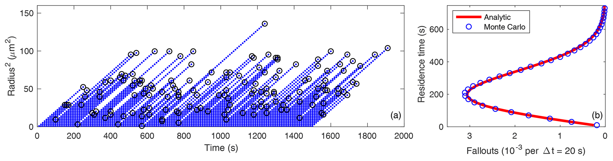
Figures 1 and 2 demonstrate that the r² and residence time distributions are closely related because each is determined by the droplet fallout process which is strongly affected by the stochastic vertical rearrangements of the droplets by the turbulent flow.

4 Analytic equilibrium solutions

We now derive the analytic equilibrium solutions for the distributions of r and r², v(r) and w(s), respectively.

4.1 Analytic equilibrium solution for the distribution of r

In a steady state, Eq. (2) becomes

$$\begin{array}{}\text{(8)}& \mathrm{0}=-{\displaystyle \frac{d}{\mathrm{d}r}}\left(\mathit{\xi }{\displaystyle \frac{v}{r}}\right)-v{\displaystyle \frac{k_{\mathrm{1}}}{h}}{r}^{\mathrm{2}}+A.\end{array}$$

If the production of (activated) droplets from the injected aerosol occurs only for $\mathrm{0}<r_{\mathrm{0}}<r<r_a$, and the loss due to sedimentation for r<r_a is negligible, then we can integrate Eq. (8) from r=r₀ to r=r_a to obtain

$$\mathrm{0}=-\underset{r_{\mathrm{0}}}{\overset{r_a}{\int }}{\displaystyle \frac{d}{\mathrm{d}r}}\left(\mathit{\xi }{\displaystyle \frac{v}{r}}\right)\mathrm{d}r+\underset{r_{\mathrm{0}}}{\overset{r_a}{\int }}A\mathrm{d}r,$$

which becomes

$$\mathrm{0}=-\left(\mathit{\xi }{\displaystyle \frac{v}{r}}\right){|}_{r_{\mathrm{0}}}^{r_a}+\underset{r_{\mathrm{0}}}{\overset{r_a}{\int }}A\mathrm{d}r,$$

then

$$\mathrm{0}=-\mathit{\xi }\left({\displaystyle \frac{v\left(r_a\right)}{r_a}}-{\displaystyle \frac{v\left(r_{\mathrm{0}}\right)}{r_{\mathrm{0}}}}\right)+\underset{r_{\mathrm{0}}}{\overset{r_a}{\int }}A\mathrm{d}r,$$

and finally, using v(r₀)=0,

$$\begin{array}{}\text{(9)}& {\displaystyle \frac{v\left(r_a\right)}{r_a}}={\displaystyle \frac{\mathrm{1}}{\mathit{\xi }}}\underset{r_{\mathrm{0}}}{\overset{r_a}{\int }}A\mathrm{d}r.\end{array}$$

Equation (9) allows us to consider the following ordinary differential equation (ODE) instead of Eq. (8) for $r_a<r<\mathrm{\infty }$:

$$\begin{array}{}\text{(10)}& \mathrm{0}=-{\displaystyle \frac{d}{\mathrm{d}r}}\left(\mathit{\xi }{\displaystyle \frac{v}{r}}\right)-v{\displaystyle \frac{k_{\mathrm{1}}}{h}}{r}^{\mathrm{2}},\end{array}$$

with the boundary condition at r=r_a given by Eq. (9). When the supersaturation is steady and uniform, ξ is a constant, so we can write Eq. (10) as

$$\begin{array}{}\text{(11)}& \mathrm{0}=-{\displaystyle \frac{d}{\mathrm{d}r}}\left({\displaystyle \frac{v}{r}}\right)-Cv{r}^{\mathrm{2}},\end{array}$$

where $C\equiv k_{\mathrm{1}}/\left(\mathit{\xi }h\right)$ is a constant with units of (length)⁻⁴. The general solution to Eq. (11) is

$$\begin{array}{}\text{(12)}& v\left(r\right)=Dr\exp (-C{r}^{\mathrm{4}}/\mathrm{4}),\end{array}$$

where D is an integration constant with units of (mass)⁻¹ (length)⁻² which can be determined from v(r_a)∕r_a, which in turn is given by Eq. (9):

$$\begin{array}{}\text{(13)}& D={\displaystyle \frac{v\left(r_a\right)}{r_a}}\exp (C{r}_a^{\mathrm{4}}/\mathrm{4}).\end{array}$$

Most of the solutions of the ordinary differential equations and integrals that appear in this study were obtained using Wolfram|Alpha (Wolfram Alpha LLC, 2019).

4.2 Analytic equilibrium solution for the distribution of r²

One way to derive w(s)=w(r²) is analogous to that for v(r). Another way is to recognize that $\mathit{\rho }v=\mathrm{d}N/\mathrm{d}r$ and $\mathit{\rho }w=\mathrm{d}N/\mathrm{d}s=\mathrm{d}N/\mathrm{d}{r}^{\mathrm{2}}$, where ρ is the air density and dN is the number of droplets per unit volume with r and r² in the intervals $[r,r+\mathrm{d}r]$ and $[r^{\mathrm{2}},r^{\mathrm{2}}+\mathrm{d}{r}^{\mathrm{2}}]$, respectively, from which we obtain d$N/\mathit{\rho }=v\mathrm{d}r=w\mathrm{d}{r}^{\mathrm{2}}$. Hence,

$$\begin{array}{}\text{(14)}& w={\displaystyle \frac{v}{\mathrm{d}{r}^{\mathrm{2}}/\mathrm{d}r}}={\displaystyle \frac{v}{\mathrm{2}r}}={\displaystyle \frac{D}{\mathrm{2}}}\exp (-C{r}^{\mathrm{4}}/\mathrm{4})=G\exp (-C{s}^{\mathrm{2}}/\mathrm{4}),\end{array}$$

using Eq. (12), s=r², and $G=D/\mathrm{2}$. Just as for the ODE (Eq. 10), the corresponding solution (Eq. 12) is valid only for $r>r_a>r_{\mathrm{0}}>\mathrm{0}$. Similarly, Eq. (14) is valid only for $s>s_a>s_{\mathrm{0}}>\mathrm{0}$.

4.3 Droplet number concentration and integration constant

As already noted, v(r) dr is the number of cloud droplets per unit mass of air with radii in the interval $[r,r+\mathrm{d}r]$. Therefore, the number of cloud droplets per unit volume of air is

$$\begin{array}{}\text{(15)}& \begin{array}{rl}N& =\mathit{\rho }\underset{\mathrm{0}}{\overset{\mathrm{\infty }}{\int }}v\left(r\right)\mathrm{d}r=\mathit{\rho }D\underset{\mathrm{0}}{\overset{\mathrm{\infty }}{\int }}r\exp (-C{r}^{\mathrm{4}}/\mathrm{4})\mathrm{d}r\\ & =\mathit{\rho }D{\displaystyle \frac{\sqrt{\mathit{\pi }}}{\mathrm{2}\sqrt{C}}},\end{array}\end{array}$$

where v(r) is given by Eq. (12). We see that N is related to both D and C. We can solve Eq. (15) for the integration constant D in Eq. (12):

$$\begin{array}{}\text{(16)}& D=N{\displaystyle \frac{\mathrm{2}\sqrt{C}}{\mathit{\rho }\sqrt{\mathit{\pi }}}}.\end{array}$$

The number of cloud droplets per unit volume with radii larger than a is

$$\begin{array}{}\text{(17)}& \begin{array}{rl}N\left(a\right)& =\mathit{\rho }\underset{a}{\overset{\mathrm{\infty }}{\int }}v\left(r\right)\mathrm{d}r=\mathit{\rho }D\underset{a}{\overset{\mathrm{\infty }}{\int }}r\exp (-C{r}^{\mathrm{4}}/\mathrm{4})\mathrm{d}r\\ & =\mathit{\rho }D{\displaystyle \frac{\sqrt{\mathit{\pi }}}{\mathrm{2}\sqrt{C}}}\mathrm{erfc}(a^{\mathrm{2}}\sqrt{C}/\mathrm{2})=N\mathrm{erfc}(a^{\mathrm{2}}\sqrt{C}/\mathrm{2}),\end{array}\end{array}$$

where $\mathrm{erfc}\left(z\right)\equiv \mathrm{1}-\mathrm{erf}\left(z\right)$ is the complementary error function. From Eq. (17), we obtain the fraction of the total number of droplets with radii larger than a,

$$\begin{array}{}\text{(18)}& f\left(a\right)\equiv {\displaystyle \frac{N\left(a\right)}{N}}=\mathrm{erfc}\left({\displaystyle \frac{a^{\mathrm{2}}\sqrt{C}}{\mathrm{2}}}\right).\end{array}$$

4.4 PDFs of the equilibrium droplet size distribution

The PDF of the droplet radius distribution given by Eq. (12) is

$$\begin{array}{}\text{(19)}& p\left(r\right)={\displaystyle \frac{\mathit{\rho }v\left(r\right)}{N}}={\displaystyle \frac{\mathrm{2}\sqrt{C}}{\sqrt{\mathit{\pi }}}}r\exp (-C{r}^{\mathrm{4}}/\mathrm{4}).\end{array}$$

The PDF of the droplet squared radius distribution given by Eq. (14) is

$$\begin{array}{}\text{(20)}& q\left(s\right)={\displaystyle \frac{\mathit{\rho }w\left(s\right)}{N}}={\displaystyle \frac{\sqrt{C}}{\sqrt{\mathit{\pi }}}}\exp (-C{s}^{\mathrm{2}}/\mathrm{4}).\end{array}$$

Both depend only on C. Figures 3 and 4 display p(r) and q(s), respectively, for a supersaturation of 0.1 % and h=1 m.

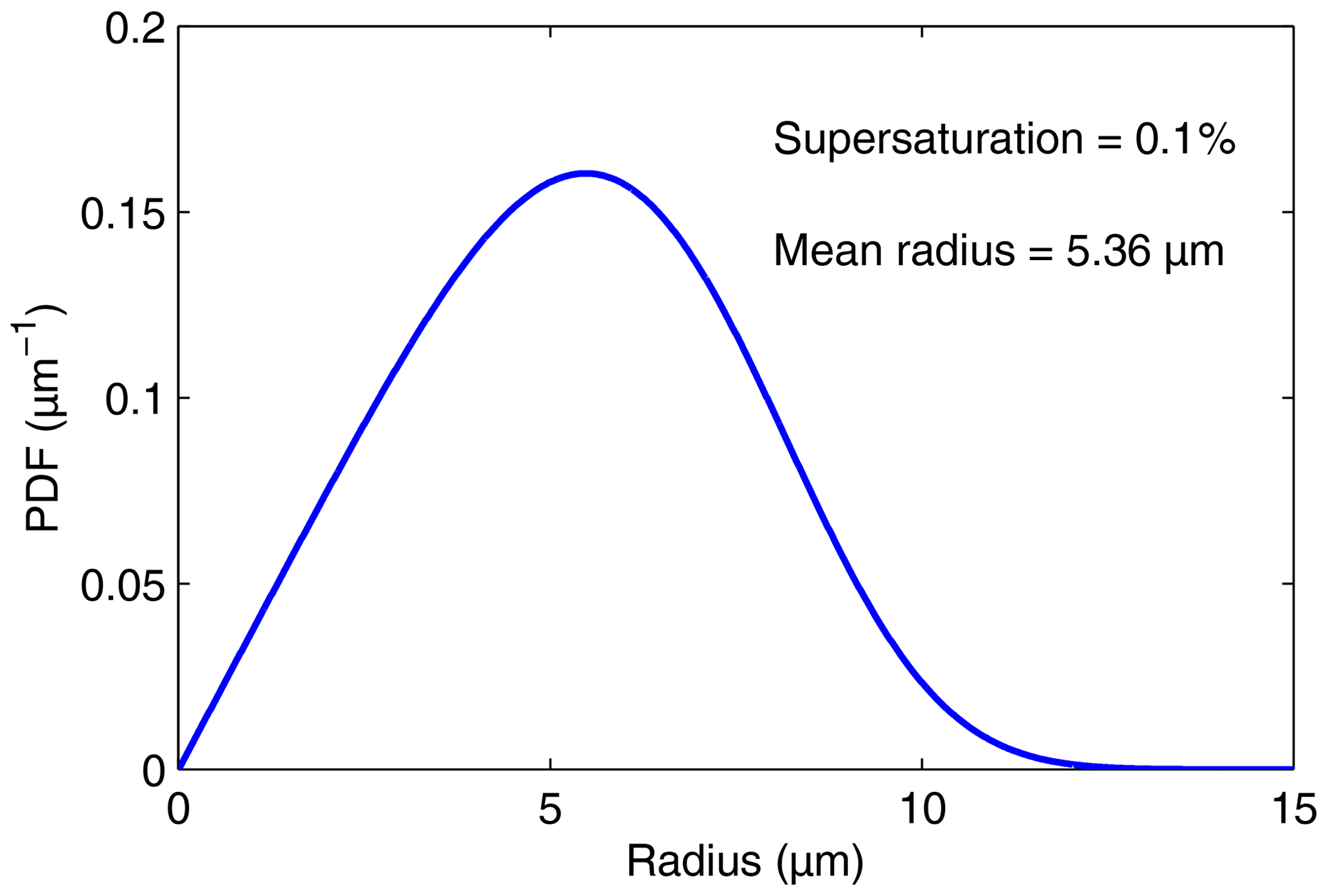
Figure 3 PDF of the droplet radius distribution given by Eq. (19) for a supersaturation of 0.1 % and h=1 m.

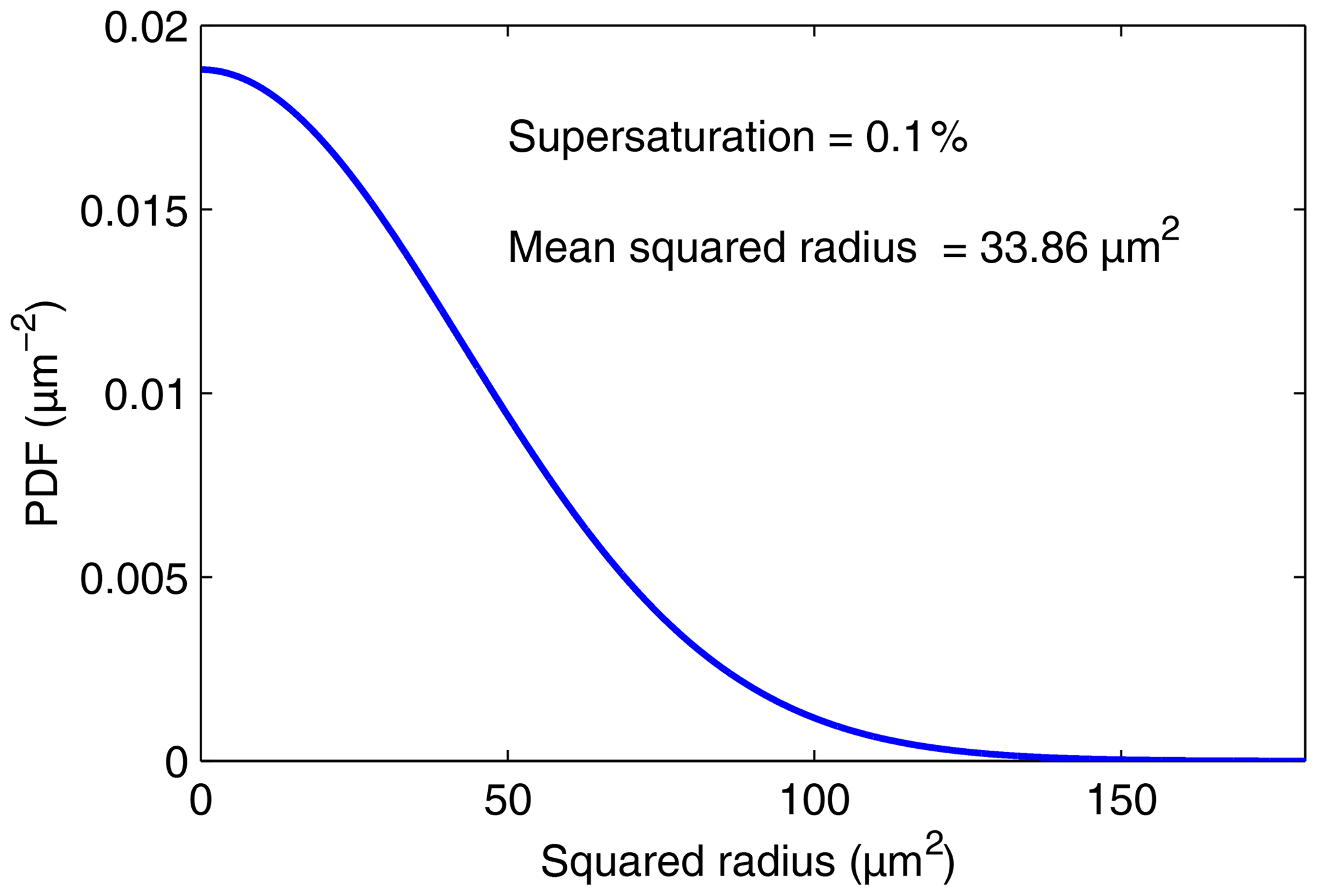
Figure 4 PDF of the droplet squared radius distribution given by Eq. (20) for a supersaturation of 0.1 % and h=1 m.

By changing the independent variable from s≡r² to the non-dimensional variable $y\equiv s\sqrt{C}/\mathrm{2}$, we obtain the non-dimensional PDF,

$$\begin{array}{}\text{(21)}& Q\left(y\right)={\displaystyle \frac{\mathrm{2}}{\sqrt{\mathit{\pi }}}}\exp (-y^{\mathrm{2}}).\end{array}$$

4.5 Median radius and CDF of the equilibrium droplet size distribution

The median radius, $\stackrel{\mathrm{̃}}{r}$, is defined by

$$\underset{\mathrm{0}}{\overset{\stackrel{\mathrm{̃}}{r}}{\int }}p\left(r\right)\mathrm{d}r=\mathrm{0.5}.$$

The cumulative density function (CDF) is the integral from 0 to R of p(r):

$$\begin{array}{}\text{(22)}& I\left(R\right)\equiv \underset{\mathrm{0}}{\overset{R}{\int }}p\left(r\right)\mathrm{d}r=\mathrm{1}-f\left(R\right)=\mathrm{erf}\left({\displaystyle \frac{\sqrt{C}{R}^{\mathrm{2}}}{\mathrm{2}}}\right),\end{array}$$

where f(R) is given by Eq. (18). One can use Eq. (22) to determine C given R for any percentile I of the cumulative distribution function. In general,

$$\begin{array}{}\text{(23)}& \sqrt{C}={\displaystyle \frac{\mathrm{2}}{R^{\mathrm{2}}}}{\mathrm{erf}}^{-\mathrm{1}}\left(I\right).\end{array}$$

If given the median radius, $\stackrel{\mathrm{̃}}{r}$, then I=0.5 and

$$\sqrt{C}={\displaystyle \frac{\mathrm{2}}{{\stackrel{\mathrm{̃}}{r}}^{\mathrm{2}}}}{\mathrm{erf}}^{-\mathrm{1}}\left(\mathrm{0.5}\right)\approx {\displaystyle \frac{\mathrm{0.953873}}{{\stackrel{\mathrm{̃}}{r}}^{\mathrm{2}}}},$$

so that

$$\begin{array}{}\text{(24)}& C\approx {\displaystyle \frac{\mathrm{0.909873}}{{\stackrel{\mathrm{̃}}{r}}^{\mathrm{4}}}}.\end{array}$$

4.6 Mode radius

We derive the mode radius, $\widehat{r}$, by expanding the derivative in Eq. (11) to obtain

$$\mathrm{0}={\displaystyle \frac{\mathrm{d}v}{\mathrm{d}r}}-{\displaystyle \frac{v}{r}}+Cv{r}^{\mathrm{3}},$$

then applying $(\mathrm{d}v/\mathrm{d}r{)}_{r=\widehat{r}}=\mathrm{0}$ and solving for ${\widehat{r}}^{\mathrm{4}}$:

$$\begin{array}{}\text{(25)}& {\widehat{r}}^{\mathrm{4}}={\displaystyle \frac{\mathrm{1}}{C}}={\displaystyle \frac{\mathit{\xi }h}{k_{\mathrm{1}}}}.\end{array}$$

The relationship between the supersaturation and the mode radius for h=1 m is shown in Fig. 5. This plot indicates that as the supersaturation increases by 4 orders of magnitude, from 0.001 % to 10 %, the mode radius increases from about 2 to 17 µm.

Figure 5 The mode radius versus the supersaturation for h=1 m as given by Eq. (25).

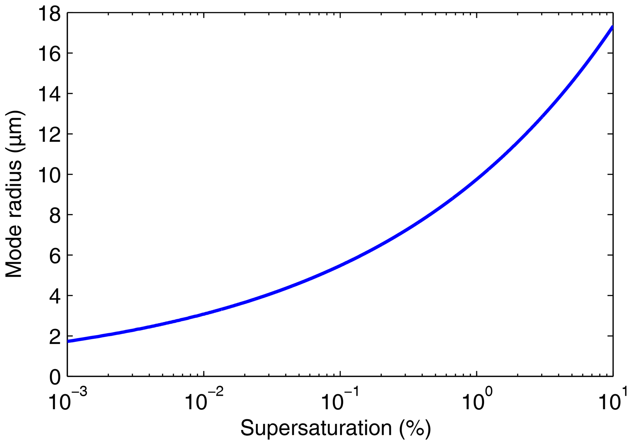
By writing Eq. (25) in the form

$${\displaystyle \frac{{\widehat{r}}^{\mathrm{2}}}{\mathit{\xi }}}={\displaystyle \frac{h}{k_{\mathrm{1}}{\widehat{r}}^{\mathrm{2}}}},$$

we see from Eq. (6) that $\widehat{r}$ is the droplet radius for which the timescale for droplet number growth due to condensation, r²∕ξ, equals the timescale for droplet number depletion due to sedimentation, $h/u=h/\left(k_{\mathrm{1}}{r}^{\mathrm{2}}\right)$.

5 Moments derived from the analytic equilibrium PDFs

5.1 Mean radius

The mean radius is

$$\begin{array}{}\text{(26)}& \begin{array}{rl}\stackrel{\mathrm{‾}}{r}& =\underset{\mathrm{0}}{\overset{\mathrm{\infty }}{\int }}rp\left(r\right)\mathrm{d}r={\displaystyle \frac{\mathrm{2}\sqrt{C}}{\sqrt{\mathit{\pi }}}}\underset{\mathrm{0}}{\overset{\mathrm{\infty }}{\int }}{r}^{\mathrm{2}}\exp (-C{r}^{\mathrm{4}}/\mathrm{4})\mathrm{d}r\\ & ={\displaystyle \frac{\sqrt{\mathrm{2}}}{\sqrt{\mathit{\pi }}}}{\displaystyle \frac{\mathrm{\Gamma }\left(\frac{\mathrm{3}}{\mathrm{4}}\right)}{C^{\mathrm{1}/\mathrm{4}}}},\end{array}\end{array}$$

which depends only on C. Solve this for C^1∕4 to obtain

$$C^{\mathrm{1}/\mathrm{4}}={\displaystyle \frac{\sqrt{\mathrm{2}}}{\sqrt{\mathit{\pi }}}}{\displaystyle \frac{\mathrm{\Gamma }\left(\frac{\mathrm{3}}{\mathrm{4}}\right)}{\stackrel{\mathrm{‾}}{r}}},$$

so

$$\begin{array}{}\text{(27)}& C\approx {\displaystyle \frac{\mathrm{0.913893}}{{\stackrel{\mathrm{‾}}{r}}^{\mathrm{4}}}}.\end{array}$$

Equations (24) and (27) imply that

$${\displaystyle \frac{\stackrel{\mathrm{̃}}{r}}{\stackrel{\mathrm{‾}}{r}}}\approx \mathrm{0.998898}.$$

The mean radius of droplets with radii larger than a is

$$\begin{array}{}\text{(28)}& \begin{array}{rl}\stackrel{\mathrm{‾}}{r}\left(a\right)& ={\displaystyle \frac{{\int }_a^{\mathrm{\infty }}rp\left(r\right)\mathrm{d}r}{{\int }_a^{\mathrm{\infty }}p\left(r\right)\mathrm{d}r}}={\displaystyle \frac{\frac{\mathrm{2}\sqrt{C}}{\sqrt{\mathit{\pi }}}{\int }_a^{\mathrm{\infty }}{r}^{\mathrm{2}}\exp (-C{r}^{\mathrm{4}}/\mathrm{4})\mathrm{d}r}{f\left(a\right)}}\\ & ={\displaystyle \frac{\frac{\sqrt{\mathrm{2}}}{\sqrt{\mathit{\pi }}}\frac{\mathrm{\Gamma }(\frac{\mathrm{3}}{\mathrm{4}},\frac{a^{\mathrm{4}}C}{\mathrm{4}})}{C^{\mathrm{1}/\mathrm{4}}}}{\mathrm{erfc}\left(\frac{a^{\mathrm{2}}\sqrt{C}}{\mathrm{2}}\right)}},\end{array}\end{array}$$

where f(a) is the fraction of the total number of droplets with radii larger than a and Γ(b,x) is the upper incomplete gamma function. Because

$$\underset{a}{\overset{\mathrm{\infty }}{\int }}p\left(r\right)\mathrm{d}r={\displaystyle \frac{N\left(a\right)}{N}},$$

we can use

$${\displaystyle \frac{N\left(a\right)}{N}}\equiv f\left(a\right)=\mathrm{erfc}\left({\displaystyle \frac{a^{\mathrm{2}}\sqrt{C}}{\mathrm{2}}}\right),$$

from Eq. (18). The upper incomplete gamma function is defined here as

$$\mathrm{\Gamma }(b,x)\equiv \underset{x}{\overset{\mathrm{\infty }}{\int }}{t}^{b-\mathrm{1}}{e}^{-t}\mathrm{d}t.$$

Note that the MATLAB^® upper incomplete gamma function is defined differently, as

$${\displaystyle \frac{\mathrm{1}}{\mathrm{\Gamma }\left(b\right)}}\underset{x}{\overset{\mathrm{\infty }}{\int }}{t}^{b-\mathrm{1}}{e}^{-t}\mathrm{d}t,$$

and is called using gammainc(x,b,'upper'); note the reversed argument order.

5.2 Mean squared radius

The mean of the squared radius is

$$\begin{array}{}\text{(29)}& \stackrel{\mathrm{‾}}{r^{\mathrm{2}}}=\underset{\mathrm{0}}{\overset{\mathrm{\infty }}{\int }}sq\left(s\right)\mathrm{d}s={\displaystyle \frac{\sqrt{C}}{\sqrt{\mathit{\pi }}}}\underset{\mathrm{0}}{\overset{\mathrm{\infty }}{\int }}s\exp (-C{s}^{\mathrm{2}}/\mathrm{4})\mathrm{d}s={\displaystyle \frac{\mathrm{2}}{\sqrt{\mathit{\pi }}\sqrt{C}}},\end{array}$$

which depends only on C. Solve for C:

$$\begin{array}{}\text{(30)}& C={\displaystyle \frac{\mathrm{4}}{\mathit{\pi }(\stackrel{\mathrm{‾}}{r^{\mathrm{2}}}{)}^{\mathrm{2}}}}\approx {\displaystyle \frac{\mathrm{1.273240}}{(\stackrel{\mathrm{‾}}{r^{\mathrm{2}}}{)}^{\mathrm{2}}}}.\end{array}$$

Equations (27) and (30) imply that

$$\begin{array}{}\text{(31)}& {\displaystyle \frac{\stackrel{\mathrm{‾}}{r^{\mathrm{2}}}}{{\stackrel{\mathrm{‾}}{r}}^{\mathrm{2}}}}\approx \mathrm{1.180341}.\end{array}$$

The mean of the squared radius of droplets with radii larger than a is

$$\begin{array}{}\text{(32)}& \begin{array}{rl}\stackrel{\mathrm{‾}}{r^{\mathrm{2}}}\left(a\right)& ={\displaystyle \frac{{\int }_{a^{\mathrm{2}}}^{\mathrm{\infty }}sq\left(s\right)\mathrm{d}s}{{\int }_{a^{\mathrm{2}}}^{\mathrm{\infty }}q\left(s\right)\mathrm{d}s}}={\displaystyle \frac{\frac{\sqrt{C}}{\sqrt{\mathit{\pi }}}{\int }_{a^{\mathrm{2}}}^{\mathrm{\infty }}s\exp (-C{s}^{\mathrm{2}}/\mathrm{4})\mathrm{d}s}{f\left(a\right)}}\\ & ={\displaystyle \frac{\frac{\mathrm{2}}{\sqrt{\mathit{\pi }}\sqrt{C}}\exp (-a^{\mathrm{4}}C/\mathrm{4})}{\mathrm{erfc}\left(\frac{a^{\mathrm{2}}\sqrt{C}}{\mathrm{2}}\right)}}.\end{array}\end{array}$$

5.3 Mean cubed radius

The mean cubed radius is

$$\begin{array}{}\text{(33)}& \begin{array}{rl}\stackrel{\mathrm{‾}}{r^{\mathrm{3}}}& =\underset{\mathrm{0}}{\overset{\mathrm{\infty }}{\int }}{r}^{\mathrm{3}}p\left(r\right)\mathrm{d}r={\displaystyle \frac{\mathrm{2}\sqrt{C}}{\sqrt{\mathit{\pi }}}}\underset{\mathrm{0}}{\overset{\mathrm{\infty }}{\int }}{r}^{\mathrm{4}}\exp (-C{r}^{\mathrm{4}}/\mathrm{4})\mathrm{d}r\\ & ={\displaystyle \frac{\mathrm{2}\sqrt{\mathrm{2}}}{\sqrt{\mathit{\pi }}}}{\displaystyle \frac{\mathrm{\Gamma }\left(\frac{\mathrm{5}}{\mathrm{4}}\right)}{C^{\mathrm{3}/\mathrm{4}}}},\end{array}\end{array}$$

which depends only on C. Solve Eq. (33) for C:

$$\begin{array}{}\text{(34)}& C={\displaystyle \frac{\mathrm{4}}{{\mathit{\pi }}^{\mathrm{2}/\mathrm{3}}}}{\left({\displaystyle \frac{\mathrm{\Gamma }\left(\frac{\mathrm{5}}{\mathrm{4}}\right)}{\stackrel{\mathrm{‾}}{r^{\mathrm{3}}}}}\right)}^{\mathrm{4}/\mathrm{3}}\approx {\displaystyle \frac{\mathrm{1.635767}}{(\stackrel{\mathrm{‾}}{r^{\mathrm{3}}}{)}^{\mathrm{4}/\mathrm{3}}}}.\end{array}$$

Equations (26) and (33) imply that

$$\begin{array}{}\text{(35)}& {\displaystyle \frac{\stackrel{\mathrm{‾}}{r^{\mathrm{3}}}}{{\stackrel{\mathrm{‾}}{r}}^{\mathrm{3}}}}={\displaystyle \frac{\mathit{\pi }\mathrm{\Gamma }\left(\frac{\mathrm{5}}{\mathrm{4}}\right)}{\mathrm{\Gamma }{\left(\frac{\mathrm{3}}{\mathrm{4}}\right)}^{\mathrm{3}}}}\approx \mathrm{1.547460}.\end{array}$$

The mean cubed radius of droplets with radii larger than a is

$$\begin{array}{}\text{(36)}& \begin{array}{rl}\stackrel{\mathrm{‾}}{r^{\mathrm{3}}}\left(a\right)& ={\displaystyle \frac{{\int }_a^{\mathrm{\infty }}{r}^{\mathrm{3}}p\left(r\right)\mathrm{d}r}{{\int }_a^{\mathrm{\infty }}p\left(r\right)\mathrm{d}r}}={\displaystyle \frac{\frac{\mathrm{2}\sqrt{C}}{\sqrt{\mathit{\pi }}}{\int }_a^{\mathrm{\infty }}{r}^{\mathrm{4}}\exp (-C{r}^{\mathrm{4}}/\mathrm{4})\mathrm{d}r}{f\left(a\right)}}\\ & ={\displaystyle \frac{\frac{\mathrm{2}\sqrt{\mathrm{2}}}{\sqrt{\mathit{\pi }}}\frac{\mathrm{\Gamma }\left(\frac{\mathrm{5}}{\mathrm{4}},\frac{a^{\mathrm{4}}C}{\mathrm{4}}\right)}{C^{\mathrm{3}/\mathrm{4}}}}{\mathrm{erfc}\left(\frac{a^{\mathrm{2}}\sqrt{C}}{\mathrm{2}}\right)}}.\end{array}\end{array}$$

5.4 Mean r⁴

The mean r⁴ is

$$\begin{array}{}\text{(37)}& \stackrel{\mathrm{‾}}{r^{\mathrm{4}}}=\underset{\mathrm{0}}{\overset{\mathrm{\infty }}{\int }}{r}^{\mathrm{4}}p\left(r\right)\mathrm{d}r={\displaystyle \frac{\mathrm{2}\sqrt{C}}{\sqrt{\mathit{\pi }}}}\underset{\mathrm{0}}{\overset{\mathrm{\infty }}{\int }}{r}^{\mathrm{5}}\exp (-C{r}^{\mathrm{4}}/\mathrm{4})\mathrm{d}r={\displaystyle \frac{\mathrm{2}}{C}},\end{array}$$

which depends only on C. Solve Eq. (37) for C:

$$\begin{array}{}\text{(38)}& C={\displaystyle \frac{\mathrm{2}}{\stackrel{\mathrm{‾}}{r^{\mathrm{4}}}}}.\end{array}$$

Equations (26) and (37) imply that

$$\begin{array}{}\text{(39)}& {\displaystyle \frac{\stackrel{\mathrm{‾}}{r^{\mathrm{4}}}}{{\stackrel{\mathrm{‾}}{r}}^{\mathrm{4}}}}={\displaystyle \frac{{\mathit{\pi }}^{\mathrm{2}}}{\mathrm{2}\mathrm{\Gamma }(\frac{\mathrm{3}}{\mathrm{4}}{)}^{\mathrm{4}}}}\approx \mathrm{2.188440}.\end{array}$$

The mean r⁴ of droplets with radii larger than a is

$$\begin{array}{}\text{(40)}& \begin{array}{rl}\stackrel{\mathrm{‾}}{r^{\mathrm{4}}}\left(a\right)& ={\displaystyle \frac{{\int }_a^{\mathrm{\infty }}{r}^{\mathrm{4}}p\left(r\right)\mathrm{d}r}{{\int }_a^{\mathrm{\infty }}p\left(r\right)\mathrm{d}r}}={\displaystyle \frac{\frac{\mathrm{2}\sqrt{C}}{\sqrt{\mathit{\pi }}}{\int }_a^{\mathrm{\infty }}{r}^{\mathrm{5}}\exp (-C{r}^{\mathrm{4}}/\mathrm{4})\mathrm{d}r}{f\left(a\right)}}\\ & ={\displaystyle \frac{\mathrm{2}}{C}}+{\displaystyle \frac{\frac{\mathrm{2}{a}^{\mathrm{2}}}{\sqrt{\mathit{\pi }}\sqrt{C}}\exp (-a^{\mathrm{4}}C/\mathrm{4})}{\mathrm{erfc}\left(\frac{a^{\mathrm{2}}\sqrt{C}}{\mathrm{2}}\right)}}.\end{array}\end{array}$$

5.5 Mean r⁵

The mean r⁵ is

$$\begin{array}{}\text{(41)}& \begin{array}{rl}\stackrel{\mathrm{‾}}{r^{\mathrm{5}}}& =\underset{\mathrm{0}}{\overset{\mathrm{\infty }}{\int }}{r}^{\mathrm{5}}p\left(r\right)\mathrm{d}r={\displaystyle \frac{\mathrm{2}\sqrt{C}}{\sqrt{\mathit{\pi }}}}\underset{\mathrm{0}}{\overset{\mathrm{\infty }}{\int }}{r}^{\mathrm{6}}\exp (-C{r}^{\mathrm{4}}/\mathrm{4})\mathrm{d}r\\ & ={\displaystyle \frac{\mathrm{4}\sqrt{\mathrm{2}}}{\sqrt{\mathit{\pi }}}}{\displaystyle \frac{\mathrm{\Gamma }(\mathrm{7}/\mathrm{4})}{C^{\mathrm{5}/\mathrm{4}}}},\end{array}\end{array}$$

which depends only on C. Solve Eq. (41) for C:

$$\begin{array}{}\text{(42)}& C={\displaystyle \frac{\mathrm{4}}{{\mathit{\pi }}^{\mathrm{2}/\mathrm{5}}}}{\left({\displaystyle \frac{\mathrm{\Gamma }\left(\frac{\mathrm{7}}{\mathrm{4}}\right)}{\stackrel{\mathrm{‾}}{r^{\mathrm{5}}}}}\right)}^{\mathrm{4}/\mathrm{5}}\approx {\displaystyle \frac{\mathrm{2.365245}}{(\stackrel{\mathrm{‾}}{r^{\mathrm{5}}}{)}^{\mathrm{4}/\mathrm{5}}}}.\end{array}$$

The mean r⁵ of droplets with radii larger than a is

$$\begin{array}{}\text{(43)}& \begin{array}{rl}\stackrel{\mathrm{‾}}{r^{\mathrm{5}}}\left(a\right)& ={\displaystyle \frac{{\int }_a^{\mathrm{\infty }}{r}^{\mathrm{5}}p\left(r\right)\mathrm{d}r}{{\int }_a^{\mathrm{\infty }}p\left(r\right)\mathrm{d}r}}={\displaystyle \frac{\frac{\mathrm{2}\sqrt{C}}{\sqrt{\mathit{\pi }}}{\int }_a^{\mathrm{\infty }}{r}^{\mathrm{6}}\exp (-C{r}^{\mathrm{4}}/\mathrm{4})\mathrm{d}r}{f\left(a\right)}}\\ & ={\displaystyle \frac{\frac{\frac{\mathrm{4}\sqrt{\mathrm{2}}}{\sqrt{\mathit{\pi }}}\mathrm{\Gamma }(\mathrm{7}/\mathrm{4},\frac{a^{\mathrm{4}}C}{\mathrm{4}})}{C^{\mathrm{5}/\mathrm{4}}}}{\mathrm{erfc}\left(\frac{a^{\mathrm{2}}\sqrt{C}}{\mathrm{2}}\right)}}.\end{array}\end{array}$$

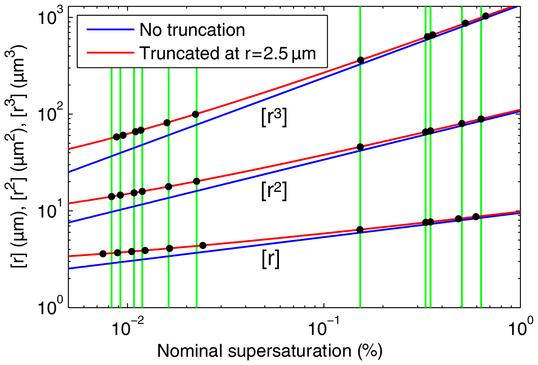
Figure 6 Mean radius, [r], mean squared radius, [r²], and cubed mean radius, [r³], versus nominal mean supersaturation for h=1 m for DSDs with no truncation (blue) and for DSDs truncated at r=2.5 µm (red). The black dots indicate the nominal mean supersaturation values implied by [r], [r²], and [r³] obtained from 11 measured DSDs truncated at r=2.5 µm (Chandrakar et al., 2018b). The vertical green lines pass through the nominal mean supersaturation values implied by the measured [r²] values and allow a visual assessment of the consistency of the supersaturation values implied by the three measured moments for each of the 11 DSDs.

6 Consistency between analytical and measured DSDs

This study was motivated by the question of whether fluctuations in supersaturation are needed to explain the steady-state DSDs measured in the Michigan Tech turbulent cloud chamber (Π chamber) under conditions of constant aerosol injection rate. In this section, we use statistics from a set of measured DSDs to check for consistency with the analytic DSD, which was derived neglecting droplet curvature and solute effects, the effects of supersaturation fluctuations, and deviations from Stokes' fall speed.

We use statistics from a set of 11 DSDs with a wide range of droplet number concentrations (Chandrakar et al., 2018b) which were measured by Chandrakar et al. (2018c) when the temperature difference between the top and bottom boundaries was 19 K. The DSDs were measured using a phase Doppler interferometer and were truncated at a radius of 2.5 µm because smaller droplets were not reliably detected (Chandrakar et al., 2018a). Measurements were made over an interval of about 200 min for each DSD.

Do we expect the neglect of droplet curvature and solute effects in the analytic DSDs to significantly affect the comparison of analytic and measured DSDs? The distributions of the dry diameters of the injected NaCl aerosol particles for the measured DSDs are approximately lognormal, with a mode diameter of 40 to 60 nm and a standard deviation of about 30 nm (Chandrakar et al., 2018b). For a mode diameter of 60 nm – which corresponds to a mean diameter of about 80 nm in a lognormal distribution – and a standard deviation of 30 nm, 99 % of the injected aerosol particles have diameters less than about 170 nm. For NaCl aerosol particles with a dry diameter of 170 nm, the critical radius $r^{*}\approx \mathrm{1.5}$ µm (Rogers and Yau, 1989). Because the truncation radius of 2.5 µm is larger than r^*, solute effects should generally be negligible. However, droplet curvature affects the equilibrium saturation ratio for droplets with radii larger than r^*, as shown by Fig. 6.2 in Rogers and Yau (1989). The potential impacts of both droplet curvature and solute effects on comparisons of analytic and measured DSDs will be discussed below, in Sect. 6.2.

6.1 Supersaturation inferred from measured moments

Because the PDF of the equilibrium droplet radius distribution, Eq. (19), depends only on $C\equiv k_{\mathrm{1}}/\left(\mathit{\xi }h\right)$, the moments of the PDF also depend only on C. The dependence of the first five moments on C are given by Eqs. (26), (29), (33), (37), and (41). Measurements of one or more moments would allow one to determine C.

However, measured DSDs are often truncated due to a lack of detectability of small cloud droplets or difficulty in differentiating unactivated aerosol particles from small cloud droplets. To deal with such DSDs, we derived the dependence of the first five moments of the droplet radius on C and the truncation radius, a. These are given by Eqs. (28), (32), (36), (40), and (43). With these, one can determine C from a moment and the DSD's truncation radius.

Knowing C, one can solve for the supersaturation, S−1, given k₁, h, and the thermodynamic parameter $(F_k+F_{\mathrm{d}}){}^{-\mathrm{1}}$. If the droplets fall at their Stokes' fall speeds, then k₁ is Stokes' fall speed parameter, which is known. However, if the droplet fall speeds are affected by turbophoresis or thermophoresis, for example, then the fall speed parameter may not be known. Even if the actual fall speed parameter is unknown, it is still useful to calculate the supersaturation from C using k₁ equal to Stokes' fall speed parameter. We call this the “nominal supersaturation.”

In Fig. 6 we plotted the mean radius, [r], mean squared radius , [r²], and mean cubed radius, [r³], versus the nominal mean supersaturation for h=1 m for DSDs with no truncation (blue) and for DSDs truncated at r=2.5 µm (red). The black dots indicate the nominal mean supersaturation values implied by [r], [r²], and [r³] obtained from 11 measured DSDs truncated at r=2.5 µm (Chandrakar et al., 2018b). The inferred nominal mean supersaturations range from 0.008 % to 0.6 %. The vertical green lines pass through the nominal mean supersaturation values implied by the measured [r²] values and allow a visual assessment of the consistency of the supersaturation values implied by the three measured moments for each of the 11 DSDs.

If each DSD measured in the Π chamber were determined by the mean supersaturation alone, we would expect all three of the moments from a DSD to imply the same nominal mean supersaturation. However, even if moments of the analytic PDF derived in this study are consistent with the corresponding measured moments, that would not prove that supersaturation fluctuations were absent. It could be that the effects of supersaturation fluctuations on the PDF are nearly the same as those of the mean supersaturation and are therefore difficult to discern. Or it could be that the effects are small despite the fluctuations being significant due to a low correlation between the fluctuations of supersaturation and droplet radius (Chandrakar et al., 2016).

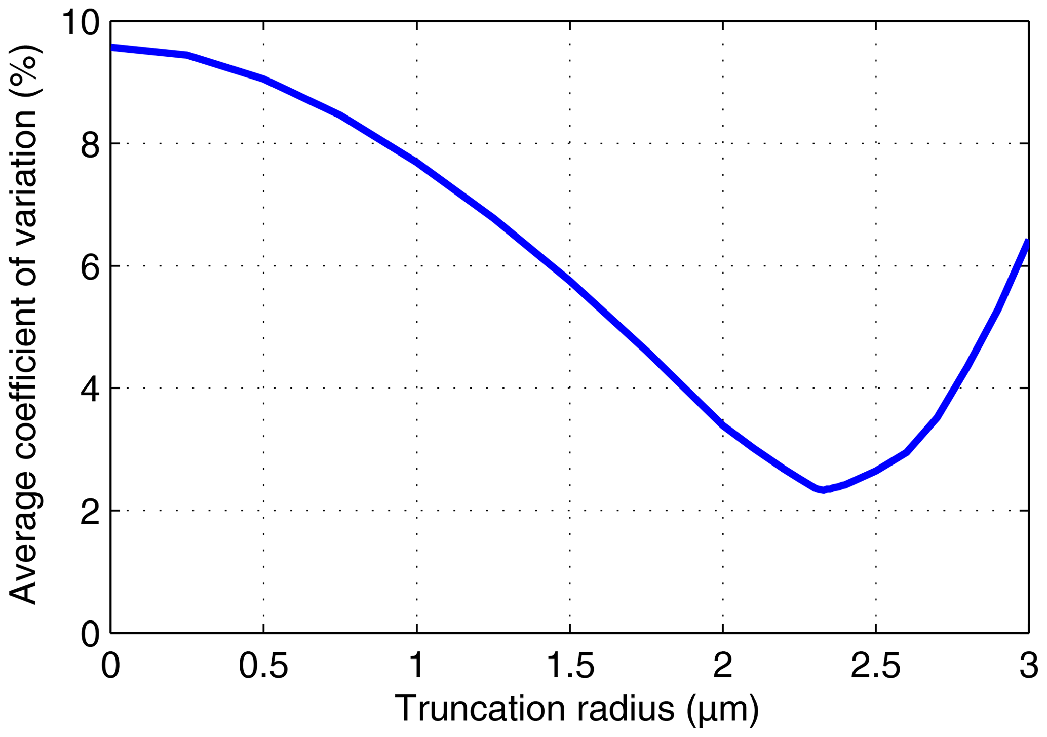
Figure 7 Average over the 11 DSDs of the coefficient of variation of the nominal mean supersaturation values implied by the three measured moments versus the truncation radius.

Figure 7 quantifies the degree of consistency of the three measured moments with the corresponding derived moments for truncation radii ranging from 0 to 3 µm. For each of the 11 DSDs, we used the supersaturation values implied by each of the three moments to calculate the mean and standard deviation of the implied supersaturation. We then calculated the average coefficient of variation of the implied supersaturation, which is plotted versus truncation radius in Fig. 7. The average coefficient of variation exhibits a pronounced minimum at r≈2.3 µm, which is nearly the same radius as the reported truncation radius (r=2.5 µm). Such agreement is expected if (1) the derived PDF is similar to the measured PDF and (2) the actual truncation radius is about 2.5 µm. The value of the average coefficient of variation at the truncation radius is a measure of the degree of consistency of the three measured moments with the corresponding derived moments. The value obtained (∼2.5 %) could be compared to values obtained using other PDFs, such as ones that include the effects of supersaturation fluctuations.

In Fig. 7, the minimum value of the average coefficient of variation is less than 25 % of the no-truncation value, which demonstrates that it is essential to consider the truncation radius when comparing theoretical moments to moments from a measured but truncated DSD. Figure 9 in Sect. 7.2 adds further support to this conclusion.

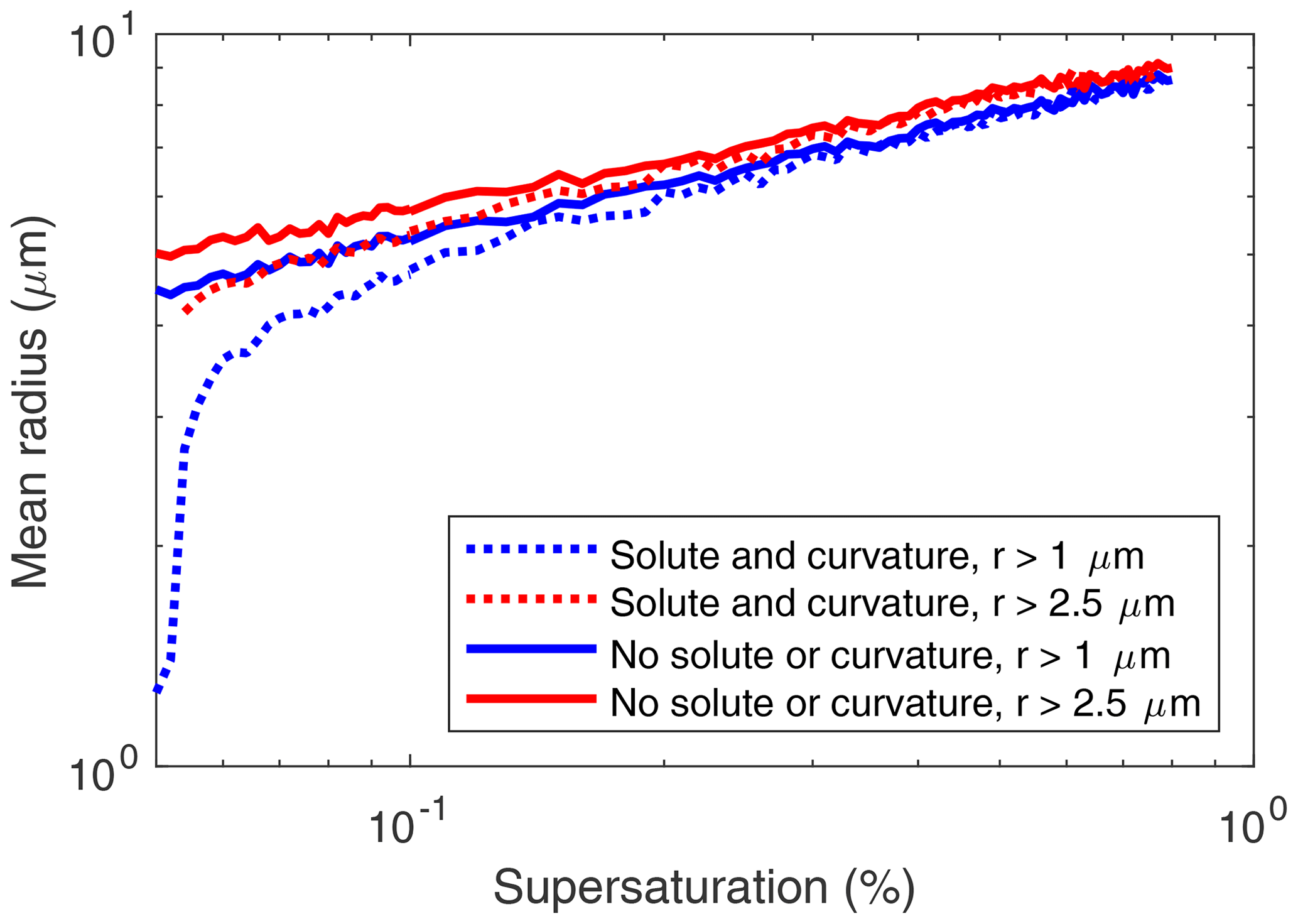
Figure 8 Mean droplet radius versus supersaturation from the Monte Carlo model: with solute and droplet curvature effects (dotted lines) and without (solid lines) for all droplets (blue) and excluding droplets with radii < 2.5 µm.

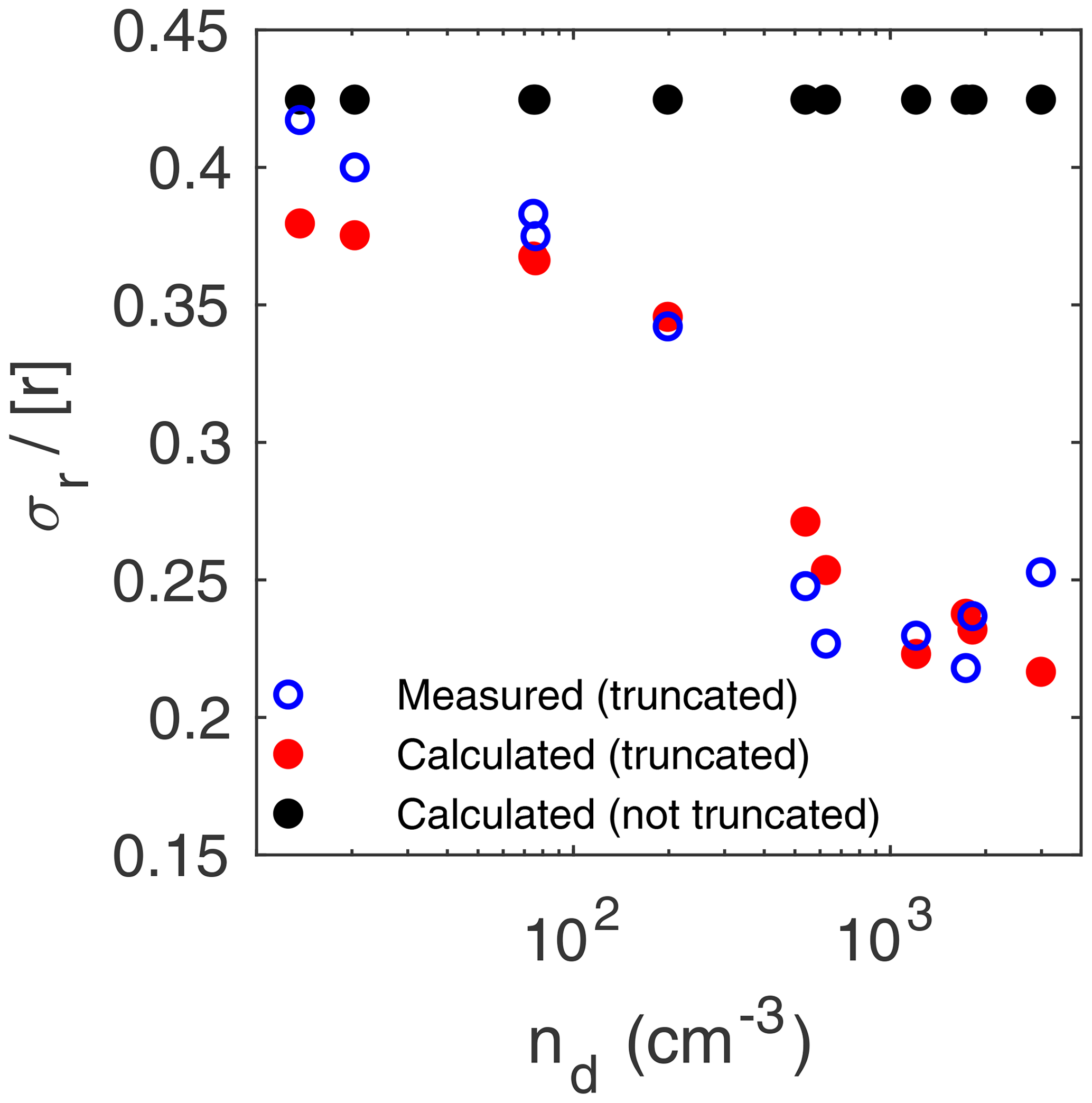
Figure 9 Relative dispersion of the radius versus droplet number concentration. The measured values of dispersion are from DSDs truncated at r=2.5 µm (blue circles) (Chandrakar et al., 2018b). The calculated values of dispersion used the average C implied by the three measured moments for each of the 11 DSDs. They were obtained by assuming either DSDs truncated at r=2.5 µm (red dots) or not truncated (black dots) and used Eqs. (46) and (28) or (47), respectively, with h=1 m.

6.2 Inferred mean supersaturation and droplet activation

Figure 6 shows that the inferred nominal mean supersaturations range from 0.008 % to 0.6 %. It is of interest to compare the range of the inferred mean supersaturations to the range of critical supersaturations for the measured injected aerosol size distributions. We noted above that for a mode diameter of 60 nm and a standard deviation of 30 nm, 99 % of the aerosol particles have a diameter less than about 170 nm. The critical supersaturation for a NaCl particle with a dry diameter of 170 nm is 0.052 %. In other words, about 1 % of the injected aerosols would be activated with a mean supersaturation of 0.052 %. What does this imply for the six DSDs in Fig. 6 with inferred mean supersaturations that are considerably less than 0.052 %? There are several possibilities, and they are not mutually exclusive.

1. Neglecting droplet curvature and solute effects in the analytic DSD governing equation produces significant underestimates of the inferred supersaturations. It could be that once curvature and solute effects are included in the droplet growth equation, the inferred mean supersaturations for all 11 measured DSDs will be large enough to activate at least the largest of the injected aerosols. To investigate this possibility, we used the droplet growth equation, both with and without the curvature and solute terms included, in the Monte Carlo model described in Sect. 3 to calculate mean droplet radius versus supersaturation for 100 supersaturation values (Fig. 8). With the curvature and solute terms included, the equation for the droplet growth rate becomes

   $$r{\displaystyle \frac{\mathrm{d}r}{\mathrm{d}t}}={\displaystyle \frac{(S-\mathrm{1})-\frac{a}{r}+\frac{b}{r^{\mathrm{3}}}}{F_k+F_{\mathrm{d}}}},$$

   where $-a/r$ is the curvature term, and b∕r³ is the solute term (Rogers and Yau, 1989). Figure 8 shows that the mean droplet radius is smaller when these terms are included, for the same fixed supersaturation. This is due to the slower initial growth of the droplets. The differences in mean radius are largest for supersaturations slightly larger than the critical supersaturation.

   How do the curvature and solute terms affect the inferred supersaturation? For a given droplet radius, the inferred supersaturation is larger with solute and curvature terms included. In our specific case, Fig. 8 suggests that a measured DSD (r>2.5 µm only) with a mean radius of about 4.4 µm or larger could have been activated and grown with a fixed supersaturation of 0.055 %. Figure 6 shows that this requirement excludes the measured DSDs with the five smallest mean radii.

2. Even after including droplet curvature and solute effects, the inferred supersaturations of the five measured DSDs with the smallest mean radii are less than the critical supersaturation of the largest of the injected aerosols. In this case, we conclude that there must have been supersaturation fluctuations somewhere in the cloud chamber that exceeded the critical supersaturation for at least the larger injected aerosols. There are two possible situations.

   • a.

     Large supersaturation fluctuations occur only near the bottom and top boundaries of the cloud chamber, as is typical of Rayleigh–Bénard convection (Chandrakar et al., 2020a). In this case, it could be that activated droplets are transported away from the boundaries and then continue to grow, consistent with inferred mean supersaturations calculated with droplet curvature and solute effects included. This scenario is analogous to droplets growing in a cumulus updraft: the droplets are activated by relatively large supersaturations just above cloud base but then continue to grow in lower supersaturations at higher levels. (Rogers and Yau, 1989).

   • b.

     Droplet growth in the chamber for these DSDs is primarily or entirely due to supersaturation fluctuations throughout the cloud chamber. In this case, the analytic DSD solution, which assumes that there are no supersaturation fluctuations, is not valid. Chandrakar et al. (2020b) found that analytic solutions for DSDs when mean supersaturation is absent (but fluctuations are present) have nearly the same shape as DSDs for no supersaturation fluctuations. As a result, it is difficult to distinguish the two cases based only on the consistency of the moments.

7 Standard deviation of the radius and related quantities

7.1 Standard deviation of the radius

The standard deviation is the square root of the variance. The variance of the radius is

$$\begin{array}{}\text{(44)}& \begin{array}{rl}{\mathit{\sigma }}^{\mathrm{2}}& =\underset{\mathrm{0}}{\overset{\mathrm{\infty }}{\int }}(r-\stackrel{\mathrm{‾}}{r}{)}^{\mathrm{2}}p(r)\mathrm{d}r={\displaystyle \frac{\mathrm{2}}{\sqrt{\mathit{\pi }}\sqrt{C}}}\left(\mathrm{1}-{\displaystyle \frac{\mathrm{\Gamma }{\left(\frac{\mathrm{3}}{\mathrm{4}}\right)}^{\mathrm{2}}}{\sqrt{\mathit{\pi }}}}\right)\\ & \approx {\displaystyle \frac{\mathrm{0.1724016}}{\sqrt{C}}},\end{array}\end{array}$$

which is easily obtained from the identity

$$\begin{array}{}\text{(45)}& {\mathit{\sigma }}^{\mathrm{2}}=\stackrel{\mathrm{‾}}{r^{\mathrm{2}}}-{\stackrel{\mathrm{‾}}{r}}^{\mathrm{2}},\end{array}$$

using Eqs. (29) and (26). The variance of the radius for droplets with radii larger than a is

$$\begin{array}{}\text{(46)}& \begin{array}{rl}\mathit{\sigma }(a{)}^{\mathrm{2}}& ={\stackrel{\mathrm{‾}}{r}}_s\left(a\right)-\stackrel{\mathrm{‾}}{r}(a{)}^{\mathrm{2}}={\displaystyle \frac{\mathrm{2}}{\sqrt{\mathit{\pi }}\sqrt{C}}}\\ & \left({\displaystyle \frac{\exp (-a^{\mathrm{4}}C/\mathrm{4})}{f\left(a\right)}}-{\displaystyle \frac{\mathrm{\Gamma }{\left(\frac{\mathrm{3}}{\mathrm{4}},\frac{a^{\mathrm{4}}C}{\mathrm{4}}\right)}^{\mathrm{2}}}{f(a{)}^{\mathrm{2}}\sqrt{\mathit{\pi }}}}\right).\end{array}\end{array}$$

7.2 Relative dispersion of the radius

The relative dispersion of droplet radius, $\mathit{\sigma }/\stackrel{\mathrm{‾}}{r}$, is obtained from Eqs. (44) and (26):

$$\begin{array}{}\text{(47)}& \begin{array}{rl}{\displaystyle \frac{\mathit{\sigma }}{\stackrel{\mathrm{‾}}{r}}}& ={\displaystyle \frac{{\left[\frac{\mathrm{2}}{\sqrt{\mathit{\pi }}\sqrt{C}}\left(\mathrm{1}-\frac{\mathrm{\Gamma }{\left(\frac{\mathrm{3}}{\mathrm{4}}\right)}^{\mathrm{2}}}{\sqrt{\mathit{\pi }}}\right)\right]}^{\mathrm{1}/\mathrm{2}}}{\frac{\sqrt{\mathrm{2}}}{\sqrt{\mathit{\pi }}}\frac{\mathrm{\Gamma }\left(\frac{\mathrm{3}}{\mathrm{4}}\right)}{C^{\mathrm{1}/\mathrm{4}}}}}\\ & ={\displaystyle \frac{{\mathit{\pi }}^{\mathrm{1}/\mathrm{4}}{\left(\mathrm{1}-\frac{\mathrm{\Gamma }{\left(\frac{\mathrm{3}}{\mathrm{4}}\right)}^{\mathrm{2}}}{\sqrt{\mathit{\pi }}}\right)}^{\mathrm{1}/\mathrm{2}}}{\mathrm{\Gamma }\left(\frac{\mathrm{3}}{\mathrm{4}}\right)}}\approx \mathrm{0.4246653}.\end{array}\end{array}$$

The relative dispersion for a truncated DSD is obtained from Eqs. (46) and (28).

Figure 9 displays the relative dispersion of the radius versus droplet number concentration, n_d. The measured values of dispersion are from DSDs truncated at r=2.5 µm (Chandrakar et al., 2018a, b, c). The calculated values of dispersion used the average C implied by the three measured moments for each of the 11 DSDs. They were obtained by assuming either DSDs truncated at r=2.5 µm (red dots) or not truncated (black dots) and used Eqs. (46) and (28) or (47), respectively, with h=1 m. The calculated relative dispersion is constant (≈0.425) for no truncation but is in good agreement with the measured values (which range from about 0.2 to about 0.4) when DSD truncation is accounted for. This is a dramatic example of the importance of considering the truncation radius when comparing theoretical moments to moments from a measured but truncated DSD. When confronted with these measurements of relative dispersion versus droplet number concentration, Chandrakar et al. (2018a, c) concluded that the results show that relative dispersion decreases monotonically with increasing droplet number density and attempted to explain the results theoretically.

7.3 Standard deviation of the squared radius

The variance of the squared radius is

$$\begin{array}{}\text{(48)}& {\mathit{\sigma }}_{\mathrm{s}}^{\mathrm{2}}=\underset{\mathrm{0}}{\overset{\mathrm{\infty }}{\int }}(s-\stackrel{\mathrm{‾}}{r^{\mathrm{2}}}{)}^{\mathrm{2}}q(s)\mathrm{d}s={\displaystyle \frac{\mathrm{2}}{C}}\left(\mathrm{1}-{\displaystyle \frac{\mathrm{2}}{\mathit{\pi }}}\right)\approx {\displaystyle \frac{\mathrm{0.7267605}}{C}},\end{array}$$

which is obtained from the identity

$$\begin{array}{}\text{(49)}& {\mathit{\sigma }}_{\mathrm{s}}^{\mathrm{2}}=\stackrel{\mathrm{‾}}{r^{\mathrm{4}}}-(\stackrel{\mathrm{‾}}{r^{\mathrm{2}}}{)}^{\mathrm{2}},\end{array}$$

using Eqs. (37) and (29). The variance of the squared radius for droplets with radii larger than a, ${\mathit{\sigma }}_{\mathrm{s}}^{\mathrm{2}}\left(a\right)$, can be obtained from Eqs. (49) using Eqs. (40) and (32).

7.4 Relative dispersion of the squared radius

The relative dispersion of the squared radius, ${\mathit{\sigma }}_{\mathrm{s}}/\stackrel{\mathrm{‾}}{r^{\mathrm{2}}}$, is obtained from Eqs. (48) and (29):

$$\begin{array}{}\text{(50)}& {\displaystyle \frac{{\mathit{\sigma }}_{\mathrm{s}}}{\stackrel{\mathrm{‾}}{r^{\mathrm{2}}}}}={\displaystyle \frac{{\left[\frac{\mathrm{2}}{C}\left(\mathrm{1}-\frac{\mathrm{2}}{\mathit{\pi }}\right)\right]}^{\mathrm{1}/\mathrm{2}}}{\frac{\mathrm{2}}{\sqrt{\mathit{\pi }}\sqrt{C}}}}={\left[{\displaystyle \frac{\mathit{\pi }}{\mathrm{2}}}\left(\mathrm{1}-{\displaystyle \frac{\mathrm{2}}{\mathit{\pi }}}\right)\right]}^{\mathrm{1}/\mathrm{2}}\approx \mathrm{0.7555106}.\end{array}$$

The relative dispersion of the squared radius for a truncated DSD can be obtained using Eqs. (49), (40), and (32).

8 Some additional quantities

8.1 Liquid water content

Liquid water content (g m⁻³), the mass of droplets per unit volume of air, is

$$L=\mathit{\rho }D\underset{\mathrm{0}}{\overset{\mathrm{\infty }}{\int }}m\left(r\right)r\exp (-C{r}^{\mathrm{4}}/\mathrm{4})\mathrm{d}r.$$

Use $m\left(r\right)={\mathit{\rho }}_L\mathrm{4}/\mathrm{3}\mathit{\pi }{r}^{\mathrm{3}}$, the mass of a droplet of radius r, and Eq. (33) to obtain

$$\begin{array}{}\text{(51)}& \begin{array}{rl}L& =\mathit{\rho }D{\mathit{\rho }}_L{\displaystyle \frac{\mathrm{4}}{\mathrm{3}}}\mathit{\pi }\underset{\mathrm{0}}{\overset{\mathrm{\infty }}{\int }}{r}^{\mathrm{4}}\exp (-C{r}^{\mathrm{4}}/\mathrm{4})\mathrm{d}r\\ & ={\mathit{\rho }}_{L}N{\displaystyle \frac{\mathrm{8}\sqrt{\mathrm{2}\mathit{\pi }}}{\mathrm{3}}}{\displaystyle \frac{\mathrm{\Gamma }(\mathrm{5}/\mathrm{4})}{C^{\mathrm{3}/\mathrm{4}}}}={\mathit{\rho }}_{L}N{\displaystyle \frac{\mathrm{4}}{\mathrm{3}}}\mathit{\pi }\stackrel{\mathrm{‾}}{r^{\mathrm{3}}}.\end{array}\end{array}$$

It is interesting that Eq. (51) is the same as for a monodisperse DSD with r³ replaced by $\stackrel{\mathrm{‾}}{r^{\mathrm{3}}}$.

8.2 Droplet sedimentation flux

The droplet sedimentation flux, the number of droplets that exit the chamber due to sedimentation per unit area and time, is

$$\begin{array}{}\text{(52)}& F_{\mathrm{sed}}=\mathit{\rho }D\underset{\mathrm{0}}{\overset{\mathrm{\infty }}{\int }}u\left(r\right)r\exp (-C{r}^{\mathrm{4}}/\mathrm{4})\mathrm{d}r=N{k}_{\mathrm{1}}\stackrel{\mathrm{‾}}{r^{\mathrm{2}}},\end{array}$$

where u(r)=k₁ r² is the droplet terminal velocity. This result says that the droplet sedimentation flux is the same as if all droplets fell at the speed of one with the root-mean-square droplet radius.

8.3 Precipitation flux

The precipitation flux, the mass of liquid water that exits the chamber due to sedimentation per unit area and time, is

$$P=\mathit{\rho }\underset{\mathrm{0}}{\overset{\mathrm{\infty }}{\int }}u\left(r\right)m\left(r\right)v\left(r\right)\mathrm{d}r=N\underset{\mathrm{0}}{\overset{\mathrm{\infty }}{\int }}u\left(r\right)m\left(r\right)p\left(r\right)\mathrm{d}r.$$

Substitute for u(r) and m(r) to obtain

$$\begin{array}{}\text{(53)}& P=N{k}_{\mathrm{1}}{\mathit{\rho }}_L{\displaystyle \frac{\mathrm{4}}{\mathrm{3}}}\mathit{\pi }\underset{\mathrm{0}}{\overset{\mathrm{\infty }}{\int }}{r}^{\mathrm{5}}p\left(r\right)\mathrm{d}r=N{k}_{\mathrm{1}}{\mathit{\rho }}_L{\displaystyle \frac{\mathrm{4}}{\mathrm{3}}}\mathit{\pi }\stackrel{\mathrm{‾}}{r^{\mathrm{5}}}.\end{array}$$

8.4 Droplet residence time: mean and PDF

The mean droplet residence time, $\stackrel{\mathrm{‾}}{\mathit{\tau }}$, is given by Eq. (1.45) in Nauman and Buffham (1983):

$$\begin{array}{}\text{(54)}& \stackrel{\mathrm{‾}}{\mathit{\tau }}\equiv {\displaystyle \frac{hN}{F}},\end{array}$$

where F is the total droplet flux, including the fluxes due to turbophoresis and thermophoresis. We assume that F=F_sed so that

$$\begin{array}{}\text{(55)}& \stackrel{\mathrm{‾}}{\mathit{\tau }}={\displaystyle \frac{hN}{F_{\mathrm{sed}}}}={\displaystyle \frac{h}{k_{\mathrm{1}}\stackrel{\mathrm{‾}}{r^{\mathrm{2}}}}}={\left({\displaystyle \frac{\mathit{\pi }h}{\mathrm{4}{k}_{\mathrm{1}}\mathit{\xi }}}\right)}^{\mathrm{1}/\mathrm{2}}.\end{array}$$

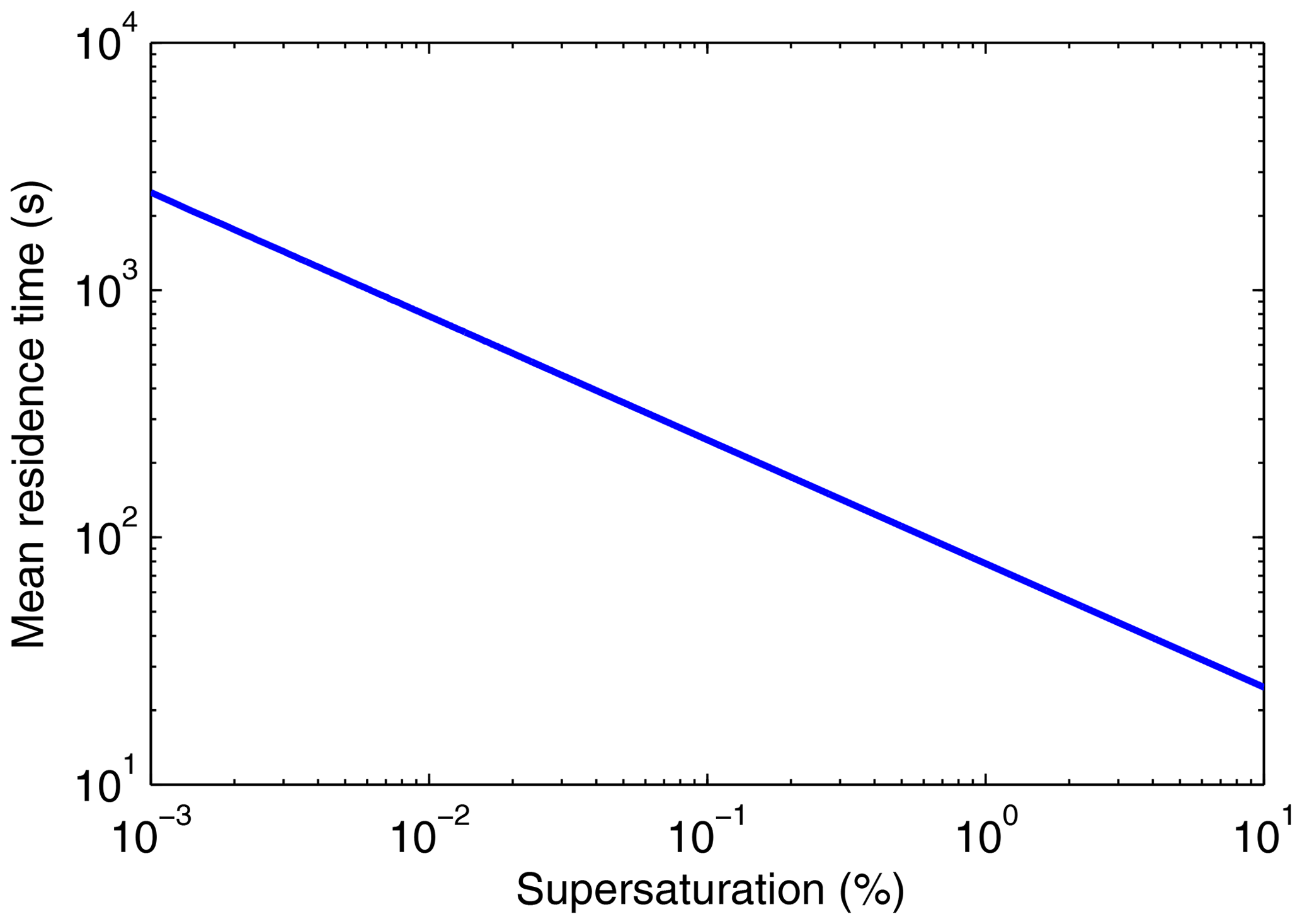
This follows from using Eq. (52) for F_sed and Eq. (29) for $\stackrel{\mathrm{‾}}{r^{\mathrm{2}}}$. The mean residence time in this case depends upon the chamber height, the Stokes fall speed coefficient, and the supersaturation. Figure 10 shows $\stackrel{\mathrm{‾}}{\mathit{\tau }}$ versus the supersaturation for h=1 m. Figure 6 shows that the range of nominal mean supersaturations inferred from the measured moments is 0.008 % to 0.8 %. Figure 10 indicates that $\stackrel{\mathrm{‾}}{\mathit{\tau }}$ decreases from about 900 to 90 s over this range of actual supersaturations.

We noted in Sect. 6 that the actual fall speed parameter, $k{{}^{\prime }}_{\mathrm{1}}$, is unknown. However, it could be determined from measurements of $\stackrel{\mathrm{‾}}{\mathit{\tau }}$, $\stackrel{\mathrm{‾}}{r^{\mathrm{2}}}$, and N by using Eqs. (52) and (54):

$$k_{\mathrm{1}}^{\prime }={\displaystyle \frac{hN}{\stackrel{\mathrm{‾}}{\mathit{\tau }}\stackrel{\mathrm{‾}}{r^{\mathrm{2}}}}}.$$

Figure 10 Mean droplet residence time versus supersaturation for h=1 m as given by Eq. (54).

To derive the PDF of droplet residence times, R(τ), we start with the probability for a droplet of radius r to fall out in a small time interval, dt, which we derived in Sect. 2.3, then use r²=2ξt to obtain

$${\displaystyle \frac{k_{\mathrm{1}}{r}^{\mathrm{2}}}{h}}\mathrm{d}t={\displaystyle \frac{\mathrm{2}{k}_{\mathrm{1}}\mathit{\xi }}{h}}t\mathrm{d}t\equiv bt\mathrm{d}t.$$

This means that during a time interval dt, a fraction b t dt of the droplets falls out. If n(t) is the number of droplets injected at t=0 that remain at time t, then

$${\displaystyle \frac{\mathrm{d}n}{\mathrm{d}t}}=-btn,$$

which has the solution $n\left(t\right)=n\left(\mathrm{0}\right)\exp (-b{t}^{\mathrm{2}}/\mathrm{2}).$ The distribution of droplet residence times is therefore dn(t)∕dt, which we normalize to obtain the PDF of droplet residence times,

$$\begin{array}{}\text{(56)}& R\left(\mathit{\tau }\right)=b\mathit{\tau }\exp (-b{\mathit{\tau }}^{\mathrm{2}}/\mathrm{2}).\end{array}$$

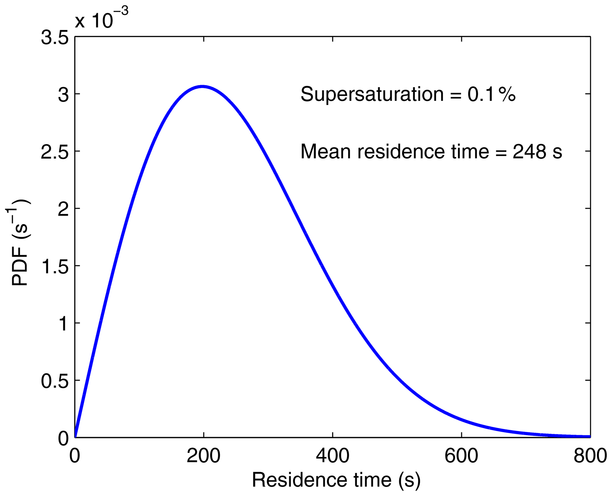
We verified that the mean droplet residence time obtained from Eq. (56) agrees with Eq. (54). Figure 11 displays the PDF of droplet residence times, R(τ), for 0.1 % supersaturation and h=1 m. In Fig. 2 (in Sect. 3), we compared R(τ) from a Monte Carlo method and R(τ) from Eq. (56) for 0.1 % supersaturation.

Figure 11 PDF of droplet residence times for 0.1 % supersaturation and h=1 m as given by Eq. (56).

8.5 Condensation rate

To derive the condensation rate of a population of droplets, d$\stackrel{\mathrm{‾}}{q}/\mathrm{d}t$ (mass of water condensed per mass of dry air per unit time), start with the condensation rate for a single droplet,

$${\displaystyle \frac{\mathrm{d}m}{\mathrm{d}t}}={\mathit{\rho }}_L\mathrm{4}\mathit{\pi }\mathit{\xi }r,$$

where we used $\mathrm{d}r/\mathrm{d}t=\mathit{\xi }/r$. Then

$$\begin{array}{}\text{(57)}& \begin{array}{rl}{\displaystyle \frac{\mathrm{d}\stackrel{\mathrm{‾}}{q}}{\mathrm{d}t}}& =\underset{\mathrm{0}}{\overset{\mathrm{\infty }}{\int }}{\displaystyle \frac{\mathrm{d}m}{\mathrm{d}t}}v\left(r\right)\mathrm{d}r=D\underset{\mathrm{0}}{\overset{\mathrm{\infty }}{\int }}{\mathit{\rho }}_L\mathrm{4}\mathit{\pi }\mathit{\xi }{r}^{\mathrm{2}}\exp (-C{r}^{\mathrm{4}}/\mathrm{4})\mathrm{d}r\\ & ={\displaystyle \frac{{\mathit{\rho }}_L\mathrm{4}\mathit{\pi }\mathit{\xi }}{\mathit{\rho }}}N{\displaystyle \frac{\sqrt{\mathrm{2}}\mathrm{\Gamma }(\mathrm{3}/\mathrm{4})}{\sqrt{\mathit{\pi }}{C}^{\mathrm{1}/\mathrm{4}}}}.\end{array}\end{array}$$

One can easily verify that d$\stackrel{\mathrm{‾}}{q}/\mathrm{d}t=P/\left(\mathit{\rho }h\right)$ using P from Eq. (53) and $\stackrel{\mathrm{‾}}{r^{\mathrm{5}}}$ from Eq. (41), along with $C\equiv k_{\mathrm{1}}/\left(\mathit{\xi }h\right)$ and $\mathrm{\Gamma }(\mathrm{7}/\mathrm{4})/\mathrm{\Gamma }(\mathrm{3}/\mathrm{4})=\mathrm{3}/\mathrm{4}$. An equivalent form that is not specific to a particular DSD was derived by (Korolev and Mazin, 2003):

$$\begin{array}{}\text{(58)}& \begin{array}{rl}{\displaystyle \frac{\mathrm{d}\stackrel{\mathrm{‾}}{q}}{\mathrm{d}t}}& ={\displaystyle \frac{N}{\mathit{\rho }}}\underset{\mathrm{0}}{\overset{\mathrm{\infty }}{\int }}{\displaystyle \frac{\mathrm{d}m}{\mathrm{d}t}}p\left(r\right)\mathrm{d}r={\displaystyle \frac{N{\mathit{\rho }}_L\mathrm{4}\mathit{\pi }\mathit{\xi }}{\mathit{\rho }}}\underset{\mathrm{0}}{\overset{\mathrm{\infty }}{\int }}rp\left(r\right)\mathrm{d}r\\ & ={\displaystyle \frac{{\mathit{\rho }}_L\mathrm{4}\mathit{\pi }\mathit{\xi }}{\mathit{\rho }}}N\stackrel{\mathrm{‾}}{r}.\end{array}\end{array}$$

One can use Eq. (26) to show that Eq. (57) is equal to Eq. (58).

9 Conclusions

In a laboratory cloud chamber, such as the Π chamber at Michigan Technological University, it is possible to produce Rayleigh–Bénard convection by applying an unstable temperature gradient between the top and bottom water-saturated surfaces of the chamber. Supersaturation is produced by isobaric mixing within the turbulent flow. When aerosols (cloud condensation nuclei) are injected at a constant rate, an equilibrium state is achieved in which the rate of droplet activation is balanced by the rate of droplet loss. After a droplet is activated, it continues to grow by condensation until it falls out (i.e., contacts the bottom surface).

Because supersaturation is difficult to measure when cloud droplets are present, it has not been generally possible to determine the magnitudes of the mean supersaturation and the supersaturation fluctuations in the Pi chamber under cloudy conditions. Therefore, it also has not been generally possible to directly determine the relative contributions of mean and fluctuating supersaturation to the measured droplet PDFs.

We derived analytic PDFs of droplet radius and squared radius for conditions that could occur in a turbulent cloud chamber in which there is uniform supersaturation, droplet curvature and solute effects on droplet growth are negligible, and a balance exists between droplet formation (activation) and loss (due to fallout). The loss rate due to fallout is based on three assumptions. (1) The droplets are well-mixed by turbulence, in which case the z coordinate of each droplet is a random variable. (2) When a droplet becomes sufficiently close to the lower boundary, the droplet's terminal velocity determines its probability of fallout per unit time. (3) A droplet's terminal velocity is proportional to its radius squared. Given the chamber height and the droplet fall speed's dependence on squared radius, the analytic PDFs are determined by the supersaturation alone.

It should be emphasized that it is only the supersaturation that directly determines the droplet radius PDF. A cloud chamber undergoing Rayleigh–Bénard convection is analogous to an ascending parcel: in both cases a forcing process continually increases the supersaturation, while droplet growth decreases it. For an ascending parcel, the forcing process is adiabatic cooling, while for a cloud chamber, it is turbulent fluxes of sensible heat and water vapor from the walls. In both cases, the timescale for condensation to decrease supersaturation is the phase relaxation timescale, which depends inversely on droplet number concentration and mean radius (Squires, 1952). The quasi-steady supersaturation is determined by a balance between these two processes.

We demonstrated how the equilibrium radius distribution is realized by using a Monte Carlo method and compared the results to some of those that were obtained analytically. A notable feature is the wide PDF of droplet residence times. This PDF determines the width of the DSD when there is uniform supersaturation: all droplets grow at the same rate, so the greater a droplet's residence time, the larger it gets and the more it contributes to the large-droplet tail of the PDF.

From the analytic equilibrium PDFs of radius and of squared radius, we obtained expressions for the median and mode radii. We also derived the first five moments of the radius from the analytic equilibrium PDFs, including moments for truncated DSDs (those with positive lower limits). We used statistics from a set of measured DSDs to check for consistency with the analytic PDF. The droplet number concentrations of the measured DSDs ranged from 14 to 3000 cm⁻³. We found consistency between theoretical and measured moments, but only when the truncation radius of the measured DSDs was taken into account. Because the theoretical moments depend only on the supersaturation once the chamber height, Stokes' fall speed parameter, and truncation radius are specified, consistency between theoretical and measured moments allows us to infer the mean supersaturations that would produce the measured DSDs in the absence of supersaturation fluctuations. From the mean radius, mean squared radius, and mean cubed radius for 11 measured DSDs, the inferred mean supersaturations ranged from 0.008 % to 0.6 %. We found that neglecting the curvature and solute terms in the droplet growth rate equation can sometimes affect the inferred supersaturations. For a given droplet radius, the inferred supersaturation is larger with solute and curvature terms included. Calculations with a Monte Carlo model with solute and curvature terms included suggest that for the aerosols injected into the cloud chamber, a measured DSD (r>2.5 µm only) with a mean radius of about 4.4 µm or larger could have been activated and grown with a fixed supersaturation of 0.055 %. This excludes the DSDs with the five smallest mean radii. To produce these DSDs, there must have been supersaturation fluctuations somewhere in the cloud chamber that exceeded the critical supersaturation for at least the larger injected aerosols.

We found that accounting for the truncation radius of the measured DSDs is particularly important when comparing the theoretical and measured relative dispersions of the droplet radius. We showed that the monotonic decrease in the measured relative dispersion reported by Chandrakar et al. (2018a, c) is due to not taking truncation into account and that when truncation of the DSD is taken into account, our theoretical values match the measured values.

Finally, we presented some additional quantities derived from the analytic DSD: droplet sedimentation flux, precipitation flux, and condensation rate.