Inverse modeling of SO₂ and NO_x emissions over China using multisensor satellite data – Part 1: Formulation and sensitivity analysis

SO₂ and NO₂ observations from the Ozone Mapping and Profiler Suite (OMPS) sensor are used for the first time in conjunction with the GEOS-Chem adjoint model to optimize both SO₂ and NO_x emission estimates over China for October 2013. Separate and joint (simultaneous) optimizations of SO₂ and NO₂ emissions are both conducted and compared. Posterior emissions, compared to the prior, yield improvements in simulating columnar SO₂ and NO₂, in comparison to measurements from the Ozone Monitoring Instrument (OMI) and OMPS. The posterior SO₂ and NO_x emissions from separate inversions are 748 Gg S and 672 Gg N, which are 36 % and 6 % smaller than prior MIX emissions (valid for 2010), respectively. In spite of the large reduction of SO₂ emissions over the North China Plain, the simulated sulfate–nitrate–ammonium aerosol optical depth (AOD) only decrease slightly, which can be attributed to (a) nitrate rather than sulfate as the dominant contributor to AOD and (b) replacement of ammonium sulfate with ammonium nitrate as SO₂ emissions are reduced. For joint inversions, both data quality control and the weight given to SO₂ relative to NO₂ observations can affect the spatial distributions of the posterior emissions. When the latter is properly balanced, the posterior emissions from assimilating OMPS SO₂ and NO₂ jointly yield a difference of −3 % to 15 % with respect to the separate assimilations for total anthropogenic SO₂ emissions and ±2 % for total anthropogenic NO_x emissions; but the differences can be up to 100 % for SO₂ and 40 % for NO₂ in some grid cells. Improvements on SO₂ and NO₂ simulations from the joint inversions are overall consistent with those from separate inversions. Moreover, the joint assimilations save ∼ 50 % of the computational time compared to assimilating SO₂ and NO₂ separately in a sequential manner of computation. The sensitivity analysis shows that a perturbation of NH₃ to 50 % (20 %) of the prior emission inventory can (a) have a negligible impact on the separate SO₂ inversion but can lead to a decrease in posterior SO₂ emissions over China by −2.4 % (−7.0 %) in total and up to −9.0 % (−27.7 %) in some grid cells in the joint inversion with NO₂ and (b) yield posterior NO_x emission decreases over China by −0.7 % (−2.8 %) for the separate NO₂ inversion and by −2.7 % (−5.3 %) in total and up to −15.2 % (−29.4 %) in some grid cells for the joint inversion. The large reduction of SO₂ between 2010 and 2013, however, only leads to ∼ 10 % decrease in AOD regionally; reducing surface aerosol concentration requires the reduction of emissions of NH₃ as well.

1 Introduction

Both SO₂ and NO₂ in the atmosphere have adverse impacts on human health and can affect radiative forcing that leads to climate change. Not only do they cause inflammation and irritation of humans' respiratory system, but they also react with other species to form sulfate and nitrate aerosols (Seinfeld and Pandis, 2016), which subsequently can lead to or exacerbate respiratory and cardiovascular diseases (Lim et al., 2012). Sulfate and nitrate account for the largest mass of anthropogenic aerosols, which contributed to ∼ 3 million premature deaths worldwide in 2010 (Lelieveld et al., 2015). In addition to the health impacts, anthropogenic sulfate and nitrate particles are estimated to have caused −0.4 and −0.15 W m⁻² radiative forcing, respectively, on a global scale between 1750 and 2011 through the scattering of solar radiation and the modification of cloud microphysical properties (Myhre et al., 2013).

Satellite-derived global distributions of SO₂ and NO₂ vertical column densities (VCDs) have been used to study the aforementioned impacts of SO₂ and NO₂ on atmospheric composition, climate change, and human health. In particular, since SO₂ and NO₂ VCDs are, to a first order, linearly related to SO₂ and NO_x emissions (Calkins et al., 2016), they can be used to update bottom-up emission inventories that have large uncertainties and a temporal lag often of at least 1 year (Liu et al., 2018). Of particular interest for this study is China, which has large SO₂ and NO_x emissions from anthropogenic sources (coal-fired power plants, industry, transportation, and residential activity). Moreover, China has seen a 62 % reduction in anthropogenic SO₂ emissions and a 17 % reduction of anthropogenic NO_x emissions on average from 2010 to 2017 (Zheng et al., 2018) due to the implementation of emission control policies, and these changes vary by regions, cities (Liu et al., 2016), and sectoral sources (Zheng et al., 2018). The reduction of SO₂ emissions mainly occurred in the coal-fired power plants and industries, while the decrease in NO_x emissions was largely ascribed to coal-fired power plants (Zheng et al., 2018). Noticeable uncertainties larger than 30 % for both anthropogenic SO₂ and NO_x in 2010 over China were documented (Li et al., 2017b) and can be larger at the regional scale due to the uncertainty of activity rates, emission factors, and spatial proxies, which are used in the bottom-up approach (Janssens-Maenhout et al., 2015). The uncertainty is large and can be compounded by possible discrepancies caused by the temporal lag of bottom-up emission inventories and the rapid changes in emissions over time.

Several methods have been developed to update SO₂ and NO_x emissions using satellite VCD retrievals of SO₂ and NO₂, which have global coverage and allow near-real-time access. The mass balance method, which scales prior emissions by the ratios of observed VCDs to chemistry transport model (CTM) counterparts, was applied to SO₂ retrievals from the SCanning Imaging Absorption spectroMeter for Atmospheric CHartographY (SCIAMACHY) and Ozone Monitoring Instrument (OMI) (Lee et al., 2011; Koukouli et al., 2018) and to NO₂ from the Global Ozone Monitoring Experiment (GOME) and OMI (Martin et al., 2003; Lamsal et al., 2010) to estimate SO₂ and NO_x emissions, respectively. Lamsal et al. (2011) simulated the sensitivity of VCDs to emissions (the finite-difference mass balance approach) using a CTM, which was applied to OMI NO₂ retrievals to estimate NO_x emissions. SO₂ VCD retrievals from GOME, GOME-2, SCIAMACHY, and the Ozone Mapping and Profiler Suite (OMPS) were used to estimate point sources through linear regression between VCDs and emissions or function fitting, although the method can only detect about half of the total anthropogenic SO₂ emissions (Li et al., 2017a; Zhang et al., 2017; Fioletov et al., 2013, 2016). With explicit considerations of chemistry, transport, and deposition, the four-dimension variational data assimilation (4D-Var) approach was applied to estimate emissions using SO₂ data from OMI (Wang et al., 2016; Qu et al., 2019a) and NO₂ data from SCIAMACHY, GOME-2, and OMI (Kurokawa et al., 2009; Qu et al., 2017; Kong et al., 2019). The 4D-Var posterior has a smaller root mean square error than the mass balance posterior, especially in the conditions when the initial guess and true emissions have different spatial patterns (Qu et al., 2017); this is because the spatial extent of source influences on modeled column concentrations (Turner et al., 2012) is only indirectly and partially accounted for in the mass balance approach. Cooper et al. (2017), however, showed that the iterative finite-difference mass balance approach has a similar normalized mean error value to the 4D-Var approach for global-scale models with coarse resolution when synthetic NO₂ columns observations are used to constrain NO_x emissions. To combine the strengths of the 4D-Var and mass balance approaches, Qu et al. (2017) further introduced a hybrid 4D-Var-mass-balance approach, which can better capture trends and spatial variability of NO_x emissions than the mass balance approach and save significant computational resources when applied to constrain monthly NO_x emissions for multiple years. Other data assimilation approaches including the ensemble Kalman filter method (Miyazaki et al., 2012, 2017) and the Daily Emission estimates Constrained by Satellite Observation (DECSO) algorithm (Mijling and van der A, 2012; Ding et al., 2015) have also been used to constrain NO_x emissions.

Here, we focus on the development and feasibility for joint 4D-Var assimilation of satellite-based SO₂ and NO₂ data to optimize SO₂ and NO_x emission strengths simultaneously. Specifically, this study aims to conduct 4D-Var assimilation of VCDs of SO₂ and NO₂ from OMPS to constrain SO₂ and NO_x emissions over China using the GEOS-Chem 4D-Var inverse modeling framework. In our companion study (Wang et al., 2020), we develop approaches to downscaling the optimized emission inventories for improving air quality predictions. Despite their numerous applications for top-down estimates of SO₂ and NO_x emissions in the past two decades, GOME and SCIAMACHY stopped providing data in 2004 and 2012, respectively, while OMI has been suffering from a row anomaly that leads to much less spatial coverage and larger data uncertainty (Schenkeveld et al., 2017). Hence, it is important to study the potential of next-generation sensors such as OMPS toward continuously monitoring the change in SO₂ and NO_x emissions and their atmospheric loadings. Two OMPS sensors on board the Suomi National Polar-orbiting Partnership (Suomi NPP) and NOAA-20 were launched in 2011 and 2018, respectively, and the third one is expected to be launched in 2020. As OMPS will continue to provide SO₂ and NO₂ retrievals in the next two decades, this study, for the first time, seeks to provide a critical assessment of the extent to which the OMPS observations improve emission estimates and air quality forecast at the regional scale.

The novelty of this study lies not only in the first application of OMPS SO₂ and NO₂ retrievals to constrain emissions using the 4D-Var technique but also in the deployment of OMI data to assess the GEOS-Chem simulation with posterior emissions, thereby studying the degree to which OMPS and OMI retrievals, despite their difference in sensor characteristics and inversion techniques, can provide consistent constraints for the model improvement. Qu et al. (2019a) showed that posterior SO₂ emissions derived from different OMI SO₂ products vary in strength and have consistent trend signs. Our study here using OMPS thus examines an important issue, which is whether or not there would be any artificial trends in our climate data record of atmospheric SO₂ and NO₂ due to the transition of satellite sensors (Wang and Wang, 2020). Our study is also different from past studies (Wang et al., 2016; Qu et al., 2017, 2019a, b) that have applied the 4D-Var technique to OMI data with the GEOS-Chem adjoint model but did not include evaluation with independent satellite data. Qu et al. (2019b) showed joint inversion using OMI SO₂ and NO₂ benefits from simultaneous adjustment of OH and O₃ concentrations, which supports assimilating OMPS SO₂ and NO₂ observations simultaneously in this study. Additionally, considering that the uncertainty of NH₃ emission inventories is up to 153 % over China (Kurokawa et al., 2013) and NH₃ emissions are not constrained in our inversions, we also explore issues related to the covariation among species that appear to be independent but indeed are connected through chemical processes and analyze the differences in responses of emissions and aerosols to NH₃ emissions uncertainty between joint and single-species assimilations. Finally, this paper also provides the foundation for the Part 2 investigation (Wang et al., 2020) in which we develop various downscaling methods to illustrate that optimized emission, albeit with coarse resolution inherent from OMPS data, can be used to improve the air quality forecast at a resolution much finer than OMPS pixel size.

We describe OMPS and OMI data in Sect. 2. The GEOS-Chem model and its adjoint as well as the design of numerical experiments are presented in Sect. 3. Results of case studies for October 2013 are provided in Sect. 4. Section 5 consists of discussion and conclusions.

2 Data

2.1 OMPS data as constraints

We use OMPS level-2 SO₂ and NO₂ tropospheric VCDs in October 2013 as constraints to optimize SO₂ and NO_x emissions over China. The OMPS nadir mapper on board the Suomi NPP satellite, launched in November 2011, observes hyperspectral solar irradiance and earthshine radiance at 300–380 nm (Flynn et al., 2014). With 35 detectors of 50 km×50 km nominal pixel size in the cross-track direction, OMPS has a swath of 2800 km flying across the Equator at 13:30 local time ascending at the sunlit side of the Earth surface and providing global coverage daily. Both SO₂ and NO₂ are retrieved through the direct vertical column fitting (DVCF) algorithm with SO₂ and NO₂ atmospheric profile information from GEOS-Chem simulations and have a retrieval precision of 0.2 and 0.011 DU, respectively, which are estimated from the standard background (a clean region that is far from emission sources) retrievals (Yang et al., 2013, 2014). These precision values can be used as the observation error in the cost function of data assimilation. However, we should notice that the estimated observation (retrieval) errors only represent the observation error distribution of the products as a whole; they cannot represent the observation error distribution for every pixel, because the pixel-level error is amenable to spatiotemporal change in cloud fraction, satellite observation geometry, aerosol impacts, etc. In theory, if the uncertainties could be analytically described at the pixel level, they would be directly applied to improve the satellite product in the first place.

Only pixels with both solar zenith angle (SZA) and view zenith angle (VZA) less than 75^∘ are used, as larger SZA or VZA results in longer light path length and consequently less information content and lower data quality for retrieving the change in SO₂ or NO₂ loadings in the planetary boundary layer (PBL) where the two trace gases from anthropogenic sources mainly concentrate. We also remove the pixels with radiative cloud fraction (RCF) larger than 0.2 for SO₂ and 0.3 for NO₂ as a trade-off between the data amount and cloud impacts. Considering their large uncertainty, OMPS SO₂ retrievals in the grid cell where the prior simulation is less than 0.1 DU will not be used, except in quality control (QC) sensitivity analysis experiments.

2.2 OMI data for assessment

OMI level-3 SO₂ and NO₂ tropospheric VCDs at a spatial resolution of $\mathrm{0.25}{}^{\circ }\times \mathrm{0.25}{}^{\circ }$ from NASA are used for evaluating the model results. OMI is a UV–visible hyperspectral sensor that observes solar irradiance and earthshine radiance at 300–500 nm. The swath of OMI is 2600 km, consisting of 60 detectors with the nominal pixel size of 13 km×24 km at nadir. OMI flies across the Equator in the ascending node at 13:45 local time, which is very close to the 13:30 local time for OMPS. Due to row anomaly (Schenkeveld et al., 2017), OMI takes more than 1 d to provide global coverage. The level-3 product is derived from the level-2 product; the latter is retrieved through the principal component analysis (PCA) algorithm with a fixed air mass factor (AMF) assumption for SO₂ (Li et al., 2013) and variation of the differential optical absorption spectroscopy (DOAS) algorithm for NO₂ (Krotkov et al., 2017; Marchenko et al., 2015), with a precision of 0.5 DU (Li et al., 2013) and 0.017 DU (Krotkov et al., 2017), respectively. In the level-3 product, pixels affected by row anomaly are removed. For SO₂, only the pixel with the shortest light path, SZA less than 70^∘ , RCF less than 0.2, and detector number in the range of 2 to 59 (numbering sequences starting at 1) is retained in a $\mathrm{0.25}{}^{\circ }\times \mathrm{0.25}{}^{\circ }$ grid cell and then corrected with a new AMF based on GEOS-Chem SO₂ profile simulation (Leonard, 2017). For the OMI level-2 NO₂ product, the AMF calculation is based on Global Modeling Initiative NO₂ profile simulation (Krotkov et al., 2017), and all pixels with SZA less than 85^∘, terrain reflectivity less than 0.3, and RCF less than 0.3 are averaged in a $\mathrm{0.25}{}^{\circ }\times \mathrm{0.25}{}^{\circ }$ grid cell weighted by the overlapping area of the grid cell and pixel to form the level-3 product (Bucsela et al., 2016). In the assessments, OMI observations are averaged in a $\mathrm{2}{}^{\circ }\times \mathrm{2.5}{}^{\circ }$ model grid cell, and model simulations are sampled by OMI observational time.

3 Method

3.1 GEOS-Chem and its adjoint

GEOS-Chem is a 3-D chemistry transport model driven by emissions and GEOS-FP meteorological fields. The secondary sulfate–nitrate–ammonium aerosol formation in the model is introduced by Park et al. (2004). Both aerosols and gases are removed by wet deposition, including washout and rainout from large-scale or convective precipitation (Liu et al., 2001) and the dry deposition following a resistance-in-series scheme with aerodynamic resistance and boundary resistance calculated from GEOS-FP meteorological field and surface resistances based largely on a canopy model (Wang et al., 1998; Wesely, 1989). Anthropogenic SO₂, NO_x, and NH₃ emissions used over East Asia are the mosaic emission inventory (MIX) (Li et al., 2017b) for year 2010. SO₂ and NO₂ VCDs are simulated at $\mathrm{2}{}^{\circ }\times \mathrm{2.5}{}^{\circ }$ resolution with 47 vertical layers using both the prior and posterior emission inventories to compare with OMI retrievals.

The GEOS-Chem adjoint model is a tool for efficiently calculating the sensitivity of a scalar cost function with respect to large numbers of model parameters simultaneously such as emissions (Henze et al., 2007). In this study, the cost function is defined as Eq. (1).

$$\begin{array}{}\text{(1)}& \begin{array}{rl}\mathrm{J}\left(\mathit{\sigma }\right)=& \mathit{\gamma }{\displaystyle \frac{\mathrm{1}}{\mathrm{2}}}{\left[{\mathrm{H}}_{{\mathrm{SO}}_{\mathrm{2}}}\left(\mathrm{M}\left(\mathit{\sigma }\right)\right)-{\mathit{c}}_{{\mathrm{SO}}_{\mathrm{2}}}\right]}^{\mathrm{T}}\\ & {\mathbf{S}}_{{\mathrm{SO}}_{\mathrm{2}}}^{-\mathrm{1}}\left[{\mathrm{H}}_{{\mathrm{SO}}_{\mathrm{2}}}\left(\mathrm{M}\left(\mathit{\sigma }\right)\right)-{\mathit{c}}_{{\mathrm{SO}}_{\mathrm{2}}}\right]\\ & +{\displaystyle \frac{\mathrm{1}}{\mathrm{2}}}{\left[{\mathrm{H}}_{{\mathrm{NO}}_{\mathrm{2}}}\left(\mathrm{M}\left(\mathit{\sigma }\right)\right)-{\mathit{c}}_{{\mathrm{NO}}_{\mathrm{2}}}\right]}^{\mathrm{T}}\\ & {\mathbf{S}}_{{\mathrm{NO}}_{\mathrm{2}}}^{-\mathrm{1}}\left[{\mathrm{H}}_{{\mathrm{NO}}_{\mathrm{2}}}\left(\mathrm{M}\left(\mathit{\sigma }\right)\right)-{\mathit{c}}_{{\mathrm{NO}}_{\mathrm{2}}}\right]\\ & +{\displaystyle \frac{\mathrm{1}}{\mathrm{2}}}{\left[\mathit{\sigma }-{\mathit{\sigma }}_{\mathrm{a}}\right]}^{\mathrm{T}}{\mathbf{S}}_{\mathrm{a}}^{-\mathrm{1}}\left[\mathit{\sigma }-{\mathit{\sigma }}_{\mathrm{a}}\right]\end{array}\end{array}$$

where σ is a state vector, consisting of $\ln (E_i/E_{\text{a},i})$, and E_i and E_a,i are the ith element in E and E_a, respectively. E is a vector in which SO₂ and NO_x emissions are ordered by GEOS-Chem model grid cell and by species, and E_a is a prior estimate of it. ${\mathit{c}}_{{\mathrm{SO}}_{\mathrm{2}}}$ and ${\mathit{c}}_{{\mathrm{NO}}_{\mathrm{2}}}$ are vectors of OMPS SO₂ and NO₂ tropospheric VCDs, respectively. ${\mathbf{S}}_{{\mathrm{SO}}_{\mathrm{2}}}$ and ${\mathbf{S}}_{{\mathrm{NO}}_{\mathrm{2}}}$ are observation error covariance matrixes for SO₂ and NO₂ and are assumed to be diagonal, which means observational errors are uncorrelated. M is the GEOS-Chem model that simulates the relationship between SO₂ and NO₂ concentrations in the atmosphere and the emission factors. H${}_{{\mathrm{SO}}_{\mathrm{2}}}$ and H${}_{{\mathrm{NO}}_{\mathrm{2}}}$ are observation operators which map GEOS-Chem simulations of SO₂ and NO₂ to the observational space, respectively. σ_a is the prior estimate of σ, and S_a is the error covariance matrix for σ_a. S_a is assumed to be diagonal with a relative error of 50 % for SO₂ and 100 % for NO_x as used in Xu et al. (2013). γ is a parameter we introduce to balance the importance of the SO₂ observation term (first term on the right side of Eq. 1) and NO₂ observational term (second term on the right side of Eq. 1), given both the different sizes and observation errors of these two observation datasets.

OMPS SO₂ and NO₂ tropospheric VCDs are directly compared to GEOS-Chem tropospheric VCDs of SO₂ (H${}_{{\mathrm{SO}}_{\mathrm{2}}}\left(\mathrm{M}\left(\mathit{\sigma }\right)\right)$ in Eq. 1) and NO₂ (${\mathrm{H}}_{{\mathrm{NO}}_{\mathrm{2}}}\left(\mathrm{M}\left(\mathit{\sigma }\right)\right)$ in Eq. 1). Retrieving SO₂ and NO₂ tropospheric VCDs from the satellite requires assumptions regarding SO₂ and NO₂ vertical profiles, as the sensitivity of the radiance observed by satellite sensors to the changes in SO₂ or NO₂ loadings is a function of plume height. If the vertical profile assumptions in the retrieval process are inconsistent with the GEOS-Chem simulations, the inconsistency partly contributes to the difference between the GEOS-Chem simulations and the OMPS retrievals (H${}_{{\mathrm{SO}}_{\mathrm{2}}}\left(\mathrm{M}\left(\mathit{\sigma }\right)\right)-{\mathit{c}}_{{\mathrm{SO}}_{\mathrm{2}}}$ or ${\mathrm{H}}_{{\mathrm{NO}}_{\mathrm{2}}}\left(\mathrm{M}\left(\mathit{\sigma }\right)\right)-{\mathit{c}}_{{\mathrm{NO}}_{\mathrm{2}}}$). In this study, OMPS SO₂ and NO₂ tropospheric VCDs are retrieved using the shape of vertical profiles from GEOS-Chem simulations (Yang et al., 2013, 2014), but the differences in model version, simulation year, and emission inventory still exist. These differences still can lead to the differences in vertical profiles, hence partly contributing to the difference between the GEOS-Chem simulations and the OMPS retrievals. The vertical profile differences can lead to a mean bias of −6.8 % overall at the pixel level (Fig. S1) and −7.5 % (Fig. S2) for OMPS SO₂ and NO₂ retrievals, respectively. And we shall discuss the impacts of these biases on emission inverse modeling in Sect. 4.1.1.

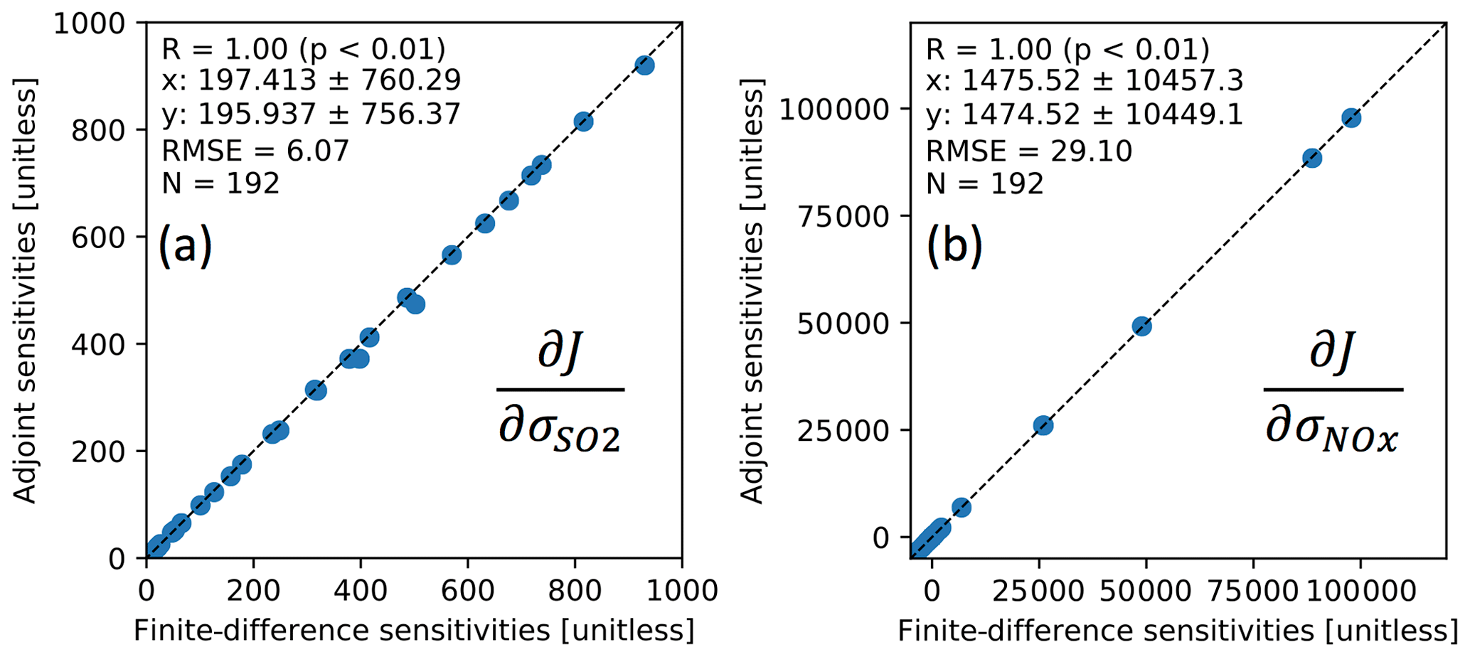
Figure 1 Validation of adjoint model sensitivity through comparison to centered finite-difference results for a 3 d simulation. Shown here is the sensitivity of the column cost function (penalty term is not included, and horizontal transport is turned off) with respect to the logarithm of anthropogenic SO₂ (a) and NO_x (b) emission scale factors: the 1 : 1 line (dotted), number of grid columns (N), root mean squared error (RMSE), and correlation coefficient (R), and means and standard deviations of finite-difference sensitivity and adjoint sensitivity (x and y).

In the optimization formulation, the forward model errors are also considered as part of the observation error term. However, while several ways to construct model error covariance matrix exist, including the Hollingsworth–Lönnberg (Hollingsworth and Lönnberg, 1986) and NMC (Bannister, 2008) methods, their application for offline CTM model error characterization deserves a separate study. The Hollingsworth method extracts observation error variance (including forward model error) from (observation–background) covariance statistics with the assumptions that observation error is spatially uncorrelated, background error is spatially correlated as a function of distance, and observation error and background error are uncorrelated. The assumption that background error is spatially correlated as a function of distance only is suitable for the meteorological fields that vary smoothly, but for chemical species, emissions also contribute significantly to model errors and emissions may not be spatially correlated. The NMC method is normally applied to weather forecast models or online-coupled weather–chemistry models (Benedetti and Fisher, 2007). Offline CTMs such as GEOS-Chem use the meteorological reanalysis, and therefore NMC is not applicable here to quantify the CTM's transport error. Consequently, the CTM's transport errors are neglected in the past emission optimization work (Wang et al., 2016) and are adopted in this study. Admittedly, this simplification should be studied in the future together with the evaluation and developments of methods to characterize offline CTM errors.

We developed the observation operators for OMPS SO₂ and NO₂, and the validations are shown in Fig. 1. The sensitivities of the cost function with respect to anthropogenic SO₂ and NO_x emissions from the adjoint model are consistent with the sensitivities calculated through the finite-difference approach. Hence, Fig. 1 confirms the correctness of the new observation operators integrated into the GEOS-Chem adjoint model.

To optimize the emission inventories, σ is adjusted iteratively until the cost function is minimized. The minimization is conducted with the L-BFGS-B algorithm (Byrd et al., 1995), which utilizes the sensitivity of the cost function with respect to σ that is calculated by the GEOS-Chem adjoint model. The minimization process halts when the difference in the cost function between two consecutive iterations is less than 3 %. This selection is to expedite the computation while still maintaining the similar accuracy for the optimization; further tests show that more iterations (after < 3 % reduction of cost function) do not yield a discernible difference in the cost function values (Fig. S3) and optimization results (Tables S1 and S2).

3.2 Experiment design

Several elements play a role in the inverse modeling of emissions, including data quality control, balancing the spatial distributions of observational frequencies for the same species, balancing the observation contributions from different species, and uncertainties in the NH₃ emission inventory (because NH₃ has impacts on SO₂ and NO₂ lifetimes). To investigate the impacts of these factors on the posterior emissions, we design a set of experiments as summarized in Tables 1 and 2. All these experiments use OMPS SO₂ and NO₂ retrievals to optimize corresponding emissions over China in October 2013 at a horizontal resolution of $\mathrm{2}{}^{\circ }\times \mathrm{2.5}{}^{\circ }$. Although finer-resolution options such as $\mathrm{0.5}{}^{\circ }\times \mathrm{0.625}{}^{\circ }$ or $\mathrm{0.25}{}^{\circ }\times \mathrm{0.3125}{}^{\circ }$ are available for China, the $\mathrm{2}{}^{\circ }\times \mathrm{2.5}{}^{\circ }$ resolution is selected for two reasons: (1) it saves computational time and (2) the coarse resolution of OMPS retrievals (50 km × 50 km at nadir and 190 km × 50 km at edges) has no first-order information to resolve the emissions at a fine resolution of $\mathrm{0.5}{}^{\circ }\times \mathrm{0.625}{}^{\circ }$ or $\mathrm{0.25}{}^{\circ }\times \mathrm{0.3125}{}^{\circ }$. In Part 2 (Wang et al., 2020) of this study, we develop downscaling tools for regional air quality modeling. Indeed, one of the goals of the two-part investigation is to illustrate how OMPS data could be used to improve the air quality forecast at a resolution much finer than OMPS pixel size.

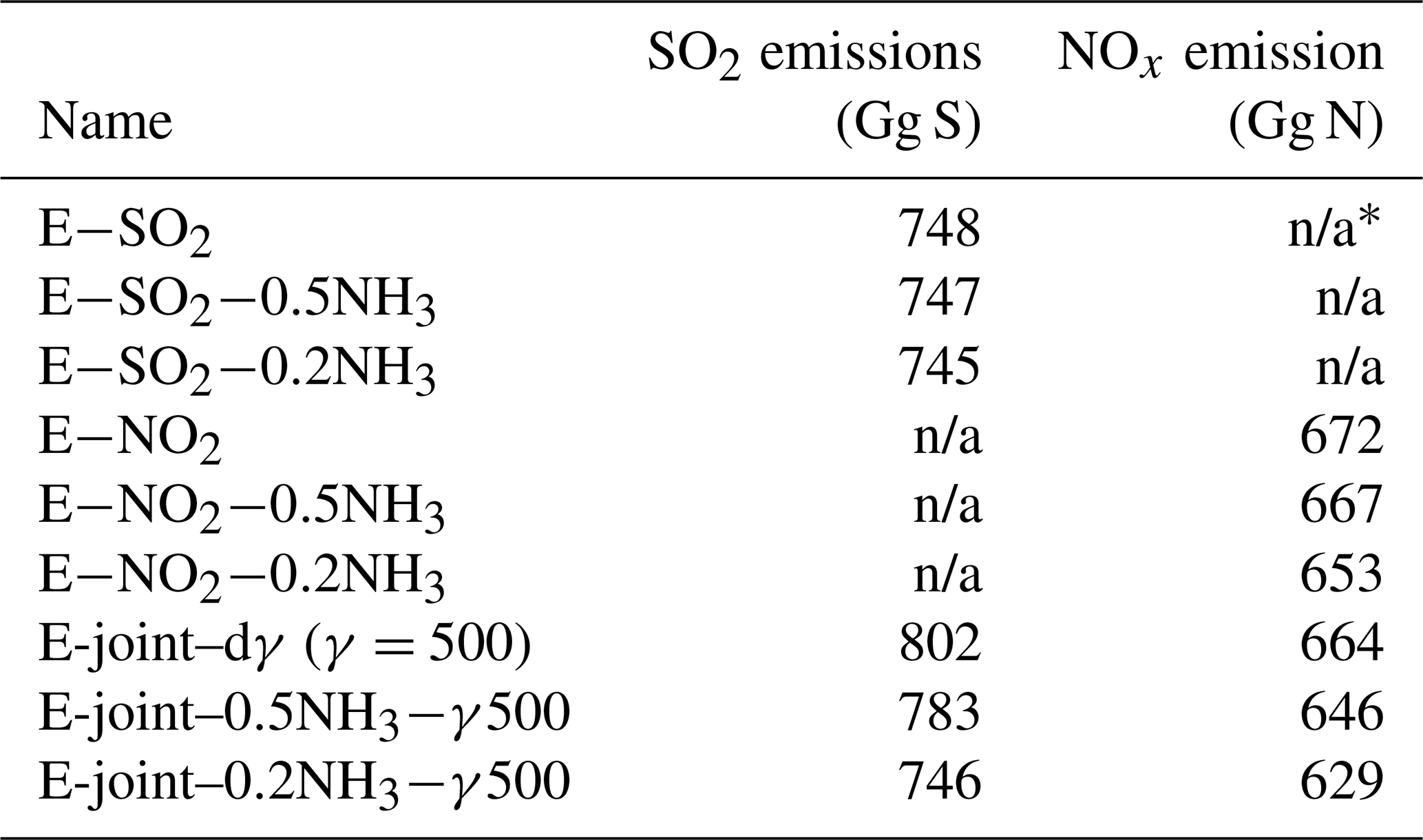
Table 1 Different experimental design for using OMPS SO₂ and NO₂ to constrain corresponding emissions over China for October 2013.

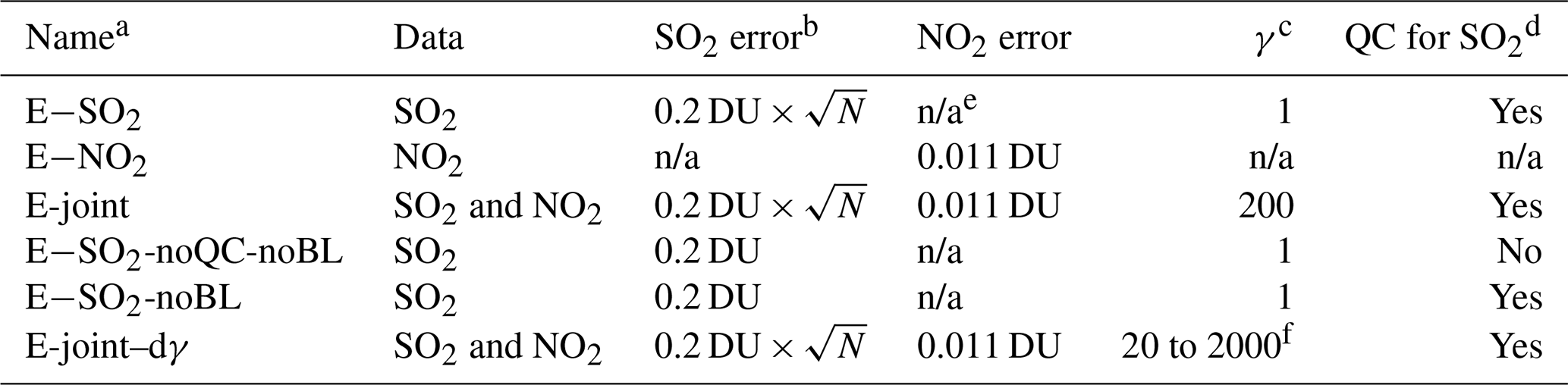
^a See description of these names in detail in Sect. 3.2. ^b N in this column is the number of OMPS overpasses that have SO₂ observations in the 2×2.5 GEOS-Chem grid cell. ^c γ is a parameter used to balance SO₂ and NO₂ observation terms in the cost function. ^d OMPS SO₂ retrievals in the 2×2.5 grid cell where the prior GEOS-Chem simulation is less than 0.1 DU are removed. ^e n/a stands for not applicable. ^f All of the following γ values are used: 20, 50, 100, 300, 500, 1000, 1500, and 2000.

3.2.1 Control experiments

The first control experiment is E−SO₂ (Table 1), in which only OMPS SO₂ tropospheric VCDs are used to constrain SO₂ emissions by removing the second additive term on the right side of Eq. (1). Consequently, γ is set to unity. If the OMPS SO₂ tropospheric VCD error is set to 0.2 DU (Yang et al., 2013) for every pixel, the SO₂ observational term in the cost function (first term on the right side of Eq. 1) over the North China Plain is much larger than that over southwestern China (Fig. 2b), which yields a high possibility of overconstraining the former and underconstraining the latter. The spatially unbalanced cost function is caused by cloud screening, as the number of observations over southwestern China is much lower than that over the North China Plain (Fig. 2a). To balance the cost function by accounting for this difference in the number of observations, the SO₂ observation error is set to 0.2 DU multiplied by the square root of the number of OMPS overpasses that have SO₂ observation in the $\mathrm{2}{}^{\circ }\times \mathrm{2.5}{}^{\circ }$ GEOS-Chem grid cell. The balance approach essentially normalizes observation terms in the cost function by the observation counts, which has been used in our study (Xu et al., 2015) to optimally invert aerosol optical properties from the skylight polarization and intensity measurements by the AErosol RObotic NETwork (AERONET).

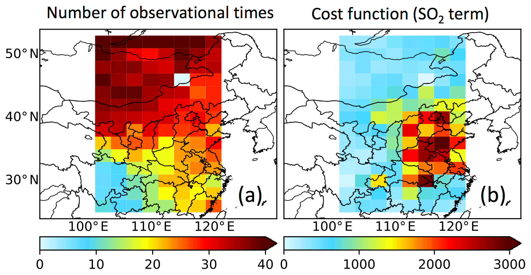
Figure 2 Panels (a) and (b) show the numbers of the OMPS overpass time that provides SO₂ VCD retrievals and the SO₂ term in the cost function at the first iteration, respectively, in October 2013.

In the second experiment, E−NO₂, OMPS NO₂ tropospheric VCDs alone are used to constrain NO_x emissions by removing the first additive term on the right side of Eq. (1). Due to cloud screening, much more OMPS NO₂ observations exist over the North China Plain than over southwestern China, which also could lead to a spatially unbalanced cost function if the OMPS NO₂ observation error is uniform. The OMPS NO₂ observation error is, however, assumed to be 0.011 DU (Yang et al., 2014) for every pixel in this study, regardless of location, because the NO_x emissions adjustments during the inverse modeling process are supposed to be mainly over the North China Plain where prior NO_x emissions are much larger than those over southwestern China. In this study, we optimize emission scale factors rather than the emissions themselves. As a result, emissions are adjusted mainly at locations where prior emissions are large and kept as zero for those ($\mathrm{2}{}^{\circ }\times \mathrm{2.5}{}^{\circ }$) grid boxes of zero prior emissions.

In the third experiment, E-joint, both the SO₂ and NO₂ from OMPS are used simultaneously for two reasons. Firstly, SO₂ and NO₂ concentrations can affect each other through several pathways. For example, Qu et al. (2019b) showed that the change in SO₂ or NO_x emissions leads to the changes in O₃ and OH concentrations and hence the changes in SO₂ and NO₂ oxidations. Here, we will explore how the optimization results may depend on the uncertainty of ammonia emissions (as elaborated in Sect. 3.2.2). Secondly, the computational time is reduced by ∼ 50 % in the joint assimilation as compared to separate assimilations when computational resources are restricted to running individual inversions sequentially (as opposed to in parallel), and energy usage is also saved; the latter requires the realization of GEOS-Chem adjoint twice, while only once is needed by the former.

In the E-joint experiment, observational terms for SO₂ and NO₂ in the cost function should be balanced through setting γ in Eq. (1). When it is not balanced, SO₂ observations have very little impact on the inversion results as the optimization algorithm will firstly minimize the observational term for NO₂ unless many more iterations than is computationally feasible are performed, which is caused by the fact that the observational error and valid number of NO₂ observations are respectively smaller and larger than the counterparts of SO₂. We thus subjectively derive γ in a nonarbitrary way in order to focus equally on both species, thereby tackling the imbalance in their observational constraints. In this manner, the cost function is defined to serve the purpose of joint inversion of SO₂ and NO₂ emissions. Initially, we set γ to be the ratio of the number of NO₂ observations to the number of SO₂ observations. This approach is not feasible here as the SO₂ observational error in E−SO₂ is much larger than the NO₂ observational error in E−NO₂; not only does the number of observations play a role, but the observation error also has important impacts on balancing the cost function. If γ is simply set as unity, the NO₂ observational term in Eq. (1) is a factor of ∼ 200 larger than the SO₂ observational term, which can lead to OMPS SO₂ in the E-joint experiment being negligible. Consequently, to balance the two terms, γ is set as 200 (ratio of observational term in E−NO₂ to that in E−SO₂) in E-joint, and sensitivity experiments using different values of γ are conducted (see Sect. 3.2.2). A similar balance approach that adjusts the contribution of observation terms in the cost function has been used in previous work that assimilates satellite trace gas retrievals to invert emissions (Qu et al., 2019b) or invert the aerosol optical properties from skylight polarization measurements of AERONET (Xu et al., 2015).

3.2.2 Sensitivity experiments

To investigate the impacts of data quality control and spatially balancing the cost function on optimizing SO₂ emissions only, we design two sensitivity experiments. The first is E−SO₂-noQC-noBL, which is similar to E−SO₂ except that (1) OMPS SO₂ retrievals in the $\mathrm{2}{}^{\circ }\times \mathrm{2.5}{}^{\circ }$ grid cell where the prior GEOS-Chem simulation is less than 0.1 DU are also assimilated, i.e., without QC; and (2) OMPS SO₂ observation error is set as 0.2 DU for every pixel, which means we do not spatially balance the cost function. The second sensitivity experiment is E−SO₂-noBL, in which the cost function is not spatially balanced, and it uses the same setting as E−SO₂ except for assuming an observation error of 0.2 DU uniformly.

To evaluate the effect of γ (of 200) in E-joint, we further test γ values of 20, 50, 100, 300, 500, 1000, 1500, and 2000 in the joint inversions; hereafter these experiments are named E-joint–dγ. Through these sensitivity experiments, we study the proper γ range for jointly assimilating OMPS SO₂ and NO₂. In future studies that may be conducted to jointly assimilate OMPS SO₂ and NO₂ for other months to obtain a long-term optimized emission inventory, setting proper γ values for each month based on the range with easy adjustment according to the numbers of OMPS SO₂ and NO₂ observations and their associated errors is proposed.

NH₃ emissions are not optimized in our inverse modeling and yet their uncertainty is up to 153 % over China (Kurokawa et al., 2013). Thus, it is important to evaluate how this uncertainty may affect posterior SO₂ and NO_x emissions. Wang et al. (2013) emphasized the importance of controlling NH₃ to alleviate PM_2.5 pollution over China; however, it could worsen acid rain (Liu et al., 2019). Changes in NH₃ emissions are expected to change ammonium and nitrate aerosol concentrations, or the aerosol surface area for heterogeneous N₂O₅ chemistry, hence affecting NO₂ concentrations or posterior NO_x emissions in the inverse modeling. The change in posterior NO_x emissions is expected to lead to the change in posterior SO₂ emissions in the joint inverse modeling. Thus, we shall investigate how the optimized SO₂ and NO₂ emission inventories would change if NH₃ emissions were reduced to 50 % and 20 %. Correspondingly, all these experiments are summarized in Table 2. $\mathrm{E}-{\mathrm{SO}}_{\mathrm{2}}-\mathrm{0.5}{\mathrm{NH}}_{\mathrm{3}}$, $\mathrm{E}-{\mathrm{NO}}_{\mathrm{2}}-\mathrm{0.5}{\mathrm{NH}}_{\mathrm{3}}$, and E-joint–0.5NH₃−γ500 in Table 2 are similar to E−SO₂, E−NO₂, and E-joint–dγ (γ=500) in Table 1, respectively, but NH₃ emissions are set to 50 % of the original values. Similarly, $\mathrm{E}-{\mathrm{SO}}_{\mathrm{2}}-\mathrm{0.2}{\mathrm{NH}}_{\mathrm{3}}$, $\mathrm{E}-{\mathrm{NO}}_{\mathrm{2}}-\mathrm{0.2}{\mathrm{NH}}_{\mathrm{3}}$, and E-joint–0.2NH₃−γ500 are the scenarios in which NH₃ emissions are set to 20 % of the original values.

Table 2 Different experimental design for assessing the impacts of NH₃ emission inventories on using OMPS SO₂ and NO₂ to constrain corresponding emissions over China for October 2013^a.

^a Data quality control and observation errors are the same as E-joint in Table 1. ^b See description of these names in detail in Sect. 3.2. ^c γ is a parameter used to balance SO₂ and NO₂ observation terms in the cost function. ^d n/a stands for not applicable.

Figure 3 Comparisons of VCDs of SO₂ and NO₂ from the OMPS and the GEOS-Chem prior and posterior simulations in October 2013 over China. The first row is SO₂ VCDs from the OMPS (a), the prior simulation (b), the E−SO₂ posterior simulation (c), and the E-joint posterior simulation (d). The second row is NO₂ tropospheric VCDs from the OMPS (e), the prior simulation (f), the E−NO₂ posterior simulation (g), and the E-joint posterior simulation (h). The third row is the SO₂ VCD scatter plots of the GEOS-Chem prior (i), the E−SO₂ posterior (j), and the E-joint posterior (k) versus the OMPS, respectively. The last row is the NO₂ tropospheric VCD scatter plots of the GEOS-Chem prior (l), the E−NO₂ posterior (m), and the E-joint posterior (n) versus the OMPS, respectively. The linear correlation coefficient (R), linear regression equation, root mean squared error (RMSE), normalized mean bias (NMB), mean bias (MB), and number of observations (N) are shown over scatter plots.

3.3 Evaluation statistics

We use the linear correlation coefficient (R), root mean square error (RMSE), mean bias (MB), normalized mean bias (NMB), normalized standard deviation (NSD), and normalized centered root mean square error (NCRMSE) as measures to evaluate GEOS-Chem SO₂ and NO₂ VCD simulations with satellite (OMPS and OMI) observations. NSD is the ratio of the standard deviation of the simulation to the standard deviation of the observation. NCRMSE is similar to RMSE, but the impact of bias is removed. This is shown in Eq. (2), where i is the ith grid cell, N is the total number of grid cells, M_i and O_i are the ith GEOS-Chem simulation and satellite observation, respectively, and $\stackrel{\mathrm{‾}}{M}$ and $\stackrel{\mathrm{‾}}{O}$ are averages of GEOS-Chem simulation and satellite observation, respectively. A composite summary of these statistics is provided by the Taylor diagram (Taylor, 2001), which is a quadrant that summarizes R (shown as cosine of polar angle), NSD (shown as radius from the quadrant center), and NCRMSE (shown as radius from the observation which is located at the point where R and NSD are unity).

$$\begin{array}{}\text{(2)}& \mathrm{NCRMSE}={\displaystyle \frac{\sqrt{\frac{\mathrm{1}}{N}{\sum }_{i=\mathrm{1}}^N[\left(M_i-\stackrel{\mathrm{‾}}{M}\right)-(O_i-\stackrel{\mathrm{‾}}{O}){]}^{\mathrm{2}}}}{\sqrt{\frac{\mathrm{1}}{N}{\sum }_{i=\mathrm{1}}^N(O_i-\stackrel{\mathrm{‾}}{O}{)}^{\mathrm{2}}}}}\end{array}$$

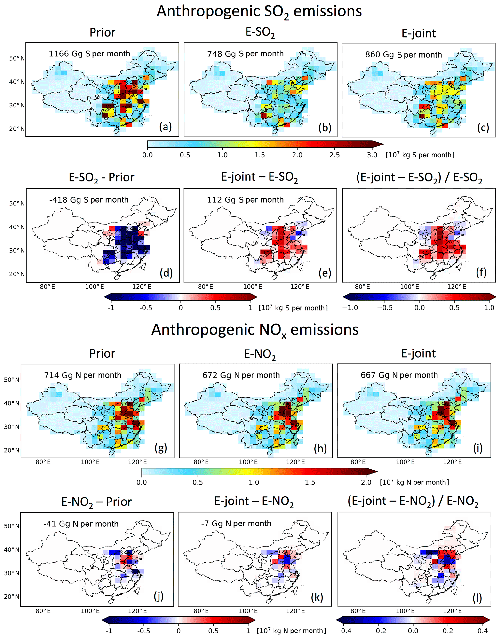
Figure 4 The top is anthropogenic SO₂ emissions from prior MIX 2010 (a), posterior E−SO₂ (b), posterior E-joint (c), the difference between posterior E−SO₂ and prior MIX 2010 (d), the difference between posterior E-joint and posterior E−SO₂ (e), and the relative difference between posterior E-joint and posterior E−SO₂ (f) for October 2013. The bottom is similar to the top except that (1) it is for NO_x and (2) E−SO₂ is replaced by E−NO₂.

4 Results

4.1 Separate and joint assimilations of SO₂ and NO₂

4.1.1 Self-consistency check

The cost functions are reduced by 41.6 %, 27.6 %, and 28.6 % for E−SO₂, E−NO₂, and E-joint, respectively, and the results are shown in Fig. 3. Noticeably, hot spots of SO₂ VCDs over the North China Plain and the Sichuan Basin are shown in the OMPS observations (Fig. 3a), prior (Fig. 3b), posterior E−SO₂ (Fig. 3c), and posterior E-joint (Fig. 3d) simulations; however, the prior simulation has an NMB of 106.5 % (Fig. 3i) when compared with OMPS. The SO₂ NMB (106.5 %) between GOES-Chem prior simulation and OMPS is much larger than the NMB (−6.8 %, Fig. S1) caused by the difference in SO₂ vertical profiles between the OMPS SO₂ retrieval algorithm and current prior simulation; thus the averaging kernel is not considered in the OMPS SO₂ observation operator. This large positive NMB decreases to 13.0 % and 38.3 % in the posterior E−SO₂ (Fig. 3j) and E-joint (Fig. 3k) simulations with an RMSE decreasing from 0.42 to 0.13 and 0.20 DU and R increasing from 0.62 to 0.72 and 0.64, respectively. Large NO₂ values are found over the North China Plain and eastern China with large NO_x emissions from the transportation sector (Fig. 3e–h). Comparing with OMPS NO₂, GEOS-Chem results have an RMSE of 0.05 DU in the prior simulation (Fig. 3l) and reduce to 0.02 and 0.03 DU for E−NO₂ (Fig. 3m) and E-joint (Fig. 3n), with R increasing from 0.95 to 0.99 and 0.98, respectively.

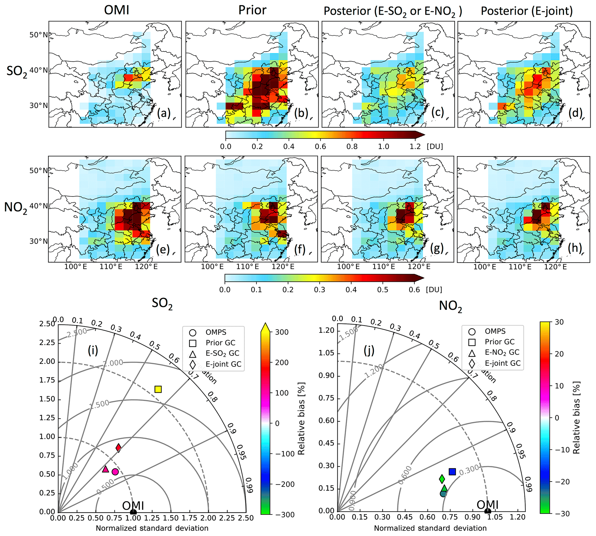
Figure 5 Comparisons of VCDs of SO₂ and NO₂ from the OMPS and the GEOS-Chem prior and posterior simulations with that from the OMI in October 2013 over China. The first row is SO₂ VCDs from the OMI (a), the prior simulation (b), the E−SO₂ posterior simulation (c), and the E-joint posterior simulation (d). The second row is NO₂ tropospheric VCDs from the OMI (e), the prior simulation (f), the E−NO₂ posterior simulation (g), and the E-joint posterior simulation (h). The third row is Taylor diagrams for comparing GEOS-Chem simulations (squares for prior, triangles for posterior E−SO₂ or E−NO₂, and diamonds for E-joint) and OMPS observations (circles) with OMI SO₂ (i) and NO₂ (j).

Similarly, the averaging kernel is not considered in the OMPS NO₂ observation operator for optimization for the following reasons. First, the OMPS NO₂ retrieval differences due to the profile differences can lead to a NMB of −7.5 % (Fig. S2), which is still smaller than the prior GEOS-Chem simulation NMB (10.9 %, Fig. 3l). Second, a NMB of 10.9 % for the model NO₂ VCD simulation is not a very large value, as the difference between satellite NO₂ VCD retrievals and ground-based measurements could be comparable to this value. For example, Krotkov et al. (2017) show that OMI NO₂ VCD retrievals, on average, are ∼ 10 % larger than the ground-based Fourier-transform infrared (FTIR) spectrometer. Thus, current research should mainly focus on the change in the spatial distribution (such as linear correlation coefficient) rather than the bias of the prior and posterior GEOS-Chem NO₂ VCD simulation. Finally, given that the linear correlation coefficient between OMPS retrievals and those that are modified through integration of the averaging kernel and NO₂ vertical profile from this study is as large as 0.99, the averaging kernel is not dealt with in the development of the OMPS NO₂ observation operator. In general, the E−SO₂ and E−NO₂ posterior simulations show better results than E-joint, which may be affected by the value of γ, which we will discuss in Sect. 4.3.

4.1.2 Emissions

The anthropogenic SO₂ and NO_x prior MIX emissions for October 2010 and posterior emissions from E−SO₂, E−NO₂, and E-joint for October 2013 are shown in Fig. 4. SO₂ and NO_x hot spots are found in the prior emissions over both the North China Plain and eastern China, while large SO₂ emissions are also found in southwestern China. Anthropogenic SO₂ emissions over China are 1166 Gg S in prior MIX for October 2010 (Fig. 4a), dropping 418 Gg S (Fig. 4b) and 306 Gg S (Fig. 4c), or 35.8 % and 26.2 %, in E−SO₂ and E-joint, respectively, for October 2013. The differences between the estimates of this study and the MIX emission inventory, however, should not be considered as trends, and they are derived from different approaches. Posterior E-joint total anthropogenic SO₂ emissions are 112 Gg, or 15 % larger than E−SO₂, over China (Fig. 4e). Regionally, positive differences between E-joint and E−SO₂ anthropogenic SO₂ emissions are found over most areas of central China and eastern China, and a relative difference of up to 100 % is found over Shanxi Province (Fig. 4f). Grids with large differences are generally in locations where prior anthropogenic SO₂ emissions are larger, which means the pattern is affected by the fact that the algorithm optimizes emission scale factors rather than emissions directly. Anthropogenic NO_x emissions over China are reduced by 5.8 % and 6.5 %, from 714 Gg N in prior MIX for October 2010 (Fig. 4g) to 672 Gg N (Fig. 4h) in E−NO₂ and 667 Gg N (Fig. 4i) in E-joint for October 2013. Although the relative difference between E-joint and E−NO₂ proved to be less than 2 % in terms of total anthropogenic NO_x emissions over China (Fig. 4k), it is up to 40 % over Shanxi Province, and both grids with large positive differences and grids with large negative differences exist over the North China Plain (Fig. 4l).

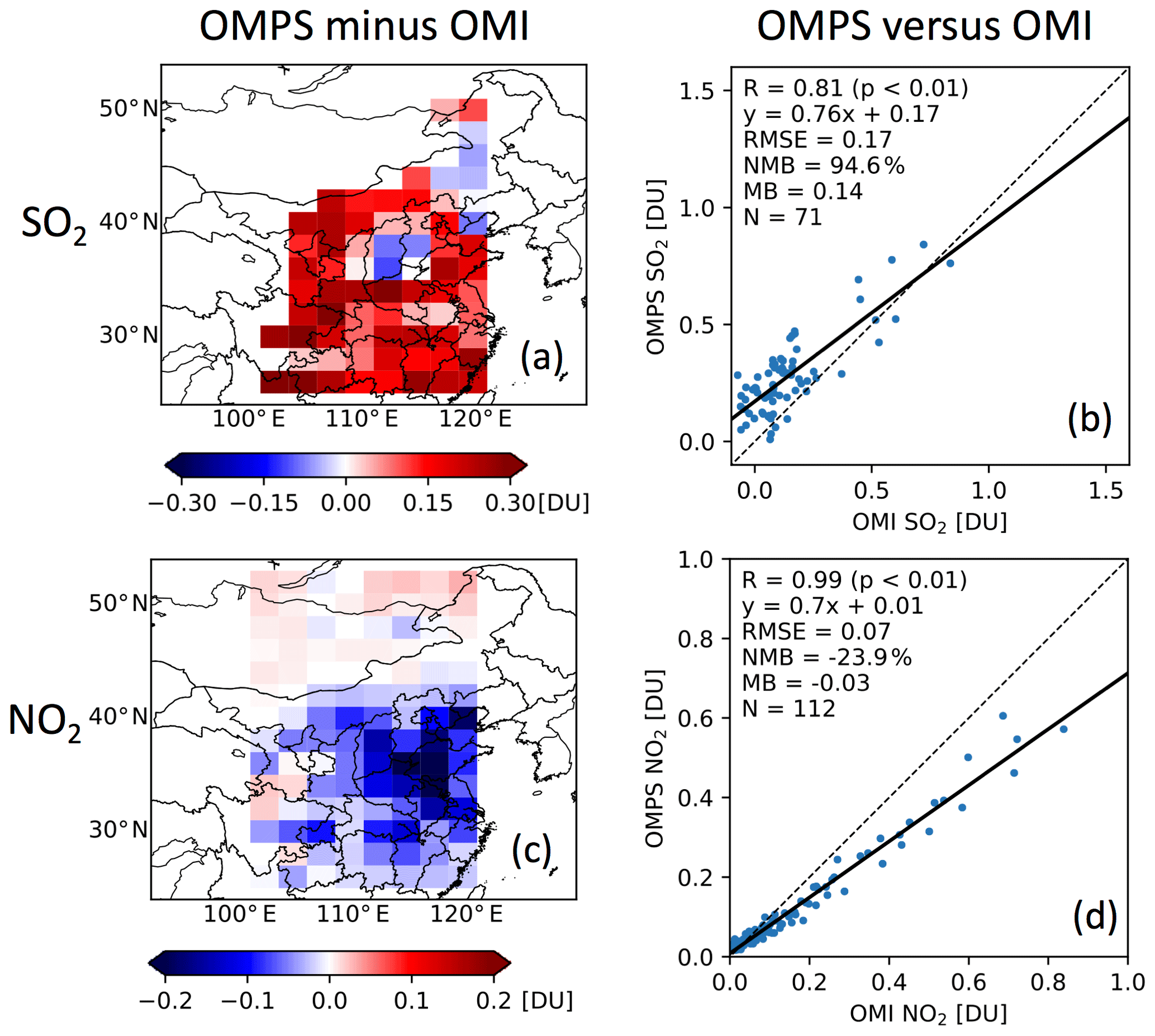
Figure 6 Panels (a) and (b) show the difference between OMPS and OMI SO₂ and the scatter plot of OMPS versus OMI SO₂. Panels (c) and (d) are similar to (a) and (b) but for NO₂. The linear correlation coefficient (R), linear regression equation, root mean squared error (RMSE), normalized mean bias (NMB), mean bias (MB), and number of observations (N) are shown over scatter plots.

4.1.3 Independent evaluation with OMI data

The optimized emission inventories are evaluated by comparing prior and posterior GEOS-Chem simulations of SO₂ and NO₂ with OMI VCDs as shown in Fig. 5. We only focus on regions covered by OMPS observations, although smaller changes in emissions exist in outskirt regions where OMPS observations are not used. High SO₂ levels are shown over the North China Plain and the Sichuan Basin in both the prior and posterior simulations, while OMI only observes hot spots over the former region (Fig. 5a–d). When validating with OMI SO₂ VCDs, the NMB is ∼ 300 % in the prior simulation, and it reduces to ∼ 100 % in E−SO₂ and ∼ 130 % in E-joint (Fig. 5i). Not only is the NMB reduced, but the spatial distributions are also improved, with the NCRMSE reducing from ∼ 1.6 in the prior simulation to ∼ 0.7 in E−SO₂ and ∼ 0.8 in E-joint, which is much closer to ∼ 0.6 when comparing OMPS observations with OMI observations (Fig. 5i). For NO₂, OMI observations and the prior and posterior simulations show large NO₂ concentrations over the North China Plain and eastern China (Fig. 5e–h). The improvements for E−NO₂ and E-joint are reflected in terms of R when evaluating with OMI tropospheric VCDs, although the two experiments show a larger negative NMB than the prior simulation (Fig. 5j). In all the evaluations, OMI SO₂ and NO₂ VCD retrievals are not corrected by calculating new air mass factors that are derived from integrating scattering weights and corresponding vertical profiles of GEOS-Chem simulations of this study. However, Fig. S4 shows similar improvements if new air mass factors are applied, although statistic metric values are slightly different.

Here, OMPS observations and GEOS-Chem simulations are compared with OMI observations as an evaluation of posterior emission inventories, but it is not assumed that OMI provides the true status of SO₂ and NO₂ in the atmosphere. OMI and OMPS observe the same trend direction of SO₂ (NO₂) over China, but the strengths of the trend are quite different (Wang and Wang, 2020). The OMPS SO₂ average is ∼ 0.14 DU, or ∼ 95 % larger than OMI SO₂, and the R of the two products is 0.81 (Fig. 6b). Thus, it is reasonable that posterior SO₂ is larger than OMI observations by ∼ 100 % in E−SO₂ and ∼ 130 % in E-joint. OMPS NO₂ is ∼ 24 % smaller than OMI (Fig. 6d), which explains why the posterior NO₂ simulations have a larger negative NMB than the prior simulation when compared with the OMI observations. Our analysis also shows that the systematic difference among various satellite products for the same species (such as SO₂ or NO₂) can lead to biases in constraining emissions, but the posterior GEOS-Chem simulations still show better results in terms of the spatial distribution of SO₂ and NO₂.

Figure 7 SO₂ VCD in October 2013 from OMPS (a), prior GEOS-Chem simulation (b), posterior GEOS-Chem simulation through the use of all OMPS data in the red box (c), and posterior GEOS-Chem simulation through the use of only OMPS data that are in the grid cell where GEOS-Chem prior simulation of VCD is larger than 0.1 DU. For posterior simulation, we only plot SO₂ VCD over grid cells where OMPS data are used to constrain emissions. M and S point to a grid cell in Inner Mongolia and the Sichuan Basin, respectively.

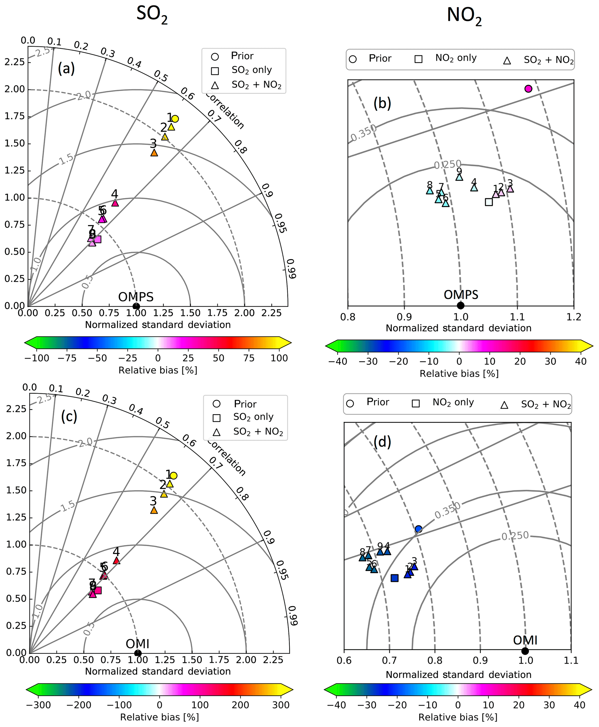
Figure 8 Taylor diagram comparing GEOS-Chem simulation with OMPS (a for SO₂ and b for NO₂) or OMI (c for SO₂ and d for NO₂) in October 2013. Circles, squares, and triangles represent GEOS-Chem simulations using prior MIX 2010 emissions, posterior emissions constrained by single species (E−SO₂ for a and c, E−NO₂ for b and d), and posterior emissions constrained through joint inversion (E-joint), respectively. Different triangles labeled by numbers represent different γ values in Eq. (1), and 1 through 9 correspond to 20, 50, 100, 200, 300, 500, 1000, 1500, and 2000, respectively.

4.2 The impacts of QC and spatial balance

The results of E−SO₂-noQC-noBL and E−SO₂-noBL are compared with E−SO₂ to show the impacts of QC and spatial balance. Both OMPS retrievals and the GEOS-Chem prior simulations show that SO₂ VCDs over Inner Mongolia and the Sichuan Basin (grid cells M and S, respectively in Fig. 7) are smaller than those over the North China Plain; this pattern reverses in the posterior E−SO₂-noQC-noBL simulation where SO₂ over the North China Plain becomes smaller than that over grid cells M and S. Grid cell M becomes more reasonable after conducting the data quality control by removing OMPS SO₂ in any grid cells where prior GEOS-Chem SO₂ VCDs are less than 0.1 DU (e.g., as in E−SO₂-noBL, as shown in Fig. 7d). QC helps to improve models over grid cell M, as the data removed are close to Inner Mongolia and are generally less than 0.1 DU, which is comparable to the retrieval error. SO₂ over grid cell S from E−SO₂-noBL (Fig. 7d) is, however, still larger than that over the North China Plain, compared with the better spatial pattern from E−SO₂ (Fig. 3c). Thus, QC and spatial balancing of the cost function together improve the spatial pattern of the posterior GEOS-Chem SO₂ VCD simulation.

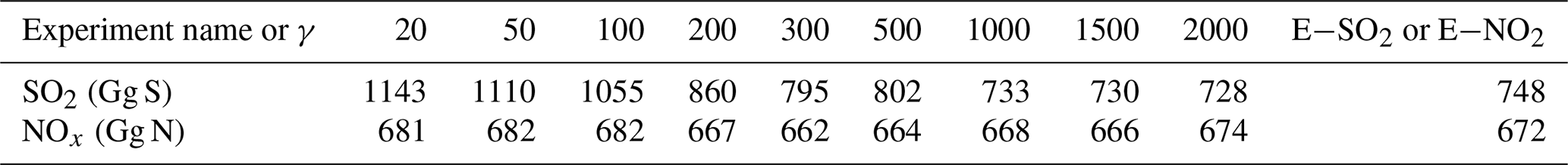
Table 3 Posterior anthropogenic emissions for October 2013 from E-joint, E-joint–dγ, E−SO₂, and E−NO₂.

4.3 The impacts of γ on joint assimilations

In addition to setting γ as 200 in E-joint, we test the impacts of using various γ values on joint assimilation in E-joint–dγ for October 2013. All the SO₂ and NO₂ VCDs from prior and posterior E-joint and E-joint–dγ simulations are compared with OMPS counterparts (Fig. 8a, b). Regardless of the γ values used, all the posterior simulations of SO₂ show smaller NMB and NCRMSE than the prior simulation when validating against OMPS counterparts, but the extents of improvement vary. When γ is 20, 50, or 100, the SO₂ terms are obviously underconstrained, and GEOS-Chem SO₂ NCRMSE, evaluated with OMPS observations, changes from ∼ 1.8 in the prior simulation to in the range of ∼ 1.4 to ∼ 1.7 in the posterior E-joint–dγ simulations, which are much larger than ∼ 0.7 in E−SO₂ (Fig. 8a). Similarly, when γ is no larger than 100, the bias of GEOS-Chem SO₂, validated with OMPS observations, only reduces from ∼ 100 % to ∼ 75 %, compared to ∼ 25 % in E−SO₂ (Fig. 8a), and the posterior SO₂ emissions are in the range of 1055 to 1143 Gg S, which is much larger than 748 Gg S from E−SO₂ (Table 3). When γ is in the range of 200 to 2000, the SO₂ simulation results and emissions from joint assimilations are more similar to those from E−SO₂ than those with γ no larger than 100 (Fig. 8a and Table 3). Similar to SO₂, the GEOS-Chem simulations of NO₂ in the sensitivity experiments improve in terms of R and NCRMSE in all joint assimilation tests, but the significance of γ is less than that for SO₂. NO₂ NCRMSE is ∼ 0.4 in the prior simulation when evaluating with OMPS counterparts, compared to the range of ∼ 0.2 to ∼ 0.25 in E-joint, E-joint–dγ, and E−NO₂ (Fig. 8b). The posterior NO_x emissions are in the range of 662 to 682 Gg N, compared with 672 Gg N in E−NO₂ (Table 3).

The impacts of γ are also reflected when evaluating SO₂ and NO₂ simulations with OMI retrievals (Fig. 8c, d). Small γ values of 20, 50, and 100 lead to a much larger bias and NCRMSE for SO₂ from E-joint–dγ than that from E−SO₂. For NO₂, these small γ values make results from E-joint–dγ very similar to that from E−NO₂.

Considering all of the above analyses, the results with γ in the range of 200 to 2000 are deemed acceptable. The E-joint–dγ ($\mathrm{200}\le \mathit{\gamma }\le \mathrm{2000}$) emissions are within −3 % to 15 % of E−SO₂ for SO₂ and ±2 % of E−NO₂ for NO_x in terms of total anthropogenic SO₂ and NO_x emissions over China. When evaluating with OMPS observations, the NCRMSE values using the posterior emissions from the separate and joint ($\mathrm{200}\le \mathit{\gamma }\le \mathrm{2000}$) inversions are ∼ 60 % and ∼ 45 %–60 % smaller than those using the prior emissions for SO₂, respectively, and ∼ 50 % and ∼ 38 %–50 % smaller than those using the prior emissions for NO₂, respectively.

Table 4 Posterior anthropogenic emissions for October 2013 under different NH₃ emission scenarios.

^* n/a stands for not applicable.

Figure 9 Relative changes in posterior SO₂ (a–d) and NO_x (e–h) emissions from the scenarios of perturbing NH₃ emissions with respect to that using the original NH₃ emission inventory. Panels (a) and (b) show relative changes in posterior SO₂ emissions from $\mathrm{E}-{\mathrm{SO}}_{\mathrm{2}}-\mathrm{0.5}{\mathrm{NH}}_{\mathrm{3}}$ and $\mathrm{E}-{\mathrm{SO}}_{\mathrm{2}}-\mathrm{0.2}{\mathrm{NH}}_{\mathrm{3}}$ with respect to that from E−SO₂, respectively. Panels (c) and (d) show relative changes in posterior SO₂ emissions from E-joint–0.5NH₃-γ500 and E-joint–0.2NH₃−γ500 with respect to that from E-joint–dγ (γ=500), respectively. Panels (e) and (f) show relative changes in posterior NO_x emissions from $\mathrm{E}-{\mathrm{NO}}_{\mathrm{2}}-\mathrm{0.5}{\mathrm{NH}}_{\mathrm{3}}$ and $\mathrm{E}-{\mathrm{NO}}_{\mathrm{2}}-\mathrm{0.2}{\mathrm{NH}}_{\mathrm{3}}$ with respect to that from E−NO₂, respectively. Panels (g) and (h) are similar to (c) and (d), respectively, but for posterior NO_x emissions. Minimum and maximum are shown in brackets.

When evaluating with OMI retrievals, joint inversion shows better results than separate inversion for SO₂ or NO₂, but not both, depending on the value of γ . When γ is 20, 50, or 100, the NO₂ NCRMSE for E-joint–dγ appears to be smaller than that for E−NO₂, but the SO₂ NCRMSE for E-joint–dγ is larger than that for E−SO₂. Conversely, when γ is 1000, 1500, or 2000, the SO₂ NCRMSE for E-joint–dγ is smaller than that for E−SO₂, but the NO₂ NCRMSE for E-joint–dγ is larger than that for E−NO₂. This is similar to the findings by Qu et al. (2019b) in which the months when the joint inversion shows better results than the separate inversion for SO₂ (NO₂) have a worse result for NO₂ (SO₂). The benefit of joint inversion for improving only one species is similar to Qu et al. (2019b) and is likely due to the complicated relationship between these two species through different chemical pathways. For example, O₃ and OH are key species that connect the chemistry of SO₂ and NO₂, and aerosols can affect the photolysis and heterogenous chemistry. Hence, while joint inversion to improve both species cannot be demonstrated here, it should be reviewed as the first step of simultaneously assimilating multiple species (including AOD, NH₃, and other trace gases) to optimize emissions. Until then, the system is not ready to holistically evaluate the benefits of joint assimilation to improve the model in a systematic manner. It is worth noting that Xu et al. (2013) showed the feasibility of using MODIS cloud-free radiance to optimize emissions of SO₂ and NO₂ at the same time. Future research should add the aerosol optical depth or visible reflectance (as well as tropospheric O₃ if reliable) as constraints to further evaluate the benefits of joint assimilation for improving model overall performance in a systematic matter.

4.4 The impacts of NH₃ emissions

In the single-species inversions, NH₃ emission uncertainty has weaker impacts on posterior SO₂ emissions than NO_x emissions. Posterior SO₂ emissions over China are 748 Gg S in the 100 % NH₃ emission scenario (E−SO₂), and they only slightly reduce to 747 and 745 Gg S when NH₃ emissions are 50 % ($\mathrm{E}-{\mathrm{SO}}_{\mathrm{2}}-\mathrm{0.5}{\mathrm{NH}}_{\mathrm{3}}$) and 20 % ($\mathrm{E}-{\mathrm{SO}}_{\mathrm{2}}-\mathrm{0.2}{\mathrm{NH}}_{\mathrm{3}}$) of the original values, respectively (Table 4). The largest relative changes at model-grid-cell scale are only −2.5 % (Fig. 9a) for $\mathrm{E}-{\mathrm{SO}}_{\mathrm{2}}-\mathrm{0.5}{\mathrm{NH}}_{\mathrm{3}}$ and −4.7 % (Fig. 9b) for $\mathrm{E}-{\mathrm{SO}}_{\mathrm{2}}-\mathrm{0.2}{\mathrm{NH}}_{\mathrm{3}}$. All these results can be explained by considering how changes in NH₃ can potentially impact the lifetimes of SO₂ and NO₂ and hence affect SO₂ and NO₂ VCD simulations. When the NH₃ emissions are perturbed to 50 % and 20 % of the original values, GEOS-Chem SO₂ VCDs only increase up to 3.8 % and 6.1 %, respectively, in some grid cells over the Sichuan Basin in the prior simulations, and these changes are even much smaller over the North China Plain (Fig. 10a, b), as NH₃ has no direct impacts on the life cycle of SO₂. This is understandable because in GEOS-Chem, once SO₂ is oxidized to H₂SO₄, ${\mathrm{SO}}_{\mathrm{4}}^{\mathrm{2}-}$ remains as particulate sulfate regardless of whether it is neutralized by NH₃ or not (Wang et al., 2008). Hence, the reduction of NH₃ to 50 % and 20 % overall has minimal (negligible) impact on SO₂ amount in the prior simulation and the posterior separate SO₂ emission inversion.

Although the posterior NO_x emissions in the scenarios of 50 % ($\mathrm{E}-{\mathrm{NO}}_{\mathrm{2}}-\mathrm{0.5}{\mathrm{NH}}_{\mathrm{3}}$) and 20 % ($\mathrm{E}-{\mathrm{NO}}_{\mathrm{2}}-\mathrm{0.2}{\mathrm{NH}}_{\mathrm{3}}$) NH₃ emission experiments of the original values are 5 Gg N (0.7 %) and 19 Gg N (2.8 %), respectively, smaller than those when using the original (E−NO₂) NH₃ emissions over China (Table 4), the reduction is up to −4.0 % (Fig. 9e) for $\mathrm{E}-{\mathrm{NO}}_{\mathrm{2}}-\mathrm{0.5}{\mathrm{NH}}_{\mathrm{3}}$ and −9.1 % (Fig. 9f) for $\mathrm{E}-{\mathrm{NO}}_{\mathrm{2}}-\mathrm{0.2}{\mathrm{NH}}_{\mathrm{3}}$ in individual grid cells. These decreases are understood by simultaneous reduction of nitrate by 59.5 % (Fig. 12h vs. 12g) and 80.5 % (Fig. 12i vs. 12g) and ammonium by 39.6 % (Fig. 12n vs. 12m) and 67.5 % (Fig. 12o vs. 12m), which leads to large reduction of the hydrated aerosol surface area for heterogeneous N₂O₅ chemistry at night and hence overall NO₂ lifetime (Fig. 10c, d). N₂O₅ normally forms at night by reaction between NO₂ and NO₃ and thermally decomposes back to NO₂ and NO₃ (Seinfeld and Pandis, 2016), and hence the amount of N₂O₅, NO₂, and NO₃ is in equilibrium through the reversible reaction. Since the hydrolysis of N₂O₅ to form HNO₃ mainly occurs on hydrated aerosol particles (Seinfeld and Pandis, 2016), the decrease in hydrated aerosol surface area (due to reduction of NH₃ emission) leads to less hydrolysis of N₂O₅ (an important sink for atmospheric NO_x) and subsequently more NO₂ to be in equilibrium with N₂O₅ at night. As a result, the reduction of NH₃ emissions further increases the positive bias in the prior NO₂ simulations when comparing with OMPS observations, and to compensate for such a large positive bias, nonnegligible decreases in the posterior NO_x emissions are required (Fig. 9e and f). The reduction of nitrate and ammonium aerosols can also increase sunlight reaching the troposphere and hence photolysis of O₃ and NO₂. Figure S5 separates the impacts of the increase in photolysis of O₃ and NO₂ and the decrease in heterogeneous N₂O₅ chemistry on NO₂ lifetime and shows that the former is negligible compared with the latter.

The decreases in posterior SO₂ and NO_x emissions in the joint inversions caused by the reduction of NH₃ emissions are stronger than those in the separate inversions (Table 4 and Fig. 9). Although the changes in NH₃ emissions only have slight impacts on the SO₂ separate inversions (E−SO₂, $\mathrm{E}-{\mathrm{SO}}_{\mathrm{2}}-\mathrm{0.5}{\mathrm{NH}}_{\mathrm{3}}$, and $\mathrm{E}-{\mathrm{SO}}_{\mathrm{2}}-\mathrm{0.2}{\mathrm{NH}}_{\mathrm{3}}$), the posterior SO₂ emission is 802 Gg S in E-joint–dγ (γ=500) and down to 783 Gg S (decreasing by 2.4 %) and 746 Gg S (decreasing by 7.0 %) in E-joint–0.5NH₃−γ500 and E-joint–0.2NH₃−γ500, respectively (Table 4); in some grid cells, the relative reductions are up to −9.0 % (Fig. 9c) for E-joint–0.5NH₃−γ500 and −27.7 % (Fig. 9d) for E-joint–0.2NH₃−γ500. For posterior NO_x emissions at the grid cells, the relative changes are up to −15.2 % (Fig. 9g) for E-joint–0.5NH₃−γ500 and −29.4 % (Fig. 9h) for E-joint–0.2NH₃−γ500 with respect to E-joint–dγ (γ=500).

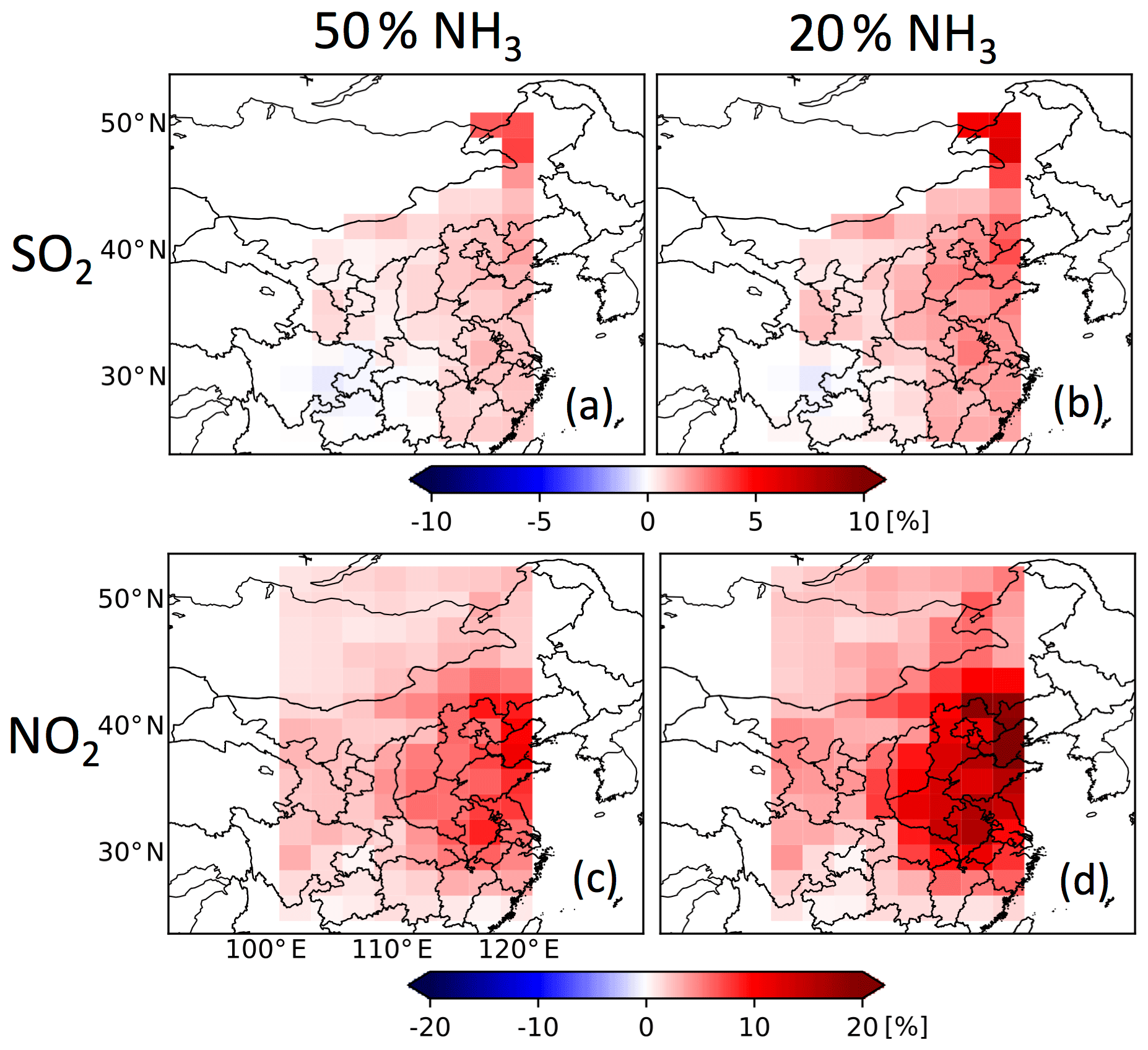
Figure 10 Relative change in GEOS-Chem SO₂ VCDs when NH₃ emissions reduce to 50 % (a) and 20 % (b), respectively, at OMPS overpassing time. Panels (c) and (d) are similar to (a) and (b), respectively, but for NO₂.

4.5 Aerosol responses to emission changes

Although SO₂ emissions over the North China Plain (E-joint–dγ (γ=500)) have decreased by more than 50 %, and NO_x emissions have also been reduced, reductions of sulfate–nitrate–ammonium (SNA) aerosol optical depth (AOD) over the same region are only up to 10 % (Fig. 11). This is because the North China Plain is mainly polluted by nitrate rather than sulfate (Fig. 12a–l), and the reduction of SO₂ emissions will increase nitrate loadings in the atmosphere (Fig. 12g–l), which is also consistent with the research of Kharol et al. (2013) that shows nitrate concentrations decrease as SO₂ emissions increase; the reduction of SO₂ emissions leads to less H₂SO₄ reacting with NH₃, which further favors the reaction of HNO₃ and NH₃ to form nitrate. As NH₃ emission changes reduce by 50 % and 80 %, ammonium column loadings decrease by ∼ 40 % and ∼ 70 % (Fig. 12g–l), respectively, and nitrate column loadings even decrease by ∼ 70 % and ∼ 90 %, respectively (Fig. 12m–r).

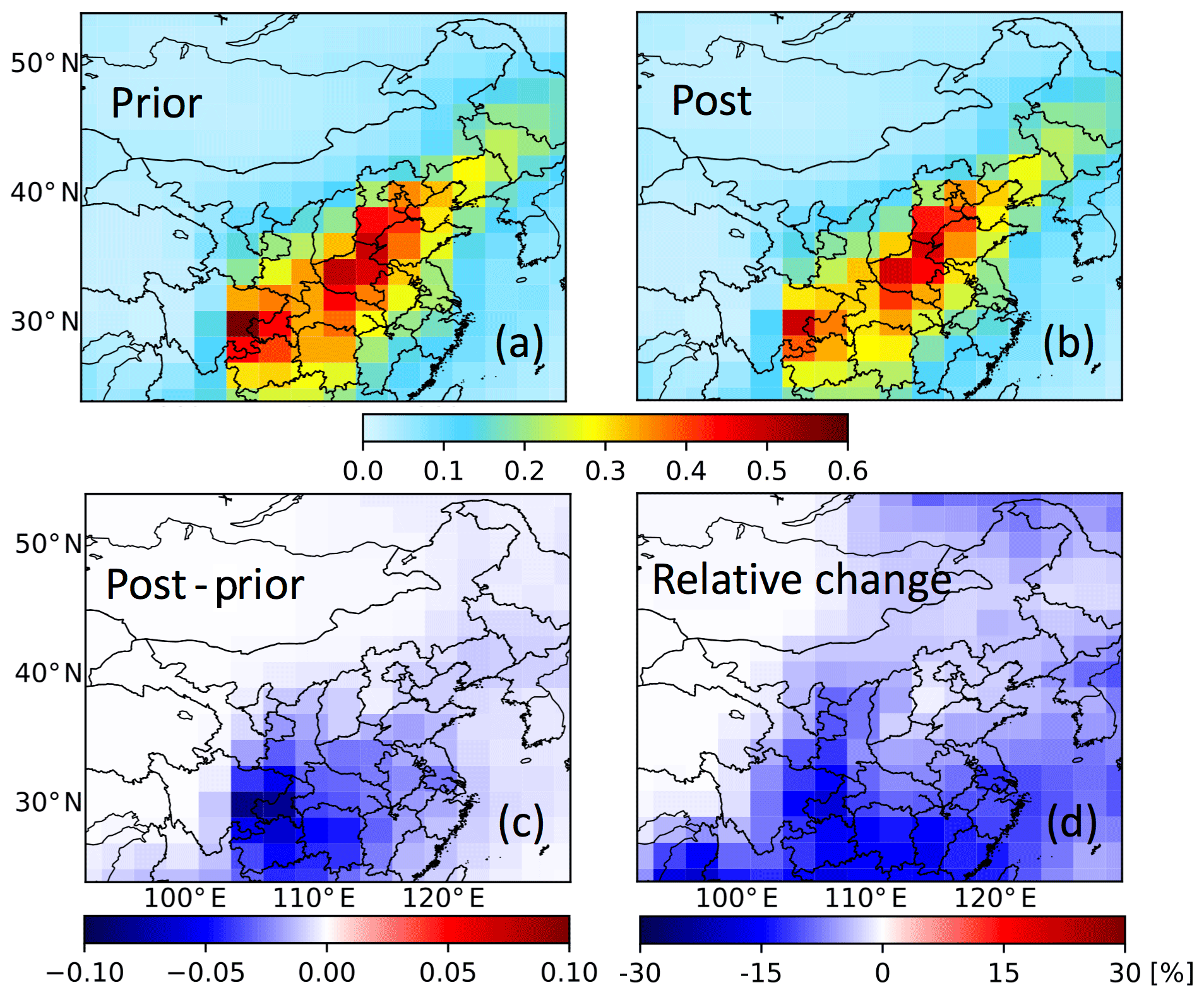
Figure 11 Sulfate–nitrate–ammonium aerosol optical depth in prior (a) and posterior joint inversion (γ=500) (b). Panel (c) shows the difference between (b) and (a), and (d) shows the relative change in percentage.

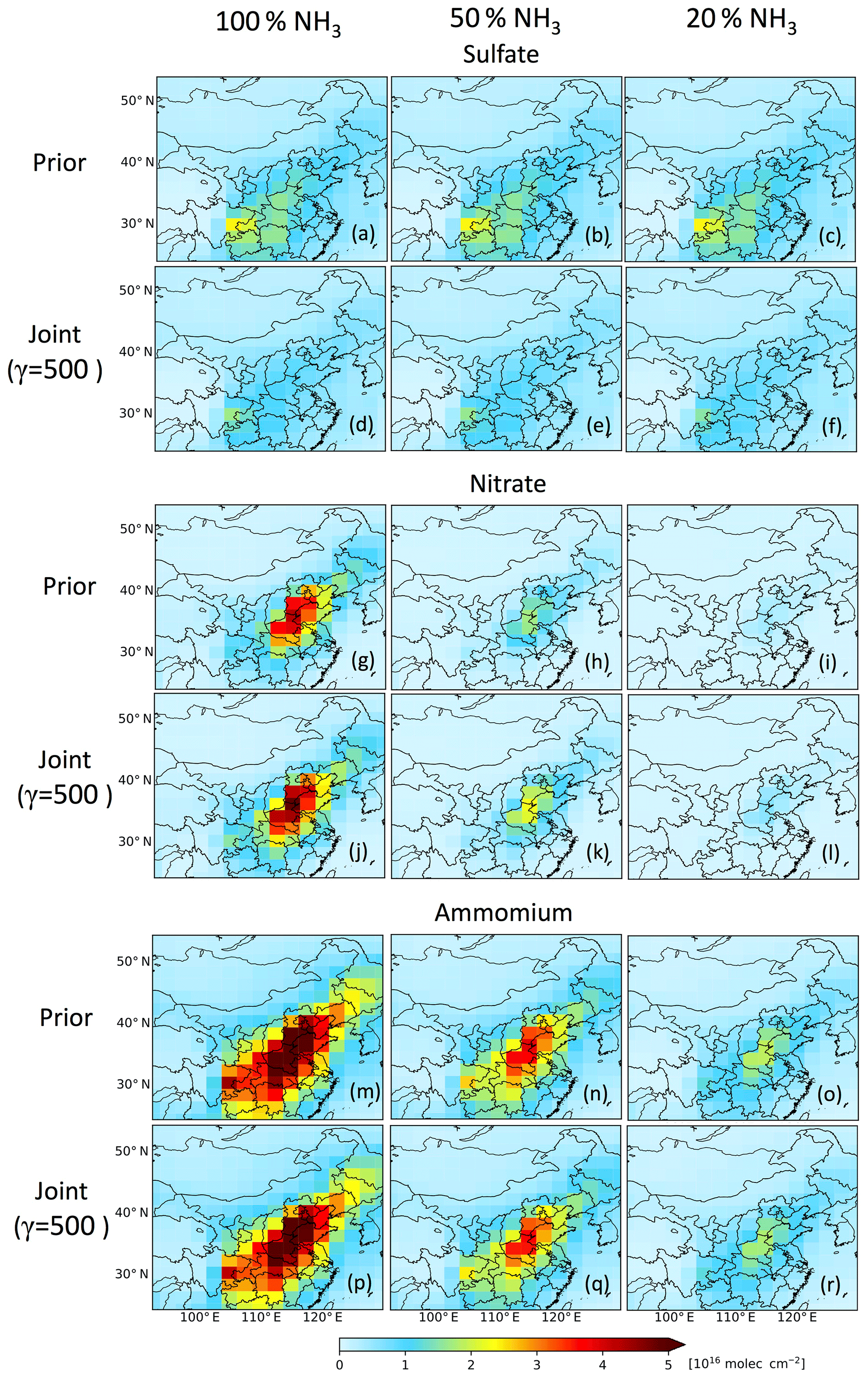
Figure 12 Sulfate, nitrate, and ammonium column loadings in different scenarios. Panels (a)–(c) show prior sulfate at 100 %, 50 %, and 20 % NH₃ emissions, respectively. Panels (d)–(f) show posterior sulfate from joint inversions (γ=500) at 100 %, 50 %, and 20 % NH₃ emissions, respectively. Panels (g–i) and (m–r) are similar to (a–f) but for nitrate and ammonium, respectively.

5 Discussion and conclusions

We developed 4D-Var observation operators for assimilating OMPS SO₂ and NO₂ VCDs to constrain SO₂ and NO_x emissions through GEOS-Chem adjoint model. The approach is applied for a case study over China for October 2013 at $\mathrm{2}{}^{\circ }\times \mathrm{2.5}{}^{\circ }$ resolution, and the MIX 2010 is used as the prior emission inventory. Several experiments of assimilating OMPS SO₂ and NO₂ separately and jointly are conducted, and SO₂ and NO₂ VCDs from the GEOS-Chem prior and posterior simulations are compared with counterparts from OMPS and OMI.

OMPS SO₂ and NO₂ retrievals are separately and jointly used to constrain their corresponding emissions. In the single-species inversions, posterior anthropogenic SO₂ and NO_x emissions are 748 Gg S and 672 Gg N for October 2013, down from 1166 Gg S and 714 Gg N in the prior MIX for October 2010, respectively. In the joint inversions of assimilating OMPS SO₂ and NO₂ simultaneously, the cost function is balanced according to the values of observational terms rather than the number of observations. When the cost function is well balanced (γ in the range of 200 to 2000), the results of the joint inversions are within −3 % to 15 % of the single-species inversion for total anthropogenic SO₂ emissions and ±2 % for total anthropogenic NO_x emissions. However, the differences between the separate and joint inversions are up to 100 % and 40 % in some model grid cells for anthropogenic SO₂ and NO_x emissions, respectively. In comparison to OMPS observations, NCRMSE from joint inversions (γ in the range of 200 to 2000) is reduced by ∼ 45 %–∼ 60 % for SO₂ and ∼ 38 %–∼ 50 % for NO₂, respectively, which is close to the ∼ 60 % reduction from the SO₂ inversion and the ∼ 50 % reduction from the separate NO₂ inversion. To obtain posterior emissions for both SO₂ and NO_x, the computational time for the joint inversion is only about ∼ 50 % of the single-species inversions, when the latter are computed sequentially. Moreover, posterior GEOS-Chem SO₂ and NO₂ show improvements in terms of R when comparing against OMI observations, and the increase in posterior GEOS-Chem NO₂ negative NMB is ascribed to the fact that the average of OMPS NO₂ over China is smaller than the OMI counterpart. Above all, the posterior emission increases the GEOS-Chem simulated spatial distributions of SO₂ and NO₂.

Both data quality control and spatially balancing the cost function play an important role for constraining SO₂ emissions. OMPS SO₂ retrievals over the regions where emissions are small are removed as VCDs are comparable to retrieval errors. A sensitivity study shows that if these data are included it will lead to artifacts in the posterior SO₂ emission spatial distribution. Due to cloud screening, the number of OMPS SO₂ retrievals over the Sichuan Basin is much lower than that over the North China Plain, which will lead to underconstraining over the Sichuan Basin if the observation error is assumed spatially constant. When the observation error is set based on the number of observations, the artifacts are avoided.

To investigate the impacts of the uncertainty of NH₃ emissions on posterior SO₂ and NO_x emissions, several inverse modeling experiments are conducted by setting prior NH₃ emissions to 50 % and 20 % of their original values. The reduction of NH₃ emissions can lead to a larger decrease in posterior NO_x emissions and a smaller decrease in SO₂ emissions in separate assimilations, which is ascribed to the fact that NO₂ lifetime is more than the SO₂ affected by the change in NH₃ emissions. The impacts of NH₃ emissions uncertainty on both posterior SO₂ and NO_x emissions in joint assimilations are stronger than separate assimilations.

Large SO₂ emissions are mainly produced over the Sichuan Basin and the North China Plain, while AOD responses to the changes in SO₂ emissions are quite different over the two regions. The reduction in SO₂ emissions can effectively decrease AOD over the Sichuan Basin, while AOD declines only slightly over the North China Plain, which can be ascribed to (1) nitrate rather than sulfate being dominant over the North China Plain and (2) the reduction of SO₂ emissions facilitating the formation of additional nitrate. AOD over the North China Plain is mainly determined by NO_x and NH₃ emissions rather than SO₂ emissions.

All emissions are constrained on the monthly scale and at the coarse spatial resolution of $\mathrm{2}{}^{\circ }\times \mathrm{2.5}{}^{\circ }$ in this study, as OMPS observations are provided once per day at resolutions as coarse as 50 km×50 km at nadir and 50 km×190 km at edge and the 4D-Var data assimilation at finer spatial resolution (on the order of 0.1^∘) would be computationally prohibitive. The approach, however, has the potential for optimizing emissions at daily to weekly scale and in fine spatial resolution (on order of ∼ 10 km) from future satellite observations at high spatial and temporal resolutions. In particular, TEMPO (monitoring North America), GEMS (monitoring East Asia), and Sentinel-4 (monitoring Europe) are to be launched in the next several years, and all of these satellites will provide hourly SO₂ and NO₂ observations during the daytime with resolutions of 2.1 km×4.4 km, 7 km×8 km, and 8.9 km×11.7 km, respectively. Furthermore, in Part 2 of this work, we develop various downscale methods to apply these coarser-resolution top-down estimates of emissions for air quality forecasts and evaluate the forecasts with surface measurements, both at the finer spatial scale (Wang et al., 2020).