the Creative Commons Attribution 4.0 License.
the Creative Commons Attribution 4.0 License.
 | 26 May 2020
Developing a novel hybrid model for the estimation of surface 8 h ozone (O3) across the remote Tibetan Plateau during 2005–2018
Rui Li
Yilong Zhao
Wenhui Zhou
Ya Meng
Ziyu Zhang
Hongbo Fu
We developed a two-stage model called the random-forest–generalised additive model (RF–GAM), based on satellite data, meteorological factors, and other geographical covariates, to predict the surface 8 h O3 concentrations across the remote Tibetan Plateau. The 10-fold cross-validation result suggested that RF–GAM showed excellent performance, with the highest R2 value (0.76) and lowest root-mean-square error (RMSE) (14.41 µg m−3), compared with other seven machine-learning models. The predictive performance of RF–GAM showed significant seasonal discrepancy, with the highest R2 value observed in summer (0.74), followed by winter (0.69) and autumn (0.67), and the lowest one in spring (0.64). Additionally, the unlearning ground-observed O3 data collected from open-access websites were applied to test the transferring ability of the novel model and confirmed that the model was robust in predicting the surface 8 h O3 concentration during other periods (R2=0.67, RMSE = 25.68 µg m−3). RF–GAM was then used to predict the daily 8 h O3 level over the Tibetan Plateau during 2005–2018 for the first time. It was found that the estimated O3 concentration displayed a slow increase, from 64.74±8.30 µg m−3 to 66.45±8.67 µg m−3 from 2005 to 2015, whereas it decreased from the peak to 65.87±8.52 µg m−3 during 2015–2018. Besides this, the estimated 8 h O3 concentrations exhibited notable spatial variation, with the highest values in some cities of the northern Tibetan Plateau, such as Huangnan (73.48±4.53 µg m−3) and Hainan (72.24±5.34 µg m−3), followed by the cities in the central region, including Lhasa (65.99±7.24 µg m−3) and Shigatse (65.15±6.14 µg m−3), and the lowest O3 concentration occurred in a city of the southeastern Tibetan Plateau called Aba (55.17±12.77 µg m−3). Based on the 8 h O3 critical value (100 µg m−3) provided by the World Health Organization (WHO), we further estimated the annual mean nonattainment days over the Tibetan Plateau. It should be noted that most of the cities on the Tibetan Plateau had excellent air quality, while several cities (e.g. Huangnan, Haidong, and Guoluo) still suffered from more than 40 nonattainment days each year, which should be given more attention in order to alleviate local O3 pollution. The results shown herein confirm that the novel hybrid model improves the prediction accuracy and can be applied to assess the potential health risk, particularly in remote regions with few monitoring sites.
- Article
(4889 KB) - Full-text XML
-
Supplement
(2090 KB) - BibTeX
- EndNote


Along with the rapid economic development and urbanisation, the anthropogenic emissions of nitrogen oxides (NOx) and volatile organic compounds (VOCs) displayed high-speed growth. The chemical reactions between NOx and VOCs in the presence of sunlight triggered ambient ozone (O3) formation (Wang et al., 2017, 2019). As a strong oxidant, ambient O3 could play a negative role in human health through aggravating the cardiovascular and respiratory function (Ghude et al., 2016; Marco, 2017; Yin et al., 2017a). Apart from the effect on human health, O3 also posed a great threat to vegetation growth (Emberson et al., 2018; Feng et al., 2015, 2019; Qian et al., 2018). Moreover, the tropospheric O3 can perturb the radiative energy budget of the earth–atmosphere system, as it is the third most important greenhouse gas next to carbon dioxide (CO2) and methane (CH4), thereby changing the global climate (Bornman et al., 2019; Fu et al., 2019; Wang et al., 2019). Recently, the particulate matter with a concentration of less than 2.5 µm (PM2.5) showed a persistent decrease, while the O3 issue has been increasingly prominent in China (Li et al., 2017b, 2019b). Therefore, it was critical to accurately reveal the spatiotemporal variation in O3 pollution and assess its heath risk in China.
A growing body of studies began to investigate the spatiotemporal variation in the O3 level worldwide. Wang et al. (2014b) demonstrated that the 8 h O3 concentrations in nearly all of the provincial cities experienced remarkable increases during 2013–2014. Following this work, Li et al. (2017b) reported that the annual mean O3 concentration over China increased by 9.18 % during 2014–2016. In other Asian countries except China, Vellingiri et al. (2015) performed long-term observation and found that the O3 concentration in Seoul, South Korea, has displayed a gradual increase in recent decades. In the southeastern United States, Li et al. (2018) observed that the surface O3 concentration has displayed a gradual decrease in the past 10 years. Although the number of ground-level monitoring sites has been increasing globally, the limited monitoring sites still cannot accurately reflect the fine-scale O3 pollution status because each site shows little spatial representativeness (0.25–16.25 km2) (Shi et al., 2018). Furthermore, the number of monitoring sites in many countries (e.g. China and the United States) displays an uneven distribution characteristic at the spatial scale. In China, most of these sites are concentrated in the North China Plain (NCP) and Yangtze River Delta (YRD), while western China has an extreme lack of ground-level O3 data, which often increases the uncertainty of health assessment. Therefore, many studies used various models to estimate the O3 concentrations without monitoring sites. Chemical transport models (CTMs) were often considered to be the typical methods to predict the surface O3 level. Zhang et al. (2011) employed the GEOS-Chem model to simulate the surface O3 concentration over the United States, suggesting that the model could capture the spatiotemporal variation in surface O3 concentration at a large spatial scale. Later on, Wang et al. (2016) developed a hybrid model called land use regression (LUR) coupled with CTMs to predict the surface O3 concentration in the Los Angeles Basin, California. In recent years, these methods were also applied to estimate the surface O3 level over China. Liu et al. (2018) used the Community Multiscale Air Quality (CMAQ) model to simulate the nationwide O3 concentration over China in 2015. Nonetheless, the high-resolution O3 prediction using CTMs might have widely deviated from the measured value, owing to the imperfect knowledge about the chemical mechanism and the higher uncertainty of the emission inventory. Moreover, the continuous emission data of NOx and VOCs were not always open access, which restricted the long-term estimation of the surface O3 concentration using CTMs.
Fortunately, the daily satellite data enable the fine-scale estimations of the O3 level at a regional scale due to broad spatial coverage and high temporal resolution (McPeters et al., 2015). Shen et al. (2019) confirmed that the satellite-retrieved O3 column amount could accurately reflect the spatiotemporal distribution of the surface O3 level. Therefore, some studies tried to use traditional statistical models coupled with high-resolution satellite data to estimate the ambient O3 level. Fioletov et al. (2002) used the satellite measurement to investigate the global distribution of O3 concentrations based on a simple linear model. Recently, Kim et al. (2018) employed the integrated empirical geographic regression method to predict the long-term (1979–2015) variation in ambient O3 concentration over the United States based on O3 column amount data. Although the statistical modelling of ambient O3 concentration is widespread around the world, most of the traditional statistical modelling only utilised the linear model to predict the ambient O3 concentration, which generally decreased the prediction performance because the nonlinearity and high-order interactions between O3 and predictors cannot be managed by a simple linear model.
As an extension of traditional statistical model, machine-learning methods have been widely applied to estimate the pollutant levels in recent years because of their excellent predictive performances. Among these machine-learning algorithms, decision tree models such as random forest (RF) and extreme gradient boosting (XGBoost) generally showed fast training speed and excellent prediction accuracy (Li et al., 2020; Zhan et al., 2018). Furthermore, decision tree models can obtain the contribution of each predictor to air pollutants, which was beneficial to the parameter adaption and model optimisation. Chen et al. (2018b) has firstly employed the RF model to simulate the PM2.5 level in China since 2005. Following this work, we recently used the XGBoost model to estimate the 8 h O3 concentration on the island of Hainan for the first time and captured the moderate predictive performance (R2=0.59) (Li et al., 2020). While the decision tree model showed many advantages in predicting the pollutant level, the spatiotemporal autocorrelation of pollutant concentration was not a concern in these studies. Li et al. (2019a) confirmed that the prediction error by the decision tree model varied greatly with space and time. Thus, it is imperative to incorporate the spatiotemporal variables into the original model to further improve the performance. To resolve the defects of decision tree models, Zhan et al. (2018) developed a hybrid model called RF-spatiotemporal Kriging (STK) to predict the O3 concentration over China and achieved better performance (overall – R2=0.69; southwestern China – R2=0.66). Unfortunately, the RF–STK model still showed some weaknesses in predicting O3 concentration. First of all, the predictive performance of the STK model was strongly dependent on the number of monitoring sites and their spatial densities. The model often showed worse predictive performance in regions with few monitoring sites (Gao et al., 2016). Moreover, the ensemble model cannot simulate the O3 level during the periods without ground-level-measured data. In contrast, the generalised additive model (GAM) not only considers the time autocorrelation of O3 concentration but also shows better extrapolation ability (Chen et al., 2018a; Ma et al., 2015). Thus, the ensemble model of RF and GAM was proposed to predict the spatiotemporal variation in the surface 8 h O3 concentration.
The Tibetan Plateau, the highest plateau in the world, shows higher surface solar radiation compared with the regions outside the plateau. It was well documented that high solar radiation tended to generate a large amount of the OH radical, resulting in the O3 formation via the reaction of VOC and the OH radical (Ou et al., 2015). While the total O3 column amount on the Tibetan Plateau has displayed a slight decrease since the 1990s, the convergent airflow formed by subtropical anticyclones could bring ozone-rich air surrounding the plateau to the low atmosphere (Lin et al., 2008), thereby leading to a higher surface O3 concentration over the plateau. Most studies focused on the stratosphere–troposphere transport of O3 on the Tibetan Plateau, whereas limited effort was given to investigating the ground-level O3 level over this region. To date, only several studies were concerned with the spatiotemporal variation in the surface O3 concentration in this region based on field-observation data (Chen et al., 2019; Shen et al., 2014; Yin et al., 2017b). Unfortunately, the few monitoring sites on the Tibetan Plateau cannot capture the real O3 pollution status, especially in remote areas (e.g. the northern part of the Tibetan Plateau), because each site only possessed limited spatial representativeness. Apart from these field measurements, Liu et al. (2018) (R=0.60) and Zhan et al. (2018) (R2=0.66) used CTMs and the machine-learning model to simulate the surface O3 concentration over China in 2015, respectively. Both of these studies included the predicted O3 level on the Tibetan Plateau. Although they finished the pioneering work, the predictive performances of both studies were not excellent. Therefore, it was imperative to develop a higher-quality model to enhance the modelling accuracy.
Here, we developed a new hybrid-method (RF–GAM) model integrating satellite data, meteorological factors, and geographical variables to simulate the gridded 8 h O3 concentrations over the Tibetan Plateau for the first time. Based on the estimated surface O3 concentration, we clarified the long-term variation (2005–2018) of the surface O3 concentration and quantified the key factors for the annual trend. Filling the gap of statistical estimation of the 8 h O3 level in a remote region, this study provides useful datasets for epidemiological studies and air quality management.
2.1 Study area
The Tibetan Plateau is located in southwestern China, which ranges from 26.00 to 39.58∘ N and from 73.33 to 104.78∘ E. The Tibetan Plateau is surrounded by the Taklamakan Desert to the north and Sichuan Basin to the southeast. The land area of the Tibetan Plateau reaches 2.50×10⁶ km2 (Chan et al., 2006). Based on the air circulation pattern, the Tibetan Plateau can be roughly classified into the monsoon-influenced region and the westerly-wind-influenced region (Wang et al., 2014a). The annual mean air temperature in most regions is below 0 ∘C. The annual mean rainfall amount on the Tibetan Plateau ranges from 50 to 2000 mm. The terrain conditions are complex, and higher altitudes are concentrated in the central region. The Tibetan Plateau is generally treated as a remote region lacking in anthropogenic activity, and most of the residents are concentrated in the southeastern and southern parts of the Tibetan Plateau. The Tibetan Plateau consists of 19 prefecture-level cities, and their names and corresponding geographical locations are shown in Figs. 1 and S1.
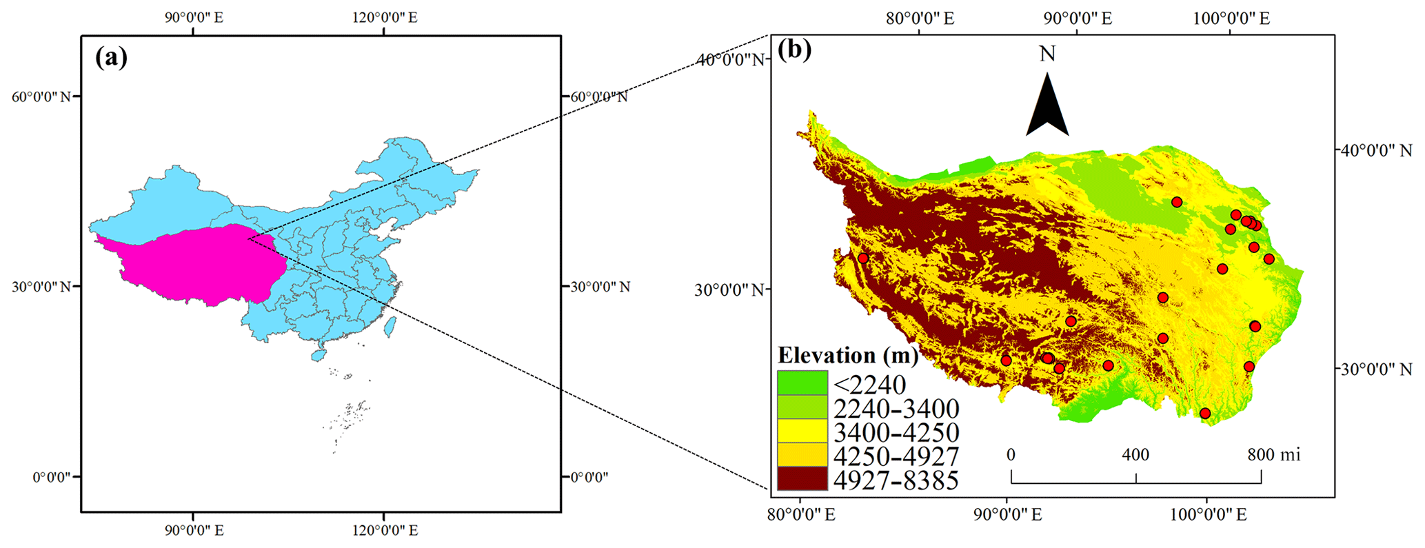
Figure 1The geographical locations and annual mean 8 h O3 concentrations in the ground-observed sites (red dots) over the Tibetan Plateau during 2014–2018. The elevation data are collected from geographical and spatial data cloud at a 30 m spatial resolution.
2.2 Data preparation
2.2.1 Ground-level 8 h O3 concentration
The daily 8 h O3 data in 37 monitoring sites over the Tibetan Plateau from 13 May 2014 to 31 December 2018 were collected from the national air quality monitoring network. The O3 levels in all of these sites were determined using an ultraviolet-spectrophotometry method. The highest 8 h moving average O3 concentration each day was calculated as the daily 8 h O3 level after data quality assurance. The data quality of all the monitoring sites was assured on the basis of the HJ 630-2011 specifications. The data with no more than two consecutive hourly measurements missing in all the days were treated as the valid data.
2.2.2 Satellite-retrieved O3 column amount
The O3 column amounts (DU: total molecules cm−2) during 2005–2018 were downloaded from the Ozone Monitoring Instrument O3 (OMI O3) level-3 data with a 0.25∘ spatial resolution from the website of the National Aeronautics and Space Administration (NASA) (https://acdisc.gsfc.nasa.gov/data/Aura_OMI_Level3/OMDOAO3e.003/, last access: 19 May 2020). The OMI O3 product shows global coverage and traverses the earth once a day. The O3 column amount with a cloud radiance fraction >0.5, terrain reflectivity >30 %, and solar zenith angles >85∘ should be removed. In addition, the cross-track pixels significantly influenced by the row anomaly should be deleted.
2.2.3 Meteorological data and geographical covariates
The daily meteorological data were obtained from ERA-Interim datasets with 0.125∘ resolution. These meteorological data consisted of the 2 m dew-point temperature (d2m), 2 m temperature (t2m), 10 m U wind component (u10), 10 m V wind component (v10), boundary layer height (blh), sunshine duration (sund), surface pressure (sp), and total precipitation (tp). The 30 m resolution elevation data (DEM) were downloaded from the China Resource and Environmental Science Data Center (CRESDC). The data of the gross domestic product (GDP) and population density with 1 km resolution were also extracted from CRESDC. Population density and GDP in 2005, 2010, and 2015 were integrated into the model to predict the surface 8 h O3 concentration over the Tibetan Plateau because these data were available every 5 years. Additionally, the land use data of 30 m resolution (e.g. water, grassland, urban, forest) were also extracted from CRESDC. Lastly, the latitude, longitude, and time were also incorporated into the model.
All of the explanatory variables collected were resampled to 0.25∘ × 0.25∘ grids to predict the O3 level. The original meteorological data with 0.125∘ resolution were resampled to the 0.25∘ grid. The land use area, elevation, GDP, and population density in each grid were calculated using spatial clipping. Lastly, all of the predictors were integrated into an intact table to train the model.
2.3 Model development and assessment
The RF–GAM model was regarded as the hybrid model of RF and GAM. The RF–GAM model was a two-stage model in which the prediction error estimated by the RF model was then simulated by GAM. The prediction results of RF and GAM were summed as the final result of the RF–GAM model (Fig. 2). The detailed equation is as follows:
where Z(s, t) is the estimated 8 h O3 level at the location s and time t, P(s, t) represents the 8 h O3 concentration predicted by the RF model, and E(s, t) denotes the prediction error by GAM.
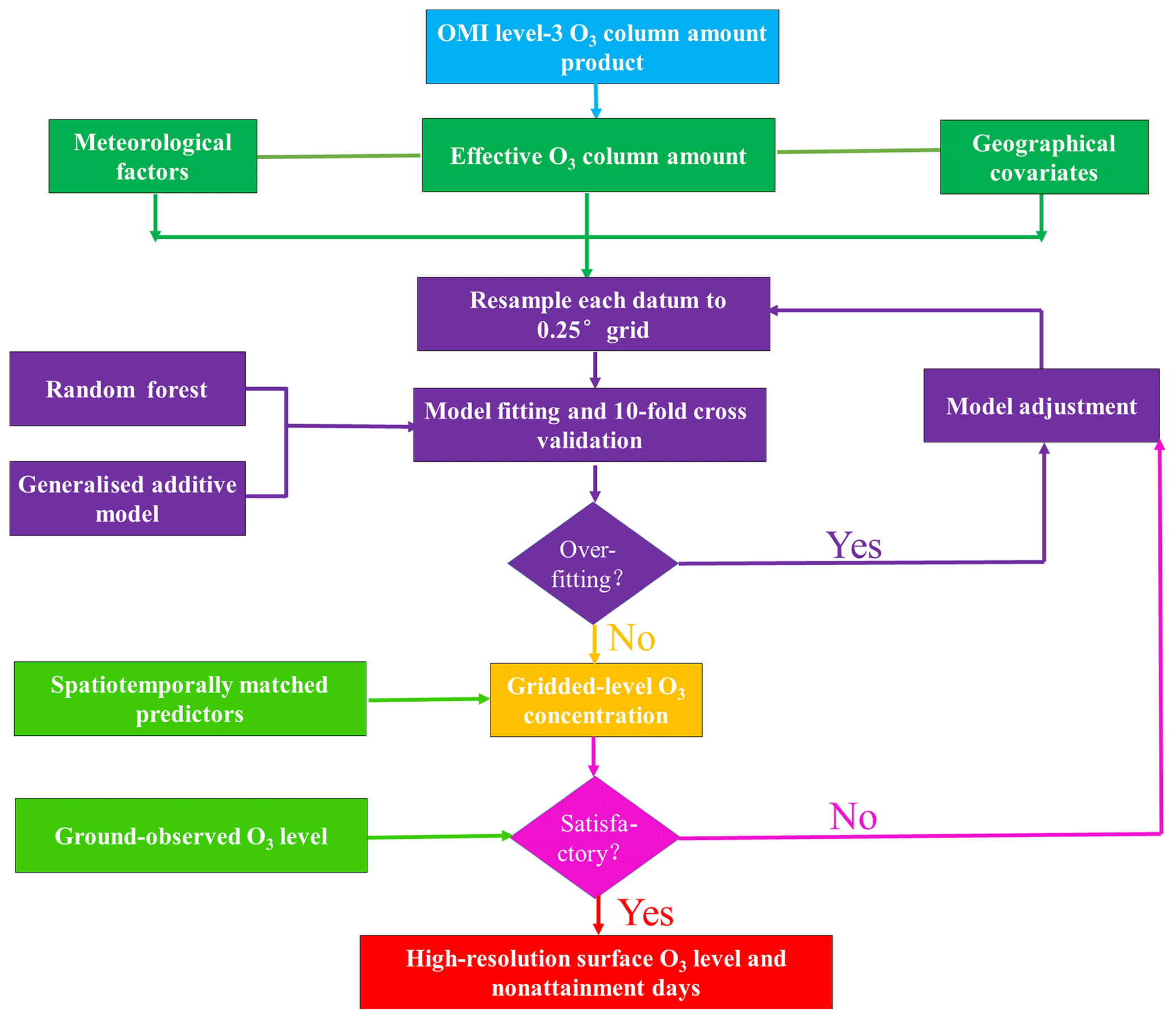

Figure 3Density scatterplots of model fitting and cross-validation results at a daily level. Panels (a), (b), and (c) represent RF–GAM, RF–STK, and RF models, respectively. The red dotted line denotes the fitting linear-regression line. MPE, RMSE, and RPE are mean prediction error (µg m−3), root-mean-square error (µg m−3), and relative percentage error (%), respectively.
In the RF model, a large number of decision trees were planted based on the bootstrap sampling method. At each node of the decision tree, the random samples of all predictors were applied to determine the best split among them. Following the procedure, a simple majority vote was employed to predict the 8 h O3 level. The RF model avoided a priori linear assumption of O3 concentration and predictors, which was often not in good agreement with the actual state. The RF model has two key parameters, including ntree (the number of trees grown) and mtry (the number of explanatory variables sampled for splitting at each node). The prediction performance of the RF model was strongly dependent on the two parameters. The optimal ntree and mtry were determined based on the least out-of-bag (OOB) errors. Based on the iteration result, the optimal ntree and mtry reached 500 and 5, respectively. Besides this, the backward variable selection method was performed on the RF submodel to achieve better performance. At each step of the predictor selection, the variable with the least important value was excluded from the next step. This one-variable-at-a-time exclusion method was repeated until only two explanatory variables remained in the submodel. Finally, all of the selected variables except the area of water were integrated into the model to achieve the best prediction performance. The detailed RF model is as follows:
where O3 denotes the observed 8 h O3 level in the monitoring site; the O3 column represents the O3 column amount in the corresponding grid; Elevation denotes the corresponding elevation of the site; and Agr, Urban, Forest, and Grassland are the agricultural land, urban land, forest land, and the grassland, respectively. Population represents the population density in the corresponding site. Prec, T, WS, P, tsun, and RH are precipitation, air temperature, wind speed, air pressure, sunshine duration, and relative humidity, respectively. Additionally, another five models, including the RF, generalised regression neutral network (GRNN), backward-propagation neural network (BPNN), Elman neural network (ElmanNN), and extreme learning machine (ELM), also used the backward variable selection method. The R2 value was treated as an important parameter for adding or reducing the variable. The variable should be removed when the R2 value of the submodel showed a remarkable decrease with the integration of this variable. Lastly, the optimal variable group was applied to establish the submodel.
Following the RF submodel, the prediction error estimated by the RF submodel was further modelled by the GAM. GAM could reflect the time autocorrelation of the predictive error of RF model, and thus the ensemble model of RF and GAM might decrease the modelling error of the one-stage model. All of the variables were incorporated into the models to establish the second-stage model, and the backward variable selection was also used to determine the optimal variable group.
The 10-fold cross-validation (CV) technique was employed to evaluate the predictive performances for all of the machine-learning models. All of the training datasets were randomly classified into 10 subsets uniformly. In each round of validation, nine subsets were used to train, and the remaining subset was applied to test the model performance. The process was repeated 10 times until every subset has been tested. Some statistical indicators, including the R2, root-mean-square error (RMSE), mean prediction error (MPE), relative percentage error (RPE), and the slope, were calculated to assess the model performance. The optimal model with the best performance was used to estimate the 8 h O3 concentration in recent decades.
Table 1The R2 values, RMSE, MPE, and RPE of RF–GAM in different years during 2014–2018 over the Tibetan Plateau.
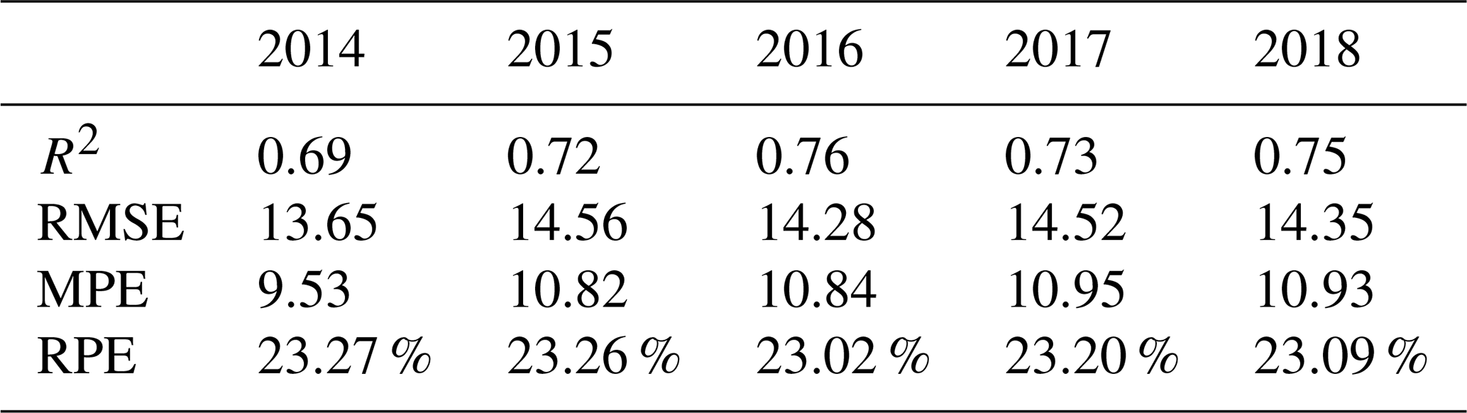
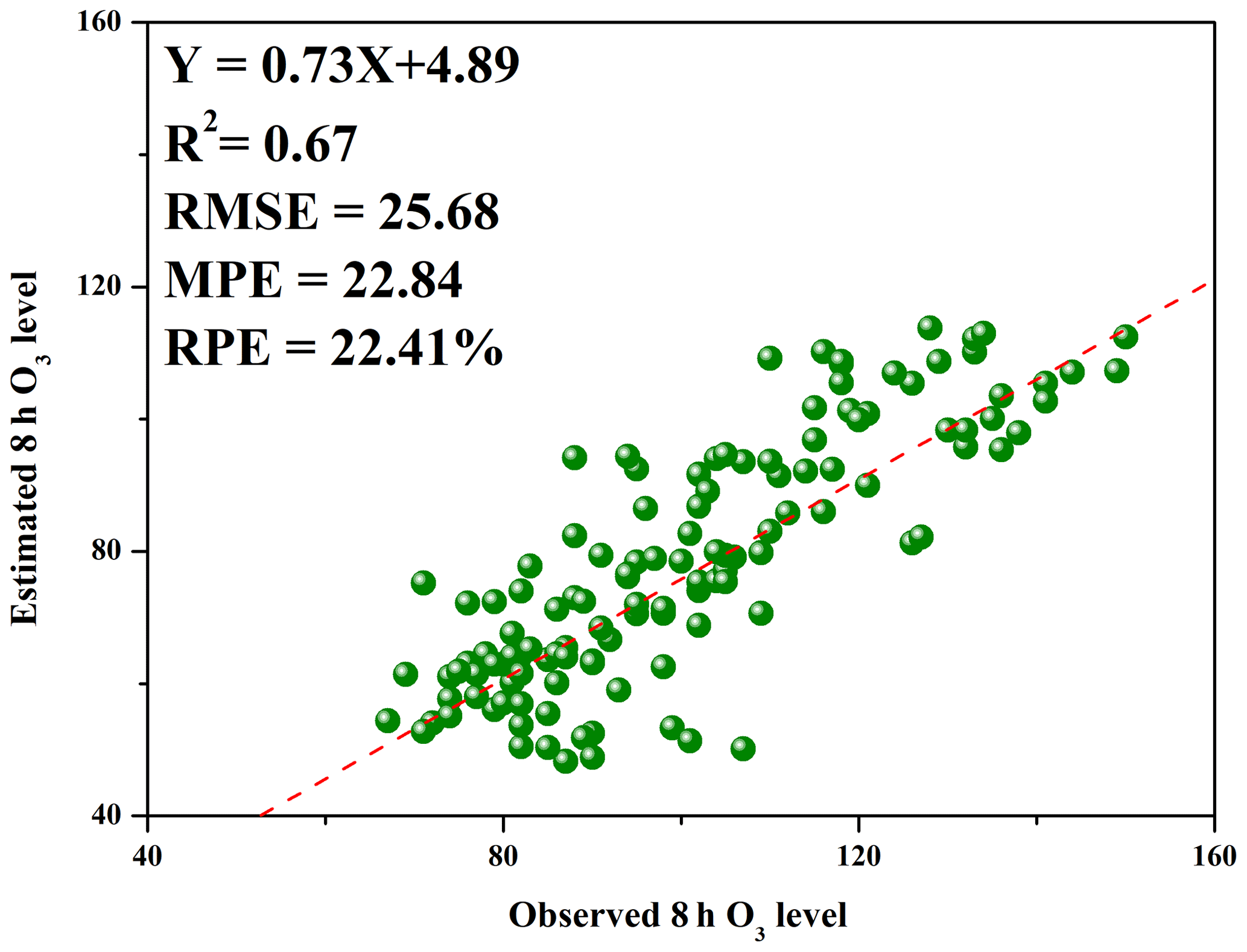
Figure 4The transferring-ability validation of RF–GAM method based on the measured daily 8 h O3 concentration during December 2013–May 2014.

3.1 The validation of model performance
Figures 3 and S2 show the density scatterplots of the fitting and 10-fold cross-validation results for eight machine-learning models for China. The 10-fold cross-validation R2 values followed the order of RF–GAM (R2=0.76)>RF–STK (R2=0.63)>RF (R2=0.55)>GRNN (R2=0.53)>BPNN (R2=0.50)>XGBoost (R2=0.48)>ElmanNN (R2=0.47)>ELM (R2=0.32). The RMSE values of RF–GAM, RF–STK, RF, GRNN, XGBoost, BPNN, ElmanNN, and ELM were 14.41, 17.79, 19.13, 19.41, 20.73, 20.06, 20.61, and 23.36 µg m−3, respectively. Both the MPE and RPE showed similar characteristics to RMSE of the order of RF–GAM (10.97 µg m−3 and 26.50 %) < RF–STK (13.48 µg m−3 and 35.15 %) < RF (14.71 µg m−3 and 35.51 %) < GRNN (14.89 µg m−3 and 35.82 %) < BPNN (15.43 µg m−3 and 36.19 %) < ElmanNN (15.75 µg m−3 and 37.05 %) < XGBoost (15.80 µg m−3 and 38.13 %) < ELM (18.23 µg m−3 and 44.05 %) (Figs. 3 and S2). Besides this, the slope of the RF–GAM model was closer to 1 compared with other models. It was well documented that the RF model generally showed better performance than other models because this method did not need to define complex relationships between the explanatory variables and the O3 concentration (e.g. linear or nonlinear). Furthermore, the variable importance indicators calculated by the RF model can help the user to distinguish the key variables from the noise ones and make full use of the strength of each predictor to assure the model robustness. Although BPNN, GRNN, XGBoost, ElmanNN, and ELM have been widely applied to estimate the air pollutant concentrations (Chen et al., 2018c; Zang et al., 2018; Zhu et al., 2019), these methods suffered from some weaknesses in predicting the pollutant level. For instance, both the BPNN and ElmanNN models could capture the locally optimal solution when the training subsets were integrated into the final model, which decreased the predictive performance of the model (Wang et al., 2015). Moreover, BPNN generally showed slow training speed, especially with the huge training subsets (Li and Park, 2009; Wang et al., 2015). ELM often consumed more computing resources and experienced the overfitting issue due to the increase in sampling size (Huang et al., 2015; Shao et al., 2015). The GRNN method advanced the training speed compared with the BPNN model and avoided the locally optimal solution during the modelling process (Zang et al., 2019), whereas the predictive performance is still worse than that of the RF model. XGBoost was often considered to be robust in predicting the air pollutant level (Li et al., 2020), while the model did not display excellent performance in the present study. This might be attributable to the sampling size in the present study not being big enough because the model generally showed better performance with big samples. Moreover, we found that the two-stage model was superior to the one-way model in the predictive performance. This encouraging result suggested that the relationship between the predictors and the 8 h O3 concentration varied with space and time. The two-stage model used the GAM method to further adjust the prediction error of the RF model and considered the spatiotemporal correlation of the predictor error on the Tibetan Plateau. Although the STK model incorporated space and time into the model simultaneously, the RF–GAM model outperformed the RF–STK model. It was assumed that the STK model showed higher uncertainty in predicting the O3 concentration in regions with few sampling sites (Gao et al., 2016; Li et al., 2017a). Overall, the ensemble RF–GAM model showed significant improvement in predictive performance.
Table 2The R2 values, RMSE, MPE, and RPE of RF–GAM in four seasons over the Tibetan Plateau.
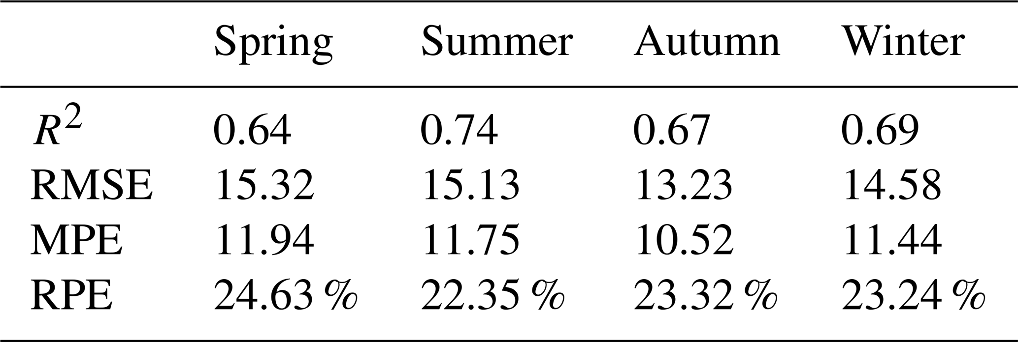
Table 3The predictive performances of RF–GAM in different provinces over the Tibetan Plateau.
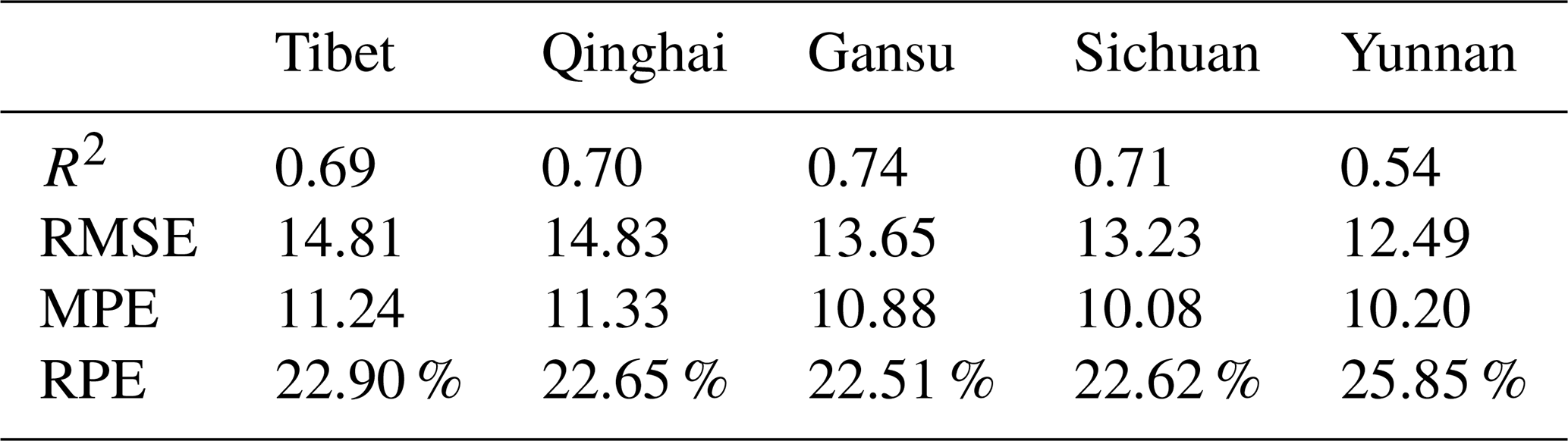
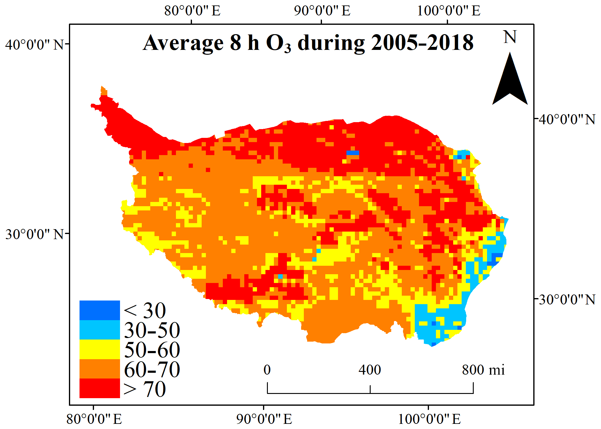
Figure 6The mean value of estimated 8 h O3 concentration during 2005–2018 over the Tibetan Plateau.
The performances of RF–GAM displayed slight differences for each year during 2014–2018. As shown in Table 1, the R2 value showed the highest value (0.76) in 2016, followed by that in 2018 (0.75), 2017 (0.73), and 2015 (0.72), and showed the lowest one in 2014 (0.69). Both the RMSE and MPE exhibited the lowest values in 2014, while these parameters did not show significant variation during 2015–2018. The lowest R2 value and the highest RPE were found in 2014 due to having the lowest sample size, while the highest R2 value and lowest RPE in 2016 were due to the maximum sample size. Geng et al. (2018) found that the predictive performance of the machine-learning model was strongly dependent on the number of training samples and sampling frequency. The lower RMSE and MPE in 2014 might be attributable to the lack of measured O3 data in spring, which decreased the higher value of O3 concentration. The performances of the RF–GAM model in four seasons were also assessed by 10-fold cross validation (Table 2). The predictive performance of the RF–GAM model showed significant seasonal differences, with the highest R2 value observed in summer (0.74), followed by winter (0.69) and autumn (0.67), and the lowest one in spring (0.64). However, both the RMSE and MPE displayed different seasonal characteristics from the R2 value. Both the RMSE and MPE for RF–GAM followed the order of spring (15.32 and 11.94 µg m−3) > summer (15.13 and 11.75 µg m−3) > winter (14.58 and 11.44 µg m−3) > autumn (13.23 and 10.52 µg m−3). The lowest R2 value in spring might be caused by multiple O3 sources and complicate O3 formation mechanisms. On the one hand, the O3 in spring might be generated from the local anthropogenic emission or long-range transport (Li et al., 2017b, 2019b). On the other hand, a strong stratosphere–troposphere exchange process due to the lower height of the troposphere on the Tibetan Plateau might lead to the higher O3 concentration in spring (Skerlak et al., 2014). Unfortunately, both the long-range transport and stratosphere–troposphere exchange process were missing in the RF–GAM model, which restricted the accuracy of O3 estimation in spring. The large estimation errors (e.g. RMSE, MPE, and RPE) in spring and summer were attributable to the high 8 h O3 concentration in these seasons, while the low prediction error observed in autumn was due to the low O3 level.
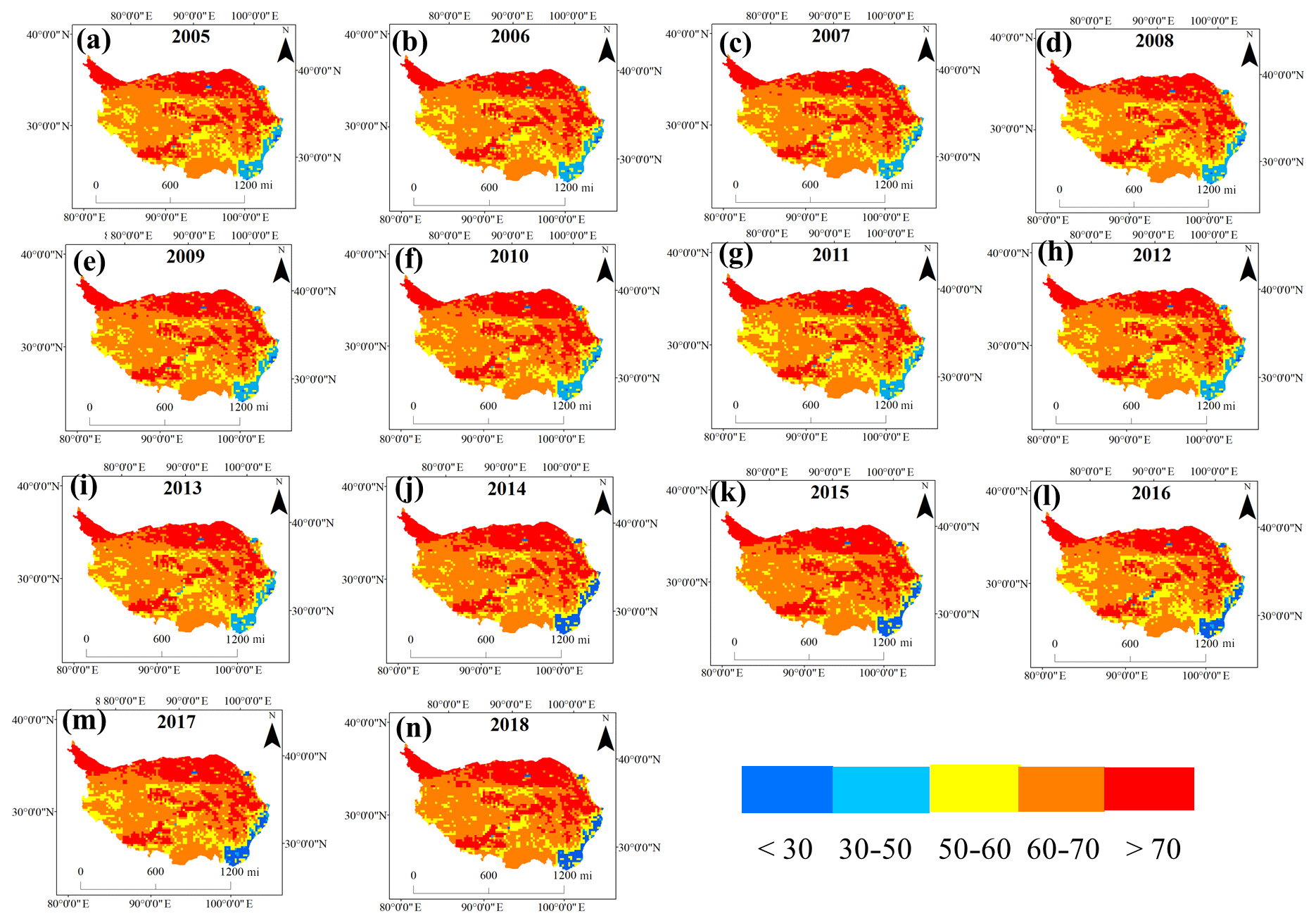
Figure 7The inter-annual variation in predicted 8 h O3 level (µg m−3) from 2005 to 2018 across the Tibetan Plateau.
Apart from the seasonal variation, we also investigated the spatial variabilities in the predictive accuracy for the RF–GAM model. The Tibetan Plateau was classified into five provinces, and then the predictive performance of RF–GAM model in each province was calculated. Among the five provinces, Gansu displayed the highest R2 value (0.74), followed by Sichuan Province (0.71), Qinghai Province (0.70), the autonomous region of Tibet (0.69), and Yunnan Province (0.54) (Table 3). The results shown herein were not in agreement with the previous studies by Geng et al. (2018), who confirmed that the predictive performance of the machine-learning model was positively associated with the sampling size. It was assumed that the spatial distribution of the sampling sites in Tibet was uneven and the sampling density was low, though Tibet possessed the highest number of monitoring sites of the provinces. The prediction errors (RMSE and MPE) did not exhibit the same characteristics as the R2 value. The higher RMSE and MPE were found in the autonomous region of Tibet (14.81 and 11.24 µg m−3) and Qinghai Province (14.83 and 11.33 µg m−3) due to the higher values of blh and sund. The lowest values of the RMSE and MPE could be observed in Yunnan Province, which was due to the higher rainfall amount. The highest RPE was found in Yunnan Province (25.85 %), followed by Tibet (22.90 %), Qinghai (22.65 %), and Sichuan (22.62 %), and the lowest one was found in Gansu Province (22.51 %), which might be linked with the sample size.
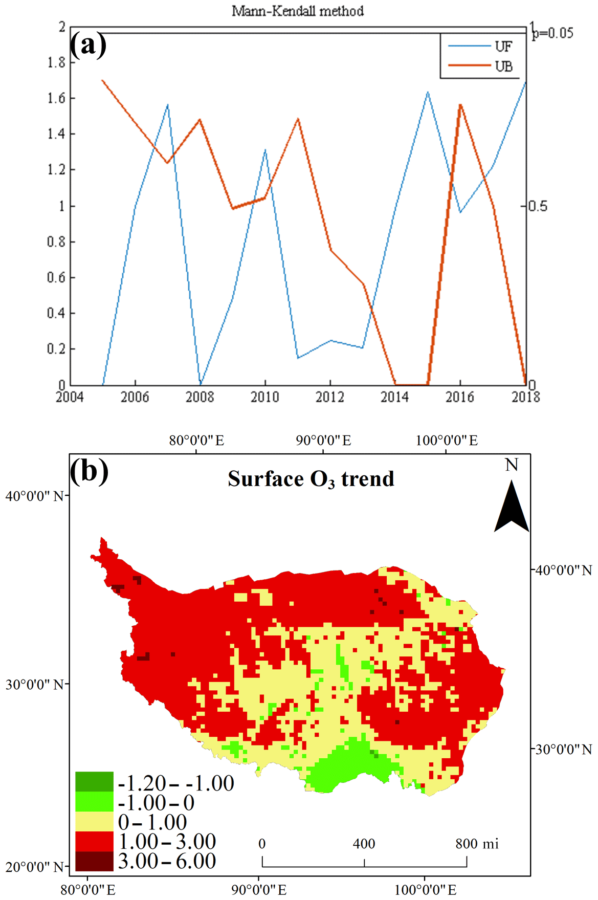
Figure 8The trend analysis of predicted 8 h O3 concentration. Panels (a) and (b) represent the result of Mann–Kendall method and discrepancy of estimated O3 level during 2005–2018 across the Tibetan Plateau.
Although 10-fold cross-validation verified that the RF–GAM model showed better predictive performance in estimating the surface 8 h O3 concentration, the test method cannot validate the transferring ability of the final model. The monitoring site on the Tibetan Plateau before May 2014 is very limited, and only the daily 8 h O3 data in Lhasa from the open-access website (https://www.aqistudy.cn/historydata/daydata.php?city=%E6%8B%89%E8%90%A8&month=2013-12, last access: 19 May 2020) were available to compare with the simulated data. As depicted in Fig. 4, the R2 value of the unlearning 8 h O3 level against the predicted 8 h O3 concentration reached 0.67, which was slightly lower than that of the 10-fold cross-validation R2 value. Overall, the extrapolation ability of the RF–GAM model is satisfactory, and thus it was assumed that the model could be applied to estimate the O3 concentration in other years. Both the RMSE and MPE for the unlearning 8 h O3 level against the predicted 8 h O3 concentration were significantly higher than those of the 10-fold cross validation. It was assumed that Lhasa showed a higher surface 8 h O3 concentration over the Tibetan Plateau.
To date, some previous studies also simulated the surface O3 concentration on the Tibetan Plateau using statistical models (Zhan et al., 2018). For instance, Zhan et al. (2018) employed the RF–STK model to estimate the surface O3 concentration over China and explained the 66 % spatial variability in the O3 level on the Tibetan Plateau. Apart from these statistical models, some classical CTMs were also applied to estimate the O3 concentration in remote areas. Both Liu et al. (2018) and Lin et al. (2018) used CMAQ to estimate the O3 level across China, while the R2 values in most of cities were lower than 0.50. In terms of the predictive performance, the RF–GAM model in our study showed significant advantages compared with previous studies. It should be noted that our RF–GAM model could outperform most of current models, chiefly because of (1) accounting for the temporal autocorrelation of the surface O3 concentration and (2) the use of high-quality satellite data.
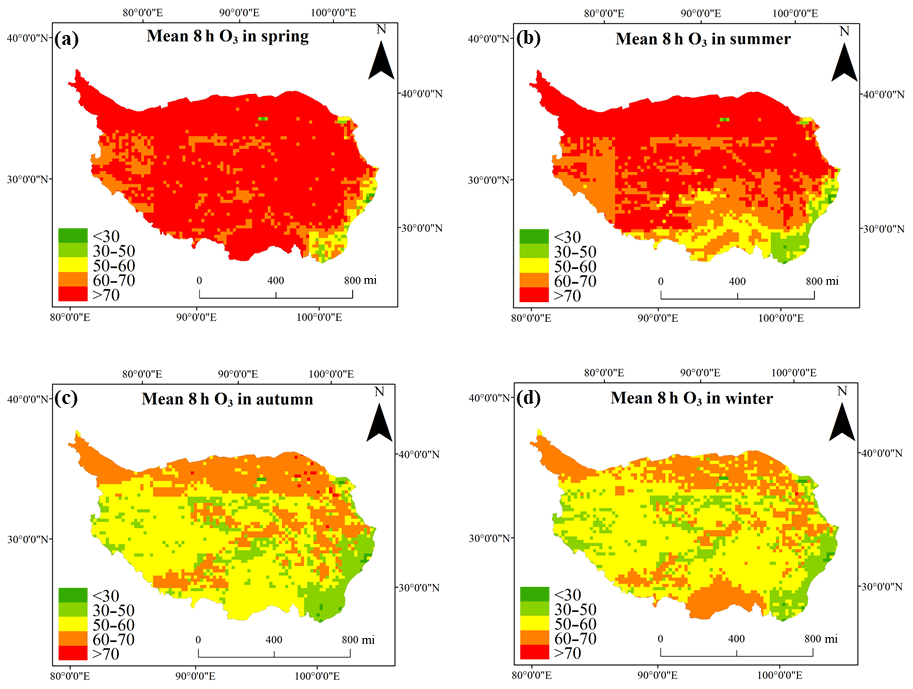
Figure 9The seasonal variability in estimated 8 h O3 level across the Tibetan Plateau. Panels (a–d) represent the predicted 8 h O3 concentrations in spring, summer, autumn, and winter, respectively.
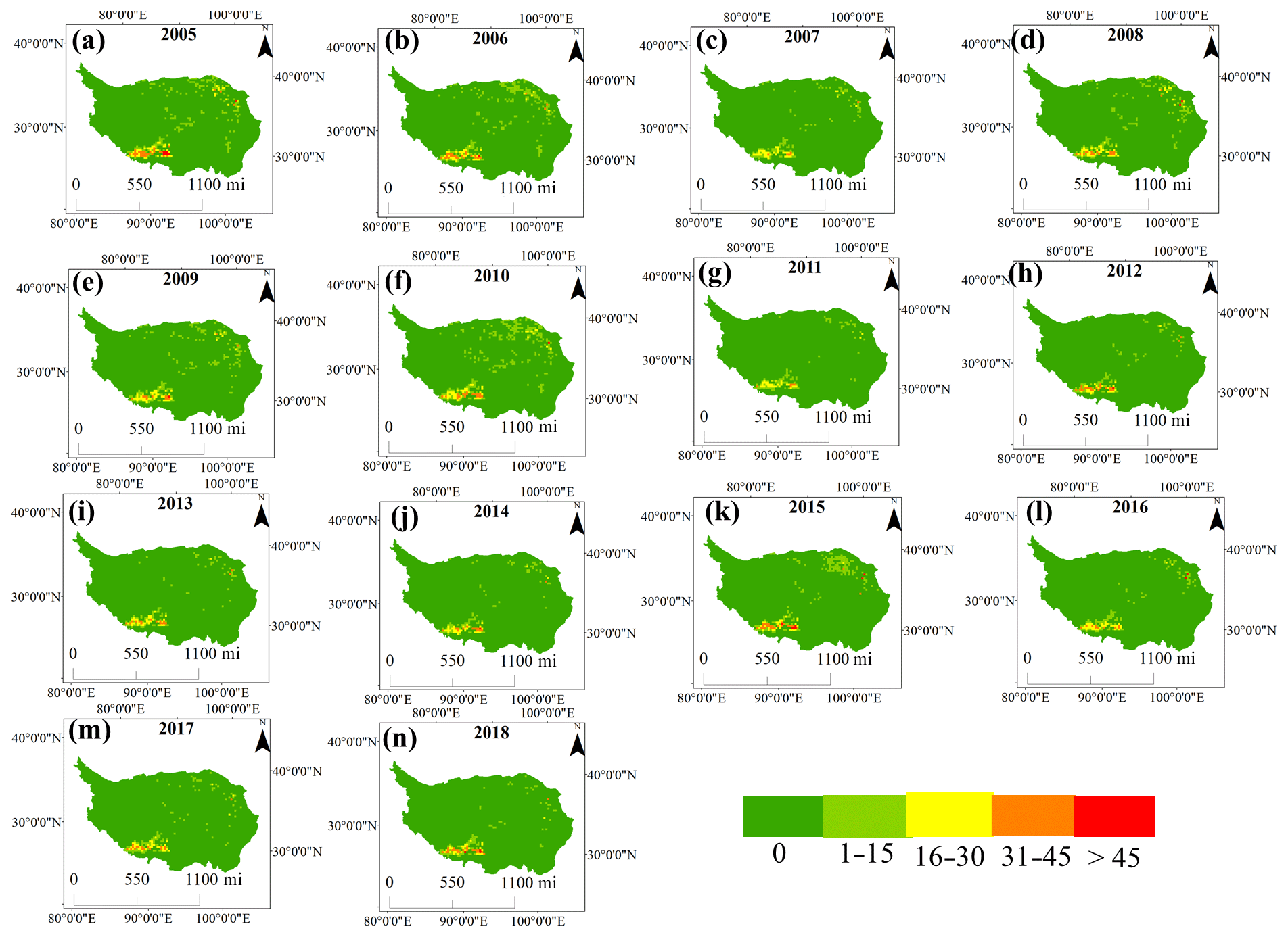
Figure 10The spatial distributions of nonattainment days on the Tibetan Plateau during 2005–2018.
3.2 Variable importance
The results of variable importance for key variables are depicted in Fig. 5. In the final RF–GAM model, it was found that time was the dominant factor for the 8 h O3 concentration on the Tibetan Plateau, indicating that the ambient O3 concentration displayed significant temporal correlation. Following the time, meteorological factors served as the main factors for the O3 pollution in remote regions. The sum of sund, sp, d2m, t2m, and tp constituted 34.43 % of the overall variable importance. Among others, sund was considered to be the most important meteorological factor for the O3 pollution. It was assumed that strong solar radiation and long duration of sunshine favoured the photochemical generation of ambient O3 (Malik and Tauler, 2015; Stähle et al., 2018). Tan et al. (2018) demonstrated that the chemical reaction between NOx and VOCs was strongly dependent on the sunlight. Besides this, the atmospheric pressure (sp) was also treated as a major driver for the O3 pollution over the Tibetan Plateau. Santurtún et al. (2015) have demonstrated that sp was closely linked to the atmospheric circulation and synoptic-scale meteorological pattern, which could influence the long-range transport of ambient O3. Apart from sund and sp, d2m and t2m played significant role in the O3 pollution, which was consistent with many previous studies (Zhan et al., 2018). Zhan et al. (2018) observed that cold temperatures were not favourable to the O3 formation. d2m can affect the surface O3 pollution through two aspects. On the one hand, RH affected heterogeneous reactions of O3 and particles (e.g. soot, mineral) (He et al., 2017; He and Zhang, 2019; Yu, 2019). On the other hand, high RH could increase the soil moisture and evaporation, and thus the water-stressed plants tended to emit more biogenic isoprene, thereby promoting the elevation of O3 concentration (Zhang and Wang, 2016). It should be noted that the effect of precipitation on O3 pollution was weaker than those of other meteorological factors. Zhan et al. (2018) also found a similar result and believed that rain scavenging served as the key pathway for the O3 removal only when O3 pollution was very serious. The effect of the O3 column amount on surface O3 concentration seemed to be lower than those of most meteorological factors, suggesting that vertical transport of ambient O3 was complex. Although socioeconomic factors and land use types were not dominant factors for the O3 pollution on the Tibetan Plateau, they still cannot be ignored in the present study because the predictive performance would worsen if these variables were excluded from the model. It was widely acknowledged that the anthropogenic emissions focused on developed urban areas with high population density, especially on the remote plateau (Zhang et al., 2007; Zheng et al., 2017). Compared with the urban land, the grassland played a more important role in the O3 pollution on the Tibetan Plateau. It was thus assumed that the grassland was widely distributed on the Tibetan Plateau, which could release a large amount of biogenic volatile organic compounds (BVOCs) (Fang et al., 2015). It was well known that photochemical reactions of BVOCs and NOx in the presence of sunlight caused the O3 formation (Calfapietra et al., 2013; Yu et al., 2006). Furthermore, Fang et al. (2015) confirmed that BVOC emission on the Tibetan Plateau displayed a remarkable increase in the wet seasons.
3.3 The spatial distribution of estimated 8 h O3 concentration over the Tibetan Plateau
Figure 6 depicts the spatial distribution of the 8 h O3 level estimated by the novel RF–GAM model. The spatial distribution pattern modelled by the RF–GAM model showed a similar characteristic to the results found by previous studies except on the northern Tibetan Plateau (Liu et al., 2018). The estimated 8 h O3 concentration displayed the highest value in some cities of the northern Tibetan Plateau, such as Huangnan (73.48±4.53 µg m−3) and Hainan (72.24±5.34 µg m−3), followed by the cities in the central region, including Lhasa (65.99±7.24 µg m−3) and Shigatse (65.15±6.14 µg m−3), and the lowest one was found in a city of the southeastern Tibetan Plateau (Aba) (55.17±12.77 µg m−3). The spatial pattern of the 8 h O3 concentration is highly consistent with the result predicted by Liu et al. (2018) using the CMAQ model, while it is not in agreement with the result estimated by Zhan et al. (2018) using the RF–STK model. The difference between the present study and Zhan et al. (2018) is seen on the northern Tibetan Plateau, which lacks a monitoring site and still has the higher uncertainty. Firstly, this might be due to the weakness of RF–STK mentioned above. Moreover, Zhan et al. (2018) only used the ground-level-measured data in 2015 to establish the model, and the data from new sites since 2015 were not incorporated into the model, which could increase the model uncertainty (Zhan et al., 2018). As shown in Fig. 6, most of the cities in Qinghai Province (e.g. Huangnan, Hainan, and Guoluo) generally showed a higher 8 h O3 concentration over the Tibetan Plateau, which was in a good agreement with the spatial distribution of the O3 column amount (Fig. S3). Besides this, some cities in Tibet, such as Shigatse and Lhasa, also showed higher 8 h O3 levels. It was assumed that the precursor emissions in these regions were significantly higher than those in other cities of the Tibetan Plateau (Fig. S4). Zhang et al. (2007) used the satellite data to observe that the higher VOCs and NOx emission was concentrated in the residential areas with high population density on the remote Tibetan Plateau. Apart from the effect of anthropogenic emission, the meteorological conditions could also be important factors for the 8 h O3 concentration. As shown in Figs. S5–S10, a higher blh and sp on the northeastern Tibetan Plateau might promote the O3 formation through the reaction of the VOC and OH radical, leading to a higher 8 h O3 concentration in these cities (Ou et al., 2015). In addition, a lower tp occurred on the northern Tibetan Plateau and the northeastern Tibetan Plateau, both of which were unfavourable to the ambient O3 removal (Yoo et al., 2014). In contrast, the higher tp observed on the southeastern Tibetan Plateau resulted in slight O3 pollution.
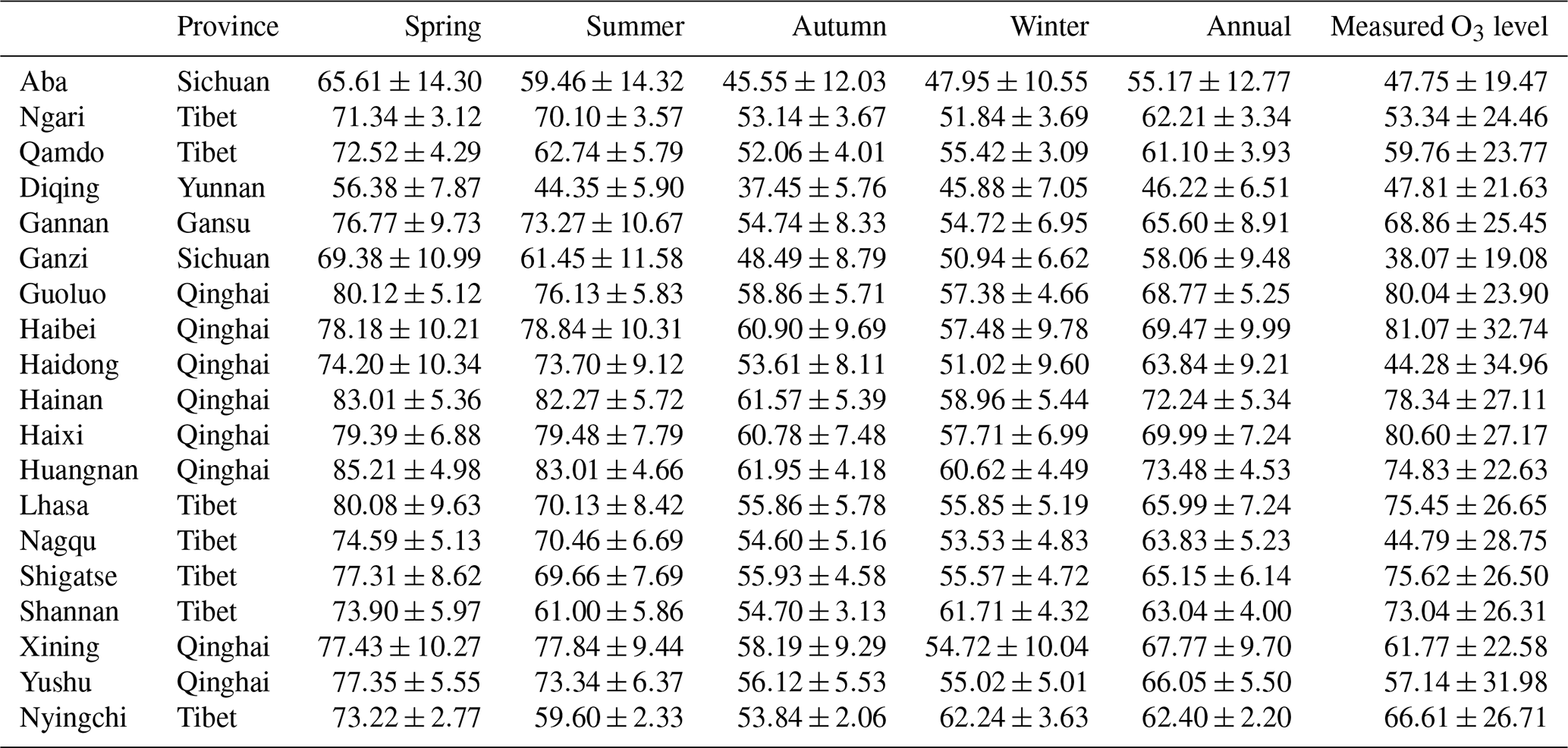
Table 4The estimated 8 h O3 concentration in 19 prefecture-level cities over the Tibetan Plateau during four seasons, including spring, summer, autumn, and winter.
3.4 The temporal variation in the simulated 8 h O3 concentration over the Tibetan Plateau
The annual mean estimated 8 h O3 concentration on the Tibetan Plateau displayed a slow increase, from 64.74±8.30 to 66.45±8.67 µg m−3 in 2005–2015 (Table S1), whereas it decreased from the peak to 65.87±8.52 µg m−3 during 2015–2018 (Fig. 7). Based on the Mann–Kendall method (Fig. 8a), it was found that the surface O3 concentration exhibited a slight increase on the whole, while the degree of increase was not significant (p>0.05). Besides this, it should be noted that the O3 concentrations in various regions showed different rates of increase. As depicted in Fig. 8b, we found that the 8 h O3 concentrations on the northern, western, and eastern Tibetan Plateau displayed significant an increasing trend at the rate of 1–3 µg m−3 during 2005–2018. The middle region of the Tibetan Plateau showed a moderate increase trend at the rate of 0–1 µg m−3. However, the 8 h O3 concentration in Shigatse and Shannan even displayed a decreasing trend in 2005–2018.
Besides this, the 8 h O3 concentrations on the Tibetan Plateau displayed significantly seasonal discrepancy. The estimated 8 h O3 level on the Tibetan Plateau followed the order of spring (75.00±8.56 µg m−3) > summer (71.05±11.13 µg m−3) > winter (56.39±7.42 µg m−3) > autumn (56.13±8.27 µg m−3) (Fig. 9 and Table 4). The 8 h O3 concentrations in most of prefecture-level cities showed similar seasonal characteristics, with overall seasonal variation on the Tibetan Plateau. Based on the result summarised in Table S2, it was found that the key precursors of ambient O3 generally displayed higher emissions in winter compared with other seasons. However, the seasonal distribution of ambient O3 concentration was not in accordance with the precursor emissions, suggesting that the meteorological factors might play more important roles in ambient O3 concentration. It was well known that the higher air temperatures in spring and summer were closely related to the low sp and high sund, both of which promoted O3 formation (Sitnov et al., 2017). Although summer showed the highest air temperature and the longest sunshine duration, the higher rainfall amount in summer decreased the ambient O3 concentration via wet deposition (Li et al., 2017a, 2019b). Moreover, the highest blh occurred in spring, which was favourable to the strong stratosphere–troposphere exchange process on the Tibetan Plateau (Skerlak et al., 2014). Therefore, the 8 h O3 concentrations in summer and winter were lower than that in spring. Nonetheless, the 8 h O3 levels in Diqing, Shannan, and Nyingchi displayed the highest values in spring (56.38±7.87, 73.90±5.97, and 73.22±2.77 µg m−3), followed by winter (45.88±7.05, 61.71±4.32, and 62.24±3.63 µg m−3) and summer (44.35±5.90, 61.00±5.86, and 59.60±2.33 µg m−3), and the lowest ones in autumn (37.45±5.76, 54.70±3.13, and 53.84±2.06 µg m−3). The lower O3 level in summer than winter was mainly attributable to the higher precipitation observed in the summer of these cities (Fig. S11). In addition, it should be noted that the NOx and VOC emissions of the southern Tibetan Plateau (e.g. Shannan) exhibited higher values in winter compared with other seasons.
3.5 The nonattainment days over the Tibetan Plateau during 2005–2018
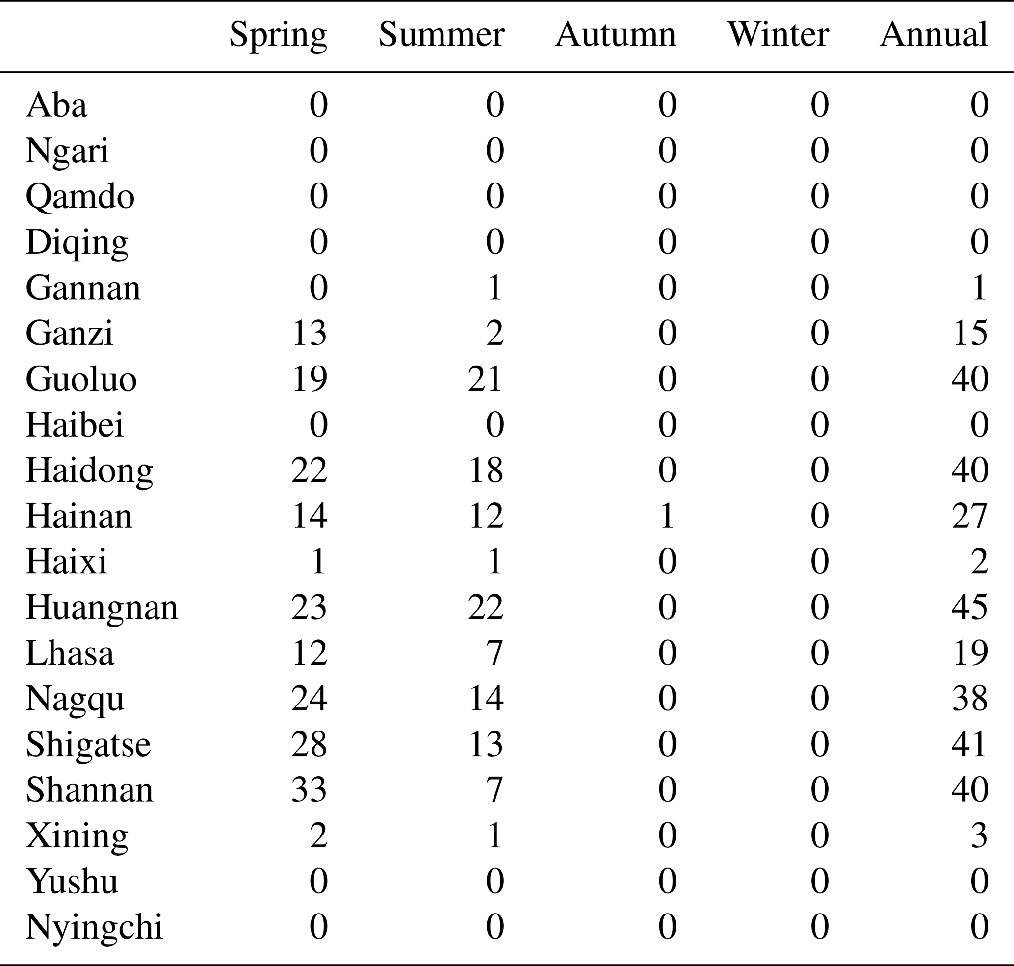
The annual mean nonattainment days in the 19 prefecture-level cities over the Tibetan Plateau are summarised in Table 2. The value of 100 µg m−3 was regarded as the critical value for the 8 h O3 level by the World Health Organization (WHO). Nonattainment days refer to total days with the 8 h O3 concentration higher than 100 µg m−3. Although the annual mean 8 h O3 concentrations in all of the cities over the Tibetan Plateau did not exceed the critical value, not all of the regions experienced excellent air quality in the long term (2005–2018). Some cities of Qinghai Province, including Huangnan, Haidong, and Guoluo, suffered from 45, 40, and 40 nonattainment days each year (Fig. 10 and Table 5). Besides this, some cities on the southern Tibetan Plateau, such as Shigatse and Shannan, also experienced more than 40 nonattainment days each year, suggesting that the Tibetan Plateau still faced the risk of O3 pollution. Fortunately, some remote cities, such as Ali, Ngari, and Qamdo, did not experience excessive O3 pollution all the time, which was ascribed to low precursor emissions and appropriate meteorological conditions. It should be noted that the nonattainment days in regions with high O3 concentration showed significant seasonal difference, whereas the seasonal difference was not remarkable in cities with low O3 pollution. As shown in Table 2, it should be noted that nearly all of the nonattainment days could be detected in spring and summer, which was in good agreement with the O3 levels in different seasons, indicating that the O3 pollution issue should be given more attention in spring and summer.
Table 5The mean nonattainment days (8 h O3 level >100 µg m−3) in 19 prefecture-level cities over the Tibetan Plateau each year.
The determination of nonattainment days showed some uncertainties, owing to the predictive error of modelled O3 concentration. First of all, meteorological data used in RF–GAM model were collected from reanalysis data, and these gridded data often showed some uncertainties, which could increase the uncertainty of O3 estimation. Second, the O3 column amount used in the present study reflected the vertical O3 column amount rather than the surface O3 concentration. Thus, it could decrease the predictive performance of the surface O3 level.
In the present study, we developed a novel hybrid model (RF–GAM) based on multiple explanatory variables to estimate the surface 8 h O3 concentration across the remote Tibetan Plateau. The 10-fold cross-validation method demonstrated that RF–GAM achieved excellent performance, with the highest R2 value (0.76) and lowest root-mean-square error (RMSE) (14.41 µg m−3), compared with other models, including the RF–STK, RF, BPNN, XGBoost, GRNN, ElmanNN, and ELM models. Moreover, the unlearning ground-level-measured O3 data validated the fact that the RF–GAM model showed better extrapolation performance (R2=0.67, RMSE =25.68 µg m−3). The result of variable importance suggested that time, sund, and sp were key factors for the surface 8 h O3 concentration over the Tibetan Plateau. Based on the RF–GAM model, we found that the estimated 8 h O3 concentration exhibited notable spatial variation, with higher values in some cities of the northern Tibetan Plateau, such as Huangnan (73.48±4.53 µg m−3) and Hainan (72.24±5.34 µg m−3), and lower values in some cities of the southeastern Tibetan Plateau, such as Aba (55.17±12.77 µg m−3). Besides this, we also found that the O3 level displayed a slow increase, from 64.74±8.30 to 66.45±8.67 µg m−3 from 2005 to 2015, while the O3 concentration decreased to 65.87±8.52 µg m−3 in 2018. The estimated 8 h O3 level on the Tibetan Plateau showed significant seasonal discrepancy in the order of spring (75.00±8.56 µg m−3) > summer (71.05±11.13 µg m−3) > winter (56.39±7.42 µg m−3) > autumn (56.13±8.27 µg m−3). Based on the critical value set by the WHO, most of the cities on the Tibetan Plateau had excellent air quality, while several cities (e.g. Huangnan, Haidong, and Guoluo) still suffered from more than 40 nonattainment days each year.
The RF–GAM model for O3 estimation has several limitations. First of all, the O3 estimation of the northern Tibetan Plateau might show some uncertainties because there are few ground-level monitoring sites, and thus we cannot validate the reliability of predicted values in regions without a monitoring site. Secondly, our approach did not include data on the emission inventory or traffic count because the continuous emissions of NOx and VOCs were not open access. Lastly, we only focused on the temporal variation in the surface O3 concentration in the past 10 years, and the short-term O3 data cannot reflect the response of O3 pollution to climate change. In the future work, we should combine more explanatory variables such as long-term NOx and VOC emissions to retrieve the surface O3 level over the Tibetan Plateau in recent decades.
The daily O3 column data were collected from https://acdisc.gsfc.nasa.gov/data/Aura_OMI_Level3/OMDOAO3e.003/2005/ (GES DISC, 2020). The ground-observed O3 data were downloaded from https://www.aqistudy.cn/historydata/ (Aqistudy, 2020). All of these data are open access.
The supplement related to this article is available online at: https://doi.org/10.5194/acp-20-6159-2020-supplement.
This study was conceived by RL and HF. Statistical modelling was performed by RL, YZ, YM, WZ, and ZZ. RL drafted the paper.
The authors declare that they have no conflict of interest.
This article is part of the special issue “Study of ozone, aerosols and radiation over the Tibetan Plateau (SOAR-TP) (ACP/AMT inter-journal SI)”. It is not associated with a conference.
This work has been supported by the National Natural Science Foundation of China (grant nos. 91744205, 21777025, 21577022, 21177026).
This research has been supported by the National Natural Science Foundation of China (grant no. 91744205).
This paper was edited by Tao Wang and reviewed by two anonymous referees.
Aqistudy: Ground-observed daily O3 data, available at: https://www.aqistudy.cn/historydata/, last access: 20 May 2020.
Bornman, J. F., Barnes, P. W., Robson, T. M., Robinson, S. A., Jansen, M. A., Ballaré, C. L., and Flint, S. D.: Linkages between stratospheric ozone, UV radiation and climate change and their implications for terrestrial ecosystems, Photoch. Photobio. Sci, 18, 681–716, https://doi.org/10.1039/C8PP90061B, 2019.
Calfapietra, C., Fares, S., Manes, F., Morani, A., Sgrigna, G., and Loreto, F.: Role of Biogenic Volatile Organic Compounds (BVOC) emitted by urban trees on ozone concentration in cities: A review, Environ. Pollut., 183, 71–80, https://doi.org/10.1016/j.envpol.2013.03.012, 2013.
Chan, C., Wong, K., Li, Y., Chan, L., and Zheng, X.: The effects of Southeast Asia fire activities on tropospheric ozone, trace gases and aerosols at a remote site over the Tibetan Plateau of Southwest China, Tellus B, 58, 310–318, https://doi.org/10.1111/j.1600-0889.2006.00187.x, 2006.
Chen, G., Knibbs, L. D., Zhang, W., Li, S., Cao, W., Guo, J., Ren, H., Wang, B., Wang, H., and Williams, G.: Estimating spatiotemporal distribution of PM1 concentrations in China with satellite remote sensing, meteorology, and land use information, Environ. Pollut., 233, 1086–1094, https://doi.org/10.1016/j.envpol.2017.10.011, 2018a.
Chen, G., Li, S., Knibbs, L. D., Hamm, N., Cao, W., Li, T., Guo, J., Ren, H., Abramson, M. J., and Guo, Y.: A machine learning method to estimate PM2.5 concentrations across China with remote sensing, meteorological and land use information, Sci. Total Environ. 636, 52–60, https://doi.org/10.1016/j.scitotenv.2018.04.251, 2018b.
Chen, G., Morawska, L., Zhang, W., Li, S., Cao, W., Ren, H., Wang, B., Wang, H., Knibbs, L. D., and Williams, G.: Spatiotemporal variation of PM1 pollution in China, Atmos. Environ., 178, 198–205, https://doi.org/10.1016/j.atmosenv.2018.01.053, 2018c.
Chen, P., Yang, J., Pu, T., Li, C., Guo, J., Tripathee, L., and Kang, S.: Spatial and temporal variations of gaseous and particulate pollutants in six sites in Tibet, China, during 2016–2017, Aerosol Air Qual. Res., 19, 516–527, https://doi.org/10.4209/aaqr.2018.10.0360, 2019.
Emberson, L. D., Pleijel, H., Ainsworth, E. A., Berg, M. V. D., Ren, W., Osborne, S., Mills, G., Pandey, D., Dentener, F., Buker, P., Ewert, F., Koeble, R., and Dingenen, R. V.: Ozone effects on crops and consideration in crop models, Eur. J. Agron., 100, 19–34, https://doi.org/10.1016/j.eja.2018.06.002, 2018.
Fang, K., Makkonen, R., Guo, Z., Zhao, Y., and Seppä, H.: An increase in the biogenic aerosol concentration as a contributing factor to the recent wetting trend in Tibetan Plateau, Sci. Rep., 5, 14628, https://doi.org/10.1038/srep14628, 2015.
Feng, Z., Hu, E., Wang, X., Jiang, L., and Liu, X.: Ground-level O3 pollution and its impacts on food crops in China: a review, Environ. Pollut., 199, 42–48, https://doi.org/10.1016/j.envpol.2015.01.016, 2015.
Feng, Z., De Marco, A., Anav, A., Gualtieri, M., Sicard, P., Tian, H., Fornasier, F., Tao, F., Guo, A., and Paoletti, E.: Economic losses due to ozone impacts on human health, forest productivity and crop yield across China, Environ. Interna, 131, 104966, https://doi.org/10.1016/j.envint.2019.104966, 2019.
Fioletov, V., Bodeker, G., Miller, A., McPeters, R., and Stolarski, R.: Global and zonal total ozone variations estimated from ground-based and satellite measurements: 1964–2000, J. Geophys. Res., 107, ACH 21-21–ACH 21-14, https://doi.org/10.1029/2001JD001350, 2002.
Fu, Y., Liao, H., and Yang, Y.: Interannual and decadal changes in tropospheric ozone in China and the associated chemistry-climate interactions: A review, Adv. Atmos. Sci., 36, 975–993, https://doi.org/10.1007/s00376-019-8216-9, 2019.
Gao, Z., Shao, X., Jiang, P., Cao, L., Zhou, Q., Yue, C., Liu, Y., and Wang, C.: Parameters optimization of hybrid fiber laser-arc butt welding on 316L stainless steel using Kriging model and GA, Opt. Laser Technol., 83, 153–162, https://doi.org/10.1016/j.optlastec.2016.04.001, 2016.
Geng, G., Murray, N. L., Chang, H. H., and Liu, Y.: The sensitivity of satellite-based PM2.5 estimates to its inputs: Implications to model development in data-poor regions, Environ. Interna., 121, 550–560, https://doi.org/10.1016/j.envint.2018.09.051, 2018.
GES DISC: Daily O3 column data, available at: https://acdisc.gsfc.nasa.gov/data/Aura_OMI_Level3/OMDOAO3e.003/2005/, last access: 20 May 2020.
Ghude, S. D., Chate, D., Jena, C., Beig, G., Kumar, R., Barth, M., Pfister, G., Fadnavis, S., and Pithani, P.: Premature mortality in India due to PM2.5 and ozone exposure, Geophys. Res. Lett., 43, 4650–4658, https://doi.org/10.1002/2016GL068949, 2016.
He, X., Pang, S., Ma, J., Zhang, Y.: Influence of relative humidity on heterogeneous reactions of O3 and O3∕SO2 with soot particles: potential for environmental and health effects, Atmos. Environ., 165, 198–206, https://doi.org/10.1016/j.atmosenv.2017.06.049, 2017.
He, X. and Zhang, Y.-H.: Influence of relative humidity on SO2 oxidation by O3 and NO2 on the surface of TiO2 particles: Potential for formation of secondary sulfate aerosol, Spectrochim. Acta A, 219, 121–128, https://doi.org/10.1016/j.saa.2019.04.046, 2019.
Huang, G., Huang, G.-B., Song, S., and You, K.: Trends in extreme learning machines: A review, Neural Networks, 61, 32–48, https://doi.org/10.1016/j.neunet.2014.10.001, 2015.
Kim, S.-Y., Bechle, M., Hankey, S., Sheppard, E. L. A., Szpiro, A. A., and Marshall, J. D.: Concentrations of criteria pollutants in the contiguous US, 1979–2015: Role of model parsimony in integrated empirical geographic regression, UW Biostatistics Working Paper Series, 2018.
Li, C. H. and Park, S. C.: Combination of modified BPNN algorithms and an efficient feature selection method for text categorization, Inform. Process Manag., 45, 329–340, https://doi.org/10.1016/j.ipm.2008.09.004, 2009.
Li, H., Liu, T., Wang, M., Zhao, D., Qiao, A., Wang, X., Gu, J., Li, Z., and Zhu, B.: Design optimization of stent and its dilatation balloon using kriging surrogate model, Biomed. Eng. Online, 16, 13, https://doi.org/10.1186/s12938-016-0307-6, 2017a.
Li, J., Mao, J., Fiore, A. M., Cohen, R. C., Crounse, J. D., Teng, A. P., Wennberg, P. O., Lee, B. H., Lopez-Hilfiker, F. D., Thornton, J. A., Peischl, J., Pollack, I. B., Ryerson, T. B., Veres, P., Roberts, J. M., Neuman, J. A., Nowak, J. B., Wolfe, G. M., Hanisco, T. F., Fried, A., Singh, H. B., Dibb, J., Paulot, F., and Horowitz, L. W.: Decadal changes in summertime reactive oxidized nitrogen and surface ozone over the Southeast United States, Atmos. Chem. Phys., 18, 2341–2361, https://doi.org/10.5194/acp-18-2341-2018, 2018.
Li, R., Cui, L., Li, J., Zhao, A., Fu, H., Wu, Y., Zhang, L., Kong, L., and Chen, J.: Spatial and temporal variation of particulate matter and gaseous pollutants in China during 2014–2016, Atmos. Environ, 161, 235–246, https://doi.org/10.1016/j.atmosenv.2017.05.008, 2017b.
Li, R., Cui, L., Meng, Y., Zhao, Y., and Fu, H.: Satellite-based prediction of daily SO2 exposure across China using a high-quality random forest-spatiotemporal Kriging (RF-STK) model for health risk assessment, Atmos. Environ, 208, 10–19, https://doi.org/10.1016/j.atmosenv.2019.03.029, 2019a.
Li, R., Wang, Z., Cui, L., Fu, H., Zhang, L., Kong, L., Chen, W., and Chen, J.: Air pollution characteristics in China during 2015–2016: Spatiotemporal variations and key meteorological factors, Sci. Total Environ., 648, 902–915, https://doi.org/10.1016/j.scitotenv.2018.08.181, 2019b.
Li, R., Cui, L. L, Fu, H. B., Li, J. L., Zhao, Y. L., and Chen, J. M.: Satellite-based estimation of full-coverage ozone (O3) concentration and health effect assessment across Hainan Island, J. Clean Prod., 244, 118773, https://doi.org/10.1016/j.jclepro.2019.118773, 2020.
Lin, W., Zhu, T., Song, Y., Zou, H., Tang, M., Tang, X., and Hu, J.: Photolysis of surface O3 and production potential of OH radicals in the atmosphere over the Tibetan Plateau, J. Geophys. Res., 113, D02309, https://doi.org/10.1029/2007JD008831, 2008.
Lin, Y. Y., Jiang, F., Zhao, J., Zhu, G., He, X. J., Ma, X. L., Li, S., Sabel, C. E., and Wang, H. K.: Impacts of O3 on premature mortality and crop yield loss across China, Atmos. Environ., 194, 41–47, https://doi.org/10.1016/j.atmosenv.2018.09.024, 2018.
Liu, H., Liu, S., Xue, B. R., Lv, Z. F., Meng, Z. H., Yang, X. F., Xue, T., Yu, Q., and He, K. B.: Ground-level ozone pollution and its health impacts in China, Atmos. Environ., 173, 223–230, https://doi.org/10.1016/j.atmosenv.2017.11.014, 2018.
Ma, Z., Hu, X., Sayer, A. M., Levy, R., Zhang, Q., Xue, Y., Tong, S., Bi, J., Huang, L., and Liu, Y.: Satellite-based spatiotemporal trends in PM2.5 concentrations: China, 2004–2013, Environ. Health Per., 124, 184–192, https://doi.org/10.1289/ehp.1409481, 2015.
Malik, A. and Tauler, R.: Exploring the interaction between O3 and NOx pollution patterns in the atmosphere of Barcelona, Spain using the MCR-ALS method, Sci. Total Environ., 517, 151–161, https://doi.org/10.1016/j.scitotenv.2015.01.105, 2015.
Marco, D.: Exposure to PM10, NO2, and O3 and impacts on human health, Environ. Sci. Pollut. Res., 24, 2781, https://doi.org/10.1007/s11356-016-8038-6, 2017.
McPeters, R. D., Frith, S., and Labow, G. J.: OMI total column ozone: extending the long-term data record, Atmos. Meas. Tech., 8, 4845–4850, https://doi.org/10.5194/amt-8-4845-2015, 2015.
Ou, J., Zheng, J., Li, R., Huang, X., Zhong, Z., Zhong, L., and Lin, H.: Speciated OVOC and VOC emission inventories and their implications for reactivity-based ozone control strategy in the Pearl River Delta region, China, Sci. Total Environ., 530, 393–402, https://doi.org/10.1016/j.scitotenv.2015.05.062, 2015.
Qian, M., Zhaosheng, W., Rong, W., Mei, H., and Jiali, S.: Assessing the Impact of Ozone Pollution on Summer NDVI based Vegetation Growth in North China, Remote Sensing Technology and Application, 33, 696–702, https://doi.org/10.11873/j.issn.1004-0323.2018.4.0696, 2018.
Santurtún, A., González-Hidalgo, J. C., Sanchez-Lorenzo, A., and Zarrabeitia, M. T.: Surface ozone concentration trends and its relationship with weather types in Spain (2001–2010), Atmos. Environ., 101, 10–22, https://doi.org/10.1016/j.atmosenv.2014.11.005, 2015.
Shao, Z., Er, M. J., and Wang, N.: An effective semi-cross-validation model selection method for extreme learning machine with ridge regression, Neurocomputing, 151, 933–942, https://doi.org/10.1016/j.neucom.2014.10.002, 2015.
Shen, Z., Cao, J., Zhang, L., Zhao, Z., Dong, J., Wang, L., Wang, Q., Li, G., Liu, S., and Zhang, Q.: Characteristics of surface O3 over Qinghai Lake area in Northeast Tibetan Plateau, China, Sci. Total Environ., 500, 295–301, https://doi.org/10.1016/j.scitotenv.2014.08.104, 2014.
Shen, L., Jacob, D. J., Liu, X., Huang, G., Li, K., Liao, H., and Wang, T.: An evaluation of the ability of the Ozone Monitoring Instrument (OMI) to observe boundary layer ozone pollution across China: application to 2005–2017 ozone trends, Atmos. Chem. Phys., 19, 6551–6560, https://doi.org/10.5194/acp-19-6551-2019, 2019.
Shi, X., Zhao, C., Jiang, J. H., Wang, C., Yang, X., and Yung, Y. L.: Spatial Representativeness of PM2.5 Concentrations Obtained Using Observations From Network Stations, J. Geophys. Res., 123, 3145–3158, https://doi.org/10.1002/2017JD027913, 2018.
Sitnov, S., Mokhov, I., and Lupo, A.: Ozone, water vapor, and temperature anomalies associated with atmospheric blocking events over Eastern Europe in spring-summer 2010, Atmos. Environ., 164, 180–194, https://doi.org/10.1016/j.atmosenv.2017.06.004, 2017.
Skerlak, B., Sprenger, M., Pfahl, S., Roches, A., Sodemann, H., and Wernli, H.: Rapid exchange between the stratosphere and the planetary boundary layer over the Tibetan Plateau, EGU General Assembly Conference Abstracts, 2014.
Stähle, C., Rieder, H. E., Mayer, M., and Fiore, A. M.: Past and future changes in surface ozone pollution in Central Europe: insights from observations and chemistry-climate model simulations, EGU General Assembly Conference Abstracts, p. 12677, 2018.
Tan, Z., Lu, K., Jiang, M., Su, R., Dong, H., Zeng, L., Xie, S., Tan, Q., and Zhang, Y.: Exploring ozone pollution in Chengdu, southwestern China: A case study from radical chemistry to O3-VOC-NOx sensitivity, Sci. Total Environ., 636, 775–786, https://doi.org/10.1016/j.scitotenv.2018.04.286, 2018.
Vellingiri, K., Kim, K. H., Jeon, J. Y., Brown, R. J., and Jung, M. C.: Changes in NOx and O3 concentrations over a decade at a central urban area of Seoul, Korea, Atmos. Environ., 112, 116–125, https://doi.org/10.1016/j.atmosenv.2015.04.032, 2015.
Wang, C., Wang, X., Gong, P., and Yao, T.: Polycyclic aromatic hydrocarbons in surface soil across the Tibetan Plateau: Spatial distribution, source and air–soil exchange, Environ. Pollut., 184, 138–144, https://doi.org/10.1016/j.envpol.2013.08.029, 2014a.
Wang, Y., Ying, Q., Hu, J., and Zhang, H.: Spatial and temporal variations of six criteria air pollutants in 31 provincial capital cities in China during 2013–2014, Environ. Interna., 73, 413–422, https://doi.org/10.1016/j.envint.2014.08.016, 2014b.
Wang, L., Zeng, Y., and Chen, T.: Back propagation neural network with adaptive differential evolution algorithm for time series forecasting, Expert Syst. Appl., 42, 855–863, https://doi.org/10.1016/j.eswa.2014.08.018, 2015.
Wang, M., Sampson, P. D., Hu, J. L., Kleeman, M., Keller, J. P., Olives, C., Szpiro, A. A., Vedal, S., and Kaufman, J. D.: Combining land-use regression and chemical transport modelling in a spatiotemporal geostatistical model for ozone and PM2.5, Environ. Sci. Tech., 50, 5111–5118, https://doi.org/10.1021/acs.est.5b06001, 2016.
Wang, T., Xue, L., Brimblecombe, P., Lam, Y. F., Li, L., and Zhang, L.: Ozone pollution in China: A review of concentrations, meteorological influences, chemical precursors, and effects, Sci. Total Environ., 575, 1582–1596, https://doi.org/10.1016/j.scitotenv.2016.10.081, 2017.
Wang, N., Lyu, X., Deng, X., Huang, X., Jiang, F., and Ding, A.: Aggravating O3 pollution due to NOx emission control in eastern China, Sci. Total Environ., 677, 732–744, https://doi.org/10.1016/j.scitotenv.2019.04.388, 2019.
Yin, P., Chen, R., Wang, L., Meng, X., Liu, C., Niu, Y., Lin, Z., Liu, Y., Liu, J., and Qi, J.: Ambient ozone pollution and daily mortality: a nationwide study in 272 Chinese cities, Environ. Health Per., 125, 117006, https://doi.org/10.1289/EHP1849, 2017a.
Yin, X., Kang, S., de Foy, B., Cong, Z., Luo, J., Zhang, L., Ma, Y., Zhang, G., Rupakheti, D., and Zhang, Q.: Surface ozone at Nam Co in the inland Tibetan Plateau: variation, synthesis comparison and regional representativeness, Atmos. Chem. Phys., 17, 11293–11311, https://doi.org/10.5194/acp-17-11293-2017, 2017b.
Yoo, J. M., Lee, Y. R., Kim, D., Jeong, M. J., Stockwell, W. R., Kundu, P. K., Oh, S. M., Shin, D. B., and Lee, S. J.: New indices for wet scavenging of air pollutants (O3, CO, NO2, SO2, and PM10) by summertime rain, Atmos. Environ., 82, 226–237, https://doi.org/10.1016/j.atmosenv.2013.10.022, 2014.
Yu, S. C., Mathur, R., Kang, D., Schere, K., Eder, B., and Plein, J.: Performance and diagnostic evaluations of a real-time ozone forecast by the Eta–CMAQ model suite during the 2002 New England Air Quality Study (NEAQS), J. Air Waste Manage., 56, 1459–1471, 2006.
Yu, S. C.: Fog geoengineering to abate local ozone pollution at ground level by enhancing air moisture, Environ. Chem. Lett., 17, 565–580, 2019.
Zang, L., Mao, F., Guo, J., Gong, W., Wang, W., and Pan, Z.: Estimating hourly PM1 concentrations from Himawari-8 aerosol optical depth in China, Environ. Pollut., 241, 654–663, https://doi.org/10.1016/j.envpol.2018.05.100, 2018.
Zang, L., Mao, F., Guo, J., Wang, W., Pan, Z., Shen, H., Zhu, B., and Wang, Z.: Estimation of spatiotemporal PM1.0 distributions in China by combining PM2.5 observations with satellite aerosol optical depth, Sci. Total Environ., 658, 1256–1264, https://doi.org/10.1016/j.scitotenv.2018.12.297, 2019.
Zhan, Y., Luo, Y., Deng, X., Grieneisen, M. L., Zhang, M., and Di, B.: Spatiotemporal prediction of daily ambient ozone levels across China using random forest for human exposure assessment, Environ. Pollut., 233, 464–473, https://doi.org/10.1016/j.envpol.2017.10.029, 2018.
Zhang, Q., Streets, D. G., He, K., Wang, Y., Richter, A., Burrows, J. P., Uno, I., Jang, C. J., Chen, D., and Yao, Z.: NOx emission trends for China, 1995–2004: The view from the ground and the view from space, J. Geophys. Res., 112, D22306, https://doi.org/10.1029/2007JD008684, 2007.
Zhang, L., Jacob, D. J., Downey, N. V., Wood, D. A., Blewitt, D., Carouge, C. C., van Donkelaar, A., Jones, D. B., Murray, L. T., and Wang, Y.: Improved estimate of the policy-relevant background ozone in the United States using the GEOS-Chem global model with horizontal resolution over North America, Atmos. Environ., 45, 6769–6776, https://doi.org/10.1016/j.atmosenv.2011.07.054, 2011.
Zhang, Y. and Wang, Y.: Climate-driven ground-level ozone extreme in the fall over the Southeast United States, P. Natl. Acad. Sci. USA, 113, 10025–10030, https://doi.org/10.1073/pnas.1602563113, 2016.
Zheng, C., Shen, J., Zhang, Y., Huang, W., Zhu, X., Wu, X., Chen, L., Gao, X., and Cen, K.: Quantitative assessment of industrial VOC emissions in China: Historical trend, spatial distribution, uncertainties, and projection, Atmos. Environ., 150, 116–125, https://doi.org/10.1016/j.atmosenv.2016.11.023, 2017.
Zhu, Y., Zhan, Y., Wang, B., Li, Z., and Qin, Y., Zhang, K.: Spatiotemporally mapping of the relationship between NO2 pollution and urbanization for a megacity in Southwest China during 2005–2016, Chemosphere, 220, 155–162, https://doi.org/10.1016/j.chemosphere.2018.12.095, 2019.