the Creative Commons Attribution 4.0 License.
the Creative Commons Attribution 4.0 License.
 | 30 Apr 2020
Design and evaluation of CO2 observation network to optimize surface CO2 fluxes in Asia using observation system simulation experiments
Jun Park
Hyun Mee Kim
Continuous efforts have been made to monitor atmospheric CO2 mole fractions as it is one of the most influential greenhouse gases in Earth's atmosphere. The atmospheric CO2 mole fractions are mostly determined by CO2 exchanges at the Earth's surface (i.e., surface CO2 flux). Inverse modeling, which is a method to estimate the CO2 exchanges at the Earth's surface, derives surface CO2 fluxes using modeled and observed atmospheric CO2 mole fraction data. Although observation data are crucial for successful modeling, comparatively fewer in situ observation sites are located in Asia compared to Europe or North America. Based on the importance of the terrestrial ecosystem of Asia for global carbon exchanges, more observation stations and an effective observation network design are required. In this paper, several observation network experiments were conducted to optimize the surface CO2 flux of Asia using CarbonTracker and observation system simulation experiments (OSSEs). The impacts of the redistribution of and additions to the existing observation network of Asia were evaluated using hypothetical in situ observation sites. In the case of the addition experiments, 10 observation stations, which is a practical number for real implementation, were added through three strategies: random addition, the influence matrix (i.e., self-sensitivity), and ecoregion information within the model. The simulated surface CO2 flux in Asia in summer can be improved by redistributing the existing observation network. The addition experiments revealed that considering both the distribution of normalized self-sensitivity and ecoregion information can yield better simulated surface CO2 fluxes compared to random addition, regardless of the season. This study provides a diagnosis of the existing observation network and useful information for future observation network design in Asia to estimate the surface CO2 flux and also suggests the use of an influence matrix for designing CO2 observation networks. Unlike other previous observation network studies with many numerical experiments for optimization, comparatively fewer experiments were required in this study. Thus, the methodology used in this study may be used for designing observation networks for monitoring greenhouse gases at both continental and global scales.
- Article
(8847 KB) - Full-text XML
- BibTeX
- EndNote


CO2 is one of the most influential greenhouse gases in Earth's atmosphere (Lacis et al., 2010). Thus, monitoring CO2 is very important to understand and constrain CO2 in the atmosphere. To monitor atmospheric CO2 precisely, continuous efforts are necessary. Inverse modeling, one of the methods to complete this mission, uses observed atmospheric CO2 mole fraction data and transport models to estimate the sources and sinks of surface CO2 flux (Enting, 2002; Gurney et al., 2002). Bayesian synthesis (Enting, 2002), four-dimensional variational data assimilation (4DVar; Chevallier et al., 2009a, b, 2010; Kou et al., 2017), and ensemble Kalman filter (EnKF; Peters et al., 2005, 2007, 2010; Feng et al., 2009, 2016; Kang et al., 2011, 2012; Peylin et al., 2013; Kim et al., 2014a, b, 2017, 2018a, b) methods have been implemented and utilized to conduct inverse modeling. By comparing 13 inverse modeling systems, Peylin et al. (2013) showed that simulation results were similar to each other for regions with many observations, but dissimilar for regions with sparse observation coverage (e.g., the tropics and Southern Hemisphere).
The terrestrial system in the Northern Hemisphere is crucial for global carbon exchanges, and Asia covers the largest area in the Northern Hemisphere (Hayes et al., 2011; Le Quéré et al., 2018). Asia also includes the Siberian region, which represents one of the significant areas for sources and sinks of atmospheric CO2 (Schulze et al., 1999; Houghton et al., 2007; Tamocai et al., 2009; Kurganova et al., 2010; Schepaschenko et al., 2011; Siewert et al., 2015; Kim et al., 2017). Thus, the precise estimation of the surface CO2 flux in Asia is highly necessary and required to fully understand global carbon exchanges. However, comparatively fewer in situ observation sites are located in Asia compared to Europe and North America. Although the Center for Global Environmental Research (CGER) of the National Institute for Environmental Studies (NIES) in Japan, collaborating with the Russian Academy of Science (RAS), has built nine tower observation sites (Japan–Russia Siberian Tall Tower Inland Observation Network, JR-STATION) in Asia, and several studies have been conducted using continuously observed atmospheric CO2 and CH4 mole fractions since 2002 (Saeki et al., 2013; Sasakawa et al., 2010, 2013; Kim et al., 2017), the towers of the JR-STATION are mainly located in the Siberian region. In addition, eight stations of the JR-STATION are located in western Siberian. These JR-STATION sites, therefore, do not seem to be well-suited for optimizing the surface CO2 flux for the entire Asia region, and in situ observation sites in Asia are still fewer compared to those in Europe or North America, even when the JR STATION sites are considered.
In the meantime, the satellite-retrieved dry-air column-average mole fraction of CO2 (XCO2) could be used to supplement observations in the sparse observation regions, including Asia (Chevallier et al., 2009a, b, 2010; Maksyutov et al., 2013; Reuter et al., 2014; Feng et al., 2016). However, by comparing CO2 mole fractions observed in four World Meteorological Organization (WMO) Global Atmosphere Watch (GAW) stations in China to satellite-retrieved products from the Greenhouse Gases Observing Satellite (GOSAT), Cheng et al. (2018) reported that satellite-retrieved CO2 mole fractions showed similar seasonal variations to those of in situ observations, but the magnitudes retrieved from the satellite were comparatively lower than those of in situ observations. Assimilating XCO2 data alone is therefore generally less effective than assimilating in situ observations (Chevallier et al., 2009a). In contrast, Maksyutov et al. (2013) noted that uncertainties in surface CO2 flux estimations in sparse in situ observation regions could be reduced when in situ observations and GOSAT observation data were used simultaneously. In particular, Fischer et al. (2017) showed that uncertainties in surface CO2 flux estimation could be further decreased, even for the regions with in situ observation sites, when in situ observations and satellite-retrieved observations are used together. Thus, in situ observation networks need to be well established to better utilize non-in situ observations like XCO2.
Observation system simulation experiments (OSSEs), using simulated observation data, provide an opportunity to evaluate the impact of observation data from the current and potential observation sites on the performance of the modeling system (Patra et al., 2003; Yang et al., 2014; Byrne et al., 2017; Wang et al., 2018). Thus, OSSEs can be used to evaluate the performance of current observation networks and to design future observation networks. Although several studies have been conducted to achieve this aim, most observation network design studies were restricted to comparatively smaller national scales such as Australia, California in the USA, and South Africa (Ziehn et al., 2014, 2016; Lucas et al., 2015; Nickless et al., 2015). These studies suggest an optimized network using the incremental optimization (IO) and the genetic algorithm (GA). For methods that require the full computation of the inversion for each network choice, GA and IO methods are not efficient in designing the observation network due to time and computing restraints. Thus, the network design method needs to be appropriate to the inversion method being used.
The influence matrix (i.e., analysis sensitivity or self-sensitivity) denotes the sensitivity of the analysis to the observations (Cardinali et al., 2004; Liu et al., 2009; Kim et al., 2014a, 2017). Similar to the numerical weather prediction (NWP), the relative impact of each CO2 mole fraction observation for the model analysis equivalent CO2 mole fraction induced by the optimized surface CO2 flux can be calculated (Kim et al., 2014a, 2017) and used as a strategy for selecting potential sites of CO2 mole fraction observations. The influence matrix could be a very efficient and intelligent strategy to select observation sites because the calculated impact of observation on the CO2 estimation is used to select observation sites. Although Wang et al. (2018) showed the potential impact of adding observation sites on the existing 14CO2 sites in Europe using OSSEs, the potential 14CO2 observation sites were not chosen based on specific selection strategies. Moreover, up to this point there have been few studies on diagnosing the current CO2 mole fraction observation network and evaluating the impact of adding and redistributing in situ CO2 mole fraction observation sites in Asia. Considering the importance of the Asia region for global carbon exchange, studies on the observation network design in Asia to accurately estimate the surface CO2 flux are highly necessary. Such observation network studies could also provide helpful information for researchers and administrators who design the future observation network under practical conditions.
In this study, many OSSEs were conducted using CarbonTracker (CT) to identify a better in situ observation network for the purpose of optimizing surface CO2 flux estimation in Asia. Based on the hypothetical simulated observations, redistribution and addition experiments were performed to evaluate the performance of the existing observation network and the impact of additional observation sites, respectively. In the case of addition experiments, random addition and addition based on influence matrix (self-sensitivity) as well as ecoregion information of the model were considered as strategies, as alternatives to IO and GA that have been used in previous studies. Section 2 briefly introduces the CT, influence matrix, hypothetical observations, experimental framework, and verification methods. Section 3 presents the results of the observation network design experiments, and Sect. 4 provides a summary and the conclusions of this study.
2.1 CarbonTracker and data assimilation methods
CT2013B, developed by the Earth System Research Laboratory (ESRL) at the National Oceanic and Atmospheric Administration (NOAA), was used for this study. CT2013B estimates the surface CO2 flux using inverse modeling and has been widely used to calculate surface CO2 fluxes in North America, Europe, and Asia (Peters et al., 2004, 2005, 2007, 2010; Kim et al., 2012, 2014a, 2014b, 2016, 2017, 2018a, b; Cheng et al., 2013).
CT2013B consists of a priori flux modules, a transport model (TM5), observation data, and EnKF data assimilation. The estimated surface CO2 fluxes are mainly calculated by scaling fluxes from the flux modules composed of biosphere, ocean, fossil fuel, and fire fluxes. The optimized grid-point surface CO2 fluxes within TM5 were derived as follows:
where , , , and denote a priori emissions of the biosphere, ocean, fossil fuel, and fires, respectively; λr is the scaling factor with a 1-week resolution for ecoregions; and x, y, and t denote the zonal direction, the meridional direction, and time, respectively. λr is used for optimization of the surface CO2 flux through interactions with a priori emissions of the biosphere and the ocean. Thus, EnKF data assimilation in CT2013B optimizes not surface CO2 fluxes but the scaling factor. This means that the optimization of the scaling factors that were assigned to the ecoregions of the earth is crucial for the estimation of simulated surface CO2 fluxes. The ecoregions are defined as the mix of the modified 19 vegetation types from Olson et al. (1992) and 11 TransCom regions (Gurney et al., 2002) on land, with 30 ocean regions. As all 19 vegetation types are not used for the 11 TransCom regions, the number of effective ecoregions of the earth is 156 (Peters et al., 2010).
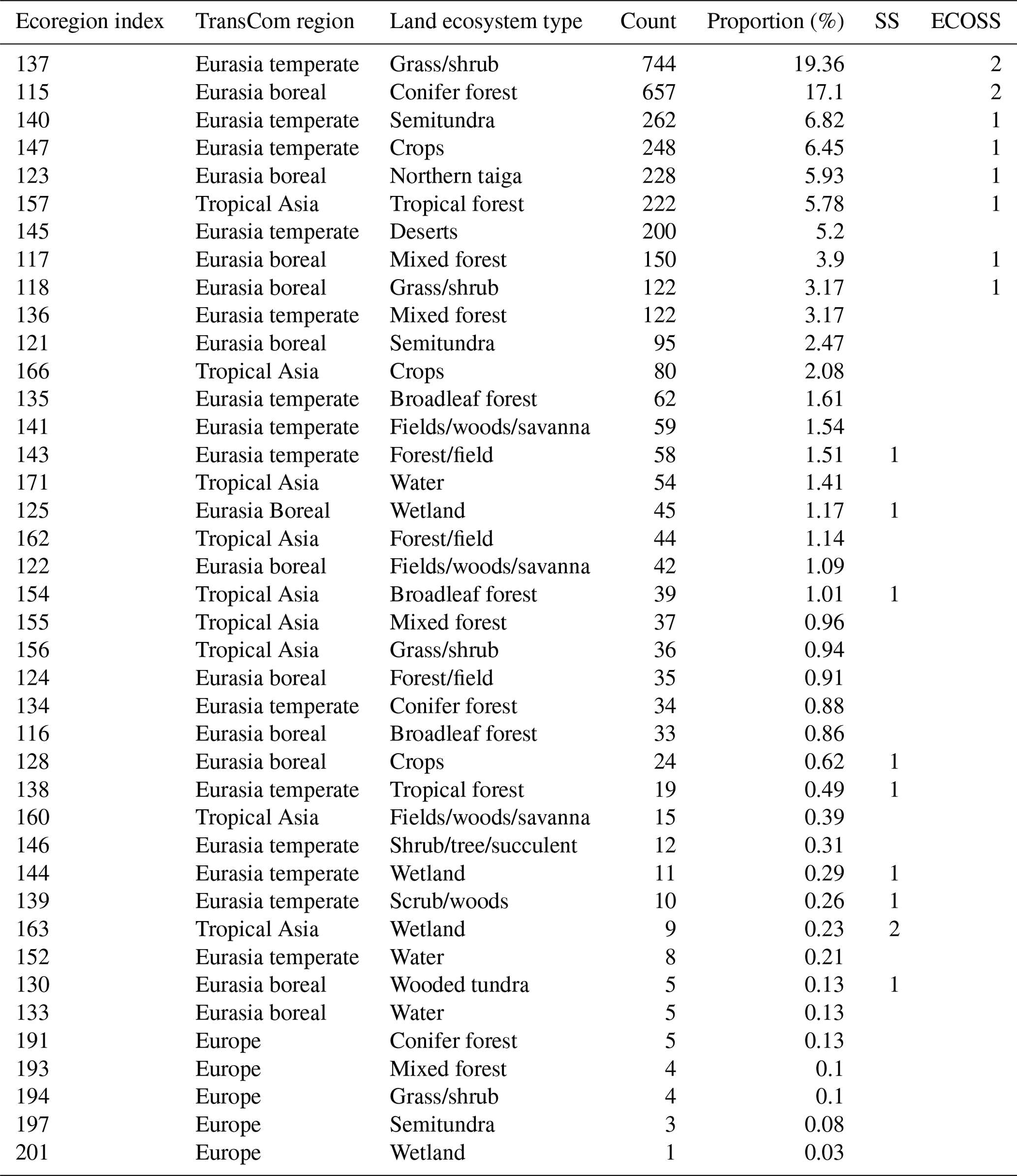
TM5 is an off-line transport model used to calculate the transport of CO2 (Krol et al., 2005), which utilizes the atmospheric fields of the ERA-Interim reanalysis data of the European Centre for Medium-Range Weather Forecasts (ECMWF). TM5 utilizes the estimated surface CO2 fluxes at each grid point based on Eq. (1) to calculate the spatiotemporal distribution of the model atmospheric CO2 concentrations. From the estimated surface CO2 fluxes at each grid point, the model atmospheric CO2 concentrations at the times and locations of the observation data are calculated, and these are used for the data assimilation process. The horizontal resolution of TM5 is globally and the nested horizontal grid is over Asia, with a verification region inside of the nested domain over Asia (Fig. 1). The number of ecoregions in the verification region is 40, of which 36 are Asian ecoregions (Fig. 1b) and 4 are ecoregions of Europe. Since the proportion of the 4 European ecoregions is approximately 0.5 % of the verification region (Table 3), the verification region was considered to be located over Asia. A two-way nested grid was used to optimize surface CO2 fluxes in Asia. The model run including both forward and inversion runs was done globally with nesting over Asia and verification was done over the verification region located in Asia. Table 1 summarizes the priori flux emissions used for the flux module and describes the TM5 setup.
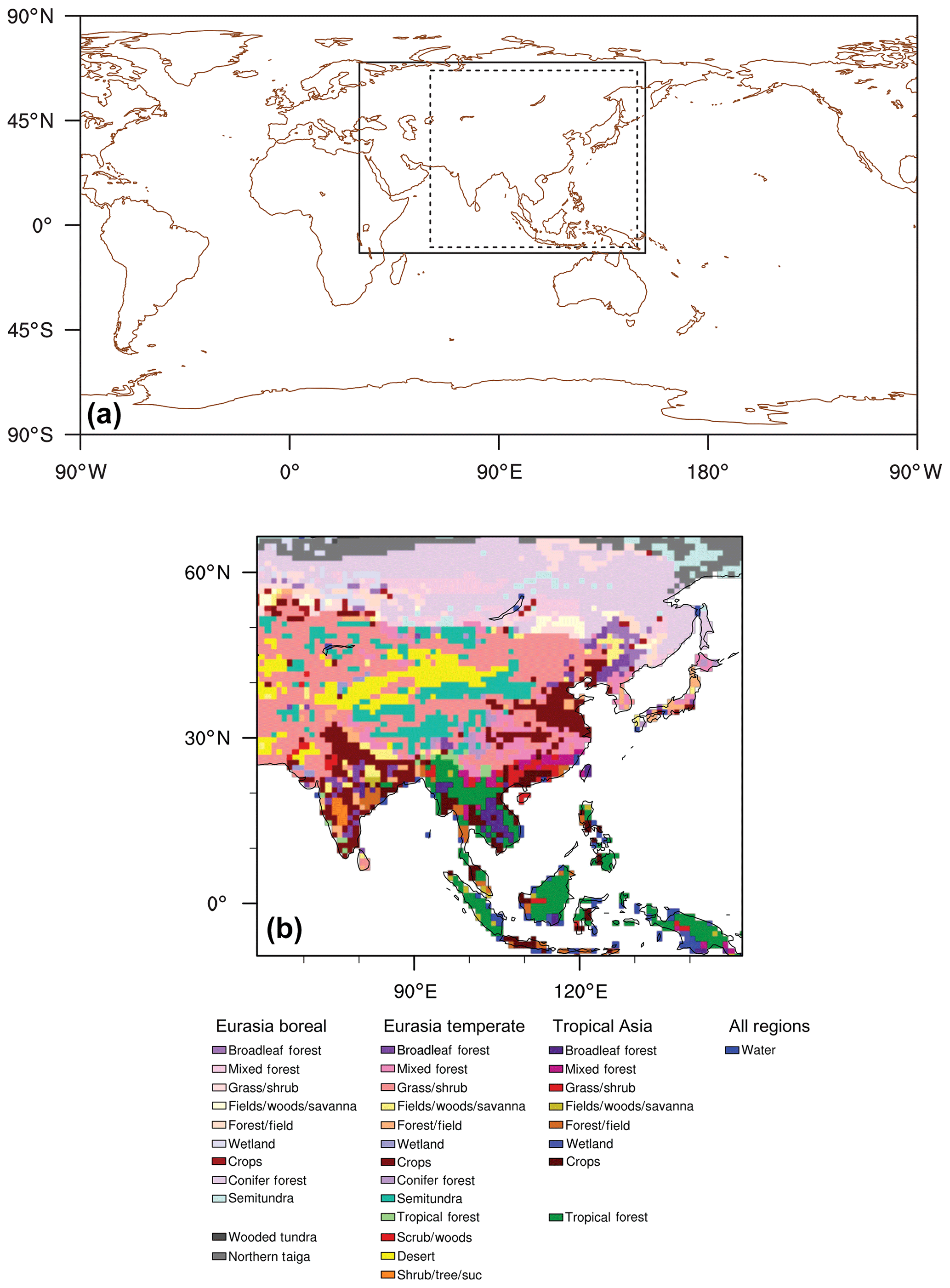
Figure 1The distribution of (a) the nested TM5 model domain over Asia (black solid rectangle) and verification domain (black dashed rectangle) and (b) ecoregions in Asia used in this study.
Table 1The model configuration and a priori fluxes used in this study.
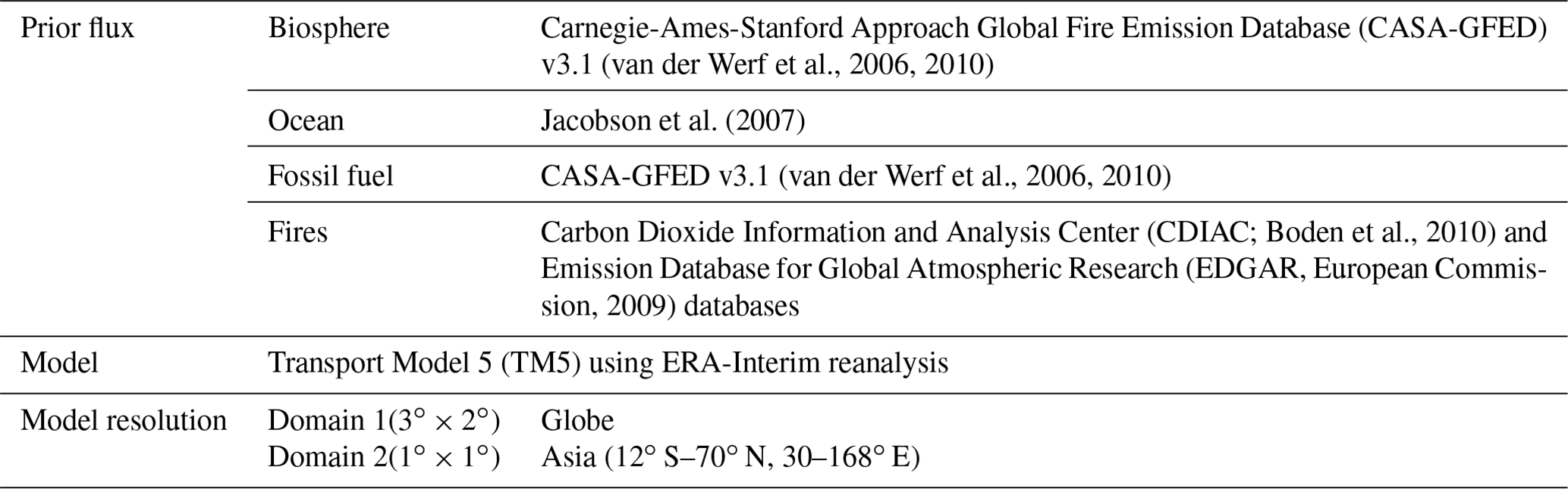
Table 2Brief description of the experiments conducted in this study.
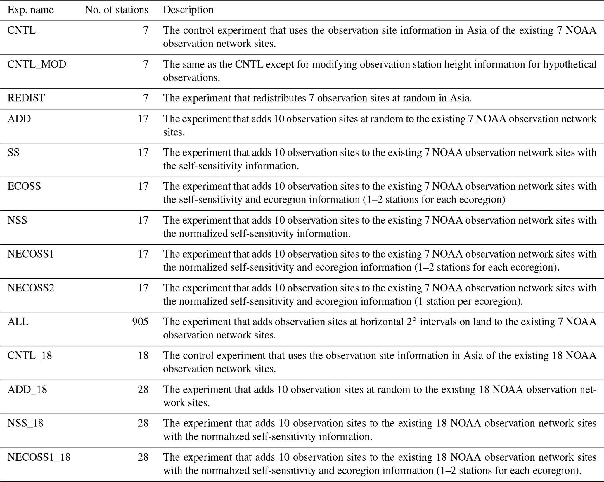
Table 3The information of the ecoregions in the verification domain (see also Fig. 1b) and the distribution of observation sites for the SS and ECOSS experiments.
An ensemble square root Kalman filter (EnSRF), one of the EnKF data assimilation methods (Evensen, 1994; Whitaker and Hamill, 2002), was employed in this study to optimize the scaling factor. EnSRF assimilates observation data one by one, and updates the analysis of ensemble mean and perturbations separately based on the following equations:
where xa and xb describe the analysis and background value of the state vector (x), and x′ are the ensemble mean and perturbation of the state vector, yo is the observation vector, and H describes the observation operator that transforms the state vector from the model space to the observation space. TM5 acts as the observation operator in CT2013B (Krol et al., 2005; Peters et al., 2005; Kim et al., 2016, 2018a). K and denote the Kalman gain matrix and the reduced Kalman gain calculated as follows:
where Pb is the background error covariance, R is the observation error covariance for each observation, and α is a scalar value that is multiplied to Kalman gain matrix at every calculation of the analysis, defined as
By calculating the ensemble mean and perturbation independently, the underestimation of the analysis error covariance could be prevented (Whitaker and Hamill, 2002; Kim et al., 2012). PbHT and HPbHT can be calculated as follows:
where m is the number of ensemble members.
Unlike the approach of NWP, the time for CO2 dispersing around the atmosphere needs to be considered for CO2 data assimilation. Accordingly, a time lag is introduced in updating the scaling factor during the data assimilation process to consider the information for analysis time as well as for pre-analysis time. A time lag of 5 weeks is employed in this study, consistent with previous studies (Peters et al., 2007, 2010; Kim et al., 2012, 2014a, b, 2017).
In the EnSRF, the covariance localization method is necessary to reduce the impact of the sampling error due to the limited size of the ensemble and to avoid filter divergence due to the underestimation of the background error covariance (Houtekamer and Mitchell, 2001). Because calculating the physical distance between scaling factors is not possible, instead of the covariance localization method, a statistical method is applied in this study. In this method, a Student's t test is applied to the correlations between the ensemble of the model CO2 concentrations and the ensemble of the scaling factors, and the Kalman gain matrix is then made to be zero for the cases where it has an insignificant statistical t value (i.e., 95 % significance level), to exclude those insignificant impacts (Peters et al., 2007).
The optimized mean scaling factor after one analysis cycle is used as one of the prior mean scaling factors for the next analysis step as follows:
where is a prior mean scaling factor for the current analysis step, and and denote posterior mean scaling factors of previous analysis cycles. The information of current analysis propagates to the next step using Eq. (9) (Peters et al., 2007).
2.2 Influence matrix
The influence matrix of the EnKF system can be calculated as described in Liu et al. (2009) and Kim et al. (2014a). The analysis of the state vector and the influence matrix (So) that shows the contribution of the observation vector (yo) to the analysis at the observation space (ya) (i.e., the projection of analysis state vector xa on the observation space or model analysis equivalent to observations at observation locations) can be defined as follows:
where In is the identity matrix (n is the size of analysis or background state vector). The influence matrix is proportional to the analysis error covariance and inversely proportional to the observation error covariance. Using Eq. (8), So is expressed as follows:
where HXa is the analysis of the ensemble perturbation at the observation space. The ith component of HXa is defined as follows:
where is the ith member of the analysis ensemble, and h(⋅) denotes the linearized or non-linearized observation operators. Following Liu et al. (2009), we assume no correlations between observation errors, and the diagonal element of this influence matrix (i.e., self-sensitivity) is calculated as follows:
where is the observation error variance for the jth observation.
According to Liu et al. (2009) and Kim et al. (2014a), So represents the sensitivity of the analysis state vector ya to the observation state vector yo in the observation space (i.e., location). So has a value between 0 and 1, which shows the contribution of a CO2 observation to the analyzed CO2 at the observation site. If So is close to 0, the analysis is mainly derived from the background. In contrast, the influence of observation data to the analysis increases as So goes to 1. The self-sensitivity was used as a criterion for selecting the observation locations in designing the observation network.
2.3 Simulated hypothetical observation and experimental setup
In this paper, simulated hypothetical observations were created and used to design the observation network. Simulated hypothetical observations with similar values and seasonal variations compared to real CO2 observations were generated by averaging model CO2 mole fractions from the experiment conducted with real NOAA observation data (EXTASI) and model CO2 mole fractions from the experiment with a fixed scaling factor of 1 (SF1). In the EXTASI experiment, the real CO2 mole fraction data were used to update the scaling factors in Eq. (1) to estimate the surface CO2 fluxes. In contrast, in the SF1 experiment, the scaling factors were fixed as 1.
Figure 2 shows the station-averaged time series of CO2 mole fractions from real observations (OBS), EXTASI, SF1, and an average (i.e., simulated hypothetical observations: TRUE, hereafter) of EXTASI and SF1. The time series of EXTASI is the closest to that of OBS, whereas that of SF1 with a static scaling factor (i.e., 1) differs from OBS, particularly in summer. Kim et al. (2017, 2018) have shown that the largest difference in surface CO2 flux estimation between experiments with different settings appears in summer, which is associated with a more sensitive response of inversion results to the inversion model configurations for the active season of the terrestrial ecosystem. The time series of TRUE is located between that of EXTASI and SF1, which implies that the difference between TRUE and OBS is smaller compared with that between SF1 and OBS. TRUE is the simulated hypothetical observation that is similar to the EXTASI assimilating real NOAA observation data, but is not the same as the EXTASI. This setup prevents EXTASI from having an advantage in the observation network experiments. If TRUE is the same as EXTASI, then assimilating TRUE data at the observation locations used in EXTASI would render the observation network used in EXTASI the optimal network in terms of several verification measures used in this study. One limitation of this choice of hypothetical data is that it uses the same spatial distribution of fluxes within an ecoregion as used in the inversion method, whereas in reality the within-region flux distribution could be different.
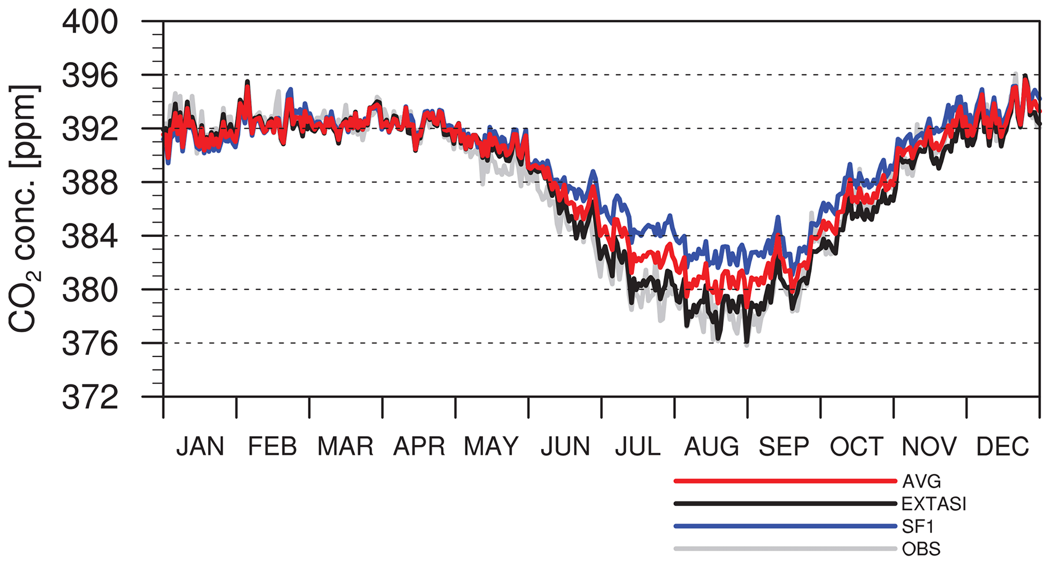
Figure 2Time series of CO2 concentration from hypothetical observations, model simulations, and real observations. The gray solid line (OBS) denotes the value of real observation data, the black solid line indicates the value from the EXTASI experiment, the blue solid line denotes the value of the SF1 experiment, and the red solid line (AVG) denotes the average of the EXTASI and SF1, which was regarded as TRUE observation data in this study.
Each hypothetical observation site has one CO2 observation per day and exists within the limited Asia domain shown in Fig. 1. The simulated values around afternoon (i.e., 13:00 local standard time, LST) in the midlatitudes in the Northern Hemisphere are averaged and utilized as TRUE data. The observation height of TRUE data at each site is set to 5 m greater than the model elevation of the grid point in order to use the observation operator for flask observation developed in NOAA. Moreover, each observation site is more than 1000 km apart from other sites, located lower than 2000 m above sea level, and located on the land regions in the TransCom Region from Gurney et al. (2002). This configuration was made to consider real-world constraints to optimize the surface CO2 fluxes in Asia. Observation error for the CO2 observations was set to 3 ppm, consistent with the previous setting of 3 ppm for continuous observation site types (Peters et al., 2007; Kim et al., 2014b, 2017).
All simulation results were produced under identical conditions except for the observation locations and data. A total of 150 ensemble members were used for data assimilation, and experiments were carried out from 27 September 2007 to 4 January 2009. The first 3 months of the experiments were considered as the spin-up period; thus the analysis was conducted from 27 December 2007 to 4 January 2009.
As the experimental results depend on the distribution of observation sites, appropriate choices of the observation network are important. Experiments are therefore configured to investigate the impact of redistributing observation sites of CT2013B (hereafter, existing observation sites or network) and that of adding extra observation sites to the existing observation network based on random, self-sensitivity, and ecoregion information. Figure 3 shows the hypothetical observation networks used in this study. Figure 3a presents the distribution of seven observation sites in Asia from the observation network of CT2013B, which are mostly located between 30 and 45∘ N. The experiment and simulation results using this observation network were denoted as CNTL. Since the CNTL could have disadvantages due to the use of real observation information (i.e., the observation height of simulated sites are always above 5 m from model topography, but this is not the case for CNTL), an additional experiment identical to CNTL, except that the observation heights were assigned above 5 m from the model topography in the same way as for hypothetical observations, was also conducted and denoted as CNTL_MOD. Figure 3b, c, and d show the distribution of three observation networks, in which the seven observation sites in Asia are randomly redistributed subject to a minimum spacing of 1000 km. To obtain general results without sampling error, each random redistribution experiment was performed three times with different sets of randomly distributed observation sites, as denoted in previous observation network studies (e.g., Yang et al., 2014). The average of three random redistribution experiments was denoted as REDIST, to check the impact of the reallocation of the existing observation network.
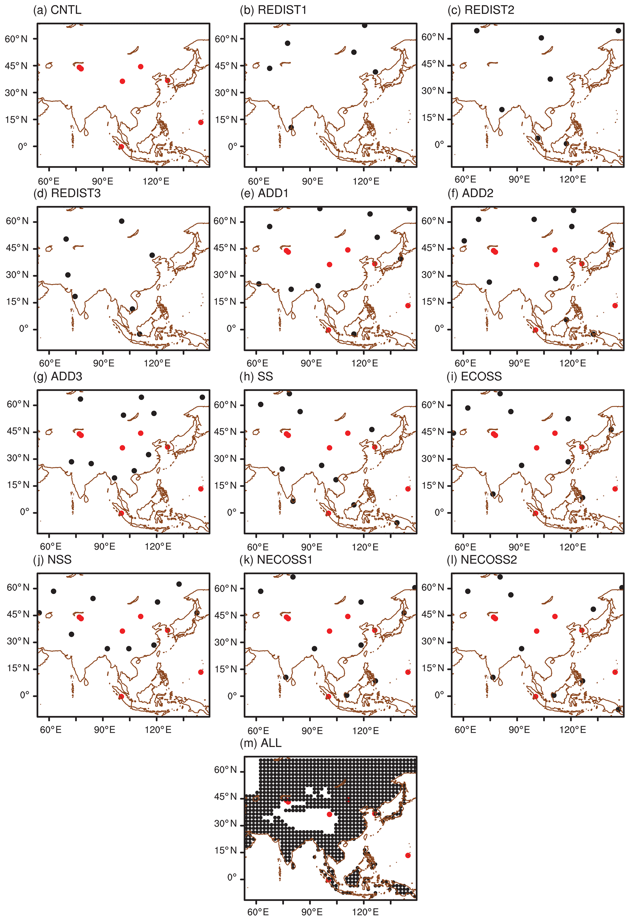
Figure 3The distribution of observation sites in each observation network: (a) the CNTL and CNTL_MOD, (b–d) the REDIST, (e–g) the ADD, (h) the SS, (i) the ECOSS, (j) the NSS, (k) the NECOSS1, (l) the NECOSS2, and (m) the ALL experiment. Red dots denote the observation sites of the NOAA observation network and black dots denote the hypothetical observation sites. Note that cases (b–l) require a minimum 1000 km spacing between sites.
Figure 3e–m suggest the distributions of the observation networks to examine the impact of adding additional observation sites to the existing observation network. Note that all additional sites are also subject to the 1000 km separation criterion. The 10 extra observation sites were added as this number seems realistically viable for the future, considering the cost of operating and maintaining CO2 observation sites. Specifically, Fig. 3e–h show the distribution of three observation networks with an additional 10 observation sites added randomly to the existing observation network. The average of these three experiments was denoted as ADD. The experiment adding 10 observation sites to the existing observation network based on self-sensitivity is denoted as the SS experiment (Fig. 3h). The experiment adding 10 observation sites to the existing observation network based on both self-sensitivity and ecoregion information is denoted as the ECOSS experiment (Fig. 3i). The ECOSS experiment was conducted as the scaling factor in CT2013B is updated based on ecoregion, thus only considering self-sensitivity makes the added observation sites cluster in a specific ecoregion and causes disadvantages in optimizing the scaling factor. As the self-sensitivity is generally inversely proportional to the number of assimilated observations (Kim et al., 2014a, 2017), the self-sensitivity normalized by the number of assimilated observations is also considered and utilized. Figure 3j–l show the distributions of the observation network for three experiments that used the normalized self-sensitivity as the selection criterion for added observation sites. The NSS experiment (Fig. 3j) used only the normalized self-sensitivity as the selection strategy. The observation sites of the NECOSS1 (Fig. 3k) and NECOSS2 (Fig. 3l) experiments were added based on the normalized self-sensitivity and ecoregion information. The NECOSS1 experiment allocated one or two observation sites per ecoregion, whereas NECOSS2 allocated one observation site per ecoregion. In addition, the observation networks that have observation sites at every 2∘ interval on the land (Fig. 3m, ALL experiment) are suggested as the reference to examine the maximum possible impact of additional observation sites. In the ALL experiment, the observation locations that are located 2000 m above the mean sea level over the Tibetan Plateau are not included due to their difficult accessibility and maintenance as practical observing sites.
The normalized self-sensitivity for the jth observation is defined as follows:
where NALL denotes the total count of observation sites of the ALL experiment, and Nj is the number of observation sites that have the same ecoregion as the jth observation site in the ALL experiment. Thus, normalized self-sensitivities were calculated by multiplying self-sensitivities by the ratio of the number of observation sites in a specific ecoregion to that in the ALL experiment.
The effect of the redistribution of the existing observation network and adding additional observation sites on the existing observation network can be diagnosed through the experiments detailed above. The method of adding observation sites in the experiments using self-sensitivity and ecoregion information is described in more detail in Sect. 3. Table 2 describes the list of observation network experiments and their relevant information.
2.4 Verification method
The nested model domain over Asia and the verification area (−9.5∘ S–66.5∘ N, 60.5–149.5∘ E) are shown in Fig. 1. The optimized surface CO2 flux in each experiment was verified against the hypothetical surface CO2 fluxes corresponding to TRUE. Weekly surface CO2 fluxes were analyzed to evaluate the performance of observation network experiments because the scaling factor has a weekly resolution. The Pearson product-moment correlation coefficient (pattern correlation, PC) and the root mean square difference (RMSD) were compared and calculated as follows:
where EXPi and TRUEi are the surface CO2 fluxes at the ith model grid point of an experiment and TRUE, respectively, and n is the total number of model grid points in the verification domain shown in Fig. 1.
To investigate the reduction of uncertainties for each experiment after data assimilation, uncertainty reduction (UR; Peters et al., 2005; Meirink et al., 2008; Chevallier et al., 2009b; Feng et al., 2009; Kim et al., 2014a, 2017, 2018b) was calculated as:
where σCNTL and σEXP denote 1σ standard deviations of the optimized scaling factor for the CNTL and an experiment. The UR was used to check the improvement of observation network experiments by comparing the posterior uncertainties of experiments with those of CNTL (i.e., the reference experiment).
3.1 Effect of an observation network with observation sites redistributed randomly
Figure 4 shows the time series of the 3-week moving average of RMSD for surface CO2 fluxes from the CNTL, CNTL_MOD, and REDIST experiments. The RMSDs of all three experiments are larger in summer, which may be caused by the larger surface CO2 fluxes in this season as seen in the strong drawdown of CO2 mole fractions shown in Fig. 2. The time series of RMSDs of CNTL and CNTL_MOD have similar variations except for a slight phase shift, whereas that of REDIST shows a comparatively smaller increase in the RMSD in the summer. Specifically, the maximum RMSD of CNTL is 201 in mid-July and that of CNTL_MOD is 192 early in July, but that of REDIST is 127 at the beginning of June. In addition, the maximum and minimum RMSDs of three redistribution experiments are mostly smaller than the RMSDs of CNTL and CNTL_MOD. Thus, REDIST is better than CNTL in simulating surface CO2 fluxes in Asia in summer.
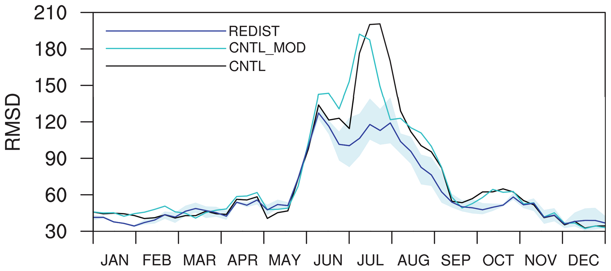
Figure 4Time series of the 3-week moving average of RMSD of surface CO2 flux (gC m−2 yr−1) for the CNTL (black solid line), CNTL_MOD (cyan solid line), and REDIST (blue solid line) experiments. The blue shaded band denotes the minimum and maximum RMSD across three random redistribution experiments.
REDIST clearly outperforms CNTL and CNTL_MOD in summer, and an overall improvement is also observed from the comparison of the three experiments. This implies that merely redistributing current observation sites in Asia could have more benefits in optimizing surface CO2 fluxes. This result seems to be somewhat attributable to the fact that most observation sites in Asia in the NOAA observation network of CT2013B are located in midlatitudes (∼35–45∘ N).
Furthermore, CNTL and CNTL_MOD are not much different in simulating surface CO2 fluxes, which implies that the selection strategy of observation height in making hypothetical observations does not greatly affect the evaluation of the various observation networks. The real height information of the NOAA observation network in CNTL is therefore used for existing observation sites in Asia, and the observation height of additional hypothetical sites is set to 5 m above the model topography in the following experiments.
3.2 Effect of an observation network with extra observation sites added randomly
Figure 5 presents the time series of the 3-week moving average of RMSD for surface CO2 fluxes from the CNTL, ADD, and ALL experiments, which clearly show the effect of randomly added observation sites. The three experiments show larger RMSD values in the summer compared to other seasons, which is similar to the previous random redistribution experiments in Sect. 3.1. The RMSDs of ADD and ALL with more observation sites generally remain low during the simulation period. Except in summer, the time series of RMSD of ADD is similar to or slightly lower than that of CNTL. In summer, the maximum RMSD of ADD is reduced to 109, maintaining lower values during the summer and not showing any sudden increase. In addition, the maximum and minimum RMSDs of three addition experiments are mostly smaller than the RMSD of CNTL. ALL has the minimum RMSD among the three experiments throughout the simulation period and reaches a maximum of only 34 in early July. Since this number does not exceed the minimums of CNTL and ADD, the ALL experiment can be regarded as the best observation network. This suggests that an accurate and stable optimization of surface CO2 fluxes in Asia is possible if CO2 observation sites are sufficient.
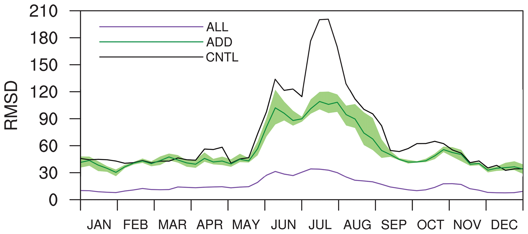
Figure 5The same as Fig. 4 except for the CNTL (black solid line), ADD (dark green solid line), and ALL (purple solid line) experiments. The green shaded band denotes the minimum and maximum RMSD across three random addition experiments.
The result of the observation network experiments with randomly added extra observation sites (i.e., ADD) also implies that the seven observation sites in Asia described in CT2013B do not seem to be sufficient to fully optimize the surface CO2 fluxes in the region. Although the ADD experiment with 10 randomly added extra observation sites shows an improvement in optimization, more observation sites are necessary for optimizing surface CO2 fluxes in Asia, considering the result of the ALL experiment. Moreover, the simulation result of the ADD experiment does not much outperform that of the REDIST experiment, although more observations were used. This implies that further consideration is required when adding observation sites to the existing observation network. Thus, rather than just adding observation sites randomly, selecting and adding more influential observation sites for Asia is crucial to construct an efficient surface CO2 observation network.
3.3 Effect of an observation network with extra observation sites added using self-sensitivity and ecoregion information
Considering the simulation results of Sect. 3.2, the addition of extra observation sites to the existing observation sites could improve the performance in simulating surface CO2 fluxes in Asia. In particular, the ALL experiment, which added many observation sites under the given modeling framework, shows a high level of reproducibility of TRUE. However, adding more than 900 observation sites in Asia does not seem to be possible in real situations. Moreover, the expected effect from the extra observation sites may not be effective if the additional observations are not influential. Thus, the efficient selection and supplementation of observation sites is inevitable considering these constraints under realistic conditions.
In this study, self-sensitivity information obtained from the ALL experiment and ecoregion information used in CT2013B were used as additional strategies for the purpose of adding possible efficient observation sites in Asia. Since the self-sensitivity is the metric showing the impact of observations at each observation site for the model simulation results, as stated in Sect. 2.2, it can be used as a strategy for selecting potential observation sites. In addition, the proportion of each ecoregion in the Asia domain can also be utilized as a strategy in choosing observation sites, as the calculation of surface CO2 fluxes is based on the scaling factor for each ecoregion in CT2013B, and the scaling factor updated in the data assimilation process has the possibility to be more affected by the observation sites located in the same ecoregion (CarbonTracker Documentation CT2013B Release, 2015).
Figure 6 shows the spatial distribution of self-sensitivity from the ALL experiment. Although the self-sensitivity of each observation site varies from the others, four influential regions with high sensitivities are located in western Siberia, the southern part of the Tibetan Plateau, and southeastern and northeastern Asia. The highest (lowest) self-sensitivity of the hypothetical observation sites is 4.02 % (0.04 %). Thus, the likelihood of using observations located in the aforementioned four regions increases when considering the self-sensitivity as the selection strategy. In contrast, the observation sites located in southwestern Asia and eastern Siberia are rarely chosen for the optimization due to the low value of self-sensitivity.

Figure 6The spatial distribution of self-sensitivities (%) during the experimental period obtained from the ALL experiment.
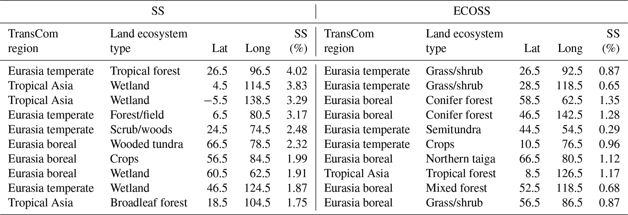
The self-sensitivity used for the SS and ECOSS experiments is the pure self-sensitivity without considering the number of assimilated observations. The 10 observation sites of the SS experiment were selected by employing self-sensitivity from the numerical order (highest first) and following the addition criteria (i.e., 1000 km distance between sites and observation height 5 m above the model topography) used in Sect. 2.3. For the ECOSS experiment, the proportions of ecoregions in the Asia verification domain were calculated from the model grid points. Following this, the observation sites were selected from the order of principal ecoregions with self-sensitivity information. Specifically, the land ecoregion information, omitting that of the oceans and deserts, was utilized for the selection criteria as the land in the Northern Hemisphere is crucial for the global carbon exchange. Table 3 displays the proportions of ecoregions in the Asia verification domain and the distribution of observation sites in SS and ECOSS. As the ecoregions with 115 (conifer forest, Eurasia boreal) and 137 (grass/shrub, Eurasia temperate) indices constitute relatively large proportions of the ecoregions in Asia (Table 3), two observation sites were assigned for each of these two ecoregions. The other ecoregions have one observation site per ecoregion. When selecting the aforementioned two and one observation sites in the ecoregions, the observation sites with the highest self-sensitivities were selected. The observation sites of SS are mostly located in ecoregions that constitute lower proportions compared to those of ECOSS because the self-sensitivity is generally inversely proportional to the number of assimilated observations, as shown in Kim et al. (2014a, 2017). Selected sites are listed in Table 4.
Table 4The locations and self-sensitivities for the observation sites in the SS and ECOSS experiments.
The time series of the 3-week moving average of RMSD of the simulated surface CO2 fluxes for the ADD, SS, and ECOSS experiments are shown in Fig. 7, which shows the impact of additional observation sites considering self-sensitivity information. The ECOSS experiment that considered both self-sensitivity and ecoregion information maintains lower RMSD than the ADD experiment over the experimental period. In addition, the maximum and minimum RMSDs of three addition experiments are mostly larger than the RMSD of ECOSS. Compared to ADD and CNTL, the SS experiment demonstrates slight improvement in the other seasons except summer, whereas the ECOSS experiment demonstrates improvement over the whole experimental period. To confirm that the improvement is not just from including the ecoregion information, an additional test was performed using the same regions as ECOSS and the locations of lowest self-sensitivity in those regions. The resulting RMSD is similar to ADD and SS, confirming that both high self-sensitivity and ecoregion information are needed to give the improved results of ECOSS compared to randomly added observation sites.

Figure 7The same as Fig. 4 except for the ADD (dark green solid line), SS (yellow solid line), and ECOSS (red solid line) experiments. The green shaded band denotes the minimum and maximum RMSD across three random addition experiments.
The increased RMSD of SS during the spring–summer period compared to that of ADD seems to be related to the DA method used in CT2013B. As most observation sites added in SS are located in the ecoregions with relatively small proportions of the Asia domain (Table 3), they may have disadvantages in optimizing the scaling factor of major ecoregions. This is somewhat relevant to the distribution of observation sites in the ALL experiment, which has observation sites at 2∘ intervals, consequently leading to the uneven distribution of observation sites (i.e., major ecoregions with more observation sites and minor ecoregions with fewer observation sites) in Asia. As the self-sensitivity generally has an inverse relationship with the number of assimilated observations, the self-sensitivities of major ecoregions are typically lower than those of minor ecoregions, as shown in Table 4.
The simulation results of SS and ECOSS confirm that influential observation sites for optimizing surface CO2 fluxes in Asia certainly exist, and the self-sensitivity information could be used for designing the observation network. The ECOSS experiment especially, which considers both self-sensitivity and ecoregion information, shows a better performance compared to the SS experiment, which suggests that considering characteristics of the specific model and data assimilation configurations can also contribute to the improvement in optimization. This further implies that an observation network based on the self-sensitivity and ecoregion information could be better for optimizing surface CO2 fluxes in Asia than that based on randomly added observation sites, though the same number of observations are used.
3.4 Effect of an observation network with extra observation sites added using normalized self-sensitivity and ecoregion information
As stated in Sect. 3.3, using the pure self-sensitivities acquired from the ALL experiment for observation network studies could be inappropriate in certain situations because they were derived from an uneven number of sites for each ecoregion. Thus, self-sensitivity could be normalized (Eq. 15) and used for the selection of observation sites. Table 5 shows the information for observation sites in the NSS, NECOSS1, and NECOSS2 experiments that used the normalized self-sensitivities as the selection strategy. The observation sites of the NSS experiment are located only in the 115 (conifer forest) and 137 (grass/shrub) ecoregions. This is because they have higher normalized sensitivities than other regions as they constitute large proportions of the ecoregions of Asia, as shown in Table 3. Additionally, the NECOSS1 and NECOSS2 experiments were conducted to examine the impact of additional observation sites depending on the choice of ecoregion. For the NECOSS1 experiment, two observation sites were added to the 115 (conifer forest) and 137 (grass/shrub) ecoregions and one observation site each was allocated to the other 6 ecoregions. In contrast, the NECOSS2 experiment allotted one observation site to each ecoregion. The observation sites in NECOSS1 and NECOSS2 in the ecoregions were selected by the order of highest normalized sensitivities in each ecoregion. Note that the 1000 km site separation criterion is still applied.
Table 5The locations and ecoregion indices for the observation sites in the NSS, NECOSS1, and NECOSS2 experiments.
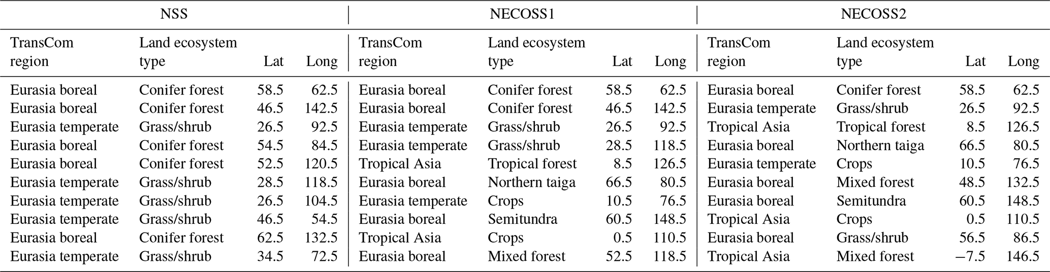
Figure 8 shows the time series of the 3-week moving average of RMSD of the simulated surface CO2 fluxes for the ADD, NSS, NECOSS1, and NECOSS2 experiments, which shows the impact of using normalized self-sensitivities for the selection of additional observation sites. The NSS, NECOSS1, and NECOSS2 experiments show lower RMSDs compared to the ADD experiment. The RMSD of NSS is lower than that of ADD for most of the time, which is different from SS that showed a degradation in summer and little improvement in other seasons compared to ADD in Fig. 7. Moreover, the NECOSS1 and NECOSS2 experiments that additionally considered the ecoregion information demonstrate a further reduction in RMSD, especially in summer. The NECOSS1 and NECOSS2 experiments have a slightly lower RMSD than ECOSS that considered pure self-sensitivities and ecoregion information. The NECOSS1 and NECOSS2 experiments do not show significant differences since the two networks are quite similar.
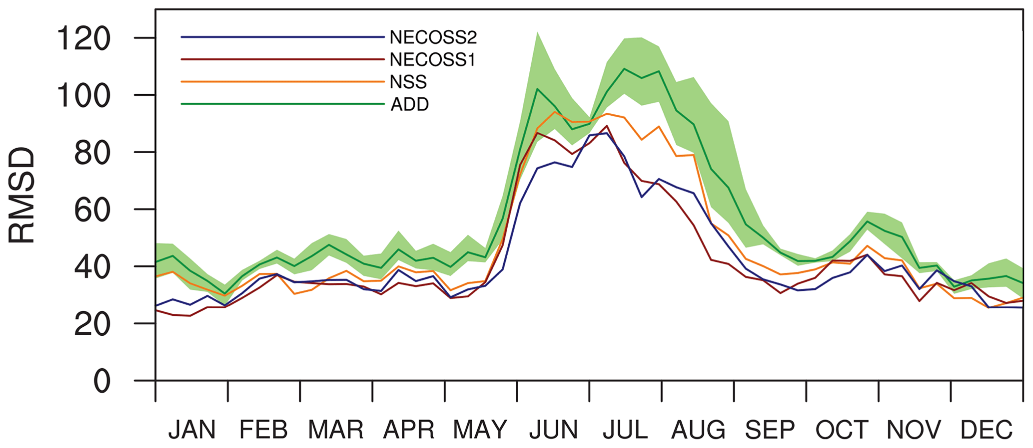
Figure 8The same as Fig. 4 except for the ADD (dark green solid line), NSS (dark orange solid line), NECOSS1 (dark red solid line), and NECOSS2 (navy blue solid line) experiments. The green shaded band denotes the minimum and maximum RMSD across three random addition experiments.
The simulation results using the normalized self-sensitivities reconfirm that the self-sensitivity information could be used in designing the observation network. By considering the DA method of CT2013B that optimizes scaling factors assigned in ecoregions, the experiments using normalized self-sensitivities could make simulations better than those using pure self-sensitivity. In addition, the additional consideration of ecoregion in the experiments using normalized self-sensitivities also contributes to improvements, which implies that the model's characteristics, such as ecoregion information, could also be one of the factors to be used in designing the surface CO2 observation network.
3.5 Horizontal distributions of RMSD and uncertainty reduction
Figure 9 shows the spatial distribution of the average of weekly RMSD calculated from the surface CO2 fluxes in Asia for the whole year; the distribution for summer is similar. The CNTL shows the highest RMSD among the experiments, with peaks mainly located in the Siberian area (Fig. 9a). The REDIST experiment shows a decrease in the high RMSD of the Siberian area shown in CNTL, but the RMSDs of eastern China and the southeastern part of the Tibetan Plateau (the Indochina Peninsula) increase slightly, and the RMSDs of northern India and the northeastern part of Asia remain nearly unchanged compared to CNTL (Fig. 9b). The distribution of RMSD in the ADD experiment is fairly similar to that of REDIST, except for the decrease in the RMSD near the Tibetan Plateau and in southeastern Asia (Fig. 9c). Such a spatial distribution of RMSD in the ADD experiment implies the need for supplementing observation sites efficiently. Figure 9d clearly shows the reduction in the RMSD of northern India and the southeastern region of the Tibetan Plateau in the SS experiment compared to the REDIST and ADD experiments. This proves the impact of considering self-sensitivity information for observation network studies. However, the performance of the SS experiment on some Siberian inland areas is poorer than those of the REDIST and ADD experiments, due to the relative absence of observation sites for that region. The ECOSS experiment using the ecoregion information shows comparatively lower RMSD in the Asia domain, except for the southeastern part of the Tibetan Plateau and northeastern Asia (Fig. 9e). The RMSD distribution of the NSS experiment confirms that the RMSD of the Siberian area is much reduced compared to that of the SS experiment, though its overall pattern is similar (Fig. 9f). The RMSDs of the NECOSS1 and NECOSS2 experiments are analogous to that of the ECOSS experiment (Fig. 9g). This can be attributed to the fact that most observation sites in those three experiments are identical (Tables 4 and 5). The simulated RMSD of the ALL experiment is the lowest in most of the domain among all sensitivity experiments (Fig. 9i). Such simulation results reconfirm that the observation network in Asia needs to be organized in a more efficient way to gain better optimization results of surface CO2 fluxes.
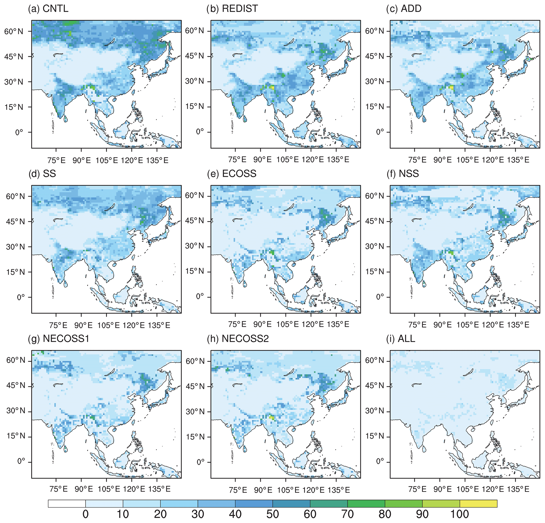
Figure 9The spatial distribution of the average of weekly RMSD of surface CO2 fluxes (gC m−2 yr−1) for (a) the CNTL, (b) the REDIST, (c) the ADD, (d) the SS, (e) the ECOSS, (f) the NSS, (g) the NECOSS1, (h) the NECOSS2, and (i) the ALL experiments.
Figure 10 shows the UR derived from the experiments, which corresponds with the previous results. Compared to the CNTL experiment, the uncertainty of the REDIST experiment is much reduced in the Siberian area, but the impact of REDIST is low south of 50∘ N (Fig. 10a). Such a result seems to be related with the high UR values in the Siberian region in CNTL, because most observation sites in CNTL are located from 30 to 45∘ N. The ADD experiment with randomly added sites demonstrates slightly more UR for the inland Siberian area and the nearby areas of the Tibetan Plateau, including China and India, than REDIST (Fig. 10b). However, the UR in the Asian midlatitudes is still lower than that in other Asian regions. Although the SS and ECOSS experiments have the same number of observation sites compared with the ADD experiment, the overall UR in the Asia domain in SS and ECOSS is higher than that of ADD (Fig. 10b, c, and d). The uncertainty in the SS experiment, which has comparatively more observation sites in India and southeastern Asia, is clearly reduced for that area. In contrast, the ECOSS experiment retaining comparatively more observation sites in the inland areas of Asia shows higher UR in the land areas, although UR in India and southeastern Asia is lower than that in the SS experiment. The experiments using normalized self-sensitivities generally show distinct uncertainty reductions in inland Asia, although the UR of India and southeastern Asia in NSS is slightly lower than that of SS (Fig. 10e). This is because the observation sites of NSS are located only in the 115 (conifer forest) and 137 (grass/shrub) ecoregions. Although the UR distributions of the NECOSS1 and NECOSS2 experiments are generally similar to those of the ECOSS experiment, the uncertainties in India and southeastern Asia decrease further in NECOSS1 and NECOSS2 (Fig. 10f and g). The UR of the ALL experiment increases compared to those of other experiments as a number of observation sites in ALL sufficiently cover the Asian domain (Fig. 10h).

Figure 10The spatial distribution of uncertainty reduction (%) for (a) the REDIST, (b) the ADD, (c) the SS, (d) the ECOSS, (e) the NSS, (f) the NECOSS1, (g) the NECOSS2, and (h) the ALL experiment, against the CNTL experiment.
Table 6 summarizes the overall scores of the simulations conducted in this study. The PC is generally high due to the hypothetical observations associated with the flux distributions within ecoregions. The CNTL (ALL) experiment shows the lowest (highest) PC among the simulations. The PC of other experiments range between these. In contrast, the CNTL (ALL) experiment shows the high (lowest) RMSD among the simulations. The statistics shown in Table 6 reconfirm the impacts of redistributing current observation sites and adding extra observation sites discussed in this study. Firstly, the height specification for hypothetical observations does not seem to be very influential for the results of OSSEs as only small differences were observed between the results of CNTL and CNTL_MOD. The impact of redistribution is noticeable because the performance of the REDIST experiment was generally better than that of the CNTL experiment. Moreover, the comparison between ADD, SS, and ECOSS reaffirms that adding more observation sites to the existing sites is effective in optimizing surface CO2 fluxes, and the addition strategy needs to be more effective to have better optimization results for surface CO2 fluxes. Moreover, the NSS, NECOSS1, and NECOSS2 experiments that used both normalized self-sensitivities and ecoregion information show that the normalized self-sensitivity and configuration of the data assimilation and model can be utilized as appropriate strategies in designing an observation network that enhances simulation results. The simulation result of the ALL experiment seems to suggest a possible limit of the improvement when using the DA method in CT2013B.
Table 6The averaged statistics of surface CO2 fluxes (gC m−2 yr−1) for the experiments conducted in this study.

3.6 Additional experiments with more surface observation sites
Until now, the seven observation sites in Asia from the observation network of CT2013B were used to evaluate several strategies to determine an effective observation network for optimizing surface CO2 fluxes in Asia. Currently, surface CO2 mole fraction observations from 18 observation sites are used for CT2017 (Fig. 11). In this section, the experimental results based on 18 observation sites similar to those based on seven observation sites above are shown to reaffirm the validity of the normalized self-sensitivity and ecoregion information as selection strategies for potential observation sites. Descriptions of additional experiments are shown in Table 2. Instead of CNTL, ADD, NSS, and NECOSS1 based on seven sites, CNTL_18, ADD_18, NSS_18, and NECOSS1_18 are configured.
Figure 12 shows the time series of the 3-week moving average of RMSD of the simulated surface CO2 fluxes for the ALL, CNTL_18, ADD_18, NSS_18, and NECOSS1_18 experiments, which shows the impact of using normalized self-sensitivities for the selection of additional observation sites. CNTL_18 with 11 more sites shows a better performance when compared to CNTL shown in Fig. 4, and other experiments with 10 more observation sites compared to CNTL_18 show more improved results. The experiments with 10 more observation sites are located between the ALL and CNTL_18, and NECOSS1_18 shows the lower RMSD (37.889) compared with the RMSD of ADD_18 (39.368) and the RMSD of NSS_18 (39.133). The impact of using normalized self-sensitivities and ecoregions in determining observation sites is still shown in the additional experiments based on 18 observation sites, although the improvement is slightly reduced compared to the experiments based on 7 observation sites. The lower improvement in the experiments based on 18 observation sites compared to those based on 7 observation sites seems to be associated with the locations of 11 additional observation sites, mostly in Siberian regions, where there is a lack of observation data in CNTL, and for which there high sensitivities in Fig. 6 and high RMSD in Fig. 9a can be seen.
In this study, observation system simulation experiments using hypothetical observations were conducted to investigate the potential for an effective observation network for optimizing surface CO2 fluxes in Asia. Several experiments, including redistributing existing stations and adding observation stations to the existing observation network, were conducted to assess the performance of the current observation network and the impact of additional observation sites. For the addition experiment, random addition and addition strategies based on self-sensitivities, normalized self-sensitivities, and ecoregion information were tested and compared. The performance of each observation network was evaluated from statistics calculated from simulated surface CO2 fluxes and the uncertainty reduction.
The results indicate that further optimization of the surface CO2 fluxes in Asia could be made by redistributing existing observation sites, given that the RMSD of the redistributed experiment was reduced by 12.8 % compared to the experiment using the existing observation network (i.e., CNTL). The RMSD of the random addition experiment was reduced by 21.9 % compared to CNTL. Although the experiment based on only self-sensitivity information was not better than that based on randomly added observation sites, the experiment based on both self-sensitivity and ecoregion information reduced the RMSD by 35.2 % compared to that of CNTL. Moreover, the experiment based on both normalized self-sensitivity and ecoregion information further reduced the RMSD by approximately 40 % compared to that of CNTL. Thus, the normalized self-sensitivity and ecoregion information could be used as strategies to select observation sites to construct the surface CO2 observation network. The additional experiments based on 18 observation sites used for CT2017 also show similar results compared to the experiments based on 7 observation sites used for CT2013B, which reaffirms the validity of the normalized self-sensitivity and ecoregion information as selection strategies for potential observation sites.
Although the simulation results showed an improvement in performance, the results also suggested that adding 10 extra observation sites in Asia may not be sufficient to fully optimize surface CO2 fluxes, and more observation sites are required. Reliable observation data from some satellite sensors could supplement the model simulations on the basis of continuous surface observation sites. As the quality of satellite observation data increases, the observation network design for both surface and satellite observation data using the strategies (i.e., normalized self-sensitivity and ecoregion information) of this study will be investigated in the future.
The normalized self-sensitivity combined with the ecoregion information was useful in designing observation network in CarbonTracker. Although the ecoregion information may not be effective in other inversion systems that do not invert surface CO2 flux based on ecoregion, several strategies need to be considered and combined to get the best results in observation network design, depending on the characteristics of the platform (or system) used in designing observation network. The self-sensitivity could be used alone or adjusting to inversion systems used. Nevertheless, to evaluate the impact of ecoregion information on the results of this study, the observation network design using another inversion system (possibly without using the same ecoregion as CarbonTracker) as well as using hypothetical observations from another inversion system needs to be addressed in the future.
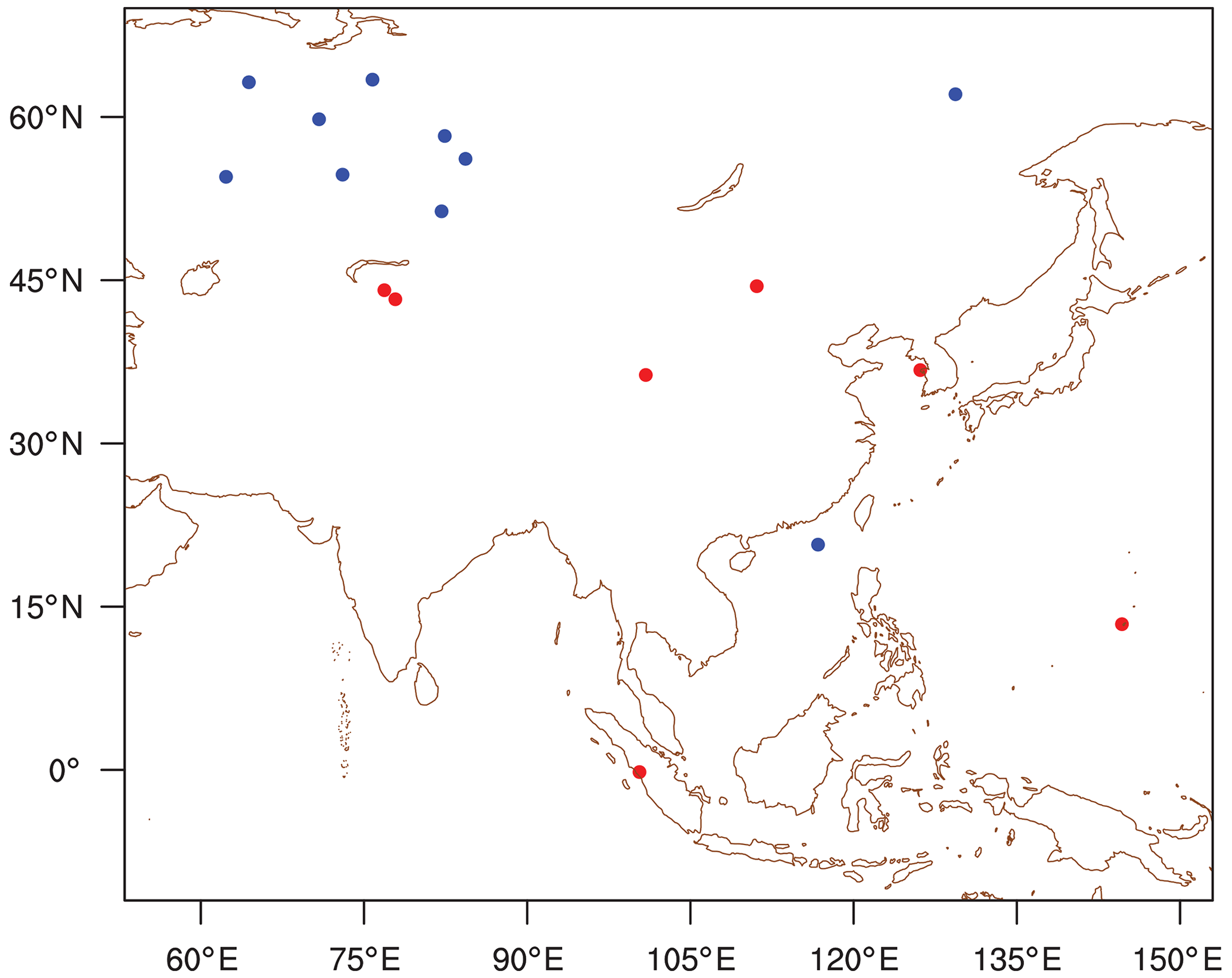
Figure 11The distribution of observation sites of CNTL_18 in Asia domain: red dots denote 7 observation sites of CT2013B and blue dots denote additional 11 observation sites of CT2017.
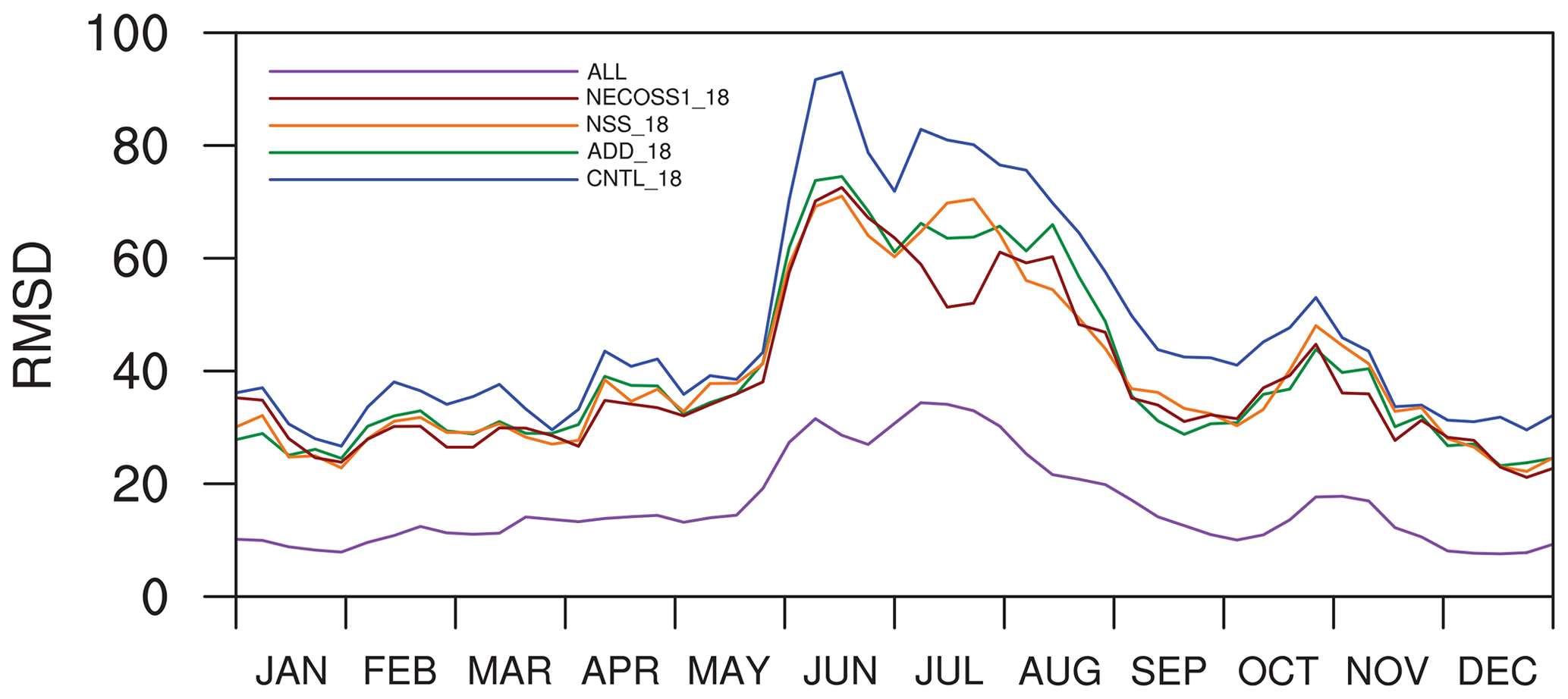
Figure 12The same as Fig. 4 except for the CNTL_18 (blue solid line), ADD_18 (dark green solid line), NSS_18 (dark orange solid line), NECOSS1_18 (dark red solid line), and ALL (purple solid line) experiments.
This study suggests a method to design and evaluate the observation network to optimize surface CO2 fluxes at the continental scale without a myriad of simulations (iterations) of the genetic algorithm or the incremental optimization used in previous studies. Thus, this approach could constitute a practical method to conduct such simulations with relatively limited computer resources. The observation network design method in this study could also be used to design an observation network to optimize global surface CO2 fluxes.
CarbonTracker data are available at the NOAA CarbonTracker home page: http://carbontracker.noaa.gov/ (last access: 20 April 2020; NOAA, 2020b). Observation data distributed by NOAA ESRL are available at the obspack home page: https://doi.org/10.3334/OBSPACK/1001 (NOAA, 2020a). The experimental results are available upon request to the corresponding author.
HMK proposed the main scientific ideas and JP contributed the supplementary ideas during the process. JP ran the observation system simulation experiments using CarbonTracker. JP and HMK analyzed the simulation results and completed the article.
The authors declare that they have no conflict of interest.
This article is part of the special issue “The 10th International Carbon Dioxide Conference (ICDC10) and the 19th WMO/IAEA Meeting on Carbon Dioxide, other Greenhouse Gases and Related Measurement Techniques (GGMT-2017) (AMT/ACP/BG/CP/ESD inter-journal SI)”. It is a result of the 10th International Carbon Dioxide Conference, Interlaken, Switzerland, 21–25 August 2017.
The authors appreciate the editor and two reviewers for their valuable comments. The authors are grateful to Andrew R. Jacobson (ESRL, NOAA, USA) for providing resources to run CarbonTracker.
This research has been supported by the Korea Meteorological Administration Research and Development Program (grant no. KMI2018-03712) and a National Research Foundation of Korea (NRF) grant funded by the South Korean government (Ministry of Science and ICT) (grant no. NRF-2017R1E1A1A303070968).
This paper was edited by Rachel Law and reviewed by two anonymous referees.
Boden, T., Marland, G., and Andres, R.: Global, regional, and national fossil-fuel CO2 emissions, Carbon Dioxide Information Analysis Center, Oak Ridge National Laboratory, US Department of Energy, Oak Ridge, TN, USA, 10, https://doi.org/10.3334/CDIAC/00001_V2010, 2010.
Byrne, B., Jones, D. B. A., Strong, K., Zeng, Z. C., Deng, F., and Liu, J.: Sensitivity of CO2 surface flux constraints to observational coverage, J. Geophys. Res.-Atmos., 122, 6672–6694, https://doi.org/10.1002/2016JD026164, 2017.
CarbonTracker Documentation CT2013B Release, CarbonTracker Team, available at: https://www.esrl.noaa.gov/gmd/ccgg/carbontracker/CT2013B/CT2013B_doc.php (last access: January 2019), 2015.
Cardinali, C., Pezzulli, S., and Andersson, E.: Influence-matrix diagnostic of a data assimilation system, Q. J. Roy. Meteorol. Soc., 130, 2767–2786, https://doi.org/10.1256/qj.03.205, 2004.
Cheng, S., Zhou, L., Tans, P. P., An, X., and Liu, Y.: Comparison of atmospheric CO2 mole fractions and source–sink characteristics at four WMO/GAW stations in China, Atmos. Environ., 180, 216–225, https://doi.org/10.1016/j.atmosenv.2018.03.010, 2018.
Cheng, Y. L., Aa, X. Q., Yun, F. H., Zhou, L. X., Liu, L. X., Fang, S. X., and Xu, L.: Simulation of CO2 variations at Chinese background atmospheric monitoring stations between 2000 and 2009: Applying a CarbonTracker model, Chinese Sci. Bull., 58, 3986–3993, https://doi.org/10.1007/s11434-013-5895-y, 2013.
Chevallier, F., Engelen, R. J., Carouge, C., Conway, T. J., Peylin, P., Pickett-Heaps, C., Ramonet, M., Rayner, P. J., and Xueref-Remy, I.: AIRS-based versus flask-based estimation of carbon surface fluxes, J. Geophys. Res.-Atmos., 114, 1–9, https://doi.org/10.1029/2009JD012311, 2009a.
Chevallier, F., Maksyutov, S., Bousquet, P., Bréon, F. M., Saito, R., Yoshida, Y., and Yokota, T.: On the accuracy of the CO2 surface fluxes to be estimated from the GOSAT observations, Geophys. Res. Lett., 36, 1–5, https://doi.org/10.1029/2009GL040108, 2009b.
Chevallier, F., Ciais, P., Conway, T. J., Aalto, T., Anderson, B. E., Bousquet, P., Brunke, E. G., Ciattaglia, L., Esaki, Y., Fröhlich, M., Gomez, A., Gomez-Pelaez, A. J., Haszpra, L., Krummel, P. B., Langenfelds, R. L., Leuenberger, M., MacHida, T., Maignan, F., Matsueda, H., Morguí, J. A., Mukai, H., Nakazawa, T., Peylin, P., Ramonet, M., Rivier, L., Sawa, Y., Schmidt, M., Steele, L. P., Vay, S. A., Vermeulen, A. T., Wofsy, S., and Worthy, D.: CO2 surface fluxes at grid point scale estimated from a global 21 year reanalysis of atmospheric measurements, J. Geophys. Res.-Atmos., 115, 1–17, https://doi.org/10.1029/2010JD013887, 2010.
Enting, I. G.: Inverse problems in atmospheric constituent transport, Cambridge University Press, 2002.
European Commission: Joint Research Centre (JRC)/Netherlands Environmental Assessment Agency (PBL): Emission Database for Global Atmospheric Research (EDGAR), release version 4.0, 2009.
Evensen, G.: Sequential data assimilation with a nonlinear quasi-geostrophic model using Monte Carlo methods to forecast error statistics, J. Geophys. Res.-Oceans, 99, 10143, https://doi.org/10.1029/94JC00572, 1994.
Feng, L., Palmer, P. I., Bösch, H., and Dance, S.: Estimating surface CO2 fluxes from space-borne CO2 dry air mole fraction observations using an ensemble Kalman Filter, Atmos. Chem. Phys., 9, 2619–2633, https://doi.org/10.5194/acp-9-2619-2009, 2009.
Feng, L., Palmer, P. I., Parker, R. J., Deutscher, N. M., Feist, D. G., Kivi, R., Morino, I., and Sussmann, R.: Estimates of European uptake of CO2 inferred from GOSAT XCO2 retrievals: sensitivity to measurement bias inside and outside Europe, Atmos. Chem. Phys., 16, 1289–1302, https://doi.org/10.5194/acp-16-1289-2016, 2016.
Fischer, M. L., Parazoo, N., Brophy, K., Cui, X., Jeong, S., Liu, J., Keeling, R., Taylor, T. E., Gurney, K., Oda, T., and Graven, H.: Simulating estimation of California fossil fuel and biosphere carbon dioxide exchanges combining in situ tower and satellite column observations, J. Geophys. Res.-Atmos., 122, 3653–3671, https://doi.org/10.1002/2016JD025617, 2017.
Gurney, K. R., Law, R. M., Denning, A. S., Rayner, P. J., Baker, D., Bousquet, P., Bruhwiler, L., Chen, Y.-H., Ciais, P., Fan, S., Fung, I. Y., Gloor, M., Heimann, M., Higuchi, K., John, J., Maki, T., Maksyutov, S., Masarie, K., Peylin, P., Prather, M., Pak, B. C., Randerson, J., Sarmiento, J., Taguchi, S., Takahashi, T., and Yuen, C.-W.: Towards robust regional estimates of CO2 sources and sinks using atmospheric transport models, Nature, 415, 626–630, https://doi.org/10.1038/415626a, 2002.
Hayes, D. J., McGuire, A. D., Kicklighter, D. W., Gurney, K. R., Burnside, T. J., and Melillo, J. M.: Is the northern high-latitude land-based CO2 sink weakening?, Global Biogeochem. Cy., 25, 1–14, https://doi.org/10.1029/2010GB003813, 2011.
Houghton, R. A., Butman, D., Bunn, A. G., Krankina, O. N., Schlesinger, P., and Stone, T. A.: Mapping Russian forest biomass with data from satellites and forest inventories, Environ. Res. Lett., 2, 045032, https://doi.org/10.1088/1748-9326/2/4/045032, 2007.
Houtekamer, P. L. and Mitchell, H. L.: A Sequential Ensemble Kalman Filter for Atmospheric Data Assimilation, Mon. Weather Rev., 129, 123–137, https://doi.org/10.1175/1520-0493(2001)129<0123:ASEKFF>2.0.CO;2, 2001.
Jacobson, A. R., Fletcher, S. E. M., Gruber, N., Sarmiento, J. L., and Gloor, M.: A joint atmosphere-ocean inversion for surface fluxes of carbon dioxide: 1. Methods and global-scale fluxes, Global Biogeochem. Cy., 21, GB1019, https://doi.org/10.1029/2005GB002556, 2007.
Kang, J.-S., Kalnay, E., Liu, J., Fung, I., Miyoshi, T., and Ide, K.: “Variable localization” in an ensemble Kalman filter: Application to the carbon cycle data assimilation, J. Geophys. Res.-Atmos., 116, D09110, https://doi.org/10.1029/2010JD014673, 2011.
Kang, J.-S., Kalnay, E., Miyoshi, T., Liu, J., and Fung, I.: Estimation of surface carbon fluxes with an advanced data assimilation methodology, J. Geophys. Res.-Atmos., 117, D24101, https://doi.org/10.1029/2012JD018259, 2012.
Kim, H., Kim, H. M., Kim, J., and Cho, C.-H.: A Comparison of the Atmospheric CO2 Concentrations Obtained by an Inverse Modeling System and Passenger Aircraft Based Measurement, Atmos., 26, 387–400, https://doi.org/10.14191/Atmos.2016.26.3.387, 2016 (in Korean with English abstract).
Kim, H., Kim, H. M., Cho, M., Park, J., and Kim, D.-H.: Development of the Aircraft CO2 Measurement Data Assimilation System to Improve the Estimation of Surface CO2 Fluxes Using an Inverse Modeling System, Atmos., 28, 113–121, https://doi.org/10.14191/Atmos.2018.28.2.113, 2018a (in Korean with English abstract).
Kim, H., Kim, H. M., Kim, J., and Cho, C.-H.: Effect of data assimilation parameters on the optimized surface CO2 flux in Asia, Asia-Pacific, J. Atmos. Sci., 54, 1–17, https://doi.org/10.1007/s13143-017-0049-9, 2018b.
Kim, J., Kim, H. M., and Cho, C.: Application of Carbon Tracking System based on Ensemble Kalman Filter on the Diagnosis of Carbon Cycle in Asia, Atmos., 22, 415–427, 2012 (in Korean with English abstract).
Kim, J., Kim, H. M., and Cho, C.-H.: Influence of CO2 observations on the optimized CO2 flux in an ensemble Kalman filter, Atmos. Chem. Phys., 14, 13515–13530, https://doi.org/10.5194/acp-14-13515-2014, 2014a.
Kim, J., Kim, H. M., and Cho, C. H.: The effect of optimization and the nesting domain on carbon flux analyses in Asia using a carbon tracking system based on the ensemble Kalman filter, Asia-Pacific J. Atmos. Sci., 50, 327–344, https://doi.org/10.1007/s13143-014-0020-y, 2014b.
Kim, J., Kim, H. M., Cho, C.-H., Boo, K.-O., Jacobson, A. R., Sasakawa, M., Machida, T., Arshinov, M., and Fedoseev, N.: Impact of Siberian observations on the optimization of surface CO2 flux, Atmos. Chem. Phys., 17, 2881–2899, https://doi.org/10.5194/acp-17-2881-2017, 2017.
Kou, X., Tian, X., Zhang, M., Peng, Z., and Zhang, X.: Accounting for CO2 Variability over East Asia with a Regional Joint Inversion System, J. Meteorol. Res., 31, 834–851, https://doi.org/10.1007/s13351-017-6149-8, 2017.
Krol, M., Houweling, S., Bregman, B., van den Broek, M., Segers, A., van Velthoven, P., Peters, W., Dentener, F., and Bergamaschi, P.: The two-way nested global chemistry-transport zoom model TM5: algorithm and applications, Atmos. Chem. Phys., 5, 417–432, https://doi.org/10.5194/acp-5-417-2005, 2005.
Kurganova, I. N., Kudeyarov, V. N., and Lopes De Gerenyu, V. O.: Updated estimate of carbon balance on Russian territory, Tellus B, 62, 497–505, https://doi.org/10.1111/j.1600-0889.2010.00467.x, 2010.
Lacis, A. A., Schmidt, G. A., Rind, D., and Ruedy, R. A.: Atmospheric CO2: Principal control knob governing earth's temperature, Science, 330, 356–359, https://doi.org/10.1126/science.1190653, 2010.
Le Quéré, C., Andrew, R. M., Friedlingstein, P., Sitch, S., Pongratz, J., Manning, A. C., Korsbakken, J. I., Peters, G. P., Canadell, J. G., Jackson, R. B., Boden, T. A., Tans, P. P., Andrews, O. D., Arora, V. K., Bakker, D. C. E., Barbero, L., Becker, M., Betts, R. A., Bopp, L., Chevallier, F., Chini, L. P., Ciais, P., Cosca, C. E., Cross, J., Currie, K., Gasser, T., Harris, I., Hauck, J., Haverd, V., Houghton, R. A., Hunt, C. W., Hurtt, G., Ilyina, T., Jain, A. K., Kato, E., Kautz, M., Keeling, R. F., Klein Goldewijk, K., Körtzinger, A., Landschützer, P., Lefèvre, N., Lenton, A., Lienert, S., Lima, I., Lombardozzi, D., Metzl, N., Millero, F., Monteiro, P. M. S., Munro, D. R., Nabel, J. E. M. S., Nakaoka, S., Nojiri, Y., Padin, X. A., Peregon, A., Pfeil, B., Pierrot, D., Poulter, B., Rehder, G., Reimer, J., Rödenbeck, C., Schwinger, J., Séférian, R., Skjelvan, I., Stocker, B. D., Tian, H., Tilbrook, B., Tubiello, F. N., van der Laan-Luijkx, I. T., van der Werf, G. R., van Heuven, S., Viovy, N., Vuichard, N., Walker, A. P., Watson, A. J., Wiltshire, A. J., Zaehle, S., and Zhu, D.: Global Carbon Budget 2017, Earth Syst. Sci. Data, 10, 405–448, https://doi.org/10.5194/essd-10-405-2018, 2018.
Liu, J., Kalnay, E., Miyoshi, T., and Cardinali, C.: Analysis sensitivity calculation in an ensemble Kalman filter, Q. J. Roy. Meteorol. Soc., 135, 1842–1851, https://doi.org/10.1002/qj.511, 2009.
Lucas, D. D., Yver Kwok, C., Cameron-Smith, P., Graven, H., Bergmann, D., Guilderson, T. P., Weiss, R., and Keeling, R.: Designing optimal greenhouse gas observing networks that consider performance and cost, Geosci. Instrum. Method. Data Syst., 4, 121–137, https://doi.org/10.5194/gi-4-121-2015, 2015.
Maksyutov, S., Takagi, H., Valsala, V. K., Saito, M., Oda, T., Saeki, T., Belikov, D. A., Saito, R., Ito, A., Yoshida, Y., Morino, I., Uchino, O., Andres, R. J., and Yokota, T.: Regional CO2 flux estimates for 2009–2010 based on GOSAT and ground-based CO2 observations, Atmos. Chem. Phys., 13, 9351–9373, https://doi.org/10.5194/acp-13-9351-2013, 2013.
Meirink, J. F., Bergamaschi, P., and Krol, M. C.: Four-dimensional variational data assimilation for inverse modelling of atmospheric methane emissions: method and comparison with synthesis inversion, Atmos. Chem. Phys., 8, 6341–6353, https://doi.org/10.5194/acp-8-6341-2008, 2008.
Nickless, A., Ziehn, T., Rayner, P. J., Scholes, R. J., and Engelbrecht, F.: Greenhouse gas network design using backward Lagrangian particle dispersion modelling – Part 2: Sensitivity analyses and South African test case, Atmos. Chem. Phys., 15, 2051–2069, https://doi.org/10.5194/acp-15-2051-2015, 2015.
NOAA: Observation Package (ObsPack) Data Products, Global Monitoring Laboratory, Earth System Research Laboratories, https://doi.org/10.3334/OBSPACK/1001, 2020a.
NOAA: Global Monitoring Laboratory, Carbon Tracker CT2019, available at: http://carbontracker.noaa.gov/, last access: 20 April 2020b.
Olson, J., Watts, J., and Allsion, L.: Major World Ecosystem Complexes Ranked by Carbon in Live Vegetation: a Database, Tech. rep., Carbon Dioxide Information Analysis Center, U.S. Department of Energy, Oak Ridge National Laboratory, Oak Ridge, TN, USA, https://doi.org/10.3334/CDIAC/lue.ndp017, 1992.
Patra, P. K., Maksyutov, S., and TransCom-3 modelers: Sensitivity of optimal extension of observation networks to the model transport, Tellus B, 55, 498–511, 2003.
Peters, W., Krol, M. C., Dlugokencky, E. J., Dentener, F. J., Bergamaschi, P., Dutton, G., Velthoven, P. v., Miller, J. B., Bruhwiler, L., and Tans, P. P.: Toward regional-scale modeling using the two-way nested global model TM5: Characterization of transport using SF6, J. Geophys. Res.-Atmos., 109, D19314, https://doi.org/10.1029/2004JD005020, 2004.
Peters, W., Miller, J. B., Whitaker, J., Denning, A. S., Hirsch, A., Krol, M. C., Zupanski, D., Bruhwiler, L., and Tans, P. P.: An ensemble data assimilation system to estimate CO2 surface fluxes from atmospheric trace gas observations, J. Geophys. Res.-Atmos., 110, D24304, https://doi.org/10.1029/2005JD006157, 2005.
Peters, W., Jacobson, A. R., Sweeney, C., Andrews, A. E., Conway, T. J., Masarie, K., Miller, J. B., Bruhwiler, L. M. P., Petron, G., Hirsch, A. I., Worthy, D. E. J., van der Werf, G. R., Randerson, J. T., Wennberg, P. O., Krol, M. C., and Tans, P. P.: An atmospheric perspective on North American carbon dioxide exchange: CarbonTracker, P. Natl. Acad. Sci. USA, 104, 18925–18930, https://doi.org/10.1073/pnas.0708986104, 2007.
Peters, W., Krol, M. C., van der Werf, G. R., Houweling, S., Jones, C. D., Hughes, J., Schaefer, K., Masarie, K. A., Jacobson, A. R., Miller, J. B., Cho, C. H., Ramonet, M., Schmidt, M., Ciattaglia, L., Apadula, F., Heltai, D., Meinhardt, F., di Sarra, A. G., Piacentino, S., Sferlazzo, D., Aalto, T., Hatakka, J., StröM, J., Haszpra, L., Meijer, H. A. J., van Der Laan, S., Neubert, R. E. M., Jordan, A., Rodó, X., Morguí, J. A., Vermeulen, A. T., Popa, E., Rozanski, K., Zimnoch, M., Manning, A. C., Leuenberger, M., Uglietti, C., Dolman, A. J., Ciais, P., Heimann, M., and Tans, P.: Seven years of recent European net terrestrial carbon dioxide exchange constrained by atmospheric observations, Global Change Biol., 16, 1317–1337, https://doi.org/10.1111/j.1365-2486.2009.02078.x, 2010.
Peylin, P., Law, R. M., Gurney, K. R., Chevallier, F., Jacobson, A. R., Maki, T., Niwa, Y., Patra, P. K., Peters, W., Rayner, P. J., Rödenbeck, C., van der Laan-Luijkx, I. T., and Zhang, X.: Global atmospheric carbon budget: results from an ensemble of atmospheric CO2 inversions, Biogeosciences, 10, 6699–6720, https://doi.org/10.5194/bg-10-6699-2013, 2013.
Reuter, M., Buchwitz, M., Hilker, M., Heymann, J., Schneising, O., Pillai, D., Bovensmann, H., Burrows, J. P., Bösch, H., Parker, R., Butz, A., Hasekamp, O., O'Dell, C. W., Yoshida, Y., Gerbig, C., Nehrkorn, T., Deutscher, N. M., Warneke, T., Notholt, J., Hase, F., Kivi, R., Sussmann, R., Machida, T., Matsueda, H., and Sawa, Y.: Satellite-inferred European carbon sink larger than expected, Atmos. Chem. Phys., 14, 13739–13753, https://doi.org/10.5194/acp-14-13739-2014, 2014.
Saeki, T., Maksyutov, S., Sasakawa, M., Machida, T., Arshinov, M., Tans, P., Conway, T. J., Saito, M., Valsala, V., Oda, T., Andres, R. J., and Belikov, D.: Carbon flux estimation for siberia by inverse modeling constrained by aircraft and tower CO2 measurements, J. Geophys. Res.-Atmos., 118, 1100–1122, https://doi.org/10.1002/jgrd.50127, 2013.
Sasakawa, M., Shimoyama, K., Machida, T., Tsuda, N., Suto, H., Arshinov, M., Davydov, D., Fofonov, A., Krasnov, O., Saeki, T., Koyama, Y., and Maksyutov, S.: Continuous measurements of methane from a tower network over Siberia, Tellus B, 62, 403–416, https://doi.org/10.1111/j.1600-0889.2010.00494.x, 2010.
Sasakawa, M., Machida, T., Tsuda, N., Arshinov, M., Davydov, D., Fofonov, A., and Krasnov, O.: Aircraft and tower measurements of CO2 concentration in the planetary boundary layer and the lower free troposphere over southern taiga in West Siberia: Long-term records from 2002 to 2011, J. Geophys. Res.-Atmos., 118, 9489–9498, https://doi.org/10.1002/jgrd.50755, 2013.
Schepaschenko, D., McCallum, I., Shvidenko, A., Fritz, S., Kraxner, F., and Obersteiner, M.: A new hybrid land cover dataset for Russia: A methodology for integrating statistics, remote sensing and in situ information, J. Land Use Sci., 6, 245–259, https://doi.org/10.1080/1747423X.2010.511681, 2011.
Schulze, E. D., Lloyd, J., Kelliher, F. M., Wirth, C., Rebmann, C., Luhker, B., Mund, M., Knohl, A., Milyukova, I. M., Schulze, W., Ziegler, W., Varlagin, A. B., Sogachev, A. F., Valentini, R., Dore, S., Grigoriev, S., Kolle, O., Panfyorov, M. I., Tchebakova, N., and Vygodskaya, N. N.: Productivity of forests in the eurosiberian boreal region and their potential to act as a carbon sink – a synthesis, Global Chang. Biol., 5, 703–722, https://doi.org/10.1046/j.1365-2486.1999.00266.x, 1999.
Siewert M. B., Hanisch J., Weiss N., Kuhry P., Maximov T. C., and H. G.: Comparing carbon storage of Siberian tundra and taiga permafrost ecosystems at very high spatial resolution, J. Geophys. Res.-Biogeosci., 120, 1973–1994, https://doi.org/10.1002/2015JG002999, 2015.
Tamocai, C., Canadell, J. G., Schuur, E. A. G., Kuhry, P., Mazhitova, G., and Zimov, S.: Soil organic carbon pools in the northern circumpolar permafrost region, Global Biogeochem. Cy., 23, 1–11, https://doi.org/10.1029/2008GB003327, 2009.
van der Werf, G. R., Randerson, J. T., Giglio, L., Collatz, G. J., Kasibhatla, P. S., and Arellano Jr., A. F.: Interannual variability in global biomass burning emissions from 1997 to 2004, Atmos. Chem. Phys., 6, 3423–3441, https://doi.org/10.5194/acp-6-3423-2006, 2006.
van der Werf, G. R., Randerson, J. T., Giglio, L., Collatz, G. J., Mu, M., Kasibhatla, P. S., Morton, D. C., DeFries, R. S., Jin, Y., and van Leeuwen, T. T.: Global fire emissions and the contribution of deforestation, savanna, forest, agricultural, and peat fires (1997–2009), Atmos. Chem. Phys., 10, 11707–11735, https://doi.org/10.5194/acp-10-11707-2010, 2010.
Wang, Y., Broquet, G., Ciais, P., Chevallier, F., Vogel, F., Wu, L., Yin, Y., Wang, R., and Tao, S.: Potential of European 14CO2 observation network to estimate the fossil fuel CO2 emissions via atmospheric inversions, Atmos. Chem. Phys., 18, 4229–4250, https://doi.org/10.5194/acp-18-4229-2018, 2018.
Whitaker, J. S. and Hamill, T. M.: Ensemble Data Assimilation without Perturbed Observations, Mon. Weather Rev., 130, 1913–1924, https://doi.org/10.1175/1520-0493(2002)130<1913:EDAWPO>2.0.CO;2, 2002.
Yang, E.-G., H. M. Kim, Kim, J., and Kay, J. K.: Effect of observation network design on meteorological forecasts of Asian dust events, Mon. Weather Rev., 142, 4679–4695, https://doi.org/10.1175/MWR-D-14-00080.1, 2014.
Ziehn, T., Nickless, A., Rayner, P. J., Law, R. M., Roff, G., and Fraser, P.: Greenhouse gas network design using backward Lagrangian particle dispersion modelling – Part 1: Methodology and Australian test case, Atmos. Chem. Phys., 14, 9363–9378, https://doi.org/10.5194/acp-14-9363-2014, 2014.
Ziehn, T., Law, R. M., Rayner, P. J., and Roff, G.: Designing optimal greenhouse gas monitoring networks for Australia, Geosci. Instrum. Method. Data Syst., 5, 1–15, https://doi.org/10.5194/gi-5-1-2016, 2016.