the Creative Commons Attribution 4.0 License.
the Creative Commons Attribution 4.0 License.
 | 15 Apr 2020
Satellite mapping of PM2.5 episodes in the wintertime San Joaquin Valley: a “static” model using column water vapor
Robert B. Chatfield
Meytar Sorek-Hamer
Robert F. Esswein
Alexei Lyapustin
The use of satellite aerosol optical thickness (AOT) from imaging spectrometers has been successful in quantifying and mapping high-PM2.5 (particulate matter with a mass <2.5 µm diameter) episodes for pollution abatement and health studies. However, some regions have high PM2.5 but poor estimation success. The challenges in using AOT from imaging spectrometers to characterize PM2.5 worldwide was especially evident in the wintertime San Joaquin Valley (SJV). The SJV's attendant difficulties of high-albedo surfaces and very shallow, variable vertical mixing also occur in other significantly polluted regions around the world. We report on more accurate PM2.5 maps (where cloudiness permits) for the whole winter period in the SJV (19 November 2012–18 February 2013). Intensive measurements by including NASA aircraft were made for several weeks in that winter, the DISCOVER-AQ (Deriving Information on Surface Conditions from COlumn and VERtically Resolved Observations Relevant to Air Quality) California mission.
We found success with a relatively simple method based on calibration and checking with surface monitors and a characterization of vertical mixing, and incorporating specific understanding of the region's climatology. We estimate PM2.5 to within ∼7 µg m−3 root mean square error (RMSE) and with R values of ∼0.9, based on remotely sensed multi-angle implementation of atmospheric correction (MAIAC) observations, and certain further work will improve that accuracy. Mapping is at 1 km resolution. This allows a time sequence of mapped aerosols at 1 km for cloud-free days. We describe our technique as a “static estimation.” Estimation procedures like this one, not dependent on well-mapped source strengths or on transport error, should help full source-driven simulations by deconstructing processes. They also provide a rapid method to create a long-term climatology.
Essential features of the technique are (a) daily calibration of the AOT to PM2.5 using available surface monitors, and (b) characterization of mixed layer dilution using column water vapor (CWV, otherwise “precipitable water”). We noted that on multi-day timescales both water vapor and particles share near-surface sources and both fall to very low values with altitude; indeed, both are largely removed by precipitation. The existence of layers of H2O or aerosol not within the mixed layer adds complexity, but mixed-effects statistical regression captures essential proportionality of PM2.5 and the ratio variable (AOT ∕ CWV). Accuracy is much higher than previous statistical models and can be extended to the whole Aqua satellite data record. The maps and time series we show suggest a repeated pattern for large valleys like the SJV – progressive stabilization of the mixing height after frontal passages: PM2.5 is somewhat more determined by day-by-day changes in mixing than it is by the progressive accumulation of pollutants (revealed as increasing AOT).
- Article
(9659 KB) - Full-text XML
-
Supplement
(4311 KB) - BibTeX
- EndNote


The San Joaquin Valley (SJV) is an important agricultural area, characterized by poor air quality (Fig. 1). The SJV gives an example of a region with frequent air pollution episodes, challenged by difficulties as varied particle characteristics with hard-to-quantify sources from domestic burning and spatially distinct ammonia and nitrate precursors. The 60 840 km2 area (with approximately 4 million residents) is located southeast of San Francisco, between the Coastal Mountains to the west and the Sierra Nevada to the east (Sorek-Hamer et al., 2013). Figure 1 describes the particularly high particulate pollution characterizing the San Joaquin Valley. Previous studies in this region reported a range of correlations between satellite-borne aerosol optical thickness (AOT) and daily/hourly collocated ground PM2.5 (particulate matter with a mass <2.5 µm diameter) measurements in this region. Using linear tools resulted in little or no correlation (Engel-Cox et al., 2004; Ballard et al., 2008; Justice et al., 2009), while applying non-linear methods improved the correlation to R=0.71 (Sorek-Hamer et al., 2013).
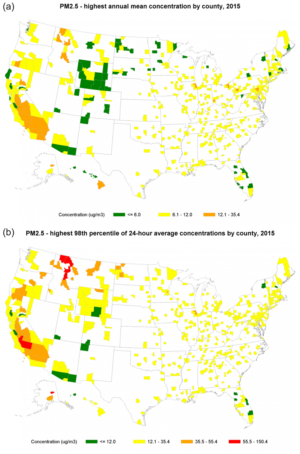
Figure 1(a) Annual average PM2.5 (24 h average) by county as observed for 2014 (source: EPA: “What is particle pollution and what types of particles are a health concern?”; https://www.epa.gov/pmcourse/what-particle-pollution, last access: 1 October 2019). The original description reads as follows: “US counties with high annual mean particle pollution concentrations in 2015. This map depicts fine particle pollution concentrations by US county for 2015 based on long-term (annual) average concentrations. The map's color key is based on categories of the Air Quality Index (AQI) (see Patient Exposure and the Air Quality Index). All orange and red areas exceeded the annual ambient air quality standards for fine particle pollution during 2015.” (b) The 98th percentile concentrations by count for 2014 from the same source. The original description reads as follows: “All orange and red areas exceeded the 24 h ambient air quality standards for fine particle pollution during 2015. The map illustrates how likely it may be for a particular area to experience air quality advisories for particle pollution based on short-term averaging.” The San Joaquin Valley comprises the area in red and the adjoining counties to the northeast and southwest; details are shown in later maps.
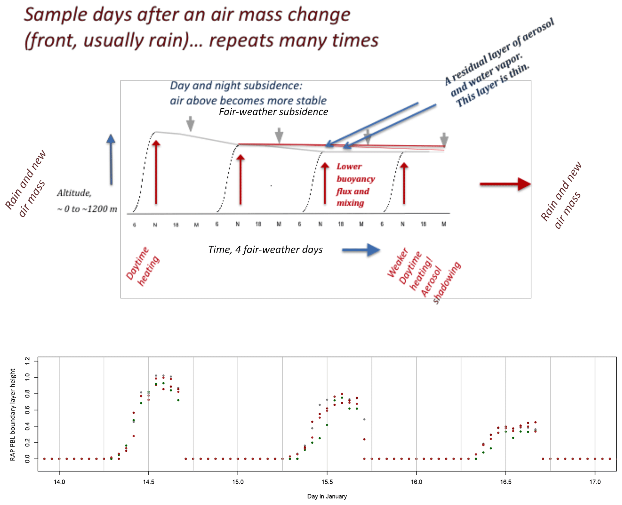
Figure 2(a) Conceptual figure describing the fair-weather planetary boundary layer (PBL) top for successive days in a clear-weather PM2.5 episode motivating this study; see text. (b) Simulation in the National Oceanic and Atmospheric Administration (NOAA) Rapid Refresh (RAP) model of PBL height for momentum at three SJV PM2.5 stations (red: Tranquility, gray: Hanford, green: Bakersfield). Periods from 11:00 to 15:30 UTC approximate the mixed layer for that period and time following, although advection may change the concentrations mixing to that height. Maximum PBL-top altitude may not be accurate for the station, but the shape of diel profile is appropriate.
More broadly, atmospheric PM pollution in the respirable range, PM2.5, has been recognized as a major threat to human health for some time (Brunekreef and Holgate, 2002; Dominici et al., 2006; Franklin, 2007; Kloog et al., 2013; Schwartz, et al., 1996; Zanobetti et al., 2009). Epidemiological studies have been hampered by the availability of relatively few PM2.5 measurement stations relative to the broad dispersal of populations affected. A variety of methods have been employed to estimate exposure, e.g., proximity-based methods using a geographic information system (GIS), interpolation between sparse monitoring sites, land-use regression models, line- or area-dispersion plume models, 3-D atmospheric source-and-transport models, and models using information from imaging satellites, often including also land-use regression and proximity (Sorek Hamer et al., 2016). Sparse PM2.5 monitoring spatial networks may limit our ability to accurately assess human exposures to PM2.5, since concentrations measured at an outdoor site may be less representative of the subjects' exposures as the distance from the monitor increases (Bell et al., 2007; Lee et al., 2011).
For this reason, there has been extensive development of techniques to make the best use of satellite-borne optical extinction, as seen from moderate-resolution atmospheric imagers. AOT is typically reported as a vertical column integral of extinction above the ground footprint observed. Methods using AOT to assess exposure to PM showed early successes, but certain regions remained very poorly characterized (Engel-Cox et al., 2004; Liu et al., 2009; Gupta et al., 2006; Koelemeijer et al., 2006; Hoff and Christopher, 2009). Engel-Cox (2004) found correlations of AOT with PM2.5 for valleys along the US Pacific coast that ranged from −0.2 to +0.3; i.e., very little variance is explained. Multi-angle Imaging SpectroRadiometer (MISR) technology aided greatly (Liu et al., 2007) but yields mostly monthly averages over years (van Donkelaar et al., 2010), limiting event and epidemiological analysis.
AOT may be strongly affected by particles encountered well above the planetary boundary layer (PBL) and different particulate composition. In addition, cloud cover severely limits the actual spatial coverage of AOT (Ford and Heald, 2016). Yet, in spite of these limitations (Jin et al., 2019), AOT has been employed extensively for assessing PM concentrations (e.g., Liu et al., 2018; Franklin et al., 2017; van Donkelaar et al., 2015, 2016; Kloog et al., 2015, 2014; Hu et al., 2014; Sorek-Hamer et al., 2013; Hoff and Christopher 2009).
In regard to the SJV, considerable work has been published, since it was the site of two major intensive studies: CRPAQS (California Regional PM10∕PM2.5 Air Quality Study; Chow et al., 2006) and DISCOVER-AQ California (Deriving Information on Surface Conditions from COlumn and VERtically Resolved Observations Relevant to Air Quality; https://www-air.larc.nasa.gov/missions/discover-aq/discover-aq.html (last access: 1 October 2019); more references below and on the web site). There was a very useful analysis of particle composition for a well-instrumented Fresno surface site for this period (Young et al., 2016). This study added detail to the Watson and Chow (2002) analysis of an earlier intensive study of the area, in particular, the striking dominance of nitrate and organic aerosols in a regular diel pattern. Watson and Chow reference several publications describing that intensive study. Johnson et al. (2014) made a three-dimensional modeling study of methane emissions that also helps describe the mixed layer of the specific DISCOVER-AQ period. Lidar gives a very helpful view of complexities of submicron particle abundance and properties within the mixed layer and the uniformity of the mixed layer top (Sawamura et al., 2017).
Application of modeling with satellite AOT columns from different satellite platforms for the DISCOVER-AQ (included within our study period) was able to achieve R2∼0.8). These results were achieved for just the DISCOVER-AQ period of ∼6 weeks and with separate subregions of the central SJV. They highlight the complexity of composition and source-driven simulation (Friberg et al., 2018). The Friberg publication is highly recommended as a comparison to this effort and has extensive references regarding the SJV and the details required for source-driven modeling.
There are several related goals in producing PM2.5 maps and assessing their accuracy. The work of Friberg et al. (2018) primarily aimed to constrain the Community Multi-scale Air Quality model (CMAQ) downwind of the surface air quality stations and, in particular, to constrain particle type as much as possible, along with concentration, using MISR constraints (Ralph Kahn, personal communication, 2019). Our goal was to produce a large set of maps characterizing one winter in a particular setting, inland Mediterranean valleys, with the aim of allowing air pollution professionals to understand particulate episodes and to improve sources and simulation details (e.g., transport error) for source-driven models. Goals of the Dalhousie group are to improve annual average exposure: they see that as the principal driver for health effects (van Donkelaar et al., 2010, 2015, 2016). A main goal of NASA's Multi-Angle Imager for Aerosols (MAIA) mission is similarly deliver new data for an each-day mapping of PM2.5 exposure sufficient for full studies of health effects (Diner et al., 2018, https://maia.jpl.nasa.gov/, last access: 15 November 2019). In pursuit of that goal for the Moderate Resolution Imaging Spectroradiometer (MODIS) Aqua dataset, we will indicate some preliminary, meteorology-based ideas for estimating high aerosol concentration when clouds prevent the use of remote sensing data.
Due to the complex meteorology of the San Joaquin flows and uncertainties surrounding the sources of ammonia, nitrogen oxides, and residential-burning smoke, we attempt to separate out some certain aspects of complex 3-D source-driven modeling (Bey et al., 2001; Nolte, 2015; Appel et al., 2017; Friberg et al., 2018) with a “static model” which does not attempt to simulate transport but rather uses observational records related to vertical mixing and AOT. The spatial maps produced can give a more detailed check on the 3-D process modeling. They also allow the whole MODIS record of winters to be analyzed efficiently so as to reveal patterns and trends. We emphasize this and further extension the interpretation of satellite radiances, attempting to remain close to physical interpretations by using both multi-angle implementation of atmospheric correction (MAIAC) AOT and column water vapor (CWV) retrievals. MAIAC CWV (Lyapustin et al., 2018) retrievals have been quite acceptability validated with the AErosol RObotic NETwork (AERONET) CWV measurements in higher CWV environments (Martins et al., 2017, 2018). It has not been previously recognized as a tool for improving ground PM estimation and, in particular, in the SJV.
1.1 Data
1.1.1 MAIAC AOT and CWV
MAIAC is an operational algorithm developed for MODIS Collection 6 (C6) data (Lyapustin et al., 2011a, b). This algorithm applies a dynamical time series technique to derive the MODIS surface bidirectional reflectance factor and atmospheric retrievals at a 1 km resolution, such as AOT, and CWV (Lyapustin et al., 2008, 2011b). MAIAC AOT retrievals present an expected error within 15 % and relatively good correlation coefficient (R) with AERONET measurements in the study area (Lyapustin et al., 2018).
MAIAC data have been used from both Terra and Aqua satellite with a daily overpass at ∼10:30 and ∼13:30 UTC (+ ca. 1.5 h), respectively. Data have been obtained for the period of winter 2012–2013 (November 2012–April 2013). We surveyed this entire period and included, for estimation, all wintertime high-PM2.5 episodes for this specific winter, selecting 19 November–18 February, as described in several later figures (discussed in context: Figs. 3, 4, and 7).
1.1.2 AERONET AOT and CWV
AERONET is a global network of automatic Sun-and-sky radiometers for aerosol monitoring (Holben et al., 1998). Direct Sun measurements are used to compute the AOT values at seven wavelengths (340, 380, 440, 500, 675, 870, 1020 nm), while CWV retrievals are derived from the 940 nm channel (Schmid et al., 2006). The AERONET data were obtained for the study period with cloud-screened and quality-assured at V3 Level 2 products. The AERONET AOT values were interpolated to 550 nm using quadratic fits on a log–log scale. Details on instruments and monitoring sites of the DISCOVER-AQ campaign are available at: http://www.nasa.gov/mission_pages/discover-aq/instruments/index.html (last access: 1 September 2019). Archived DISCOVER-AQ data are available on the NASA LaRC Science Data for Atmospheric Composition website: http://www-air.larc.nasa.gov/ index.html (last access: 1 September 2019).
1.1.3 Ground PM2.5 concentrations
Hourly ground PM2.5 concentrations were obtained from the US Environmental Protection Agency (EPA) at ±60 min from the satellite overpass. Data were obtained from stations that reported non-negative PM values over the whole study period (https://aqs.epa.gov/aqsweb/airdata/download_files.html#Raw, last access: 15 August 2019).
1.1.4 PBL
Momentum-based PBL depth, 10 m wind, and some CWV quantities for the model were taken from the archive of the National Oceanic and Atmospheric Administration (NOAA) Rapid Refresh (RAP) model available for this period. (The choice of MAIAC or RAP estimates is discussed later.) The model archive had a nominal 13 km resolution resolved at a 1 h time interval, so that model quantities could be matched closely to the satellite overpass times. Unreported examination of the AERONET data for the period suggested that the temporal resolution of the MAIAC AOT was quite accurate. The High Spectral Resolution Lidar 2 (HSRL2) aerosol data as described by Sawamura et al. (2017) suggested that depths of afternoon mixing tops were adequately described by a 13 km resolution model, as were adjacent spirals of the NASA P3-B aircraft as described by Michael Shook (Shook et al., 2013; see also the Supplement). AOT could however vary on relatively short distance scales, e.g., within 0–2 km of roadways when winds were parallel to the road. We shall see the consequential variations in estimated PM2.5 later in the processed results.
Koelenmeijer et al. (2006) give a succinct description of the relationship between AOT and dry particle mass. We adopt their simplification describing the relationship of AOT to PM2.5 using a simple equation where all particles are idealized as evenly mixed throughout a layer mixing to sensors near the ground, and the thickness of the mixed layer is ΔzML:
The factor in the denominator, M (for “magnification”), describes the relationship of the optical extinction to “dry particle mass smaller than 2.5 µm aerodynamic diameter” which is the motivated definition of PM2.5. (PM2.5 also has a definition of a US “Federal Reference Method” which is formulated to approximate the physical definition as closely as possible.) The factor M then is a function of particle composition and the extinction coefficients bExt associated with the components, one of which may be largely absorbed water. Particle composition and ambient relative humidity (RH) then interact with each other to determine the water content. It is significant that RH is a function of temperature and therefore altitude, with highest RH at the top of a well-mixed layer.
This work emphasizes and attempts to exploit features of regional aerosol haze palls that parallel features of aerosol mass and a different measure of water vapor.
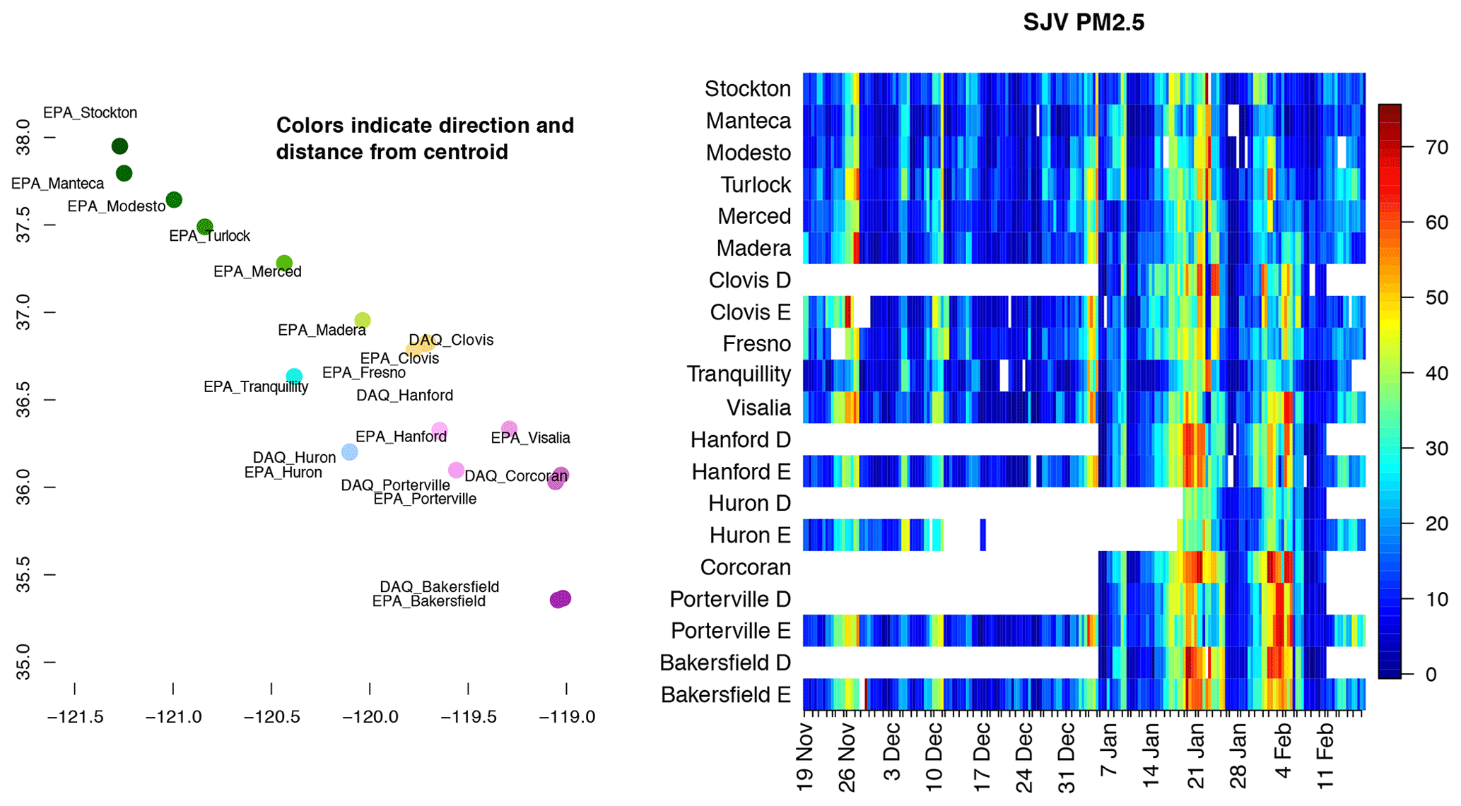
Figure 3(a) Locations of stations in the SJV used; color coding allows nearby stations to be identified. (b) Matrix plot of PM2.5 as measured at all instances of overpass at the sites for the period 19 November 2012 through 18 February 2013. The x axis has variable spacing in time; tick marks indicate successive days. Another view that summarizes the variability of observed PM2.5 is shown in Fig. 4a.
Figure 2 illustrates a conceptual idea of the fair-weather simulation that we focus on. Both regional particulate pollution and water vapor originate from the Earth's surface. Each tends to create relatively well-mixed layers over several days, transported most significantly by a repeated daily cycle of mixing. The mixing of momentum is most active from just before noon to the mid-afternoon, creating an afternoon mixed layer, and water vapor and aerosol most typically mix well up to this layer. Turbulent mixing depths vary from day to day, and these can create lofted layers of pollution cut off from the surface on the day of AOT and CWV observation. Flows in the SJV can be greatly influenced by the nearby mountains, with flows day and night, promoting some upslope transport of material which can recirculate, detached from mixing on following days. Consideration of subsidence of air into the San Joaquin mixed layer suggests a flow-through time for aerosol and water of 2–3 d for some situations (Caputi et al., 2018). Mixing of entrained and mixed layer air allows for continued accumulation of pollutant aerosol in the valley as Fig. 2 shows.
Particles and water vapor are emitted and accumulate in the same region, and they are mixed similarly each day at midday and in the afternoon by convective stirring. The height of mixing can be determined by variations in the buoyancy flux from the surface and varying vertical subsidence velocities, responding to larger-scale weather patterns, during successive days. Figure 2 does not show the effect of particle transport or water vapor transport for a specific location, but for the PBL top, which is strongly controlled by local heat and water vapor fluxes at the surface.
If the mixing height is lower on succeeding days, then any water vapor and any particles at the top of the mixed layer are trapped in an “elevated layer” which does not mix to the surface. Other common ways in which elevated layers can be formed are mixing along the side of the valley (small-scale anabatic and katabatic winds) and by differential transport, i.e., wind shear. Fires, power plant plumes, and long-distance synoptic transport can form layers that are quite separated at higher altitudes in the troposphere. Eventually, there is removal of both species. Wet removal of particles is particularly effective, and the specific humidity of the air is very effectively removed by the condensation accompanying cooling and rising, according to the Clausius–Clapeyron equation. Similar processes then limit the vertical spread of particles and specific humidity.
Water vapor molecules also accumulate in the atmosphere over a period of several days (typically a somewhat longer period), and both aerosols and water vapor are cleared from a particular place by cloud removal processes (venting, rainfall) and by air mass replacement. In the case of high-pressure systems in which air pollution episodes occur, such replacement is a common feature. If the other variables are available by measurement, e.g., airplane measurement such as in DISCOVER-AQ (https://discover-aq.larc.nasa.gov/data.html, last access: 15 August 2019), Eq. (1) can be solved for ΔzML, defining an equivalent mixing height for particles. Similarly, we can write equivalent mixing depth of water vapor, :
where CWV is in g cm2, and correspond to the vertically distributed water vapor and appropriately average water density of the mixed layer. CWV is available from the MAIAC analyses yielding AOT. Making the assumption that the heights are the nearly equivalent for water vapor and aerosol, we may write
PM2.5 is calculated at EPA reference temperature (25 ∘C) and pressure (1 atm), water vapor quantities in g cm−3, and in centimeters.
Work reported by Shook et al. (2018) described the vertical distribution of trace species with a vertical coordinate normalized to this estimated afternoon mixed layer top. This suggested to us that water vapor had vertical distributions that were usefully similar. The decline of water vapor was not as sharp, often showing a rapid decrease; the drop in scattering was dramatically rapid.
We found in ensuing work that approximating by () added only a small amount to the variance explained by the regression given other limitations of the approximation. (Possibly relative humidity effects or the correlation of water density with temperature could be complicating correlated factors.)
We calibrate the f(AOT) relationship using data at official PM2.5 stations and make the calibration daily. It is our observation that f varies only over a small range when there are several MODIS observations on the same day, and that it varies in a limited way between neighboring stations in a local region. The definition of “region” is based on that similarity, and it suggests similarity of ΔzML and M, i.e., similar aerosol characteristics and boundary layer behavior. This similarity does not apply when the wind shifts greatly between times or between stations, e.g., when a front passes. Fortunately for our understanding of pollution episodes, frontal passage days tend not to have high PM2.5.
We distill these understandings when we formulate a regression equation:
where the subscript i describes “instance” or calendar date, and subscript s describes “station”, so that AOT and PM2.5 form a two-dimensional table.
Given the independent nature of i and s, the regression must be solved by mixed-effects methods described below. The subscript s needs to only be independent of i, so later we will use it to denote “situation” or the hour of the day when there are many observations made at one station on one day i. It is not assumed that the consecutive order of the day observations necessarily describes any continuity in i. Observations show that there is often continuity, but that the continuity is quickly broken when frontal passages or rain affect the region.
Writing Eq. (3) in the form used for mixed-effects models, we separate a general term from the terms that depend on i or calendar date.
A commonly used shorthand is the Wilkinson and Rogers (1973) form, accepted by many software packages:
where DOY describes the calendar date subscript i. This formalism also describes the columns of the regression matrix to be solved.
It is tempting to generalize this relationship to recognize that there is often correlated behavior between stations but with some constant offset:
However, if one allows such variations at monitoring stations, it can be difficult to decide what values of γs to use between stations. This is an attempt to describe “subregionality”, that is, similar behavior within a region modified by slight and geographically coherent variations which allow spatial interpolation.
For those not familiar with mixed-effects models, we mention that the procedure is similar to the use of dummy variables, where coefficients ui multiply a set of discriminating variables, equal to 1 when i takes on the value of a particular instance/day, and 0 for all other instances. The mixed-effects techniques similarly solves a much larger regression equation but has better theoretical development. Note that the number of observations is Ni times Ns, while the number of parameters is linear in Ni and Ns, where N signifies the number of instances. When Ni and Ns>5, the problem becomes increasingly overdetermined.
This basic understanding does not fully explain the success of the mixed-effects model that we observed for the San Joaquin Valley. Furthermore, analyses of the Baltimore–Washington DC area not described here suggest that it works more broadly. Both aerosol and especially water vapor often exhibit layers not in continual contact with surface monitors. These we will call “elevated layers”. In situ measurements on aircraft and also lidar measurements from ground lidars looking downward from aircraft (Sawamura et al., 2017) and satellite lidar (Cloud-Aerosol Lidar and Infrared Pathfinder Satellite Observation; CALIPSO) reveal aerosol layers with significant optical thickness above the mixing layer. Similarly, airborne measurements in the DISCOVER-AQ intensive measurements of 2013 suggest a fraction of water vapor lies above the mixed layer for water. Allow these portions of total AOT and CWV layers to be quantified as AOTe and CWVe (“e” stands for elevated). There can be several individual layers. AOTe and CWVe refer to the total amounts of extinction and water vapor mass. Thus, there is an approximate equation upon which to base regression estimation:
While elevated layers of water and aerosol are common, we will see that it appears that this regression equation allows rather good fits. This can happen when AOTe≪AOT and CWVe≪CWV to a sufficient degree, or else when there are approximate linear (slope plus intercept) relationships obtaining between the numerator and denominator of Eq. (8). Essentially, the terms are absorbed into constant parameters for the day, αi and βi, along with other parameters like M. AOTe and CWVe are considered to be essentially constant over the region. In fact, this degree of constancy can be taken to define the “region” of application. Transforming these terms into constants, αi and βi, works under an implicit assumption of uniformity in AOTe and CWVe throughout the region or at least a uniform linear dependence with AOT and CWV.
In this section, we will show how components of a mixed-effects model that utilize CWV contribute to its explanatory power. We examine the relationships and predictive ability for PM2.5 observed at SJV measurement stations for the winter season encompassing high-pollution periods, 19 November 2012 to 17 February 2013. Stations from Bakersfield in the south to Stockton in the north were included. Figure 3b shows several episodes affecting most of the valley; one period with more stations reporting includes the DISCOVER-AQ period. This period has additional P3-B aircraft data which motivated this work but are too lengthy to describe in this publication.
Figure 3a shows the locations of all stations used in this work; the stations include much of the valley from Stockton to Bakersfield. Some of the stations labeled “DAQ” were in operation only during the DISCOVER-AQ California period. A color wheel was used to assign colors to the stations on the graph; this allows identification of stations' latitude, longitude, and proximity in later graphs comparing observations and our fitted values. Figure 3b describes the rise and fall of PM2.5 pollution using the station reports. The rows represent stations and are arranged north to south. Several major episodes are immediately seen, as well as differences in their intensity and timing of development. The DISCOVER-AQ observations were limited to the period shown, 8 January through 10 February 2013. Differences between the PM2.5 values observed at nearby stations, one DISCOVER-AQ and one California Air Resources Board (labeled “EPA” for the dataset origin), give an impression of local variability; differences between observations at Clovis are quite apparent.
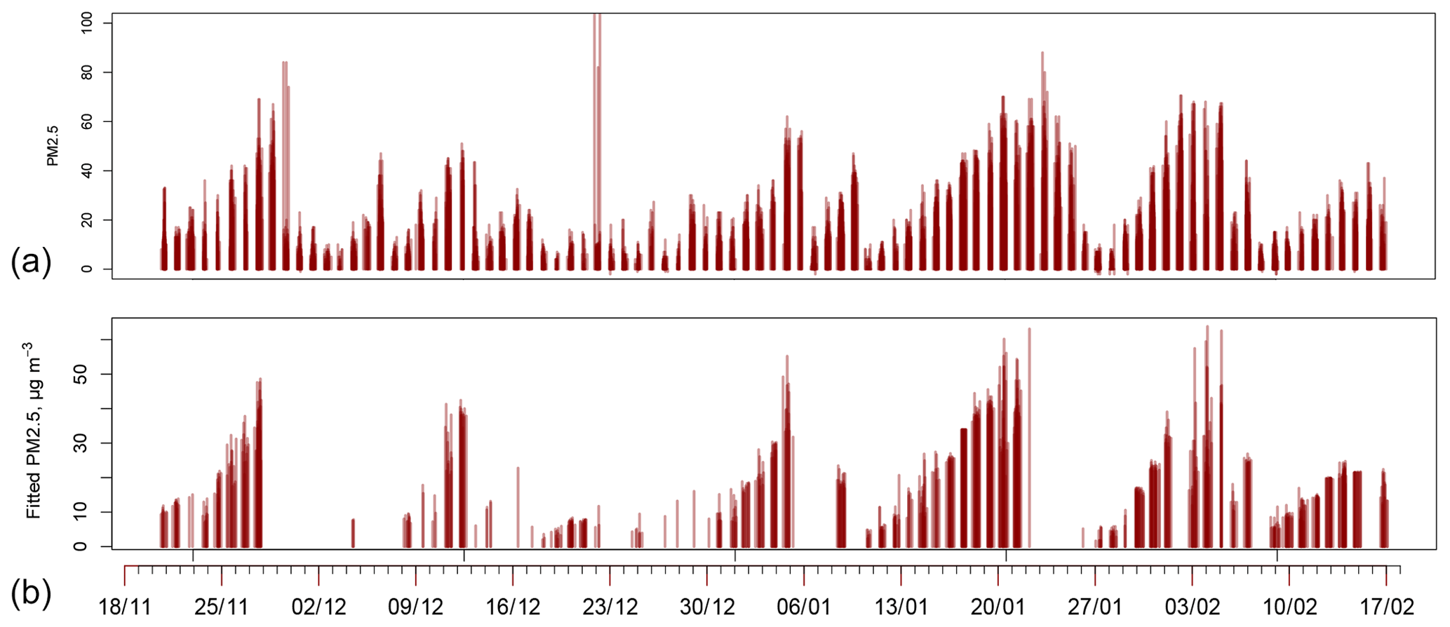
Figure 4(a) PM2.5 as observed at all stations for the winter period extending from November 2012 to March 2013. The graph has vertical bars drawn with partial transparency, so that careful inspection of a single day describes all the observations in the valley for the day. The observations contributing for each day may be seen in Fig. 3b. (b) PM2.5 as fitted by the regression with slopes and intercepts, described further below.
Using the MAIAC 1×1 km estimates for each day for the location of each aerosol monitoring station and the PM2.5 measured at overpass time for that day, we may solve the estimation equation (Eq. 6).
The complete simulation of PM2.5 measurement at all stations where MAIAC data allowed is shown in Fig. 4b. The technique can be used for all years and the whole area of the SJV where MODIS data are available. We used the complete model as described in Eq. (6), with “slopes” and “intercepts” but without any time-independent spatial variation allowed (γs). Three features deserve immediate comment. First, there are patterns of gradual increase of PM2.5 up to 45–80 µg m−3, followed by relatively sudden decrease to levels near 5 µg m−3. Second, the regression technique using AOT ∕ CWV, as estimated individually for each day, captures the variation rather well for all days where estimates can be made.
Individual exotic high values are not captured. Third, there is a pattern where the end of an air pollution episode, showing very high values, is not captured by the technique. These are simply days where MODIS observations were not available, almost always due to cloud cover. We expect that these are readily explained in terms of weather phenomena especially typical of the western US during wintertime. Pollution episodes are ended with the approach of warm fronts with high clouds, followed in a few days by the cleansing effects of rain, air mass replacement, and higher wind. We will return to this topic later.
To understand what information is used by the technique and the importance of that information, based on the series of regression estimates we presented, we argue that there is a cumulative aspect to the explanation. For example, when we include one statistical variable, e.g., αi, describing variation by day but constant for all stations of the day, then the regression with AOT ∕ CWV becomes much more informative. A general relation describing the slope of PM2.5 with AOT ∕ CWV becomes more useful when an appropriate intercept (offset) is provided.
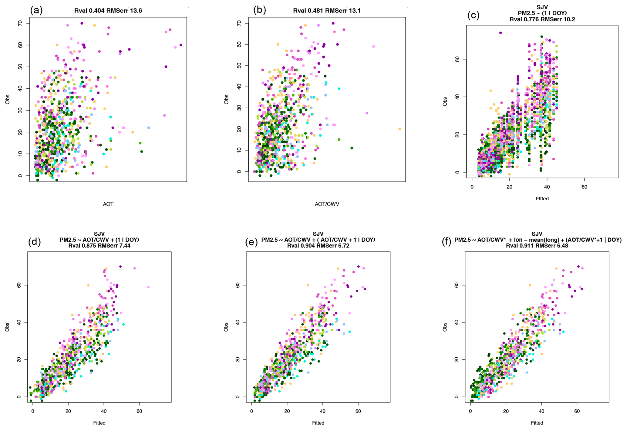
Figure 5Progressive improvement of PM2.5 simulation showing the roles of daily calibration and AOT ∕ CWV descriptions of aerosol vertical dispersion. Station observations (µg m−3) are shown on the y axis; estimators are shown on the horizontal axis. Note the progressive refinement of R and remaining root mean square error (RMSE); see text. (a) Use of AOT only, an early methodology. (b) Some improvement using AOT ∕ CWV but no daily calibration. (c) More improvement with daily calibration (mixed effects using intercepts αi). (d) Clearly improved linearity when combing intercepts with AOT ∕ CWV. (e) Estimating daily “random” intercepts and slopes improves RMSE and R. (f) A simple description of variation within the region (longitude) aids the estimation slightly (RMSE ∼6.48 µg m−3, R∼0.91).
Consider both Table 1 and Fig. 5 as they describe cumulative effects of adding information. First, we note that AOT alone is not very informative about PM2.5. This would seem to follow naturally from Eq. (1), since variations in mixing depth and composition are not considered. Figure 5a shows many station observations with high PM2.5 but low AOT, and vice versa. Slight but significant improvement is made when CWV is introduced to provide some information on mixing depth and dilution. R improves to 0.48 but the remaining error is nearly as high. Still, some linear relationship begins to show for perhaps 60 % of the data.
A side comment regarding significance: R and remaining root mean square error (RMSE) (in µg m−3) are shown in Table 1. We also performed two other tests that are not tabulated. An analysis of the Kullback–Liebler divergence (Hastie et al., 2009), where possible, suggested each successive test in the table clearly adds information regarding PM2.5. The number of observations justified the number of additional parameters. While the numerical values are difficult to compare to other examples of regression, they show similar trends to R and RMSE; i.e., accuracy becomes increasingly hard to improve as R increases. Another test was leave-one-out cross validation (Hastie et al., 2009). Each individual station was omitted, and the regression based on the remaining stations was tested against observations at that station. The cross-validated mean squared error was about 7.8 µg m−3 at most for the most informative regressions shown.
Table 1Comparison of results using different terms in the mixed-effects model.

(1) Variables are described in the context of Eqs. (4)–(8) in the text. (2) In all regressions with random effects (all but the first two regressions), the inclusion of the α and c variables suggests an overfitting. Mixed-effects convention emphasizes these “main effects” separately and therefore specifies there must be a single linear constraint on the terms such as α and αi (also, c and βi). Importantly, in Sect. 6 and certain figures below, we describe the (more intuitive) combination of main and random effects; e.g., we graph and .
Now consider a popular alternative to the use of satellite data. The third regression shown, labelled (1|DOY), omits satellite data and uses only a single value based on day of year to give a uniform-valued PM2.5 estimate for the whole region. As Table 1 shows, this can do significantly better than the previous non-mixed-effects regressions using satellite data. Color-coded maps of PM2.5 drawn for a region have a single color which varies from day to day. In many applications of satellite data to particulate estimation, this has been shown to surpass, or at least approximate, the results of use of AOT (Sorek-Hamer et al., 2017). R∼0.78, RMSE ∼10 µg m−3. Its success emphasizes the regional similarity of conditions defining PM2.5 concentrations and their extensive spatial correlation. An explanation is that respirable PM2.5 is defined by daily weather and orientation to major sources.
Once the regional similarity of pollutant conditions is recognized, it becomes appealing to combine information. The fourth estimate, Fig. 5d, does just this and shows a notable increase in R (0.88) and decrease in RMSE (8.03). This is an approximately 50 % decrease in error variance. In our situation, satellite data look to be useful. The scatterplot of Fig. 5d suggests distinctly more linear behavior.
An appealing alternative is to estimate only slope variations, βi. This is nearly as useful as estimating just αi, R∼0.85 RMSE ∼10 µg m−3. Each is useful. Do the two parameter estimations give distinct information?
Estimation of varying offsets αi and sensitivities αi does indeed help, reducing the variance by another 10 %. Combining the use of AOT, CWV, and individual daily intercepts and slopes yields R∼0.90 and RMSE ∼6.72 µg m−3. Nevertheless, Fig. 5e shows that certain stations have persistent deviations from the general swarm of points; Tranquility (pale green) is predicted high, and Porterville and neighbors (red) are predicted low.

Figure 6Estimated surface PM2.5 at 1 km indicated overpass times for the first wintertime episode in the San Joaquin Valley. Winds at 360 m a.g.l. are also shown. Estimated RMSE is 7 µg m−3 with a similar limit of detection. Filled circles show station PM2.5. In this episode, the E–W correction based on the full dataset appears inappropriate, lowering mapped estimates in the east valley. Error should decrease with improved understanding of geographic variability. The time stamp at the top of the image describes the date and time in UTC format.
This analysis of residuals suggests that there may be spatial variations that can be specified for our stations (γs) but are general enough that they can be extended to maps. For this publication, we attempted a very simple variation, an east–west variation (longitude). This did improve the scatterplot for most stations, especially when considering values above ∼10 µg m−3. RMSE decreased slightly to 6.48, and the R estimate also rose slightly to 0.911. These changes are close to the range of sample variability. The maps shown in Fig. 6 also show more convincing (subjective) agreement in magnitude and pattern. Nevertheless, many of the highest observations are underestimated by about 20 %.
We used CWV rather than the RAP planetary boundary layer height for momentum (11:00 to 15:30 UTC). This was available in the 2012–2013 winter at times within a half hour of overpass time; however, this PBL height is not always recorded in the high-resolution RAP archive. We compared a regression very similar to the most detailed regression of Table 1 but using this PBL height. The formula used was
With this, the R value was 0.917 and the RMSE was 6.25 µg m−3; these are only insignificantly better than the CWV-based estimate R of 0.912; the RMSE was 6.43 µg m−3. Mid-afternoon PBL depth is consequently useful. However, the CWV-based estimate may be used with all years of the MODIS data, while the best-available meteorology for PBL depth varies considerably, as high-resolution NOAA models advanced through the years.
The major purpose of this work is to combine AOT, CWV, and daily calibration in order to allow maps of estimated PM2.5 for all regions where MODIS can provide optical thickness data. Results using the full model with αi, βi, and γs are shown (Fig. 5f). Out of the 42 d in the calibration set, we consider 6 d of single major air pollution episode during middle of January 2013, a period that was largely sampled by the DISCOVER-AQ ground and airplane samples. Detailed comparisons of the DISCOVER-AQ data would expand this work beyond a manageable size; such analysis is desirable. Winds are shown with streamlines and are obtained by interpolation from the RAP wind analyses.
We created 39 maps, six of which are shown in Fig. 6. Their accuracy is good. RMSE is ∼7 µg m−3. This dictated the 5 µg m−3 contour colors used: similar colors or neighboring colors show expected agreement. Winds at 360 m for the hour of sampling have been superimposed on the maps.
There follows the description of just of one episode: on 14 January 2013, the valley is clean (see also Figs. 3 and 4). By 16 January 2013, light regional haze is accumulating, and the winds and mapped levels suggest some accumulation towards the south. On 18 January 2013, winds have veered: in the central valley, pollution accumulates towards the east; in the south, transport is towards Bakersfield. On 20 January 2013, winds press the accumulating PM2.5 back towards the more populated east valley. Several days following have increasing clouds (no maps). The first day, with advancing clouds overhead but no low clouds and no front nor rain, retains high PM2.5 at the monitors. This pattern is seen for several wintertime pollution episodes in this region. When the clouds clear, the valley is as clean as it was on 14 January. In the maps for 18, 19, and 20 January, the maps underestimate the highest values of PM2.5 by about 20 %, as noted above.
The well-performing mixed-effects models (Eqs. 5 and 6) led us to examine the repeated development of air pollution episodes to a maximum, striking patterns seen in Figs. 3, 4, and 6. How did the independent values for various models in Table 1 vary within episodes and between episodes? Our description of the development leads to some answers in Fig. 7.
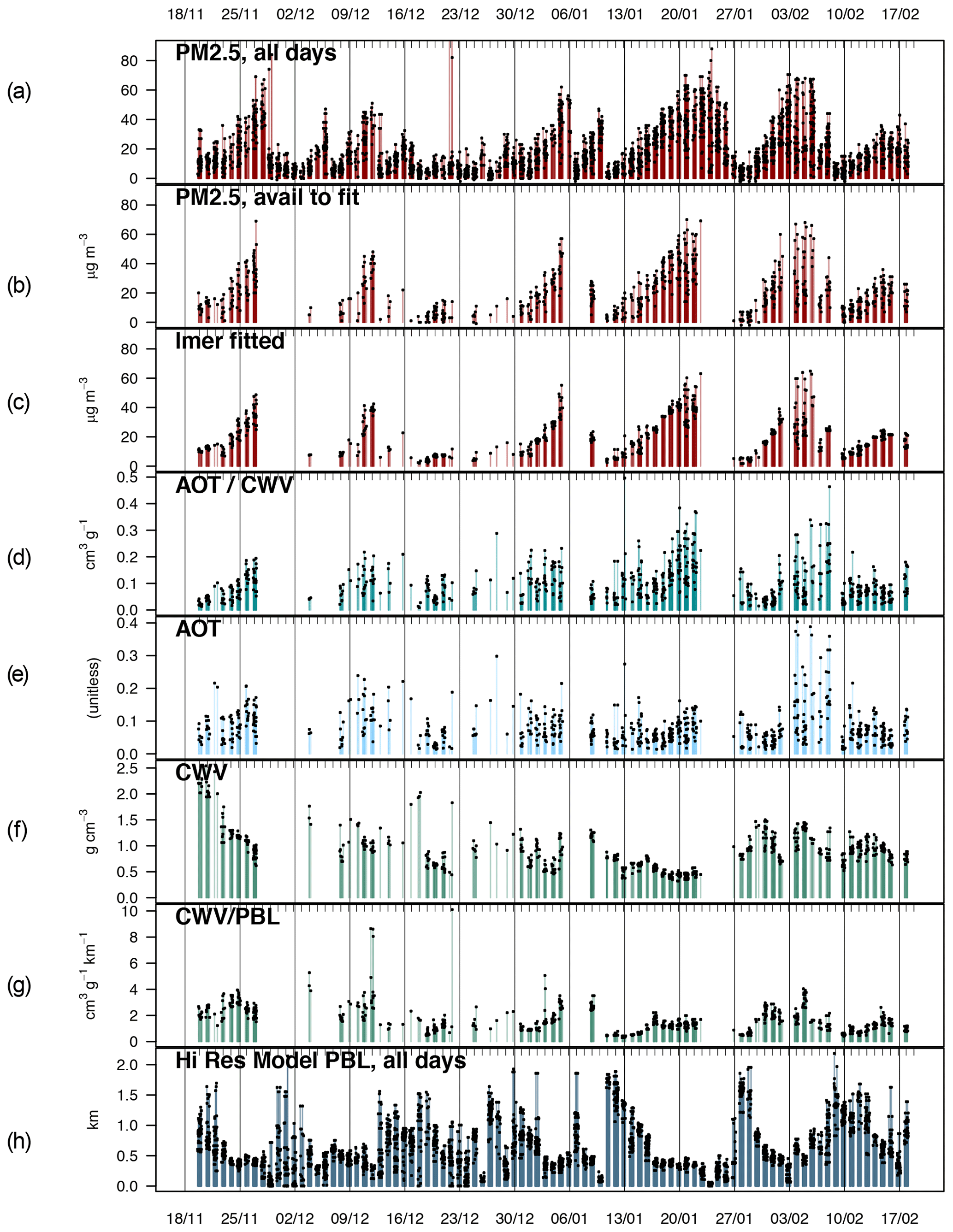
Figure 7Time evolution of PM2.5 and related variables for approximately eight intensifying particulate episodes during the winter of 2012–2013. Dots and vertical bars indicate variable values at individual stations when available. Blank regions reflect periods of cloud cover. (a) PM2.5 (µg m−3) as observed at stations (all dates) and (b) fitted PM2.5 on days and locations when MAIAC was available. (c) MAIAC AOT, 11:30 to 15:30 UTC. Note that the increase is less pronounced than PM2.5 and varies between episodes. (d) CWV in g cm−2 or, colloquially, “cm of precipitable (liquid) water.” (e) PBL height for the noon–afternoon observations in this dataset. Morning PBL heights are much lower. (f) Ratio of CWV to PBL height (cm(H2O-liq) km−1). The ratio remains relatively constant over several days, consistent with a commonly close meteorological relationship of CWV and PBL.
Figure 7a and b describe the development of the episodes. The time series of observed PM2.5 and fitted PM2.5 are repeated from Fig. 4. The times with no data are essentially cloudy times. After periods of cloudiness, particulate values typically rise until the next period of clouds. There are seven to eight such periods of rising, or weather episodes. (“Episodes” can also refer to periods of highest particulate matter.) High values typically remain for 1–4 d after cloud obscuration. Figure 7b and c show the values fitted by our mixed-effects regression and the values that are available for fitting. The time sequence as well as the magnitudes are in expected agreement, but the variability between stations is smaller on some occasions (e.g., 17 January and 15 February). Figure 7d shows that the time series of the AOT ∕ CWV ratio develops from day to day as PM2.5 does but suggests that these are modulated by differences in amplitude between weather episodes and sometime over several days within the weather episodes, e.g., 13 January to 17 January and 4 February to 8 February. These explain the low overall correlation. In contrast, AOT shows little resemblance in the time series. CWV shows some tendency to decline during weather episodes (Fig. 7e); notably, the values at different stations are more similar than those for AOT. Region-wide similarity in CWV within and above the afternoon mixed layer is an appealing explanation. Note the limited variability of the ratio of CWV to PBL over 3–5 d and between stations. The afternoon PBL height itself is shown in Fig. 7g. Note that it is often very low at the end of a cloudy period and then rises to high values ∼1 km at the end of the cloudy period. We suggest that this reflects overcast skies and very limited convective mixing, followed by rain and the introduction of new air masses with deeper mixing of water vapor in a less stable atmosphere.
Figure 7 describes differing causes of repeated PM2.5 buildup during cloud-free weather episodes. Progressive restriction of vertical mixing during clear-weather episodes acts to concentrate the effects of accumulated and recent pollution sources. The less stable air following a frontal passage feels increasing effects of strong subsidence, diminishing the mixing height. The 3-fold reduction in PBL height during major episodes (Fig. 7d) nearly matches the 4-fold increases in PM2.5 during these periods (Fig. 7a). MAIAC AOT shows variability between stations and is reflected in local PM2.5. Winds redistribute particles and AOT. Figure 7 does not make clear the fate of aerosol, but it likely escapes with mountainside winds along the valley. The entire set of maps suggests a flow to the south and stronger outflow near the Tejon Pass east of Bakersfield. These mountainside winds likely may facilitate water vapor and aerosols escape the prevalent mixed layer.
This suggests a typical behavior for the SJV and similar regions in winter. A cloudy disturbance (new air mass, rain, wind) stirs the lower troposphere. This initiates a high PBL mixing on the first clear days. Typical fair-weather subsidence begins. The surface buoyancy flux is too weak to maintain these relatively high mixed layer tops. Afternoon PBL depths and mixed layer depths decrease day by day until a depth of 300–400 m is reached (Fig. 7d). Escape from the valley may slow, allowing accumulation of pollution from within the region or from upwind. This further increases the surface PM2.5. Relatively local sources add to both AOT and PM2.5, and can transport them 50–100 km downwind, occasionally from east-valley sources to west-valley pollution hotspots (the map of Fig. 6d). Both subsidence and surface buoyancy flux are broad-scale weather phenomena (∼300 km) , and so AOT–PM2.5 relationships are similar on a given day with a given history of weather. Finally, warm-frontal rain approaches the region.
An examination of HSRL2 data for the DISCOVER-AQ period (Sawamura et al., 2017) suggests that there can be considerable vertical variability of aerosol extinction; the fact that AOT tends to average the whole afternoon mixed layer allows our generalized description to hold nevertheless.
Finally, we venture on to some ideas for filling in afternoon PM2.5 on days when MAIAC did not allow mapping due to cloud cover. Young et al. (2016) provided a thorough microphysical and chemical analysis for just the time period of 13 January to 11 February 2013 – essentially the DISCOVER-AQ period – and just the fully instrumented UC Davis site deployed in Fresno. Their Fig. 2a, b, and e show time series of temperature, wind speed and direction, and particle mass for the period, respectively. Their measurements include periods of cloud cover and clearly show air mass transitions during rain and frontal passage (seen as wind shifts, commonly N to W to S). These time series suggest a meteorological plausible method to interpolate PM2.5 maps into cloud-covered days. These do compare to our Fig. 7a, b, and c, describing observed and statistically estimated particulate mass at all stations including Fresno. PM2.5 drops to values below 10–15 µg m−3 whenever wind speeds rise to above ∼2 m s−1 and the wind direction is from a quadrant (90∘ sector) centered on the north–northwest direction. Their Fig. 2a also describes rainfall at the Fresno site. Particulate matter does drop by ∼50 % from the highest observed/estimated values at the end of the clear-sky period and further when the winds rise to 2 m s−1 or higher. This behavior is most clearly observed in their graphs for the period of 23–27 January. Similar behavior is observed in the period of 6–11 February, although the episode has a more complex increase than the earlier, most intense episodes. The short spike up to 80 µg m−3 on the night of 10 February is not explained and not reflected in the afternoon-only data of our Fig. 7. Nevertheless, the averages shown by Young et al. (2016) in their Fig. 2e do repeat the general observation that daily average PM2.5 and afternoon PM2.5 do tend to correlate well. For best-estimate maps of PM2.5, we suggest that the end-of-retrieval values of PM2.5 reduce gradually over a day or two. Maps of precipitation (e.g., from radar or other analyses) allow more detail. Estimates for a region should then fall to ∼7 µg m−3 whenever sustained winds rise to >2 m s−1 from the NNW or >3 m s−1 from any direction. Such wind speeds are held to mark air mass replacement (e.g., frontal passage). These ideas remain suggestions since our analysis for a single winter may not provide enough instances. The whole Aqua MAIAC period is available but currently beyond NASA's resources.
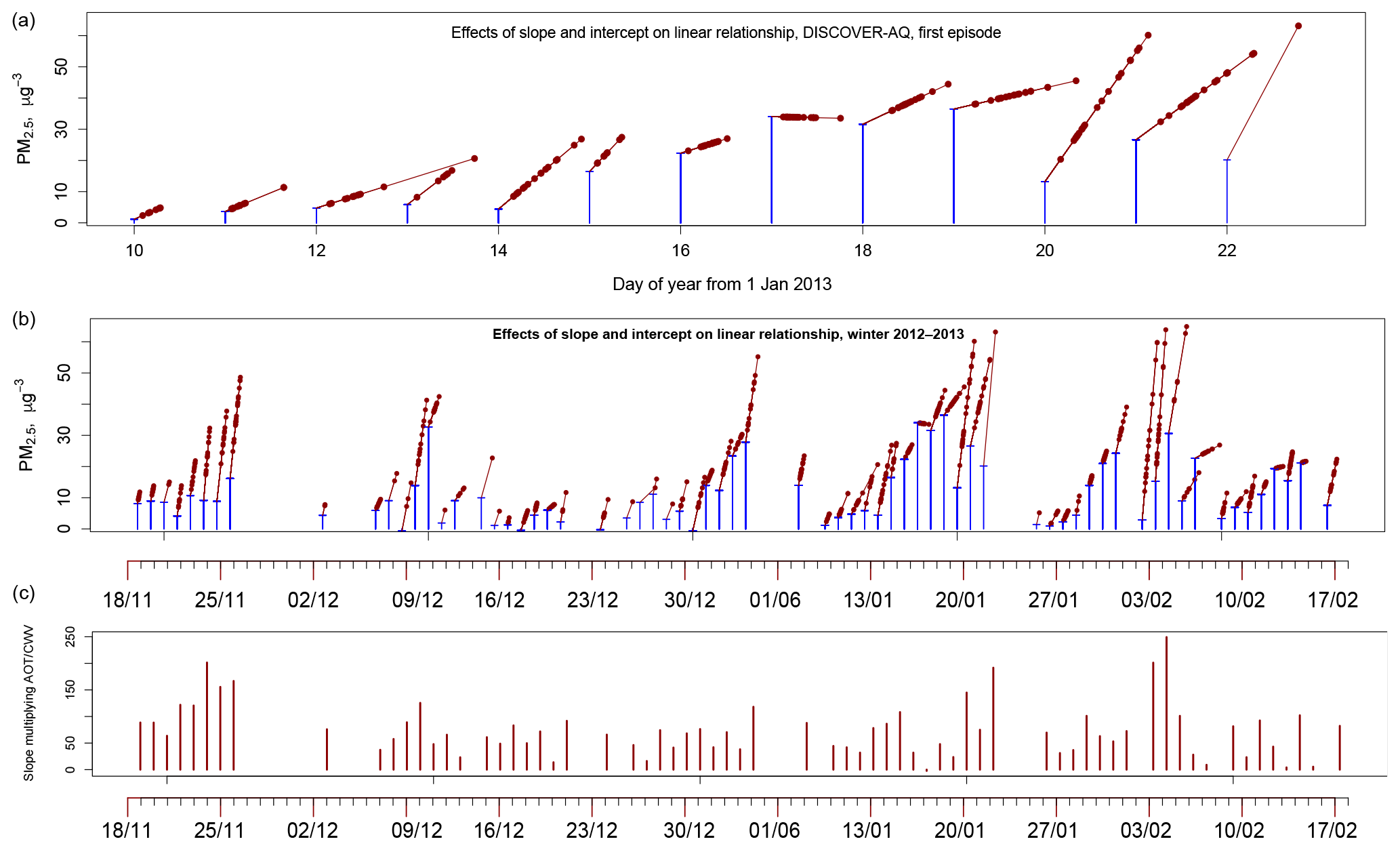
Figure 8Roles of slopes and intercepts in a regression fit. (a) A “stork plot” for the clear-sky air-pollution episode mapped in Fig. 6. Vertical blue lines indicate the contribution of the random intercept αi to the total PM2.5 fitted in the model. These are the same for all geographical locations including the observation stations for any given day. The slope parameter βi is the same for all geographical locations. (See note to Table 1.) Values of PM2.5 evaluated at the stations are shown by red dots along a line. Large values of AOT ∕ CWV have wide vertical extent, and the corresponding high values of PM2.5 are shown as red dots at the upper right of each day's plot. Highly sloped lines indicate high βi. (b) A stork plot for the whole wintertime interval evaluation, showing several clear-day episodes. (c) The values of βi vary considerably. These slopes are shown as a time series.
The preceding section gives some background so that we may understand the parameters for the random-effects model. We will discuss the full Eq. (4); results with mild spatial dependence (Eq. 5) are very similar. The intercept αi and the slope for are the same for each day and determine the fitted PM2.5 for the regression (Eq. 4). We exploit this to produce a “stork plot” like that in Fig. 8. High αi is shown by tall blue lines; high βi is shown as a high slope. Variation in AOT ∕ CWV contributes ∼30 %–70 % to the estimate on almost all days.
The stork plot in Fig. 8a illustrates a puzzling progression of parameter estimates day by day. For the first days (10–14 January), the slope parameter accounts for the largest contribution to PM2.5. For the second part of the period (15–19 January), the intercept term becomes progressively more important compared to the AOT ∕ CWV dependence. The regression equation fit (Fig. 7c) has difficulty in matching the observed PM2.5 (Fig. 7b) variability between stations on these days although AOT (Fig. 7e) shows moderate variability around low values (0.03–0.05). (A side note: MAIAC AOT estimates should be particularly challenged at these low values.) Then, from 20 to 22 January, the intercept contribution diminishes and the AOT ∕ CWV dependence becomes rather larger than typical. Referring back to Fig. 7e, f, and g, these variations seem explainable: the mixed layer decreases rapidly during the first period, then reaches a minimum at ∼300 m. In the last 3 d, the AOT increases rapidly, though the mixing depth changes little. The following weather episode is notable for high and quite variable AOT (Fig. 7e), and the fitting procedure does well.
At this point, concerns about the quality of the CWV estimate should be addressed. In our analysis of the difficult San Joaquin Valley, MAIAC CWV can be frequently low compared to AERONET CWV, some error can arise from the presence of clouds in neighboring footprints. In the figures and results, the shown CWV was based on the MAIAC data interpolated and extrapolated where cloud contamination made the retrieval of lower accuracy (Lyapustin et al., 2018). Figure 6 shows that some small-scale variability RAP analyses of CWV could also be used at their 13 km model-imposed width with similar results, since CWV does not vary as rapidly spatially as AOT. A better direct use of the MAIAC CWV could uses spatial averaging with a width of 3 to 6 km. Random errors in the MAIAC CWV due to the low radiances used would be reduced; considerations of source patterns suggests that CWV might not truly vary at such small scales. Improved PM2.5 values could result. We are implementing this averaging.
As understanding of MAIAC CWV improves, its role in determining daily AOT–PM2.5 relationships should improve; calibration of MAIAC using Sun photometer measurements can be useful in the meantime (Just et al., 2019). Note also that assimilated CWV from the National Weather Service models is constrained empirically by satellite and surface observations, and therefore CWV is not as reliant on transport descriptions as is aerosol. Here, some constraints are surface-station humidity measurements constraining CWV below 0.4–1 km; thermal-radiation sounders on the GOES (Geostationary Operational Environmental Satellite) satellites describe water vapor partial above that; radiosonde and GPS humidity sensors give further constraints. This allows GOES AOT estimates to be used with assimilated CWV, even though GOES lacks a reflective water vapor channel (Shobha Kondragunta, personal communication, 2018).
As our goals, we sought broadly applicable methods to estimate PM2.5 maps from satellite AOT for very polluted regions poorly described by satellite data. This study focused on the whole polluted winter season of the SJV (19 November 2012 to 18 February 2013). We sought to fulfill the overarching goal of the whole DISCOVER-AQ mission – to find general relationships between extended satellite data observations and surface air pollutant concentrations and to evaluate their success. We found success with a simple methodology that follows the meteorology of regions like the SJV. This success recommends an approach to the remote sensing to PM2.5 analysis, investigating important pollution regions in terms of their meteorology and sources but carrying over methods from similar regions. For example, the Po Valley of Italy and the Indo-Gangetic Plain of India may respond similarly to analyses based on detailed mixing height data and related distribution indicators.
As direct results, we found that a combination of information utilizing (1) optical depth, (2) measures of vertical dispersion (e.g., CWV), and (3) daily calibration of PM2.5 to predictors produced significantly better quantification of PM2.5 than a competitive no-satellite-use method which we named “regional correlation” since it produces unfeatured maps of PM2.5 which vary only from day to day. Our maps of estimated PM2.5 extend for all cloud-free periods from 19 November 2012 to 18 February 2013, which is essentially the whole pollution season for this winter. For that whole period, this first published attempt found good predictive value of R∼0.9 and RMSE of 6.5 µg m−3. Cross validation suggested an RMSE of 7 µg m−3. Analysis of residuals suggested that better RMSEs could be achieved if further work allowed for subregionality (use of smaller regions or a geographic characterization incorporating some spatial variation). Local variations in PM2.5 on the order of 1–3 km were noted using our method but only when particulate accumulation could occur along-wind. Still, in order to estimate PM2.5 at 1 km scales, we expect that it will be necessary to use refined geographic information system methods (Kloog et al., 2014).
DISCOVER-AQ comparisons are advisable. Our analyzed winter 2012–2103 period did include the more limited DISCOVER-AQ California 2013 airborne-intensive study period, primarily focused on the area around Fresno. Analysis of that intensive period suggested ideas (Shook et al., 2013) that motivated this work. The shorter DISCOVER-AQ period does deserve more detailed comparison to our results. Aircraft in situ profiles of gas and particle composition, lidar profiles, very detailed surface measurements of particulate composition, and source-and-transport modeling all deserve comparison. The distribution of atmospheric particles and precursor gases is more complex than this work might suggest. Somehow averaging appears to allow our general methods. The development of concepts and the length of this work do not allow for such comparison. We hope that research will be encouraged.
A major finding was that the usefulness of CWV does not become apparent unless there is daily calibration of the AOT ∕ CWV relationship to PM2.5. We attribute this primarily to (a) details of CWV (e.g., CWV's dependence on mixed layer temperature on the timescale of days), (b) CWV above the mixed layer for aerosols, presumably responding to other H2O sources upwind, and (c) variations in composition (the relation of PM2.5 to light extinction). We believe that allowing for a full linear relationship each day for AOT ∕ CWV to PM2.5, both slope and intercept effects, in a daily calibration allows regression to exploit portions of the PM2.5 vs. f(AOT ∕ CWV) scatterplots that reveal proportionality. High-spatial-resolution estimates of the 11:00–15:30 UTC PBL heights for momentum may be as helpful as CWV when available and when the PBL estimation has been examined for accuracy; this could be explored. Such PBL data are not available for the whole MODIS Aqua period (2004–present), while CWV data are.
In terms of accompanying insights on pollution episodes, we found that this approach allowed a broad description of the buildup of six air pollution episodes and the balance of the roles of accumulation of pollutants vs. limited vertical mixing. Episodes were as in earlier descriptions (Watson and Chow, 2002). Each appears important in different phases of repetitive PM2.5-increase cycles. PM2.5–AOT relationships suggest a few days' residence time for particles (actually particulate extinction) in the valley. The first 1–3 d after MODIS described full cloud cover could still show high, slowly decreasing PM2.5. Unpublished analysis (see Young et al., 2018) suggests that this high PM2.5 dropped precipitously when surface winds rose to >4 m s−1 from a quadrant centered on the NNW.
Best-estimate extensions to cloudy periods of the remote-sensing-based record can be made using the typical meteorology of the SJV or presumably other areas, and verified by extensive checks. Widely available data mapping surface winds and precipitation suffice and do not require detailed meteorological modeling to be available.
In terms of the role of “static” models, our estimation approach aimed to avoid the use of modeling driven by source estimation and transport simulation. Principally, we wished to provide datasets that allowed independent comparison to such 3-D atmospheric chemistry models (e.g., Friberg et al., 2018). When we used RAP-model CWV rather than spatially averaged or calibrated (Just et al., 2019) MAIAC CWV, that goal was not fully reached, although RAP CWV is strongly constrained by surface, satellite, and other observations. An aspirational goal is to provide an economical, accurate, and calibrated estimation of PM2.5 for the whole MODIS Aqua period to date and then beyond. The opportunities to use MISR, Visible Infrared Imaging Radiometer Suite (VIIRS), MAIA, and even geostationary imaging are appealing!
MODIS data with MAIAC processing is accessible via Lyapustin et al. (2018). The database of PM2.5 measurements (Federal Reference Method) is accessible via Environmental Protection Agency (United States), 2019. The estimation method for the mixed effects estimation is available from GitHUB: https://doi.org/10.5281/zenodo.3625240, Chatfield, and Esswein, 2019.
The supplement related to this article is available online at: https://doi.org/10.5194/acp-20-4379-2020-supplement.
RBC was responsible for conceptualization. AL and RE were responsible for data collection. RBC and RE were responsible for data analysis and modeling. RBC and RE were responsible for visualizations. RBC and MSH were responsible for writing and validation.
The authors declare that they have no conflict of interest.
We gratefully acknowledge the support from NASA's DISCOVER-AQ mission, followed by very encouraging continued interest and some partial support from the Health and Air Quality program management of NASA's Earth Science Applications Division. This allowed fulfillment of the prime DISCOVER-AQ objective to demonstrate the relevance of remote sensing to specific air pollution problems. We appreciate the advice from individuals in that program's Applied Science Team and from the GEO-CAPE mission formulation effort (aerosol focus). Aid from Yujie Wang (NASA GSFC) regarding the MAIAC processing of MODIS data was helpful. Michael Shook's analysis suggested the use of CWV. Recent comments on the draft paper by Qian Tan and Frank Freedman are also appreciated.
This research has been partially supported by the US NASA Earth Sciences Research program (NNH09ZDA001N-EV1) for the DISCOVER-AQ suborbital mission, with additional support by the NASA Earth Sciences Applications Health and Air Quality program. The work of Alexei I. Lyapustin was funded by the NASA Science of Terra, Aqua, and SNPP programs (17-TASNPP17-0116; solicitation NNH17ZDA001NTASNPP).
This paper was edited by Michael Schulz and reviewed by two anonymous referees.
Appel, K. W., Napelenok, S. L., Foley, K. M., Pye, H. O. T., Hogrefe, C., Luecken, D. J., Bash, J. O., Roselle, S. J., Pleim, J. E., Foroutan, H., Hutzell, W. T., Pouliot, G. A., Sarwar, G., Fahey, K. M., Gantt, B., Gilliam, R. C., Heath, N. K., Kang, D., Mathur, R., Schwede, D. B., Spero, T. L., Wong, D. C., and Young, J. O.: Description and evaluation of the Community Multiscale Air Quality (CMAQ) modeling system version 5.1, Geosci. Model Dev., 10, 1703–1732, https://doi.org/10.5194/gmd-10-1703-2017, 2017.
Ballard, M., Newcomer, M., Rudy, J., Lake, S., Sambasivam, S., Strawa, A. W., Schmidt, C., and Skiles, J. W.: Understanding the correlation of San Joaquin air quality monitoring with aerosol optical thickness satellite measurements, ASPRS Annual Conference, Baltimore MD, 2008.
Bell, M. L., Ebisu, K., and Belanger, K.: Ambient air pollution and low birth weight in Connecticut and Massachusetts, Environ. Health Perspect., 115, 1118–1124, 2007.
Bey, I., Jacob, D. J., Yantosca, R. M., Logan, J. A., Field, B. D., Fiore, A. M., Li, Q., Liu, H. Y., Mickley, L. J., and Schultz, M. G.: Global modeling of tropospheric chemistry with assim- ilated meteorology: Model description and evaluation, J. Geophys. Res.-Atmos., 106, 23073–23095, 2001.
Brunekreef, B. and Holgate, S. T.: Air pollution and health, Lancet, 360, 1233–1242, 2002.
Cappa, C. D. and Zhang, Q.: Characterization of PM2.5 Episodes in the San Joaquin Valley Based on Data Collected During the NASA DISCOVER-AQ Study in the Winter of 2013, Report to the California Air Resources Board Research Division Project, 14–307, 2018.
Caputi, D. J., Faloona, I., Trousdell, J., Smoot, J., Falk, N., and Conley, S.: Residual layer ozone, mixing, and the nocturnal jet in California's San Joaquin Valley, Atmos. Chem. Phys., 19, 4721–4740, https://doi.org/10.5194/acp-19-4721-2019, 2019.
Chatfield, R. and Esswein, R.: package: AOT_to_PM2.5, package RoughOrig, program Regress.PM2.5.Plot.r, available at: https://zenodo.org/record/3625240#.XoLRay2ZM3g, https://doi.org/10.5281/zenodo.3625240, 2019.
Chow, J. C., Chen, L. W. A., Watson, J. G., Lowenthal, D. H., Magliano, K. A., Turkiewicz, K., and Lehrman, D. E.: PM2.5 chemical composition and spatiotemporal variability during the California regional PM10∕PM2.5 air quality study (CRPAQS), J. Geophys. Res.-Atmos., 111, D10S04, https://doi.org/10.1029/2005JD006457, 2006.
Chu, D. A., Ferrare, R., Szykman, J., Lewis, J., Scarino, A., Hains, J., Burton, S., Chen, G., Tsai, T., Hostetler, C., Hair, J., Holben, B., and Crawford, J.: Regional characteristics of the relationship between columnar AOD and surface PM2.5 Application of lidar aerosol extinction profiles over Baltimore–Washington Corridor during DISCOVER-AQ, Atmos. Environ., 101, 338–349, 2015.
Diner, D. J., Boland, S. W., and Brauer, M. et al.: Advances in multiangle satellite remote sensing of speciated airborne particulate matter and association with adverse health effects: from MISR to MAIA, J. Appl. Remote Sens., 12, 042603, https://doi.org/10.1117/1.JRS.12.042603, 2018.
Dominici, F., Peng, R. D., Bell, M. L., Pham, L., McDermott, A., Zeger, S. L., and Samet, J. M.: Fine Particulate Air Pollution and Hospital Admission for Cardiovascular and Respiratory Diseases, JAMA, 295, 1127–1134, https://doi.org/10.1001/jama.295.10.1127, 2006.
Engel-Cox, J. A., Holloman, C. H., Coutant, S. W., and Hoff, R. M.: Qualitative and quantitative evaluation of MODIS satellite sensor data for regional and urban scale air quality, Atmos. Enviro., 38, 2495–2509, 2004.
Environmental Protection Agency (United States of America), Air Data: Air Quality Data Collected at Outdoor Monitors Across the US, Environmental Protection Agency, https://www.epa.gov/outdoor-air-quality-data, https://20aqs.epa.gov/aqsweb/airdata/hourly_88101_2012.zip, https://aqs.epa.gov/aqsweb/airdata/daily_88101_2013.zip, 2019.
Ford, B. and Heald, C. L.: Exploring the uncertainty associated with satellite-based estimates of premature mortality due to exposure to fine particulate matter, Atmos. Chem. Phys., 16, 3499–3523, https://doi.org/10.5194/acp-16-3499-2016, 2016.
Franklin, M., Zeka, A., and Schwartz, J.: Association between PM2.5 and all-cause and specific cause mortality in 27 US communities, J. Expo. Sci. Env. Epid., 17, 279–287, 2007.
Franklin, M., Kalashnikova, O., and Garay, M.: Size-resolved particulate matter concentrations derived from 4.4 km resolution size-fractionated Multi-angle Imaging SpectroRadiometer (MISR) aerosol optical depth over Southern California, Remote Sens. Environ., 196, 312–323, 2017.
Friberg, M. D., Kahn, R. A., Limbacher, J. A., Appel, K. W., and Mulholland, J. A.: Constraining chemical transport PM2.5 modeling outputs using surface monitor measurements and satellite retrievals: application over the San Joaquin Valley, Atmos. Chem. Phys., 18, 12891–12913, https://doi.org/10.5194/acp-18-12891-2018, 2018.
Gupta, P., Christopher, S. A., Wang, J., Gehrig, R., Lee, Y. C., and Kumar, N.: Satellite remote sensing of particulate matter and air quality assessment over global cities, Atmos. Environ., 40, 5880–5892, 2006.
Hastie, T., Tibshirani, R., and Friedman, J.: The elements of statistical learning, New York, NY, Springer, ISBN-13 978-0387848570, 2009.
Hoff, R. M. and Christopher, A. S.: Remote Sensing of Particulate Pollution from Space: Have We Reached the Promised Land?, J. Air Waste Manage., 59, 645–675, 2009.
Holben, B. N., Eck, T. F., Slutsker, I., Tanré, D., Buis, J. P., Setzer, A., Vermote, E., Reagan, J. A., Kaufman, Y. J., Nakajima, T., Lavenu, F., Jankowiak, I., and Smirnov, A.: AERONET – A Federated Instrument Network and Data Archive for Aerosol Characterization, Remote Sens. Environ., 66, 1–16, https://doi.org/10.1016/S0034-4257(98)00031-5, 1998.
Hu, X., Waller, L. A., Lyapustin, A., Wang, Y., Al-Hamdan, M. Z., Crosson, W. L., Estes, M. G., Estes, S. M., Quattrochi, D. A., Puttaswamy, S. J., and Liu, Y.: Estimating ground-level PM2.5 concentrations in the Southeastern United States using MAIAC AOD retrievals and a two-stage model, Remote Sens. Environ., 140, 220–232, https://doi.org/10.1016/j.rse.2013.08.032, 2014.
Jin, X., Fiore, A. M., Curci, G., Lyapustin, A., Civerolo, K., Ku, M., van Donkelaar, A., and Martin, R. V.: Assessing uncertainties of a geophysical approach to estimate surface fine particulate matter distributions from satellite-observed aerosol optical depth, Atmos. Chem. Phys., 19, 295–313, https://doi.org/10.5194/acp-19-295-2019, 2019.
Johnson, M. S., Yates, E. L., Iraci, L. T., Loewenstein, M., Tadić, J. M., Wecht, K. J., Jeong, S., and Fischer, M. L.: Analyzing source apportioned methane in northern California during Discover-AQ-CA using airborne measurements and model simulations, Atmos. Environ., 99, 248–256, https://doi.org/10.1016/j.atmosenv.2014.09.068, 2014.
Just, A. C., De Carli, M., Shtein, A., Dorman, M., Lyapustin, A., and Kloog, I.: Correcting Measurement Error in Satellite Aerosol Optical Depth with Machine Learning for Modeling PM2.5 in the Northeastern USA, Remote Sens., 10, 803, https://doi.org/10.3390/rs10050803, 2018.
Just, A. C., Liu, Y., Sorek-Hamer, M., Rush, J., Dorman, M., Chatfield, R., Wang, Y., Lyapustin, A., and Kloog, I.: Gradient Boosting Machine Learning to Improve Satellite-Derived Column Water Vapor Measurement Error, Atmos. Meas. Tech. Discuss., https://doi.org/10.5194/amt-2019-308, in review, 2019.
Justice, E., Huston, L., Krauth, D., Mack, J., Oza, S., Strawa, A. W., Skiles, J. W., Legg, M., and Schmidt, C.: Investigating correlations between satellite-derived aerosol optical depth and ground PM2.5 measurements in California's San Joaquin Valley with MODIS Deep Blue, ASPRS Annual Conference, Baltimore, MD, 2009.
Kloog, I., Ridgway, B., Koutrakis, P., Coull, B. A., and Schwartz, J. D.: Long- and short-term exposure to PM2.5 and mortality, Epidemiology, 24, 555–561, 2013.
Kloog, I., Chudnovsky, A. A., Just, A. C., Nordio, F., Koutrakis, P., Coull, B. A., Lyapustin, A., Wang, Y., and Schwartz, J.: A new hybrid spatio-temporal model for estimating daily multi-year PM2.5 concentrations across northeastern USA using high resolution aerosol optical depth data, Atmos. Environ., 95, 581–590, https://doi.org/10.1016/j.atmosenv.2014.07.014, 2014.
Kloog, I., Sorek-Hamer, M., Lyapustin, A., Coull, B., Wang, Y., Just, A. C., Schwartz, J., and Broday, D. M.: Estimating daily PM2.5 and PM10 across the complex geo-climate region of Israel using MAIAC satellite-based AOD data, Atmos. Environ, 122, 409–416, https://doi.org/10.1016/j.atmosenv.2015.10.004, 2015.
Koelemeijer, R. B. A., Homan, C. D., and Matthijsen, J.: Comparison of spatial and temporal variations of aerosol optical thickness and particulate matter over Europe, Atmos. Environ., 40, 5304–5315, 2006.
Lee, H. J., Liu, Y., Coull, B. A., Schwartz, J., and Koutrakis, P.: A novel calibration approach of MODIS AOD data to predict PM2.5 concentrations, Atmos. Chem. Phys., 11, 7991–8002, https://doi.org/10.5194/acp-11-7991-2011, 2011.
Lee, P., Pan, L., Kim, H., and Tong, D.: Intensive Campaigns Supported by Air Quality Forecasting Capability to Identify Chemical and Atmospheric Regimes Susceptible to Standard Violations, in: Air Pollution Modeling and its Application XXIII, edited by: Steyn, D. and Mathur, R., Springer Proceedings in Complexity, Springer, Cham, https://doi.org/10.1007/978-3-319-04379-1, 2014.
Liu, B., Ma, Y., Gong, Y., Zhang, M., Wang, W., and Shi, Y.: Comparison of AOD from CALIPSO, MODIS, and Sun Photometer under Different Conditions over Central China, Sci. Rep., 8, 2045–2322, https://doi.org/10.1038/s41598-018-28417-7, 2018.
Liu, Y., Franklin, M., Kahn, R., and Koutrakis, P.: Using aerosol optical thickness to predict ground-level PM2.5 concentrations in the St. Louis area: A comparison between MISR and MODIS, Remote Sens. Environ., 107, 33–44, 2007.
Liu, Y., Paciorek, C. J., and Koutrakis, P.: Estimating Regional Spatial and Temporal Variability of PM2.5 Concentrations Using Satellite Data, Meteorology, and Land Use Information, Environ. Health Perspect., 117, 886–892, https://doi.org/10.1289/ehp.0800123, 2009.
Lyapustin, A., Martonchik, J., Wang, Y., Laszlo, I., and Korkin, S.: Multi-Angle Implementation of Atmospheric Correction (MA-IAC): Part 1. Radiative Transfer Basis and Look-Up Tables, J. Geophys. Res., 116, D03210, https://doi.org/10.1029/2010JD014985, 2011a.
Lyapustin, A., Wang, Y., Laszlo, I., Kahn, R., Korkin, S., Remer, L., Levy, R., and Reid, J. S.: Multi-Angle Implementation of Atmospheric Correction (MAIAC): Part 2. Aerosol Algorithm, J. Geophys. Res., 116, D03211, https://doi.org/10.1029/2010JD014986, 2011b.
Lyapustin, A., Wang, Y., Korkin, S., and Huang, D.: MODIS Collection 6 MAIAC algorithm, Atmos. Meas. Tech., 11, 5741–5765, https://doi.org/10.5194/amt-11-5741-2018, 2018.
Martins, V. S., Lyapustin, A., de Carvalho, L. A., Barbosa, C. C., and Novo, E. M.: Validation of high-resolution MAIAC aerosol product over South America, J. Geophys. Res.-Atmos., 122, 7537–7559, 2017.
Martins, V. S., Novo, E. M., Lyapustin, A., Aragão, L. E., Freitas, S. R., and Barbosa, C. C.: Seasonal and interannual assessment of cloud cover and atmospheric constituents across the Amazon (2000–2015): Insights for remote sensing and climate analysis, ISPRS J. Photogramm., 140, 309–327, https://doi.org/10.1016/j.isprsjprs.2018.05.013, 2018.
Nolte, C. G., Appel, K. W., Kelly, J. T., Bhave, P. V., Fahey, K. M., Collett Jr., J. L., Zhang, L., and Young, J. O.: Evaluation of the Community Multiscale Air Quality (CMAQ) model v5.0 against size-resolved measurements of inorganic particle composition across sites in North America, Geosci. Model Dev., 8, 2877–2892, https://doi.org/10.5194/gmd-8-2877-2015, 2015.
Sawamura, P., Moore, R. H., Burton, S. P., Chemyakin, E., Müller, D., Kolgotin, A., Ferrare, R. A., Hostetler, C. A., Ziemba, L. D., Beyersdorf, A. J., and Anderson, B. E.: HSRL-2 aerosol optical measurements and microphysical retrievals vs. airborne in situ measurements during DISCOVER-AQ 2013: an intercomparison study, Atmos. Chem. Phys., 17, 7229–7243, https://doi.org/10.5194/acp-17-7229-2017, 2017.
Schmid, B., Ferrare, R., Flynn, C., Elleman, R., Covert, D., Strawa, A., Welton, E., Turner, D., Jonsson, H., Redemann, J., Eilers, J., Ricci, K., Hallar, A. G., Clayton, M., Michalsky, J., Smirnov, A., Holben, B., and Barnard J.: How well can we measure the vertical profile of tropospheric aerosol extinction?, J. Geophys. Res, 111, D05S07 https://doi.org/10.1029/2005JD005837, 2006.
Schwartz, J.: Air pollution and hospital admissions for respiratory disease, Epidemiology, 7, 20–28, 1996.
Shook, M.: Daily evolution of boundary layer properties based on NASA DISCOVER-AQ airborne profiles over the California San Joaquin Valley, American Geophysical Union, Fall Meeting 2013, A43A-0228, 2013.
Sorek-Hamer, M., Strawa, A. W., Chatfield, R. B., Esswein, R., Cohen, A., and Broday, D. M.: Improved retrieval of PM2.5 from satellite data products using non-linear methods, Environ. Pollut., 182, 417–423 2013.
Sorek-Hamer, M., Just, A., and Kloog, I.: Satellite remote sensing in epidemiological studies, 1–6, Curr. Opin. Pediatr., 28, 228–234, https://doi.org/10.1097/MOP.0000000000000326, 2016.
Sorek-Hamer, M., Broday, D. M., Chatfield, R., and Esswein, R.: Monthly analysis of PM ratio characteristics and its relation to AOD, J. Air Waste Manage., 67, 27–38, 2017.
van Donkelaar, A., Martin, R. V., Brauer, M., Kahn, R., Levy, R. C., Verduzco, C., and Villeneuve, P. J.: Global estimates of ambient fine particulate matter concentrations from satellite based aerosol optical depth: Development and application, Environ. Health Persp., 118, 847–855, 2010.
van Donkelaar, A., Martin, R. V., Spurr, R. J. D., and Burnett, R. T.: High-Resolution Satellite-Derived PM2.5 from Optimal Estimation and Geographically Weighted Regression over North America, Environ. Sci. Technol., 49, 10482–10491, https://doi.org/10.1021/acs.est.5b02076, 2015.
van Donkelaar, A., Martin, R. V., Brauer, M., Hsu, N. C., Kahn, R. A., Levy, R. C., Lyapustin, A., Sayer, A. M., and Winker, D. M.: Global Estimates of Fine Particulate Matter using a Combined Geophysical-Statistical Method with Information from Satellites, Models, and Monitors, Environ. Sci. Technol., 50, 3762–3772, https://doi.org/10.1021/acs.est.5b05833, 2016.
Watson, J. G.: Visibility: Science and Regulation, J. Air Waste Manage., 52, 628–713, https://doi.org/10.1080/10473289.2002.10470813, 2002.
Watson, J. G. and Chow, J. C.: A wintertime PM2.5 episode at the Fresno, CA, supersite, Atmos. Environ., 36, 465–475, https://doi.org/10.1016/S1352-2310(01)00309-0, 2002.
Wilkinson, G. N. and Rogers, C. E.: Symbolic Description of Factorial Models for Analysis of Variance, J. R. Stat. Soc., 22, 392–399, https://doi.org/10.2307/2346786, 1973.
Young, D. E., Kim, H., Parworth, C., Zhou, S., Zhang, X., Cappa, C. D., Seco, R., Kim, S., and Zhang, Q.: Influences of emission sources and meteorology on aerosol chemistry in a polluted urban environment: results from DISCOVER-AQ California, Atmos. Chem. Phys., 16, 5427–5451, https://doi.org/10.5194/acp-16-5427-2016, 2016.
Zanobetti, A., Franklin, M., Koutrakis, P., and Schwartz, J.: Fine particulate air pollution and its components in association with cause-specific emergency admissions, Environ. Health, 8, https://doi.org/10.1186/1476-069X-8-58, 2009.
- Abstract
- Introduction
- Motivating meteorological perspective
- Expected variability of the AOT–PM2.5 relationship
- Observations and an overview of pollution episode trends
- Which information contributes to PM2.5 maps
- Results: maps of estimated PM2.5
- Intensification of PM2.5 episodes: pollutant accumulation vs. confinement
- Variation of random-effects model parameters
- Value of improved CWV data
- Conclusions
- Data availability
- Author contributions
- Competing interests
- Acknowledgements
- Financial support
- Review statement
- References
- Supplement