the Creative Commons Attribution 4.0 License.
the Creative Commons Attribution 4.0 License.
 | 06 Apr 2020
Untangling causality in midlatitude aerosol–cloud adjustments
Paul Field
Hamish Gordon
Gregory S. Elsaesser
Daniel P. Grosvenor
Aerosol–cloud interactions represent the leading uncertainty in our ability to infer climate sensitivity from the observational record. The forcing from changes in cloud albedo driven by increases in cloud droplet number (Nd) (the first indirect effect) is confidently negative and has narrowed its probable range in the last decade, but the sign and strength of forcing associated with changes in cloud macrophysics in response to aerosol (aerosol–cloud adjustments) remain uncertain. This uncertainty reflects our inability to accurately quantify variability not associated with a causal link flowing from the cloud microphysical state to the cloud macrophysical state. Once variability associated with meteorology has been removed, covariance between the liquid water path (LWP) averaged across cloudy and clear regions (here characterizing the macrophysical state) and Nd (characterizing the microphysical) is the sum of two causal pathways linking Nd to LWP: Nd altering LWP (adjustments) and precipitation scavenging aerosol and thus depleting Nd. Only the former term is relevant to constraining adjustments, but disentangling these terms in observations is challenging. We hypothesize that the diversity of constraints on aerosol–cloud adjustments in the literature may be partly due to not explicitly characterizing covariance flowing from cloud to aerosol and aerosol to cloud. Here, we restrict our analysis to the regime of extratropical clouds outside of low-pressure centers associated with cyclonic activity. Observations from MAC-LWP (Multisensor Advanced Climatology of Liquid Water Path) and MODIS are compared to simulations in the Met Office Unified Model (UM) GA7.1 (the atmosphere model of HadGEM3-GC3.1 and UKESM1). The meteorological predictors of LWP are found to be similar between the model and observations. There is also agreement with previous literature on cloud-controlling factors finding that increasing stability, moisture, and sensible heat flux enhance LWP, while increasing subsidence and sea surface temperature decrease it. A simulation where cloud microphysics are insensitive to changes in Nd is used to characterize covariance between Nd and LWP that is induced by factors other than aerosol–cloud adjustments. By removing variability associated with meteorology and scavenging, we infer the sensitivity of LWP to changes in Nd. Application of this technique to UM GA7.1 simulations reproduces the true model adjustment strength. Observational constraints developed using simulated covariability not induced by adjustments and observed covariability between Nd and LWP predict a 25 %–30 % overestimate by the UM GA7.1 in LWP change and a 30 %–35 % overestimate in associated radiative forcing.
- Article
(1965 KB) - Full-text XML
-
Supplement
(180 KB) - BibTeX
- EndNote


Uncertainty in the radiative forcing due to aerosol–cloud interactions is the leading uncertainty limiting our ability to accurately diagnose the Earth's climate sensitivity from the observational record (Forster, 2016). The best estimate of the radiative forcing due to aerosol–cloud interactions (also called the first indirect effect; Twomey, 1977) has narrowed to −1.2 to −0.34 W m−2 in a recent survey of forcing from aerosol–cloud interactions (Storelvmo, 2017; Bellouin et al., 2020), but the sign and strength of the forcing due to changes in cloud macrophysical properties in response to aerosol (aerosol–cloud adjustments) remain uncertain (Bellouin et al., 2020). This uncertainty reflects the difficulty in disentangling the many factors that determine cloud macrophysical properties. Unlike cloud droplet number concentration (Nd), which is primarily driven by the availability of suitable aerosol, cloud macrophysical properties are primarily determined by the state of the atmosphere but may be modulated by Nd (Stevens and Feingold, 2009).
Here, we focus on liquid clouds. Within liquid clouds two main processes are hypothesized to alter cloud liquid content in response to changes in Nd. As Nd is increased the following may occur: (1) a suppression of precipitation by enhanced Nd (Albrecht, 1989; Pincus and Baker, 1994) and (2) strengthened entrainment of dry air (Ackerman et al., 2004; Bretherton et al., 2007; Wang et al., 2003; Xue and Feingold, 2006). These processes drive the liquid content of cloud in opposite directions following a perturbation in microphysics, further complicating the interpretation of covariability between cloud macrophysical and microphysical properties. Because these processes exist at a timescale and length scale far below those resolved in climate models, they must be parameterized, resulting in substantial uncertainty. Because of this, constraining the cloud macrophysical response to changes in cloud microphysics using observations is an essential step towards constraining aerosol forcing. Aerosol–cloud adjustments are likely to contribute a relatively small fraction of overall variability in cloud macrophysical properties (Bender et al., 2019) – making the data volume available from remote-sensing observations particularly relevant to providing an observational constraint by detecting the small signal from aerosol–cloud adjustments hidden in meteorologically induced cloud variability. The literature has produced numerous careful analyses of the observational record, but these analyses have produced divergent estimates of the aggregate effect of increased Nd on liquid clouds. These impacts range from increased Nd increasing liquid content in clouds (Chen et al., 2014; Rosenfeld et al., 2019) to almost no response in in-cloud and area-averaged liquid water path (LWP; Toll et al., 2017; Malavelle et al., 2017) and to decreasing liquid content (Gryspeerdt et al., 2019; Sato et al., 2018; Toll et al., 2019). In contrast, the response in cloud cover to Nd has tended to be consistently inferred as producing a forcing equal to or larger than the first indirect effect (Gryspeerdt et al., 2016; Christensen et al., 2017; Andersen et al., 2017). A simulation of deep, open-cellular boundary layers has shown an increase in the cloud fraction and a decrease in in-cloud LWP, ultimately resulting in an increase in reflected shortwave in the simulation (Possner et al., 2018). Given the wide range of potential observational constraints it remains difficult to offer advice on the cloud microphysical parameterizations that are the most realistic.
However, the causal link flowing from Nd to clouds is not the only mechanism relating cloud macrophysics to cloud microphysics. As shown in Wood et al. (2012), the spatial pattern in Nd observed in nature is primarily determined by precipitation scavenging. That is to say, Nd may both alter cloud macrophysical properties and be altered by them, and interpreting observations as a constraint on only microphysical to macrophysical causality is erroneous, as discussed in Gryspeerdt et al. (2019). To be able to constrain cloud responses to aerosol-driven changes in Nd we must be able to characterize the effects of cloud macrophysical properties on Nd (by precipitation scavenging) and covariability between Nd and LWP induced by confounding factors such as the relative location of aerosol sources and climatological cloud cover or meteorological modulation of aerosol and clouds.
Bender et al. (2019) proposed utilizing the observed covariance between Nd and LWP as an aggregate measure of aerosol–cloud-radiation behavior across climate models and reanalyses. For a model to be able to realistically reproduce aerosol–cloud behavior one precondition is that covariance flowing from clouds to aerosol and from aerosol to clouds as well as the non-causal covariance induced by air mass history must result in total covariance consistent with observations. Similarly, Gryspeerdt et al. (2019) examined covariance between Nd and in-cloud LWP but proposed to separate variability induced by adjustments from other sources of covariability by using clustering on global data. This study follows these earlier studies and attempts to partition covariance between LWP and Nd related to causality flowing from Nd to LWP from other covariance. We utilize empirical analysis of observations and model output to try to disentangle variability driven by meteorological “cloud-controlling factors” (Stevens and Brenguier, 2009) and variability related to changes in cloud microphysics. Within this framework we focus on the midlatitudes. Previous work has performed similar analysis on cyclonic midlatitude systems, finding a distinct increase in LWP at a fixed precipitation rate (McCoy et al., 2018b). These large synoptic systems account for roughly half of the midlatitudes (Bodas-Salcedo et al., 2014). Here, we turn our attention to the remaining interstitial regions between cyclones. This regime tends to be less cloudy, have an overall lower albedo, and have a lower cloud optical depth (an example is shown in Fig. 1a). Thus, while these regions do not host dramatic fronts and cloud shields, changes in their liquid cloud due to anthropogenic aerosol may contribute strongly to the overall aerosol forcing because cloud areal coverage and cloud optical depth are further below saturation.
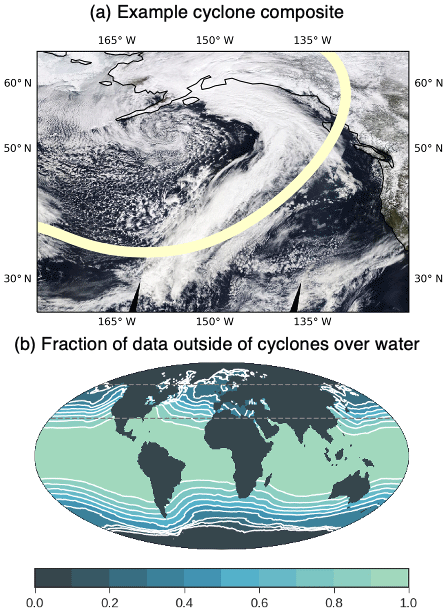
Figure 1(a) An example of a cyclone off the coast of North America from MODIS Aqua. The cyclone center has been identified south of the Aleut Peninsula based on MERRA-2 sea-level pressure (SLP). A line shows the edge of the area considered to lie within the cyclone following Field and Wood (2007). (b) The fraction of data outside of cyclones averaged between 2003 and 2015. The mean within the 30–60∘ N region is 42 %.
2.1 Region and variable selection
The empirical analysis on both observational and simulated data in this work follows pioneering studies investigating meteorological controls on subtropical (Myers and Norris, 2013, 2015; Qu et al., 2015; Klein et al., 2017; Seethala et al., 2015) and midlatitude (Miyamoto et al., 2018) marine boundary-layer cloudiness. The selection of variables used in this study is based on the findings of these earlier studies. The predictors examined here are sea surface temperature (SST), large-scale subsidence (ω) at 550 hPa, the strength of the inversion at the top of the boundary layer (estimated inversion strength – EIS – as defined in Wood and Bretherton, 2006), the total water vapor path (WVP), and sensible heat flux (SHF). A summary is given in Table 1. A priori we expect that increasing SSTs should lead to decreasing cloudiness (Myers and Norris, 2015; Qu et al., 2015; McCoy et al., 2017; Bretherton and Blossey, 2014). Increasing subsidence should decrease the liquid water path (Myers and Norris, 2013). Increasing inversion strength should lead to an increasing cloud fraction (Wood and Bretherton, 2006; Klein and Hartmann, 1993; Qu et al., 2015; Myers and Norris, 2015; Seethala et al., 2015). As shown in Miyamoto et al. (2018) from examination of midlatitude ocean fronts, increased SHF should increase cloudiness. Finally, while less extensively studied, an overall increase in WVP seems likely to lead to increased cloudiness as the atmospheric column moisture increases, holding all else equal (McCoy et al., 2019).

The central goal of this study is to develop an empirical constraint on aerosol–cloud adjustments. However, direct measurements of the aerosol state to constrain aerosol–cloud adjustments have been found to be sensitive to errors in pristine conditions (Ma et al., 2018). To develop a constraint on aerosol–cloud adjustments we examine the cloud microphysical state in addition to the meteorological parameters listed above. Cloud droplet number concentration is the state variable relating cloud macrophysics to aerosol concentration (Wood, 2012; Grosvenor et al., 2018) and is the predictor used in this study to characterize aerosol–cloud adjustments.
We hasten to note that the list of predictors described above is not intended to be complete (that is to say, we do not anticipate that we will be able to explain 100 % of the variability in clouds with these predictors). Our goal is to explain enough variability with these predictors to be able to infer statistically robust relationships between cloud macrophysical and microphysical properties in the variance unexplained by meteorological variability. The predictive ability of these inferred relationships will be tested within the context of a global climate model (GCM).
Having discussed predictors, we will now discuss predictands. Outside of cyclones cloud cover is primarily liquid, boundary-layer cloud, which substantially affects shortwave radiation but has little effect on longwave radiation (Hartmann and Short, 1980). Thus, we focus on the liquid water path (LWP) averaged over cloudy and clear regions. This variable allows observations and model output to be compared without needing to simulate output from a passive spectroradiometer (Bodas-Salcedo et al., 2011) or considering cloud overlap, as would be required for in-cloud LWP.
Analysis is carried out in the Northern Hemisphere (here 30–60∘ N) over oceans. This choice has been made for several reasons: first, there is a large variability in Nd across the northern midlatitudes that is not strongly driven by the seasonal cycle. In the Southern Ocean cloud condensation nuclei (CCN) variability is primarily due to biogenic sources, and their variability is strongly driven by the seasonal cycle, making analysis in the context of meteorological controls difficult to interpret (Ayers and Gras, 1991; McCoy et al., 2015a; Charlson et al., 1987). Second, Southern Ocean Nd is still poorly represented in the Met Office Unified Model GA7.1 (discussed in Sect. 2.4), with both too low a mean value and generally too small a seasonal cycle – in contrast to the Northern Hemisphere, which compares well with observations (Mulcahy et al., 2018).
2.2 Outside of cyclone compositing
The passage of synoptic systems is the central mode of variability in midlatitude cloudiness. McCoy et al. (2018b) focused on cyclone systems and showed that once meteorological variability was accounted for, the effects of changes in cloud microphysics driven by changes in Nd on liquid content are revealed. This work utilized the Field and Wood (2007) cyclone compositing algorithm, which uses sea-level pressure (SLP) to identify cyclone centers. Here we utilize the same compositing approach but focus on all data that are 2000 km away from a cyclone center, following Bodas-Salcedo et al. (2014). This separates the midlatitudes into times when a cyclone is nearby and when there is no cyclone nearby. Once cyclone centers are identified all data within 2000 km of an identified cyclone center are masked out of the data set. All data over land are also masked because microwave observations are unavailable (see next section).
A schematic representation of the frequency of occurrence of out-of-cyclone states is shown in Fig. 1b and is 42 % in the 30–60∘ N region focused on in this study. All data are regridded to a common 1∘ × 1∘ spatial resolution before analysis. All data are daily mean, except for observed Nd, which is only available for the MODIS Aqua overpass; however the diurnal cycle of Nd is thought to be relatively slight (Dong et al., 2014), and it is unlikely that this retrieval limitation significantly impacts our results. Our choice of resolution is motivated by the natural resolution of the Multisensor Advanced Climatology of Liquid Water Path (MAC-LWP) data set. Performing the analysis with a coarser resolution might change the regression coefficients derived in Sect. 2.5, as has been reported for analysis of the first indirect effect (McComiskey and Feingold, 2012). However, in Sect. 3.4 we validate the adjustments inferred from this resolution against the true adjustments in Met Office Unified Model (UM) GA7.1 (the atmosphere model of HadGEM3-GC3.1 and UKESM1) and find agreement, which demonstrates that our choice of resolution does not affect our results.
2.3 Observations
The cloud liquid water path (LWP) is calculated based on the aggregated observations from multiple satellite microwave sensors following the methodology of the multisensor advanced climatology of LWP (MAC-LWP; Elsaesser et al., 2017) at a daily mean resolution. Microwave radiometers are sensitive to total liquid. This means that the retrieval must calculate a partitioning between precipitating and non-precipitating liquid. Here, the liquid water path in clouds is calculated following Elsaesser et al. (2017). Previous analysis has shown that the midlatitude partitioning of rain and cloud in MAC-LWP compares favorably with convection-permitting simulations (McCoy et al., 2018b). The MAC-LWP data set estimates that 7 % of total liquid path is rain in the NH midlatitudes outside of cyclones. Because of the low fraction of rainwater in the midlatitudes outside of cyclones it is unlikely that the need to partition the observations into rain and cloud water substantially affects observational constraints as calculated in Sect. 3.3. The liquid water path is defined as the average of cloudy and clear regions and is insensitive to overlying ice cloud (unlike passive optical retrievals). This definition of LWP is consistent with the definition from GCMs. Microwave retrievals are only available over the ocean.
Observations of Nd are calculated based on MODIS observations of cloud optical depth and droplet effective radius. Level 2 swath data (joint product) from MODIS collection 5.1 (King et al., 2003) are filtered by removing pixels with solar zenith angles greater than 65∘ to eliminate problematic retrievals at a pixel level (Grosvenor and Wood, 2014). The daily mean Nd at 1∘ × 1∘ resolution is calculated from the filtered level 2 swath data and only low (cloud tops below 3.2 km), liquid clouds were used to calculate Nd. Only 1∘ × 1∘ regions where the liquid cloud fraction exceeds 80 % are considered valid (Bennartz et al., 2011), and the Nd is calculated using the effective radius from the 3.7 µm MODIS channel. This data set is evaluated in Grosvenor et al. (2018) and in McCoy et al. (2018a), where it shows consistency with measurements from aircraft.
We feel that this combination of radiometers in constraining adjustments is particularly advantageous because there is no shared information between the microwave retrieval of LWP and the shortwave and near-infrared retrieval of Nd. This is in contrast to the common practice of utilizing MODIS retrievals of cloud droplet effective radius and optical depth to calculate both the in-cloud LWP and Nd, making it conceptually difficult to cleanly infer changes in LWP due to changes in Nd.
The meteorological state of the atmosphere is characterized using reanalysis from MERRA-2 (Molod et al., 2015) and microwave observations of WVP from MAC-LWP. The period during which all of these observations are available stretches from 2003 to 2015. A list of variables and data sources is given in Table 1.
2.4 Simulations
Simulations are carried out in atmosphere-only simulations in the UM version 10.8 at N96 horizontal resolution. The version of the atmosphere model is GA7.1 coupled to the UKCA (UK Chemistry and Aerosols) model as described in (Mulcahy et al., 2018). The GA7.1 atmosphere model is the physical basis for the atmosphere model included in the HadGEM3-GC3.1 and UKESM1 climate model submission to CMIP6 (Walters et al., 2019). All simulations are run for 2 years and 3 months, starting in September 2013. Simulations are nudged to European Centre for Medium-Range Weather Forecasts (ECMWF) reanalysis winds above model level 16 (approximately 1.8 km). Paired simulations are conducted with emissions of aerosol and precursor gases set to preindustrial (henceforth labeled PI) and to present-day (labeled PD) levels. Anthropogenic emissions use the CMIP6 inventory (Eyring et al., 2016), natural emissions over land use the MEGAN-MACC inventory (Sindelarova et al., 2014), and natural emissions over the ocean follow the POET inventory (Granier et al., 2005). These simulations are conducted to calculate the response of cloud to anthropogenic aerosol. Additional sensitivity studies were carried out, starting with nudging at level 27 (approximately 5 km) and without nudging. In the latter case simulations of the PI and PD were run for 10 years and 3 months, starting in September 2003. The results of this analysis are shown in the Supplement and do not differ substantially from the results in the main text.
In GA7.1 aerosol number concentration has the potential to affect cloud microphysics in three places: first, the conversion of cloud water to rain, where enhanced Nd suppresses the conversion of cloud water to rainwater. This is parameterized using the scheme in Khairoutdinov and Kogan (2000), bias corrected as described in Boutle et al. (2014). The conversion rate of cloud to rain is parameterized as
where qCloud is the cloud liquid water mixing ratio. Second, it can affect cloud microphysics in the gravitational settling of cloud droplets, where enhanced Nd suppresses the settling of cloud droplets out of the cloud. The flux of water settling out of a cloud layer is given as
Third, it can affect cloud albedo through changes in Nd (Twomey, 1977).
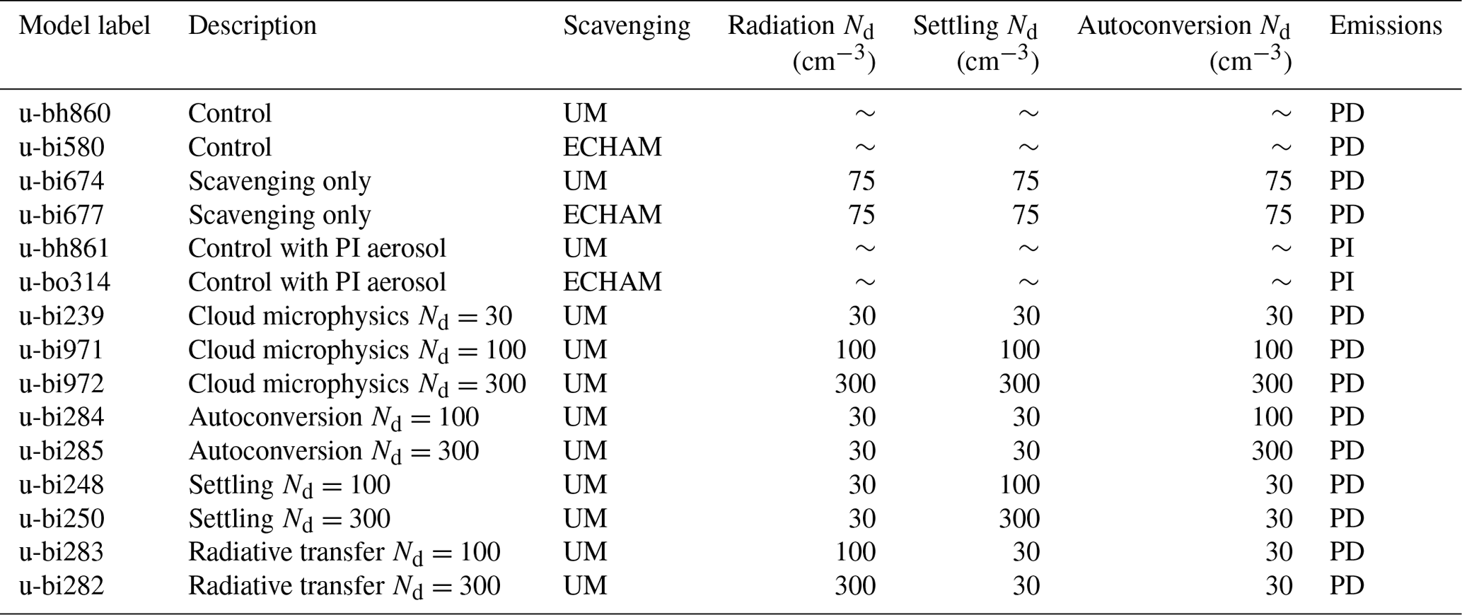
However, clouds may affect aerosol concentrations via wet scavenging. UKCA allows scavenging to be configured in two ways: the default configuration or using the scavenging coefficients in the ECHAM5-HAM model (Stier et al., 2005). To evaluate some of the uncertainty related to scavenging we perform simulations with both sets of coefficients. A list of model simulations conducted is given in Table 2.
Table 2List of simulations: the Met Office model designation; a short description; the scavenging coefficients used; the value of Nd used in the radiation, settling, and autoconversion parameterizations; and aerosol emissions period used (present day – PD – or preindustrial – PI). A tilde in Nd for a given parameterization indicates that Nd was not set to a constant value.
2.5 Analyzing covariance in the system
Our goal in this paper is to characterize how Nd drives LWP. However, to reveal robust correlations between Nd and LWP, meteorological variability must be accounted for. To achieve this we follow previous empirical analysis of cloud-controlling factors and utilize multiple linear regression to characterize the dependence of various cloud properties as predictands on the predictors described above (Myers and Norris, 2015). As with all empirical analyses of observations, correlation between predictors and the predictand does not necessarily mean that they are causally linked. The meteorological predictors selected here have had mechanisms hypothesized to link them to cloud variability. Another issue with this and similar analyses of the response of cloud to cloud-controlling factors is that thermodynamic and dynamical predictors within the Earth's atmosphere are correlated (McCoy et al., 2017; Myers and Norris, 2015, 2013). As the variance shared by predictors grows, the uncertainty in the coefficients calculated by multiple linear regression increases. While this is an issue, it is inescapable in trying to disentangle the effects of different cloud-controlling factors on cloud properties. Examples of meteorological variables that are correlated but have opposing effects on cloud cover include subsidence and stability and stability and SST (Myers and Norris, 2013; Qu et al., 2015; Wall et al., 2017).
To reduce predictor covariance we bin our 1∘ × 1∘ daily mean data from model output and observations into the space of SST and WVP. All output over oceans is considered in the analysis. We choose these predictors to bin our data before performing regression analysis because they represent two of the most basic meteorological state variables, because they covary strongly, and because LWP varies significantly as a function of WVP and SST in both observations and simulations (Fig. 2); 9 bins are used to span WVP (0–40 kg m−2), and 10 are used for SST (275–305 K). We propose that a multiple-linear-regression model of the form,
be trained in each bin of SST and WVP. All the predictors within the regression model are environmental drivers that are external to the clouds being influenced. However, robust remote-sensing observations of CCN are lacking and ln(Nd) is used in its place. As discussed above, Nd is predominantly a function of CCN availability. Thus, a multiple-linear-regression model,
is trained in each bin of WVP and SST. Bins that contain fewer than 3000 data points are excluded. (Units of LWP are in g m−2, Nd is in cm−3, subsidence is in Pa s−1, EIS is in K, WVP is in kg m−2, SST is in K, and SHF is in W m−2.) A 99 % confidence interval is used to determine if a coefficient is significant (different from zero). The initiation of precipitation in boundary-layer cloud can substantially impact LWP within a given cloud with a timescale longer than the daily sampling timescale utilized here (Berner et al., 2013). However, the spatial scale of our analysis (1∘ × 1∘) samples clouds at many stages of their life cycle. This means that we do not need to consider rain to be a predictor of LWP and may think of it as scaling with cloud LWP.
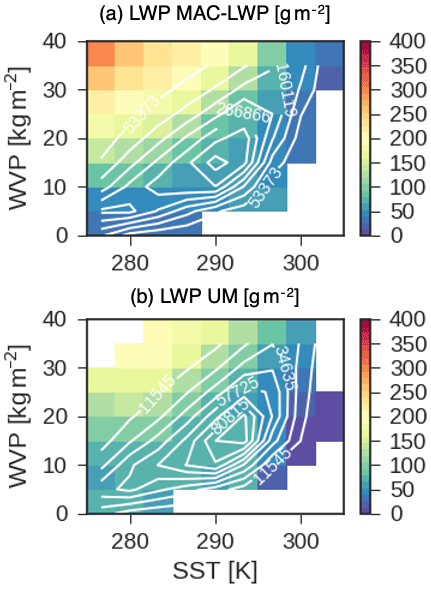
Figure 2MAC-LWP-observed (a) and UM-simulated (b) LWP in the space of SST and WVP in the region 30–60∘ N. White lines show the distribution of data in SST–WVP space. The contours of number of observations in each bin are shown in white.
Training the regression model in Eq. (4) produces a measure of the covariance between predictors and predictands. In particular, it produces a measure of the covariability between ln (Nd) and LWP (a1). However, this covariance does not show causality. Nd may enhance LWP by, for instance, suppressing rain (Albrecht, 1989), and it is this relationship where causality runs from Nd to LWP that is of interest in understanding adjustments. However, the observed covariability between Nd and LWP is also the product of causality running from LWP to Nd due to precipitation removing aerosol and reducing Nd (Wood et al., 2012). The overall covariance between Nd and LWP is the product of these two causal pathways as well as correlation induced by environmental factors driving both clouds and aerosol and by geographic and seasonal distribution of sources of aerosol relative to cloud. Figure 3 shows a schematic of these causal flows.
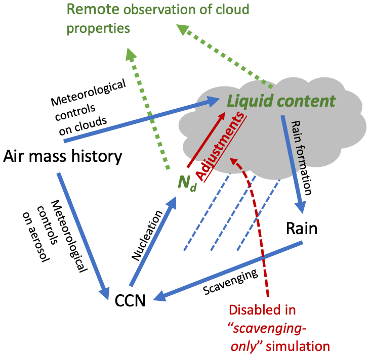
Figure 3A schematic illustration of the mechanisms linking cloud, aerosol, and meteorology considered in this study. Observed quantities are shown in green (in this case Nd and LWP). Adjustments (shown in red) are the causal link that flow from Nd to LWP, and inferring them is the focus of this study. In the “scavenging-only” simulation the Nd seen by the cloud physics is set to a constant value.
How do we constrain adjustments based on examination of modeled and observed Nd and LWP if we cannot disentangle causality? The solution we propose is to use a simplified version of the model to characterize the sensitivity of Nd to precipitation and other factors and use this sensitivity to interpret the full model. To conceptualize why this process can estimate the sensitivity of LWP to Nd we can write an equation describing small changes in LWP in the space of small changes in Nd. First, we consider that Nd acting on cloud microphysics () and Nd when precipitation scavenging is the only causal factor linking cloudiness and Nd () as separate entities. In the latter case air mass history and sinks unrelated to precipitation can affect Nd, in addition to the effect of precipitation scavenging, but precipitation scavenging is the only causal link between cloud and aerosol (see Fig. 3). We consider changes in LWP relative to and . That is to say we consider , where the logs are added for consistency with Eq. (4) and all other terms in Eq. (1) are held fixed and the first term is expanded.
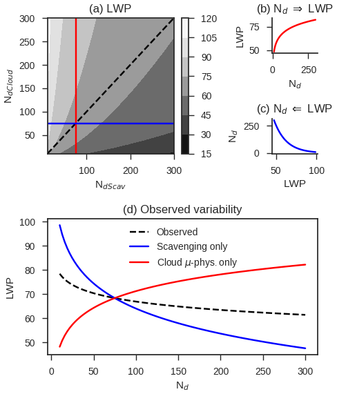
Figure 4A simple conceptual model demonstrating how variance due to precipitation driving of Nd and due to Nd driving changes in LWP through cloud microphysics affects total covariance between Nd and LWP in observations and models. Nd where scavenging is the only causal link between cloud and aerosol (NdScav) and Nd affecting the cloud microphysics (NdCloud) are considered to be distinct entities. The contour map in (a) illustrates a potential topological LWP space in terms of NdCloud and NdScav. The case where NdCloud is set to a constant value is shown with a blue line, and the case where NdCloud is increased independently is shown with a red line. In a causal sense this implies NdCloud driving LWP (shown in b) and NdScav being driven by LWP (shown in c), where NdScav is negatively correlated with LWP because and , where R is rain rate. The observed variability in LWP in terms of Nd is shown in (d) for the cases NdCloud=Nd and NdScav=constant (red), NdScav=Nd and NdCloud=constant (blue), and (the real world; dashed line).
Conceptually, LWP is increased with increasing (Fig. 4b), and is reduced by increasing rain rates, which increase with LWP (Fig. 4c). In the topographic space describing LWP in terms of and , reduced corresponds to increased precipitation rates and, in turn, LWP. That is to say,
where R is the rain rate, so the reciprocal of the product of these terms gives
Thus, a small change in LWP in terms of changes in these two variables alone is
We assume that scavenging is unaffected by changes in affecting rain rates, so there are no higher-order terms, although this may not be the case in reality (Wood et al., 2012), and this feedback is found to substantially enhance the strength of adjustments in some models (Jing and Suzuki, 2018). A visualization of Eq. (7) is shown in Fig. 4a. The best fit of LWP to Nd gives the sum of the partial derivatives of the two terms
where subscripts on the partial derivatives indicate that they are evaluated while holding that variable constant. In the control simulation, because NdCloud and NdScav are not distinct entities. That is to say, the cloud microphysics and radiation see that the Nd calculated by the nucleation scheme and aerosol experiences the effects of scavenging and meteorology. In this particular case the derivatives of and each go to unity because the Nd seen by the cloud and affected by scavenging is equal, and we are left with
We always sample along the dashed line in Fig. 4a in the observational record or in a model where clouds are sensitive to Nd and aerosol is scavenged, giving the curve in Fig. 4d. This curve combines the effects of causality flowing from Nd to LWP and from LWP to precipitation to aerosol and onto Nd. The term is the key to constraining adjustments because it describes the sensitivity of LWP to changes in Nd (in this analogy the slope of LWP along the red line in Fig. 4a). While we cannot disentangle causality in observations or in a model where Nd affects cloud microphysics, we propose that in a model configuration where cloud microphysics (e.g., radiation, settling, and autoconversion in UM GA7.1) are unaffected by Nd we may estimate the term . That is to say, if and , then
and the best fit of LWP to Nd in the scavenging-only simulation is just a measure of the scavenging of aerosol by precipitation and the non-causal covariance between Nd and LWP induced by other confounding factors.
Thus, the sensitivity can be estimated as the difference between the regression of LWP on Nd trained in a simulation where clouds are insensitive to Nd (; scavenging only) and the regression in a control simulation () because
We will use this correction for variability induced by factors besides adjustments throughout the paper to infer the effects of Nd on cloud properties in model configurations and the observations. We note that this methodology is subject to several limitations. First, as noted above, it assumes that feedbacks between adjustments and scavenging are small. This assumption will break down as adjustments become stronger. However, the response in cloud to transient changes in aerosol does not appear to permit very strong adjustments (Malavelle et al., 2017; Toll et al., 2017, 2019). Second, it is assumed here that the relationship between LWP and ln (Nd) is linear. Empirically this assumption appears to hold in the models and observations (as shown in the following section), and inclusion of higher-order polynomials of ln (Nd) in Eq. (3) did not alter our results.
To reiterate, non-causal factors also lead to correlation between Nd and LWP because air mass history is important for both clouds and aerosol (Mauger and Norris, 2007). In the discussion of the conceptual model presented above we focused on the impact of changes in Nd on LWP and vice versa. Spurious correlation due to air mass history will affect both terms on the right-hand side of Eq. (11) when they are calculated using regression. Thus, the correction for scavenging-induced variability in Eq. (11) also corrects for variability induced by air mass history simultaneously affecting Nd and LWP.
3.1 Variance in LWP as a function of Nd
As described in the Methods section, data from observations and the control simulation in the UM between 30 and 60∘ N over oceans and 2000 km from cyclone centers at a daily mean resolution are binned by WVP and SST, and the regression model shown in Eq. (4) is trained in each bin. If we plot the quantity,
as a function of Nd we can see that the coefficient relating LWP to Nd is greater than zero at 99 % confidence, once variability associated with meteorological predictors is removed (Fig. 5). The residual variance in LWP covaries with Nd similarly between the observations and UM simulations where observations exist. However, one key difference is the span of Nd values in the observations and simulations. Observed Nd almost never falls below 30 cm−3 (the grey line in Fig. 5), while the Nd calculated by the model occasionally falls below this value (∼ 10 % of modeled ln (Nd)). This is not surprising because the model suffers from no retrieval limitations and can always measure an Nd, even when cloud is extremely tenuous. Ultimately the goal of this study is to utilize the slope of LWP with respect to Nd to infer adjustment strength. However, using the slope from the observations and the models will produce quite different values due to the strong increase in LWP with Nd below 30 cm−3. In order to compare observations and models fairly we exclude data for .
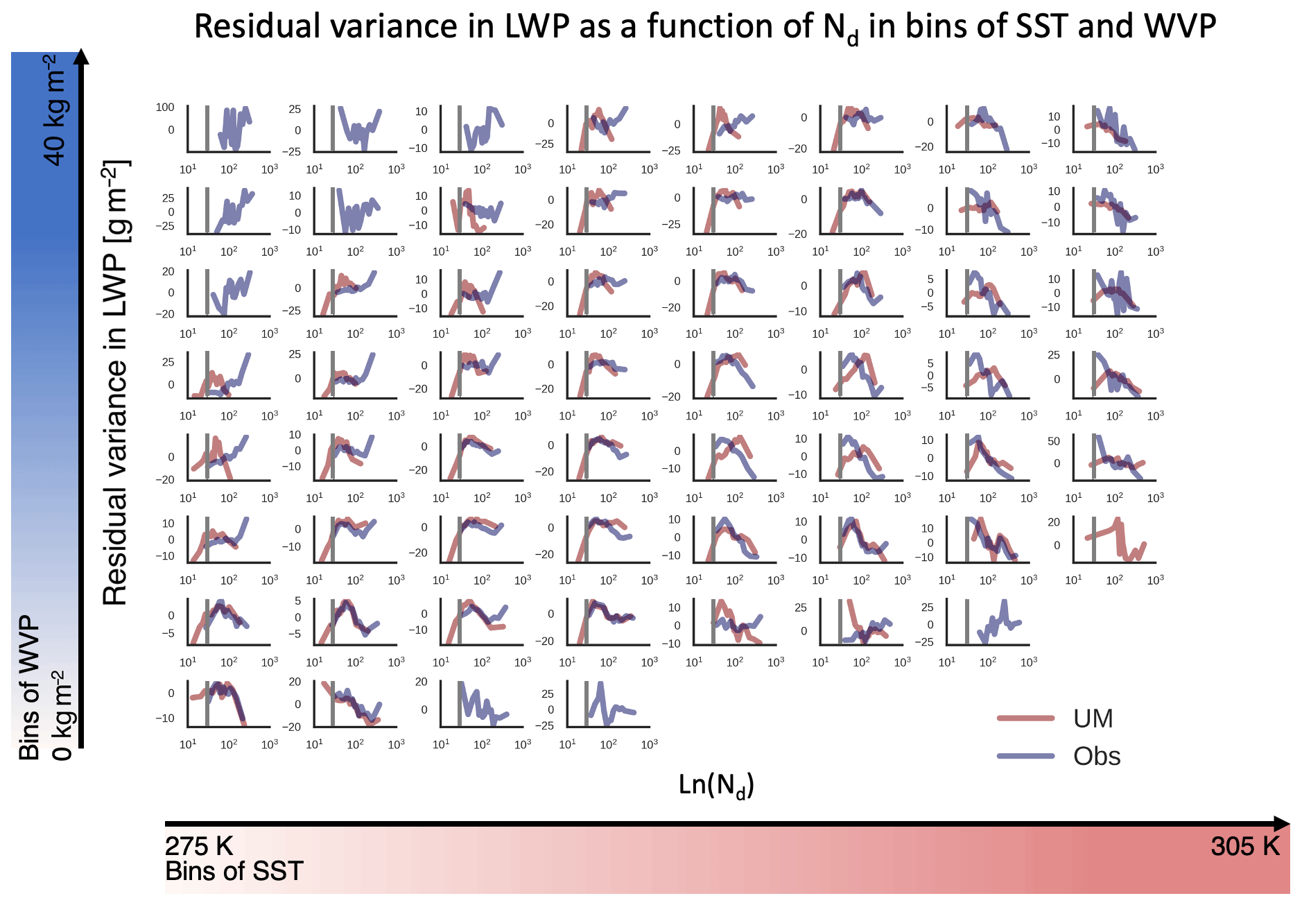
Figure 5Residual variance in LWP after removing variability associated with other predictors (Eq. 12) plotted as a function of Nd in the UM GA7.1 and observations (Obs.). Each subplot corresponds to a bin of WVP and SST. Due to retrieval limitations, values of Nd below 30 cm−3 (grey line) are almost never observed but occur in model output.
For residual LWP decreases with increasing Nd in both observations and models. This agrees with the notion that precipitation variability drives Nd (Wood et al., 2012) and agrees with previous analysis (Gryspeerdt et al., 2019). Clearly, this does not mean that the model reduces cloudiness in response to aerosol. The cloud microphysics within the UM GA7.1 must increase LWP in response to a change in Nd, and analysis of the model response to changes from preindustrial (PI) to present-day (PD) aerosol confirmed a negative forcing from adjustments (Mulcahy et al., 2018). As discussed in the Methods section, the difference in slopes between the scavenging-only and control simulation is a proxy for the response in cloud microphysics to Nd. Before analyzing this difference, we will briefly discuss the covariance between LWP and meteorological predictors in the observations and the control simulations.
3.2 Covariances between LWP and meteorology
Before returning to discussing aerosol–cloud adjustments, we discuss the covariances between observed LWP and the other predictors in Eq. (4). This is shown in Fig. 6. The explained variance (R2) by the regression model exceeds 40 % except at low WVP and SST. The variance explained across all bins of SST and WVP is 46 % of daily mean 1∘ × 1∘ variability. That is to say, nearly half of the day-to-day variability in LWP across the midlatitudes away from cyclones can be explained as a simple linear combination of five variables.
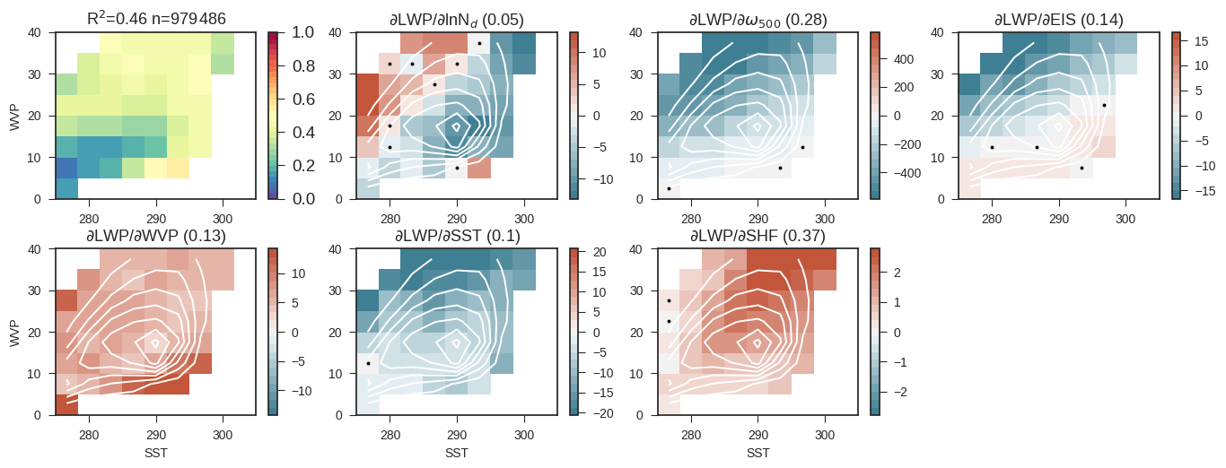
Figure 6The regression coefficients relating observed LWP to predictors in the phase space of SST and WVP. Regression coefficients not significant at 99 % confidence are marked with a dot. White contours show the distribution of observations in the WVP–SST phase space. The first plot shows the explained variance in each bin. The explained variance within the entire data set is noted in the title along with the number of observations. The remaining plots show the coefficients relating each predictor to LWP. In the title the weighted mean of the absolute value of the standardized coefficient ( is shown in brackets to give an estimate of contribution of each predictor to the variance. Regression coefficients are as described in Eq. (4).
Several of the predictors have uniform effects on LWP: LWP decreases with subsidence (consistent with Myers and Norris, 2013), increases with WVP, decreases with increasing SST (consistent with Qu et al., 2015, and references therein), and increases with sensible heat flux (consistent with Miyamoto et al., 2018). We note that at very low SST it appears that LWP may increase with SST. It is possible that this feature is related to ice-to-liquid transitions (McCoy et al., 2015b, 2016; Tsushima et al., 2006; Senior and Mitchell, 1993; Tan et al., 2016), but this region only accounts for a small fraction of the overall data volume. The only meteorological predictor that correlates positively and negatively with LWP across the SST–WVP phase space is EIS. At higher WVP and lower SST, EIS and LWP are negatively correlated, while at low WVP and high SST, they are positively correlated. The latter effect is consistent with increasing EIS increasing the cloud fraction (Wood and Bretherton, 2006). One possibility is that because clouds are closer to 100 % in areal coverage at higher WVP and lower SST, increasing stability suppresses the thickening of cloud in this regime, while the clouds cannot expand horizontally.
Examination of the control simulation shows very similar covariances between meteorological predictors and LWP (Fig. 7). Notable differences are the stronger positive covariance between SST and LWP at low SST and uniform negative covariance between EIS and LWP across the SST–WVP phase space. However, the relationship between LWP and meteorology is strikingly similar to that between observations and the UM. The explained variance by predictors tends to be higher in the UM GA7.1 (64 %), but it is hard to say how much of this difference in explained variance is due to simplification of the real atmosphere and cloud physics by the model and how much is due to observational error.
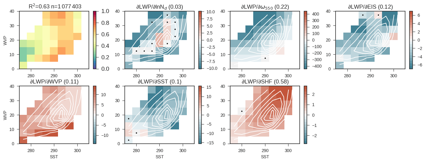
In this framework we also characterize the covariance between ln (Nd) and LWP. The correlation between ln (Nd) and LWP is primarily negative in the observations, with positive correlations only occurring at high WVP and low SST. The correlation between LWP and ln (Nd) in the model is almost uniformly negative (in the data set restricted to ). Standardization of the predictor strength estimates the effect of a standard deviation change in each predictor in standard deviations of LWP. In both the observations and models the impact of a standard deviation in meteorological predictors dwarfs the effect of a standard deviation in ln (Nd), with contributions from subsidence and SHF dominating variability. That is to say, the relative contributions of variability in Nd are quite small in comparison to variability that is simply due to the weather.
3.3 Inferring the effect of Nd on LWP
As we have seen, the correlation between LWP and Nd is mostly negative. The slope relating ln (Nd) to LWP in the context of Eq. (4) is reproduced in Fig. 8a and b. However, if we manually set the Nd seen by autoconversion, radiation, and settling to 75 cm−3 in the UM GA7.1 (the approximate mean value in the study region) the negative covariance strengthens substantially (Fig. 8c). This model version is termed “scavenging only” because scavenging is the only causal link between cloud and aerosol (Fig. 3). As discussed in the Methods section, the effect of changes in Nd on LWP may be approximated by the difference between Fig. 8b and c. This is shown in Fig. 8e. This agrees with our expectation based on our knowledge of how the UM GA7.1 treats liquid cloud processes. We know that the effect of increasing Nd on autoconversion and settling is to inhibit the conversion of cloud to rain and reduce cloud droplet fall speed.
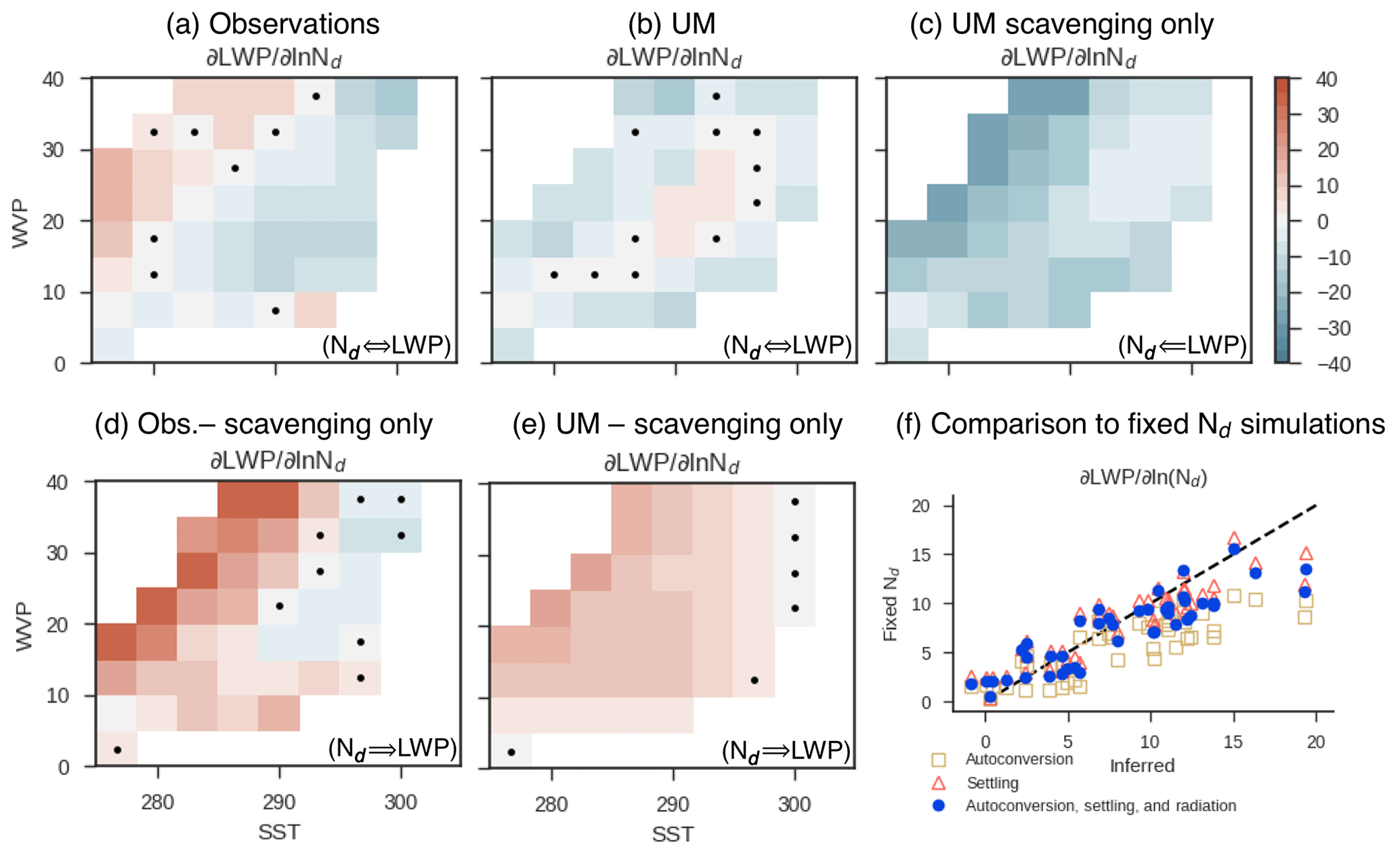
Figure 8The observed covariance between Nd and LWP and the inferred effect of Nd on LWP. Notations in the bottom right of plots indicate the expected direction of causality. The covariance between Nd and LWP is shown in (a) the observational record (as in Fig. 6) and (b) the control simulation of the UM GA7.1 (as in Fig. 7); (c) a simulation where the Nd seen by the autoconversion, settling, and radiation is set to 75 cm−3 and only scavenging links Nd and LWP. The inferred strength of adjustments in observations (d) calculated as the difference in slope between (a) and (c) as in Eq. (11), and in (e) the UM is calculated as the difference in slope between (b) and (c). Inferred and true adjustment strength for the UM is compared in (f). The inferred adjustment strength in (e) is compared to the sensitivity of LWP to Nd in a set of simulations where Nd is fixed in the autoconversion, settling, and radiation to a range of values, forcing causality to flow from Nd to LWP. The 1 : 1 line is shown with dashes. Different symbols indicate whether the Nd seen by the autoconversion, settling, or radiation was varied while others were held constant. Each symbol corresponds to a bin in WVP and SST, as in (e).
To evaluate the accuracy of this method in inferring the sensitivity of LWP to Nd we conduct simulations where causality is forced to flow from the Nd to LWP. This is done by setting the Nd seen by the autoconversion, settling, and radiation to constant values. Two simulations are conducted for each mechanism, with Nd set to 100 and 300 cm−3. The Nd seen by the other mechanisms is held constant at 30 cm−3. A further three simulations are conducted, in which Nd seen by all three mechanisms is set to 30, 100, and 300 cm−3 (Table 2). This yields a set of simulations describing the effects on LWP of an increase in Nd in the autoconversion, settling, or radiation as well as via all three mechanisms simultaneously. Analysis of the effects of increased Nd seen by the radiation code showed negligible changes in LWP and is not shown here.
As in Fig. 7, the fit in Eq. (4) is trained in each bin of WVP and SST across each set of three simulations. The Nd seen by the model parameterization is used in the multiple linear regression (Eq. 4). As expected, given the functional form of these parameterizations (Eqs. 1 and 2) the effect of increasing Nd in either autoconversion or settling results in an increase in LWP, as does the case where Nd in the settling, autoconversion, and radiation are all varied together. The effect of a perturbation in the Nd seen by autoconversion, radiation, and settling on LWP is nearly identical to the slope inferred by subtracting the slope in the scavenging-only run from the control run following Eq. (11) (Fig. 8f). This comparison between the true model sensitivity of LWP to changes in Nd supports the validity of the multiple-linear-regression-based inference approach pursued here.
Autoconversion and settling are likely to interact with each other in a non-linear manner. As one is suppressed as a sink of cloud liquid, the other will grow (for example, if the conversion of cloud to rain is rendered inefficient, then the gravitational settling of cloud droplets will become more efficient as the liquid content grows). Analysis of crosstalk between these terms is not the focus of this article, but sensitivity of LWP to changes in each mechanism is shown in Fig. 8f. The effect of perturbing settling Nd on LWP is larger than the effect of perturbing the autoconversion Nd, singling it out as an important lever in controlling adjustment strength for future study. This result is consistent with the large process rate for settling relative to autoconversion found in weakly precipitating low-cloud regimes in CAM5 (Gettelman et al., 2013). It is also possible that interactions between settling and Nd may decrease the sensitivity of warm rain to autoconversion representation that is diagnosed in other models (Michibata et al., 2019; Jing et al., 2019). Overall, the results of this study are insensitive to whether settling or autoconversion has a stronger effect on aerosol–cloud adjustments because we assume that feedbacks between scavenging and adjustments are small.
Given that the scavenging-only simulation can be used to infer the adjustment strength in the UM, we also attempt to use the scavenging-only simulation to infer the strength of adjustments in the real world (Fig. 8d). This assumes that the statistical relationship between LWP and rain rates in the UM GA7.1 and the scavenging of CCN-relevant aerosol by precipitation in the UM GA7.1 is realistic.
Based on the covariance between Nd and LWP in the scavenging-only simulations in the UM GA7.1 and observations we offer an estimate of adjustment strength. The adjustment strength inferred from observations is stronger than the UM for low SST and high WVP. Unlike the UM, weak negative covariance between LWP and Nd exists for high SST and low WVP. This may indicate that the scavenging of aerosol by the UM is too efficient, or some other confounder of the relationship between LWP and Nd is poorly represented in the model, or it may point to the thinning of cloud via enhanced entrainment (Ackerman et al., 2004), which is not represented in the UM. Overall, the effect of increasing Nd in the UM is an increase in LWP.
We have discussed how to infer adjustment strength from the total covariance between Nd and LWP, which mixes covariance induced by causality flowing from cloud to aerosol and aerosol to cloud. In the next section we show how this inferred adjustment strength from the simple regression model is able to predict LWP adjustments in response to anthropogenic aerosols within the full GCM simulation.
3.4 Reproducing simulated adjustments between the preindustrial and present-day aerosol emission
We have produced an estimate of the sensitivity of LWP to changes in Nd in the UM GA7.1 model (Fig. 8e). Does this simple regression model hold skill in reproducing the actual change in LWP within the model between the present-day (PD) and preindustrial (PI) aerosol emissions? Simulations are carried out by setting aerosol emission to preindustrial values. This is done for simulations using the GA7.1 scavenging parameterization. A second set of simulations is conducted where the ECHAM-HAM5 scavenging coefficients are used to estimate the sensitivity to the representation of scavenging. PI, PD, and scavenging-only simulations are conducted for each scavenging configuration.
The change in LWP between the PI and PD (ΔLWPPD−PI) simulated by the UM is 2.9 g m−2, averaged across the 30–60∘ N region. Using the UM-simulated change in Nd (ΔNdPD−PI) and the slope relating ln (Nd) to LWP diagnosed from present-day variability (Fig. 8) we calculate ΔLWPPD−PI. If the covariance between ln (Nd) and LWP observed in the control run (Fig. 8b) of the model and ΔNdPD−PI is used to predict ΔLWPPD−PI, the negative correlation introduced by precipitation scavenging leads to a negative ΔLWPPD−PI (Fig. 9a; in disagreement with the UM-simulated ΔLWPPD−PI). If the covariance in the scavenging-only simulation (causality flows from clouds to precipitation to aerosol to Nd) is used (Fig. 8c), the regression-model-predicted decrease in LWP between PI and PD aerosol levels doubles. However, if we subtract the sensitivity in scavenging-only simulation from the control simulation to yield the sensitivity of LWP to changes in Nd (Fig. 8e), the ΔLWPPD−PI predicted by the regression model and the UM-simulated ΔNdPD−PI agree well with the UM-simulated ΔLWPPD−PI (Fig. 9). This result supports the utility of the inferred sensitivity of LWP to Nd in examining adjustments due to PD aerosol.
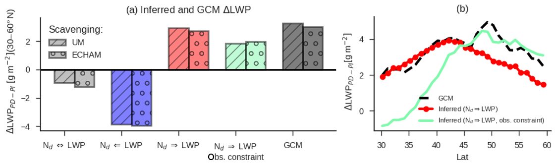
Figure 9The change in LWP between the simulations with PI and PD aerosol emissions (ΔLWPPD−PI) inferred by covariance between Nd and LWP in the PD and as simulated by the UM. The inferred ΔLWPPD−PI is calculated using the UM-simulated change in Nd. Panel (a) shows the inferred ΔLWPPD−PI based on variance in different simulations. The direction of causality is indicated for each case. From left to right: ΔLWPPD−PI inferred from covariance in the control simulation (Nd⇔LWP, causality between Nd and LWP goes both directions; Fig. 8b), inferred from the scavenging-only simulation (Nd⇐LWP, causality from LWP to Nd; Fig. 8c), inferred by correcting the total covariance using covariance in the scavenging-only simulation (Nd⇒LWP, causality goes from Nd to LWP Fig. 8d – this is the adjustment strength in UM GA7.1 inferred by the method presented in this paper) and when the covariance in observations is combined with the scavenging-only simulation (listed as Obs. constraint). The ΔLWPPD−PI simulated by the GCM is shown on the right in black. This is the true aerosol–cloud adjustment in the GCM that is compared to the value being inferred in the UM GA7.1, as shown by the red bars. ΔLWPPD−PI is provided for simulations using the UM GA7.1 scavenging coefficients and ECHAM-HAM5 scavenging coefficients. Panel (b) as in (a) but resolved in latitude and only showing the case when the UM GA7.1 default scavenging is used.
What does the covariance between LWP and ln (Nd) in the real world tell us about the model? Use of the observational estimate of adjustment strength (Fig. 8d) calculates a ΔLWPPD−PI that is two-thirds of the ΔLWPPD−PI inferred from the control run and ΔNdPD−PI (Fig. 9). This is because, while the inferred sensitivity of LWP to Nd from observations is quite strong in some regions, it is weakly negative in the most commonly occurring WVP–SST regimes (Fig. 8d). That is to say, if the efficacy of precipitation in removing CCN-relevant aerosol in the real atmosphere is near to the efficacy in the UM, the relationship between LWP and rain rates in the real atmosphere is near to the relationship in the UM, and the covariability between Nd and LWP induced by other confounders of the Nd–LWP relationship is realistic, then the adjustments (ΔLWPPD−PI) simulated by the UM are not unreasonable, albeit a little large. This result is consistent with constraints provided by simulation of the Holuhraun eruption (Malavelle et al., 2017), which showed that the anomaly predicted by HadGEM3 was within the observed range. However, the observationally inferred sensitivity of LWP to changes in Nd is stronger in low-SST and high-WVP regimes than it is in the UM GA7.1 but much weaker, or even slightly negative, in low-WVP and high-SST regimes. This results in a strong latitudinal gradient in ΔLWPPD−PI between 30 and 60∘ N inferred from observations (Fig. 9b).
The predicted ΔLWPPD−PI based on the control and scavenging-only simulations (Fig. 8e) underestimates the UM-simulated ΔLWPPD−PI by around 10 %. This may result from disregarding feedbacks between precipitation suppression and Nd (Jing and Suzuki, 2018), may simply be due to shortcomings in the simple linear model relating ln (Nd) to LWP, or may relate to meteorological differences between the PI and PD simulations not accounted for by meteorological predictors or compositing. However, the fractional reduction in inferred ΔLWPPD−PI when observations are used to constrain the sensitivity of LWP to Nd suggests that ΔLWPPD−PI should be around 60 %–70 % of the value predicted by the UM GA7.1 averaged across the NH. ΔLWPPD−PI inferred from observations is extremely dependent on latitude, with almost no change in LWP over lower latitudes and warmer SSTs. We hasten to note that the change in Nd between the PI and PD is uncertain and its prediction by UM GA7.1 may be biased, making the absolute values of the constrained ΔLWPPD−PI less relevant than the fractional overestimation in UM-simulated ΔLWPPD−PI. This analysis is repeated using simulations that are only nudged above level 27 of the model (Fig. S1) and not nudged at all (Fig. S2), with minimal differences from the results presented in the main text.
We have focused on changes in LWP in this work because it is a variable that we have good observations of, it can be compared between models and observations in a straightforward way, and it clearly links to adjustments. However, this variable is not the key variable in discussing radiative forcing and climate sensitivity. How does the radiative forcing from adjustments scale with LWP? Determining the precise effects of adjustments on the shortwave cloud radiative effect is difficult, but if we assume that the perturbations in LWP induced by adjustments are similar to the perturbations that are driven by meteorology, we can offer a simple estimate to inform our understanding of the modeled forcing from adjustments.
Examination of the relationship between LWP and albedo within the UM GA7.1 shows a rapid climb in albedo for low LWP, followed by saturation at higher values, as expected from saturation of the cloud fraction and optical depth (Fig. 10). This curve can be fit by a second-degree polynomial, meaning that the sensitivity of albedo to changes in LWP is a function of the LWP. That is to say, regions where LWP is already high are going to have a smaller increase in albedo for a unit change in LWP. The change in LWP between PI and PD is much smaller than the range of the variation in LWP in the climate mean state, so we use the average of monthly mean LWP between PI and PD to calculate the sensitivity of albedo to changes in LWP for the NH midlatitudes. This sensitivity (dα∕dLWP) is multiplied by the change in LWP to yield change in albedo. This change in albedo is scaled by the downwelling shortwave to give the change in reflected shortwave.
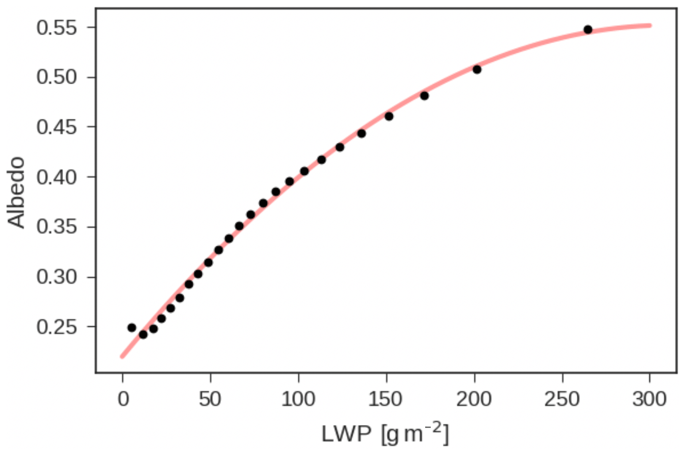
Figure 10UM GA7.1 daily mean albedo as a function of LWP over ocean between 30 and 60∘ N and outside of cyclones in equal quantiles of LWP (black circles). A second-order polynomial fit is shown using a red line.
The change in reflected shortwave predicted from LWP changes in the UM GA7.1 is 1.9–2.0 W m−2, depending on the scavenging parametrization used. The change in shortwave inferred from the regression model of LWP trained in the control run and corrected by the scavenging-only run is 1.5 W m−2. If the observed sensitivity of LWP to Nd is used to constrain ΔLWP, the predicted change in reflected shortwave is approximately 1.0 W m−2. Thus, we estimate that GA7.1 overpredicts the change in reflected shortwave due to adjustments in response to a given change in Nd by around 50 %. This estimate is subject to the caveat that changes in LWP due to adjustments may not affect albedo in the same way as suggested by examining the total variability. For example, adjustments might only increase the liquid content of the thickest clouds and have a relatively slight impact on albedo. However, it is unclear how to provide a more complex calculation than the one presented here.
As the possible range for the radiative forcing from the first indirect effect has narrowed, aerosol–cloud adjustments have become an increasingly central source of uncertainty in aerosol–cloud radiative forcing (Bellouin et al., 2020). Here we focus on the northern midlatitudes, where the majority of anthropogenic aerosol is emitted (Myhre et al., 2013). Previous work has examined aerosol–cloud adjustments in midlatitude cyclones, showing that cyclone liquid water path (LWP) increases with cloud droplet number concentration (Nd; McCoy et al., 2018b). This work focuses on the remainder of cases in the midlatitudes, when there is no cyclone center within 2000 km (roughly 42 % of the time between 30 and 60∘ N; see Fig. 1).
Untangling the effect of cloud microphysics on cloud macrophysics from the total variability in cloud macrophysics is challenging. In the observational record we can only characterize the covariance between predictors and predictands. In interrogating the observed covariances between cloud properties and different meteorological predictors we find many of the relationships that have been described in the literature documenting cloud-controlling factors (Myers and Norris, 2015). Once meteorological variability is accounted for, statistically significant relationships between cloud microphysics (Nd) and cloud macrophysics (LWP) appear. In keeping with previous studies (Gryspeerdt et al., 2019), LWP and Nd are found to be negatively correlated. However, this is clearly not consistent with the UM GA7.1 GCM's actual response in LWP to changes in aerosol emissions between PI and PD. This negative correlation is due to a combination of Nd being driven by scavenging, as shown in Wood et al. (2012), and spurious correlation between Nd and LWP driven by external variables affecting both terms (Mauger and Norris, 2007), overwhelming any positive covariance driven by aerosol–cloud adjustments.
While we cannot disentangle the covariance due to adjustments and covariance due to scavenging and other confounders in the observational record, we can create simulations in which causality is forced to flow from clouds to Nd (scavenging only). Using this measure of non-adjustment-induced variability in Nd, we can infer the effect of changing Nd on LWP. This inferred sensitivity of LWP to Nd agrees well with simulations where Nd is manually varied in the cloud microphysics (Fig. 8f). The inferred sensitivity of LWP to Nd, combined with the UM-predicted change in Nd, reproduces the UM-predicted change in LWP between the PI and PD (ΔLWPPD−PI; Fig. 9). These two tests support this method's relevance to understanding aerosol–cloud adjustments.
The analysis presented here, combined with the enhancement in LWP in cyclone systems shown in McCoy et al. (2018b), points toward an overall increase in LWP across the NH midlatitudes in response to anthropogenic aerosol. Ultimately, while the regimes examined here and in McCoy et al. (2018b) are very different, the detection of a change in LWP in response to changes in Nd rests on the ability of the technique to account for non-adjustment-induced variability in Nd. In McCoy et al. (2018b) this was done by stratifying the data set by the cyclone precipitation rate, which is well-constrained by the large-scale environment (Field and Wood, 2007); this in turn stratifies the data set by the scavenging of aerosol.
Assuming that scavenging in the UM GA7.1 model is realistic, that the relationship between LWP and precipitation is reasonable, and that the non-causal covariance produced by other factors is replicated in the model, we evaluate the strength of adjustments based on observations. This reveals that the present version of the UM GA7.1 overestimates the sensitivity of LWP to changes in Nd by approximately 50 % outside of midlatitude cyclones. Calculation of the implied change in shortwave shows a similar overestimate in forcing due to adjustments by the UM. Observations also imply that aerosol–cloud adjustments in the UM GA7.1 occur in the wrong regime. Adjustments in the UM favor warmer SSTs and lower WVP, while the observations favor colder SSTs and higher WVP. This difference in regime may be due to early precipitation onset in the UM GA7.1.
The present study and McCoy et al. (2018b) project a negative forcing due to adjustments in the midlatitudes. Extension of this study to the subtropics and tropics is reserved for a future analysis. While extrapolating the present results to the tropics is difficult, it seems reasonable to suppose that the pattern of adjustments in the subtropics is relatively similar to the inter-cyclone regime analyzed here and to expect a negative forcing in this region due to adjustments, although this may be weaker than the midlatitude adjustments due to decreasing LWP for increasing Nd over higher SSTs and lower WVP over some of the subtropics (Fig. 8d). One important limitation of this study is that it assumes weak feedbacks between adjustments and scavenging. If some regimes have very strong feedback between precipitation and adjustments, then our analysis will infer adjustments that are too weak.
Our result is in contradiction with previous empirical constraint studies that have postulated that changes in Nd greatly enhance LWP (Rosenfeld et al., 2019), have little effect (Malavelle et al., 2017; Toll et al., 2017), or reduce LWP (Sato et al., 2018; Gryspeerdt et al., 2019). We suggest that this diversity within the literature is because a range of constraints may be arrived at, depending on the degree to which precipitation scavenging and meteorological driving of aerosol and cloud occludes aerosol–cloud adjustments and the steps that are taken in the analysis to account for scavenging-induced and meteorologically induced covariability. Based on the analysis presented here we believe that positive, zero, or extremely strongly negative radiative forcings due to aerosol–cloud adjustments in the midlatitudes are not supported by the observations.
MERRA-2 data were downloaded from the Giovanni data server (https://disc.gsfc.nasa.gov/datasets/M2T1NXSLV_V5.12.4/summary?keywords=merra-2; last access: 22 July 2019; Global Modeling and Assimilation Office, 2015). CERES data were downloaded through the ordering interface at https://ceres.larc.nasa.gov/order_data.php (last access: 22 July 2019) (Doelling et al., 2019).
The supplement related to this article is available online at: https://doi.org/10.5194/acp-20-4085-2020-supplement.
All authors contributed ideas and helped with editing the paper. DTM and PF planned the paper. Data analysis and writing were undertaken by DTM. Present-day and preindustrial simulation suites were set up by HG. Simulations were run by DTM. Idealized simulations were set up by DTM. Development of simulations was conducted by HG, PF, DPG, and DTM. MODIS data were created by DPG. MAC-LWP data were created by GSE.
The authors declare that they have no conflict of interest.
We acknowledge use of the MONSooN system, a collaborative facility supplied under the Joint Weather and Climate Research Programme, a strategic partnership between the Met Office and the Natural Environment Research Council.
Daniel T. McCoy and Paul Field have been supported by the European Commission, Horizon 2020 Framework Programme (PRIMAVERA (grant no. 641727)). Gregory S. Elsaesser has been supported by the Jet Propulsion Laboratory (NASA MEaSUREs (grant no. GG008658)). Hamish Gordon has been supported by the Natural Environment Research Council (NERC) (grant no. NE/L013479/1).
This paper was edited by Patrick Chuang and reviewed by two anonymous referees.
Ackerman, A. S., Kirkpatrick, M. P., Stevens, D. E., and Toon, O. B.: The impact of humidity above stratiform clouds on indirect aerosol climate forcing, Nature, 432, 1014–1017, https://doi.org/10.1038/nature03174, 2004.
Albrecht, B. A.: Aerosols, Cloud Microphysics, and Fractional Cloudiness, Science, 245, 1227–1230, https://doi.org/10.1126/science.245.4923.1227, 1989.
Andersen, H., Cermak, J., Fuchs, J., Knutti, R., and Lohmann, U.: Understanding the drivers of marine liquid-water cloud occurrence and properties with global observations using neural networks, Atmos. Chem. Phys., 17, 9535–9546, https://doi.org/10.5194/acp-17-9535-2017, 2017.
Ayers, G. P. and Gras, J. L.: Seasonal relationship between cloud condensation nuclei and aerosol methanesulphonate in marine air, Nature, 353, 834–835, 1991.
Bellouin, N., Quaas, J., Gryspeerdt, E., Kinne, S., Stier, P., Watson‐Parris, D., Boucher, O., Carslaw, K. S., Christensen, M., Daniau, A. L., Dufresne, J. L., Feingold, G., Fiedler, S., Forster, P., Gettelman, A., Haywood, J. M., Lohmann, U., Malavelle, F., Mauritsen, T., McCoy, D. T., Myhre, G., Mülmenstädt, J., Neubauer, D., Possner, A., Rugenstein, M., Sato, Y., Schulz, M., Schwartz, S. E., Sourdeval, O., Storelvmo, T., Toll, V., Winker, D., and Stevens, B.: Bounding Global Aerosol Radiative Forcing of Climate Change, Rev. Geophys., 58, https://doi.org/10.1029/2019rg000660, 2020.
Bender, F.-M., Frey, L., McCoy, D. T., Grosvenor, D. P., and Mohrmann, J. K.: Assessment of aerosol–cloud–radiation correlations in satellite observations, climate models and reanalysis, Clim. Dynam., 52, 4371–4392, 2019.
Bennartz, R., Fan, J., Rausch, J., Leung, L. R., and Heidinger, A. K.: Pollution from China increases cloud droplet number, suppresses rain over the East China Sea, Geophys. Res. Lett., 38, L09704, https://doi.org/10.1029/2011gl047235, 2011.
Berner, A. H., Bretherton, C. S., Wood, R., and Muhlbauer, A.: Marine boundary layer cloud regimes and POC formation in a CRM coupled to a bulk aerosol scheme, Atmos. Chem. Phys., 13, 12549–12572, https://doi.org/10.5194/acp-13-12549-2013, 2013.
Bodas-Salcedo, A., Webb, M. J., Bony, S., Chepfer, H., Dufresne, J. L., Klein, S. A., Zhang, Y., Marchand, R., Haynes, J. M., Pincus, R., and John, V. O.: COSP: Satellite simulation software for model assessment, B. Am. Meteorol. Soc., 92, 1023–1043, https://doi.org/10.1175/2011BAMS2856.1, 2011.
Bodas-Salcedo, A., Williams, K. D., Ringer, M. A., Beau, I., Cole, J. N. S., Dufresne, J. L., Koshiro, T., Stevens, B., Wang, Z., and Yokohata, T.: Origins of the Solar Radiation Biases over the Southern Ocean in CFMIP2 Models, J. Climate, 27, 41–56, https://doi.org/10.1175/jcli-d-13-00169.1, 2014.
Boutle, I. A., Abel, S. J., Hill, P. G., and Morcrette, C. J.: Spatial variability of liquid cloud and rain: observations and microphysical effects, Q. J. Roy. Meteor. Soc., 140, 583–594, https://doi.org/10.1002/qj.2140, 2014.
Bretherton, C. S. and Blossey, P. N.: Low cloud reduction in a greenhouse-warmed climate: Results from Lagrangian LES of a subtropical marine cloudiness transition, J. Adv. Model. Earth Sy., 6, 91–114, https://doi.org/10.1002/2013MS000250, 2014.
Bretherton, C. S., Blossey, P. N., and Uchida, J.: Cloud droplet sedimentation, entrainment efficiency, and subtropical stratocumulus albedo, Geophys. Res. Lett., 34, L03813, https://doi.org/10.1029/2006gl027648, 2007.
Charlson, R. J., Lovelock, J. E., Andreae, M. O., and Warren, S. G.: Oceanic phytoplankton, atmospheric sulfur, cloud albedo and climate, Nature, 326, 655–661, https://doi.org/10.1038/326655a0, 1987.
Chen, Y.-C., Christensen, M. W., Stephens, G. L., and Seinfeld, J. H.: Satellite-based estimate of global aerosol–cloud radiative forcing by marine warm clouds, Nat. Geosci., 7, 643–646, https://doi.org/10.1038/ngeo2214, 2014.
Christensen, M. W., Neubauer, D., Poulsen, C. A., Thomas, G. E., McGarragh, G. R., Povey, A. C., Proud, S. R., and Grainger, R. G.: Unveiling aerosol–cloud interactions – Part 1: Cloud contamination in satellite products enhances the aerosol indirect forcing estimate, Atmos. Chem. Phys., 17, 13151–13164, https://doi.org/10.5194/acp-17-13151-2017, 2017.
Doelling, D. R., Loeb, N. G., Keyes, D. F., Nordeen, M. L., Morstad, D., Nguyen, C., Wielicki, B. A., Young, D. F., and Sun, M.: Geostationary Enhanced Temporal Interpolation for CERES Flux Products, J. Atmos. Ocean. Tech., 30, 1072–1090, https://doi.org/10.1175/jtech-d-12-00136.1, 2013 (data available at: https://ceres.larc.nasa.gov/order_data.php, last access: 22 July 2019).
Dong, X., Xi, B., and Wu, P.: Investigation of the Diurnal Variation of Marine Boundary Layer Cloud Microphysical Properties at the Azores, J. Climate, 27, 8827–8835, https://doi.org/10.1175/jcli-d-14-00434.1, 2014.
Elsaesser, G. S., O'Dell, C. W., Lebsock, M. D., Bennartz, R., Greenwald, T. J., and Wentz, F. J.: The Multi-Sensor Advanced Climatology of Liquid Water Path (MAC-LWP), J. Climate, 30, https://doi.org/10.1175/jcli-d-16-0902.1, 2017.
Eyring, V., Bony, S., Meehl, G. A., Senior, C. A., Stevens, B., Stouffer, R. J., and Taylor, K. E.: Overview of the Coupled Model Intercomparison Project Phase 6 (CMIP6) experimental design and organization, Geosci. Model Dev., 9, 1937–1958, https://doi.org/10.5194/gmd-9-1937-2016, 2016.
Field, P. R. and Wood, R.: Precipitation and cloud structure in midlatitude cyclones, J. Climate, 20, 233–254, https://doi.org/10.1175/jcli3998.1, 2007.
Forster, P. M.: Inference of climate sensitivity from analysis of Earth's energy budget, Annu. Rev. Earth Pl. Sc., 44, 85–106, 2016.
Gettelman, A., Morrison, H., Terai, C. R., and Wood, R.: Microphysical process rates and global aerosol–cloud interactions, Atmos. Chem. Phys., 13, 9855–9867, https://doi.org/10.5194/acp-13-9855-2013, 2013.
Global Modeling and Assimilation Office (GMAO): MERRA-2 tavg1_2d_slv_Nx: 2d,1-Hourly,Time-Averaged,Single-Level,Assimilation,Single-Level Diagnostics V5.12.4, Greenbelt, MD, USA, Goddard Earth Sciences Data and Information Services Center (GES DISC), https://doi.org/10.5067/VJAFPLI1CSIV, 2015.
Granier, C., Lamarque, J. F., Mieville, A., Muller, J. F., Olivier, J., Orlando, J., Peters, J., Petron, G., Tyndall, G., and Wallens, S.: POET, a database of surface emissions of ozone precursors, available at: http://accent.aero.jussieu.fr/POET_metadata.php (last access: 30 March 2020), 2005.
Grosvenor, D. P. and Wood, R.: The effect of solar zenith angle on MODIS cloud optical and microphysical retrievals within marine liquid water clouds, Atmos. Chem. Phys., 14, 7291–7321, https://doi.org/10.5194/acp-14-7291-2014, 2014.
Grosvenor, D. P., Sourdeval, O., Zuidema, P., Ackerman, A., Alexandrov, M. D., Bennartz, R., Boers, R., Cairns, B., Chiu, J. C., Christensen, M., Deneke, H., Diamond, M., Feingold, G., Fridlind, A., Hünerbein, A., Knist, C., Kollias, P., Marshak, A., McCoy, D., Merk, D., Painemal, D., Rausch, J., Rosenfeld, D., Russchenberg, H., Seifert, P., Sinclair, K., Stier, P., van Diedenhoven, B., Wendisch, M., Werner, F., Wood, R., Zhang, Z., and Quaas, J.: Remote Sensing of Droplet Number Concentration in Warm Clouds: A Review of the Current State of Knowledge and Perspectives, Rev. Geophys., 56, 409–453, https://doi.org/10.1029/2017rg000593, 2018.
Gryspeerdt, E., Quaas, J., and Bellouin, N.: Constraining the aerosol influence on cloud fraction, J. Geophys. Res.-Atmos., 121, 3566–3583, https://doi.org/10.1002/2015JD023744, 2016.
Gryspeerdt, E., Goren, T., Sourdeval, O., Quaas, J., Mülmenstädt, J., Dipu, S., Unglaub, C., Gettelman, A., and Christensen, M.: Constraining the aerosol influence on cloud liquid water path, Atmos. Chem. Phys., 19, 5331–5347, https://doi.org/10.5194/acp-19-5331-2019, 2019.
Hartmann, D. L. and Short, D. A.: On the Use of Earth Radiation Budget Statistics for Studies of Clouds and Climate, J. Atmos. Sci., 37, 1233–1250, https://doi.org/10.1175/1520-0469(1980)037< 1233:OTUOER> 2.0.CO;2, 1980.
Jing, X. and Suzuki, K.: The Impact of Process-Based Warm Rain Constraints on the Aerosol Indirect Effect, Geophys. Res. Lett., 45, 10,729–710,737, https://doi.org/10.1029/2018gl079956, 2018.
Jing, X., Suzuki, K., and Michibata, T.: The Key Role of Warm Rain Parameterization in Determining the Aerosol Indirect Effect in a Global Climate Model, J. Climate, 32, 4409–4430, https://doi.org/10.1175/jcli-d-18-0789.1, 2019.
Khairoutdinov, M. and Kogan, Y.: A new cloud physics parameterization in a large-eddy simulation model of marine stratocumulus, Mon. Weather Rev., 128, 229–243, 2000.
King, M. D., Menzel, W. P., Kaufman, Y. J., Tanre, D., Bo-Cai, G., Platnick, S., Ackerman, S. A., Remer, L. A., Pincus, R., and Hubanks, P. A.: Cloud and aerosol properties, precipitable water, and profiles of temperature and water vapor from MODIS, IEEE T. Geosci. Remote, 41, 442–458, https://doi.org/10.1109/TGRS.2002.808226, 2003.
Klein, S. A. and Hartmann, D. L.: The Seasonal Cycle of Low Stratiform Clouds, J. Climate, 6, 1587–1606, https://doi.org/10.1175/1520-0442(1993)006< 1587:tscols> 2.0.co;2, 1993.
Klein, S. A., Hall, A., Norris, J. R., and Pincus, R.: Low-Cloud Feedbacks from Cloud-Controlling Factors: A Review, Surv. Geophys., 38, 1307–1329, https://doi.org/10.1007/s10712-017-9433-3, 2017.
Ma, P.-L., Rasch, P. J., Chepfer, H., Winker, D. M., and Ghan, S. J.: Observational constraint on cloud susceptibility weakened by aerosol retrieval limitations, Nat. Commun., 9, 2640, https://doi.org/10.1038/s41467-018-05028-4, 2018.
Malavelle, F. F., Haywood, J. M., Jones, A., Gettelman, A., Clarisse, L., Bauduin, S., Allan, R. P., Karset, I. H. H., Kristjánsson, J. E., Oreopoulos, L., Cho, N., Lee, D., Bellouin, N., Boucher, O., Grosvenor, D. P., Carslaw, K. S., Dhomse, S., Mann, G. W., Schmidt, A., Coe, H., Hartley, M. E., Dalvi, M., Hill, A. A., Johnson, B. T., Johnson, C. E., Knight, J. R., O'Connor, F. M., Partridge, D. G., Stier, P., Myhre, G., Platnick, S., Stephens, G. L., Takahashi, H., and Thordarson, T.: Strong constraints on aerosol–cloud interactions from volcanic eruptions, Nature, 546, 485–491, https://doi.org/10.1038/nature22974, http://www.nature.com/nature/journal/v546/n7659/abs/nature22974.html#supplementary-information, 2017.
Mauger, G. S. and Norris, J. R.: Meteorological bias in satellite estimates of aerosol–cloud relationships, Geophys. Res. Lett., 34, L16824, https://doi.org/10.1029/2007gl029952, 2007.
McComiskey, A. and Feingold, G.: The scale problem in quantifying aerosol indirect effects, Atmos. Chem. Phys., 12, 1031–1049, https://doi.org/10.5194/acp-12-1031-2012, 2012.
McCoy, D. T., Burrows, S. M., Wood, R., Grosvenor, D. P., Elliott, S. M., Ma, P. L., Rasch, P. J., and Hartmann, D. L.: Natural aerosols explain seasonal and spatial patterns of Southern Ocean cloud albedo, Science Advances, 1, e1500157, https://doi.org/10.1126/sciadv.1500157, 2015a.
McCoy, D. T., Hartmann, D. L., Zelinka, M. D., Ceppi, P., and Grosvenor, D. P.: Mixed-phase cloud physics and Southern Ocean cloud feedback in climate models, J. Geophys. Res.-Atmos., 120, 9539–9554, https://doi.org/10.1002/2015jd023603, 2015b.
McCoy, D. T., Tan, I., Hartmann, D. L., Zelinka, M. D., and Storelvmo, T.: On the relationships among cloud cover, mixed-phase partitioning, and planetary albedo in GCMs, J. Adv. Model. Earth Sy., 8, 650–668, https://doi.org/10.1002/2015ms000589, 2016.
McCoy, D. T., Eastman, R., Hartmann, D. L., and Wood, R.: The Change in Low Cloud Cover in a Warmed Climate Inferred from AIRS, MODIS, and ERA-Interim, J. Climate, 30, 3609–3620, https://doi.org/10.1175/jcli-d-15-0734.1, 2017.
McCoy, D. T., Bender, F. A.-M., Grosvenor, D. P., Mohrmann, J. K., Hartmann, D. L., Wood, R., and Field, P. R.: Predicting decadal trends in cloud droplet number concentration using reanalysis and satellite data, Atmos. Chem. Phys., 18, 2035–2047, https://doi.org/10.5194/acp-18-2035-2018, 2018a.
McCoy, D. T., Field, P. R., Schmidt, A., Grosvenor, D. P., Bender, F. A.-M., Shipway, B. J., Hill, A. A., Wilkinson, J. M., and Elsaesser, G. S.: Aerosol midlatitude cyclone indirect effects in observations and high-resolution simulations, Atmos. Chem. Phys., 18, 5821–5846, https://doi.org/10.5194/acp-18-5821-2018, 2018b.
McCoy, D. T., Field, P. R., Elsaesser, G. S., Bodas-Salcedo, A., Kahn, B. H., Zelinka, M. D., Kodama, C., Mauritsen, T., Vanniere, B., Roberts, M., Vidale, P. L., Saint-Martin, D., Voldoire, A., Haarsma, R., Hill, A., Shipway, B., and Wilkinson, J.: Cloud feedbacks in extratropical cyclones: insight from long-term satellite data and high-resolution global simulations, Atmos. Chem. Phys., 19, 1147–1172, https://doi.org/10.5194/acp-19-1147-2019, 2019.
Michibata, T., Suzuki, K., Sekiguchi, M., and Takemura, T.: Prognostic Precipitation in the MIROC6-SPRINTARS GCM: Description and Evaluation Against Satellite Observations, J. Adv. Model. Earth Sy., 11, 839–860, https://doi.org/10.1029/2018ms001596, 2019.
Miyamoto, A., Nakamura, H., and Miyasaka, T.: Influence of the Subtropical High and Storm Track on Low-Cloud Fraction and Its Seasonality over the South Indian Ocean, J. Climate, 31, 4017–4039, https://doi.org/10.1175/jcli-d-17-0229.1, 2018.
Molod, A., Takacs, L., Suarez, M., and Bacmeister, J.: Development of the GEOS-5 atmospheric general circulation model: evolution from MERRA to MERRA2, Geosci. Model Dev., 8, 1339–1356, https://doi.org/10.5194/gmd-8-1339-2015, 2015.
Mulcahy, J. P., Jones, C., Sellar, A., Johnson, B., Boutle, I. A., Jones, A., Andrews, T., Rumbold, S. T., Mollard, J., Bellouin, N., Johnson, C. E., Williams, K. D., Grosvenor, D. P., and McCoy, D. T.: Improved Aerosol Processes and Effective Radiative Forcing in HadGEM3 and UKESM1, J. Adv. Model. Earth Sy., 10, 2786–2805, https://doi.org/10.1029/2018MS001464, 2018.
Myers, T. A. and Norris, J. R.: Observational Evidence That Enhanced Subsidence Reduces Subtropical Marine Boundary Layer Cloudiness, J. Climate, 26, 7507–7524, https://doi.org/10.1175/JCLI-D-12-00736.1, 2013.
Myers, T. A. and Norris, J. R.: On the Relationships between Subtropical Clouds and Meteorology in Observations and CMIP3 and CMIP5 Models, J. Climate, 28, 2945–2967, https://doi.org/10.1175/JCLI-D-14-00475.1, 2015.
Myhre, G., Samset, B. H., Schulz, M., Balkanski, Y., Bauer, S., Berntsen, T. K., Bian, H., Bellouin, N., Chin, M., Diehl, T., Easter, R. C., Feichter, J., Ghan, S. J., Hauglustaine, D., Iversen, T., Kinne, S., Kirkevåg, A., Lamarque, J.-F., Lin, G., Liu, X., Lund, M. T., Luo, G., Ma, X., van Noije, T., Penner, J. E., Rasch, P. J., Ruiz, A., Seland, Ø., Skeie, R. B., Stier, P., Takemura, T., Tsigaridis, K., Wang, P., Wang, Z., Xu, L., Yu, H., Yu, F., Yoon, J.-H., Zhang, K., Zhang, H., and Zhou, C.: Radiative forcing of the direct aerosol effect from AeroCom Phase II simulations, Atmos. Chem. Phys., 13, 1853–1877, https://doi.org/10.5194/acp-13-1853-2013, 2013.
Pincus, R. and Baker, M. B.: Effect of precipitation on the albedo susceptibility of clouds in the marine boundary layer, Nature, 372, 250–252, https://doi.org/10.1038/372250a0, 1994.
Possner, A., Wang, H., Wood, R., Caldeira, K., and Ackerman, T. P.: The efficacy of aerosol–cloud radiative perturbations from near-surface emissions in deep open-cell stratocumuli, Atmos. Chem. Phys., 18, 17475–17488, https://doi.org/10.5194/acp-18-17475-2018, 2018.
Qu, X., Hall, A., Klein, S. A., DeAngelis, and Anthony, M.: Positive tropical marine low-cloud cover feedback inferred from cloud-controlling factors, Geophys. Res. Lett., 42, 7767–7775, https://doi.org/10.1002/2015GL065627, 2015.
Rosenfeld, D., Zhu, Y., Wang, M., Zheng, Y., Goren, T., and Yu, S.: Aerosol-driven droplet concentrations dominate coverage and water of oceanic low-level clouds, Science, 363, eaav0566, https://doi.org/10.1126/science.aav0566, 2019.
Sato, Y., Goto, D., Michibata, T., Suzuki, K., Takemura, T., Tomita, H., and Nakajima, T.: Aerosol effects on cloud water amounts were successfully simulated by a global cloud-system resolving model, Nat. Commun., 9, 985, https://doi.org/10.1038/s41467-018-03379-6, 2018.
Seethala, C., Norris, J. R., and Myers, T. A.: How Has Subtropical Stratocumulus and Associated Meteorology Changed since the 1980s?, J. Climate, 28, 8396–8410, https://doi.org/10.1175/JCLI-D-15-0120.1, 2015.
Senior, C. A. and Mitchell, J. F. B.: Carbon-dioxide and Climate – The Impact of Cloud Parameterization, J. Climate, 6, 393–418, https://doi.org/10.1175/1520-0442(1993)006< 0393:cdacti> 2.0.co;2, 1993.
Sindelarova, K., Granier, C., Bouarar, I., Guenther, A., Tilmes, S., Stavrakou, T., Müller, J.-F., Kuhn, U., Stefani, P., and Knorr, W.: Global data set of biogenic VOC emissions calculated by the MEGAN model over the last 30 years, Atmos. Chem. Phys., 14, 9317–9341, https://doi.org/10.5194/acp-14-9317-2014, 2014.
Stevens, B., and Brenguier, J. L.: Cloud controlling factors: Low clouds, in: Clouds in the Perturbed Climate System: Their Relationship to Energy Balance, Atmospheric Dynamics, and Precipitation, MIT Press, Cambridge, Mass., 173–196, 2009.
Stevens, B. and Feingold, G.: Untangling aerosol effects on clouds and precipitation in a buffered system, Nature, 461, 607–613, 2009.
Stier, P., Feichter, J., Kinne, S., Kloster, S., Vignati, E., Wilson, J., Ganzeveld, L., Tegen, I., Werner, M., Balkanski, Y., Schulz, M., Boucher, O., Minikin, A., and Petzold, A.: The aerosol-climate model ECHAM5-HAM, Atmos. Chem. Phys., 5, 1125–1156, https://doi.org/10.5194/acp-5-1125-2005, 2005.
Storelvmo, T.: Aerosol Effects on Climate via Mixed-Phase and Ice Clouds, Annu. Rev. Earth Pl. Sc., 45, 199–222, https://doi.org/10.1146/annurev-earth-060115-012240, 2017.
Tan, I., Storelvmo, T., and Zelinka, M. D.: Observational constraints on mixed-phase clouds imply higher climate sensitivity, Science, 352, 224–227, https://doi.org/10.1126/science.aad5300, 2016.
Toll, V., Christensen, M., Gassó, S., and Bellouin, N.: Volcano and Ship Tracks Indicate Excessive Aerosol-Induced Cloud Water Increases in a Climate Model, Geophys. Res. Lett., 44, 12,492–412,500, https://doi.org/10.1002/2017GL075280, 2017.
Toll, V., Christensen, M., Quaas, J., and Bellouin, N.: Weak average liquid-cloud-water response to anthropogenic aerosols, Nature, 572, 51–55, https://doi.org/10.1038/s41586-019-1423-9, 2019.
Tsushima, Y., Emori, S., Ogura, T., Kimoto, M., Webb, M. J., Williams, K. D., Ringer, M. A., Soden, B. J., Li, B., and Andronova, N.: Importance of the mixed-phase cloud distribution in the control climate for assessing the response of clouds to carbon dioxide increase: a multi-model study, Clim. Dynam., 27, 113–126, https://doi.org/10.1007/s00382-006-0127-7, 2006.
Twomey, S.: Influence of pollution on shortwave albedo of clouds, J. Atmos. Sci., 34, 1149–1152, https://doi.org/10.1175/1520-0469(1977)034< 1149:tiopot> 2.0.co;2, 1977.
Wall, C. J., Hartmann, D. L., and Ma, P.-L.: Instantaneous Linkages between Clouds and Large-Scale Meteorology over the Southern Ocean in Observations and a Climate Model, J. Climate, 30, 9455–9474, https://doi.org/10.1175/jcli-d-17-0156.1, 2017.
Walters, D., Baran, A. J., Boutle, I., Brooks, M., Earnshaw, P., Edwards, J., Furtado, K., Hill, P., Lock, A., Manners, J., Morcrette, C., Mulcahy, J., Sanchez, C., Smith, C., Stratton, R., Tennant, W., Tomassini, L., Van Weverberg, K., Vosper, S., Willett, M., Browse, J., Bushell, A., Carslaw, K., Dalvi, M., Essery, R., Gedney, N., Hardiman, S., Johnson, B., Johnson, C., Jones, A., Jones, C., Mann, G., Milton, S., Rumbold, H., Sellar, A., Ujiie, M., Whitall, M., Williams, K., and Zerroukat, M.: The Met Office Unified Model Global Atmosphere 7.0/7.1 and JULES Global Land 7.0 configurations, Geosci. Model Dev., 12, 1909–1963, https://doi.org/10.5194/gmd-12-1909-2019, 2019.
Wang, S., Wang, Q., and Feingold, G.: Turbulence, condensation, and liquid water transport in numerically simulated nonprecipitating stratocumulus clouds, J. Atmos. Sci., 60, 262–278, 2003.
Wood, R.: Stratocumulus Clouds, Mon. Weather Rev., 140, 2373–2423, https://doi.org/10.1175/MWR-D-11-00121.1, 2012.
Wood, R. and Bretherton, C. S.: On the relationship between stratiform low cloud cover and lower-tropospheric stability, J. Climate, 19, 6425–6432, https://doi.org/10.1175/jcli3988.1, 2006.
Wood, R., Leon, D., Lebsock, M., Snider, J., and Clarke, A. D.: Precipitation driving of droplet concentration variability in marine low clouds, J. Geophys. Res.-Atmos., 117, D19210, https://doi.org/10.1029/2012jd018305, 2012.
Xue, H. and Feingold, G.: Large-Eddy Simulations of Trade Wind Cumuli: Investigation of Aerosol Indirect Effects, J. Atmos. Sci., 63, 1605–1622, https://doi.org/10.1175/jas3706.1, 2006.