Using ship-borne observations of methane isotopic ratio in the Arctic Ocean to understand methane sources in the Arctic

Characterizing methane sources in the Arctic remains challenging due to the remoteness, heterogeneity and variety of such emissions. In situ campaigns provide valuable datasets to reduce these uncertainties. Here we analyse data from the summer 2014 SWERUS-C3 campaign in the eastern Arctic Ocean, off the shore of Siberia and Alaska. Total concentrations of methane, as well as relative concentrations of ¹²CH₄ and ¹³CH₄, were measured continuously during this campaign for 35 d in July and August. Using a chemistry-transport model, we link observed concentrations and isotopic ratios to regional emissions and hemispheric transport structures. A simple inversion system helped constrain source signatures from wetlands in Siberia and Alaska, and oceanic sources, as well as the isotopic composition of lower-stratosphere air masses. The variation in the signature of lower-stratosphere air masses, due to strongly fractionating chemical reactions in the stratosphere, was suggested to explain a large share of the observed variability in isotopic ratios. These results point towards necessary efforts to better simulate large-scale transport and chemistry patterns to make relevant use of isotopic data in remote areas. It is also found that constant and homogeneous source signatures for each type of emission in a given region (mostly wetlands and oil and gas industry in our case at high latitudes) are not compatible with the strong synoptic isotopic signal observed in the Arctic. A regional gradient in source signatures is highlighted between Siberian and Alaskan wetlands, the latter having lighter signatures (more depleted in ¹³C). Finally, our results suggest that marine emissions of methane from Arctic continental-shelf sources are dominated by thermogenic-origin methane, with a secondary biogenic source as well.

1 Introduction

Methane (CH₄) is both a potent greenhouse gas and a precursor of ozone with very diverse sources and sinks in the atmosphere (Saunois et al., 2016). The wide variety of CH₄ sources and their spatial and temporal heterogeneity make the uncertainties in CH₄ budgets very large on both regional and global scales (Saunois et al., 2016). This impairs our understanding of the variations in atmospheric concentrations, particularly of which sources of methane and/or regions are causing these variations, which have been rapid in recent decades (Dlugokencky et al., 2009; Nisbet et al., 2016, 2019; Saunois et al., 2017; Turner et al., 2019).

In the Arctic, major CH₄ sources are natural wetlands, inland waters (lakes, streams, deltas, estuaries), leaks from oil and gas extraction and transport, wildfires, seabeds, and geological seepage. The magnitude of all these sources suffers with very high uncertainties (McGuire et al., 2009; Kirschke et al., 2013; Berchet et al., 2015; Arora et al., 2015; Berchet et al., 2016; Ishizawa et al., 2019). The large areas of wetlands above 50^∘ N, and the high sensitivity of their CH₄ emissions to the changing climate, make this zone a key region for the global CH₄ budget. The present uncertainties in CH₄ sources and sinks in the Arctic are very large due to the complexity of the involved processes and the difficult access to these remote regions (e.g. Thornton et al., 2016b; Bohn et al., 2015). Moreover, in addition to increased CH₄ emissions from wetlands and thawing permafrost, increasing ocean temperatures could lead to the destabilization of methane hydrates on the Arctic continental shelf, potentially emitting large quantities of CH₄. For instance, significant point emissions have been detected along the East Siberian Arctic Shelf (Shakhova et al., 2010, 2014; Thornton et al., 2016a, 2020), taking the shape of CH₄ flaring from the seafloor and extending up to the surface. However, upscaling point measurements of “hotspots” proves difficult, and there is no proof that such methane hydrate emissions currently reach the atmosphere in large quantities (Berchet et al., 2016; Pisso et al., 2016; Ruppel and Kessler, 2017). Other potential Arctic seafloor sources of CH₄ include emissions from degrading subsea permafrost (Dmitrenko et al., 2011), leakage from natural gas reservoirs and degrading terrestrial organic carbon transported onto the continental shelf (Charkin et al., 2011). CH₄ emissions from the Arctic would then have a positive feedback on climate change. Better knowledge of Arctic CH₄ emissions would reduce uncertainties in its global budget and help to better quantify the sensitivity of Arctic regional sources and sinks to climate change.

For more than 10 years, atmospheric measurements of methane concentrations have been performed in the Arctic at surface stations (e.g. Arshinov et al., 2009; Sasakawa et al., 2010; Dlugokencky et al., 2014), during mobile field campaigns such as the YAK-AEROSIB (Airborne Extensive Regional Observations in SIBeria) aircraft campaigns (Paris et al., 2010) and the TROICA train campaign (Tarasova et al., 2006, 2009), or during oceanographic campaigns (e.g. Pisso et al., 2016; Yu et al., 2015; Pankratova et al., 2019). In the present work, we analyse data from the SWERUS-C3 campaign aboard a ship in the Arctic Ocean during summer 2014 (Thornton et al., 2016a). Such short-term mobile campaigns are necessary for complementing the limited number of long-term fixed, mostly coastal stations currently available. In particular, oceanic campaigns are expected to provide information not only on oceanic sources but also on land sources located upwind. However, CH₄ from various sources is being mixed during the atmospheric transport of the air masses, which makes it difficult to separate them without resorting to numerical modelling (Berchet et al., 2016).

Atmospheric inversions merge together observations, numerical modelling and emission datasets to attribute the observed variability in CH₄ concentrations to emitting regions and thus optimize the CH₄ budget. Such methods were successfully applied in the Arctic using in situ fixed stations (e.g. Berchet et al., 2015; Thompson et al., 2017; Ishizawa et al., 2019) as well as satellites when available (Tan et al., 2016). But despite technical progress in numerical modelling and inversion methods, it is hardly feasible to separate co-located emissions from different emitting sectors upwind observation sites based on observations of CH₄ concentrations alone. Observations of methane isotopic ratios could help in separating emission sectors, as the main emission processes are isotopically fractionating, causing significantly different isotopic source signatures. For example, high-latitude wetlands were attributed signatures in a range of −80 ‰ to −55 ‰ (Thornton et al., 2016b; Fisher et al., 2017; Ganesan et al., 2018). The δ¹³C–CH₄ signature of atmospheric CH₄ above the Arctic Ocean has been previously reported in the range of −50 ‰ to −47 ‰ (Yu et al., 2015; Pankratova et al., 2019). Isotopes have already been used to characterize the origin of air masses in the Arctic (Fisher et al., 2011; Warwick et al., 2016), though these studies concluded that refinements in qualifying source emission isotopic signatures are required.

In the following, we explore the potential of using observations of isotopic ratios in the Arctic Ocean together with total CH₄ concentrations to separate pan-Arctic emission sources. We further analyse emission isotopic signatures in the Arctic from integrated atmospheric observations. We base our analysis on the unique observation set collected during the ship-based campaign SWERUS-C3 during summer 2014 in the Arctic Ocean. By comparing measurements to simulations of total CH₄ and the isotopic ratio, we analyse the extent to which the observable signal in the Arctic Ocean is exploitable in a numerical inversion system. In Sect. 2, we explain our inversion approach alongside giving details on the SWERUS-C3 observation campaign and on the model CHIMERE used in our study. In Sect. 3, we compare observations to simulations to assess the main contributions to the signal variability and then implement a simplified inversion system to quantify isotopic emission signatures from various emission sectors around the Arctic.

2 Methods

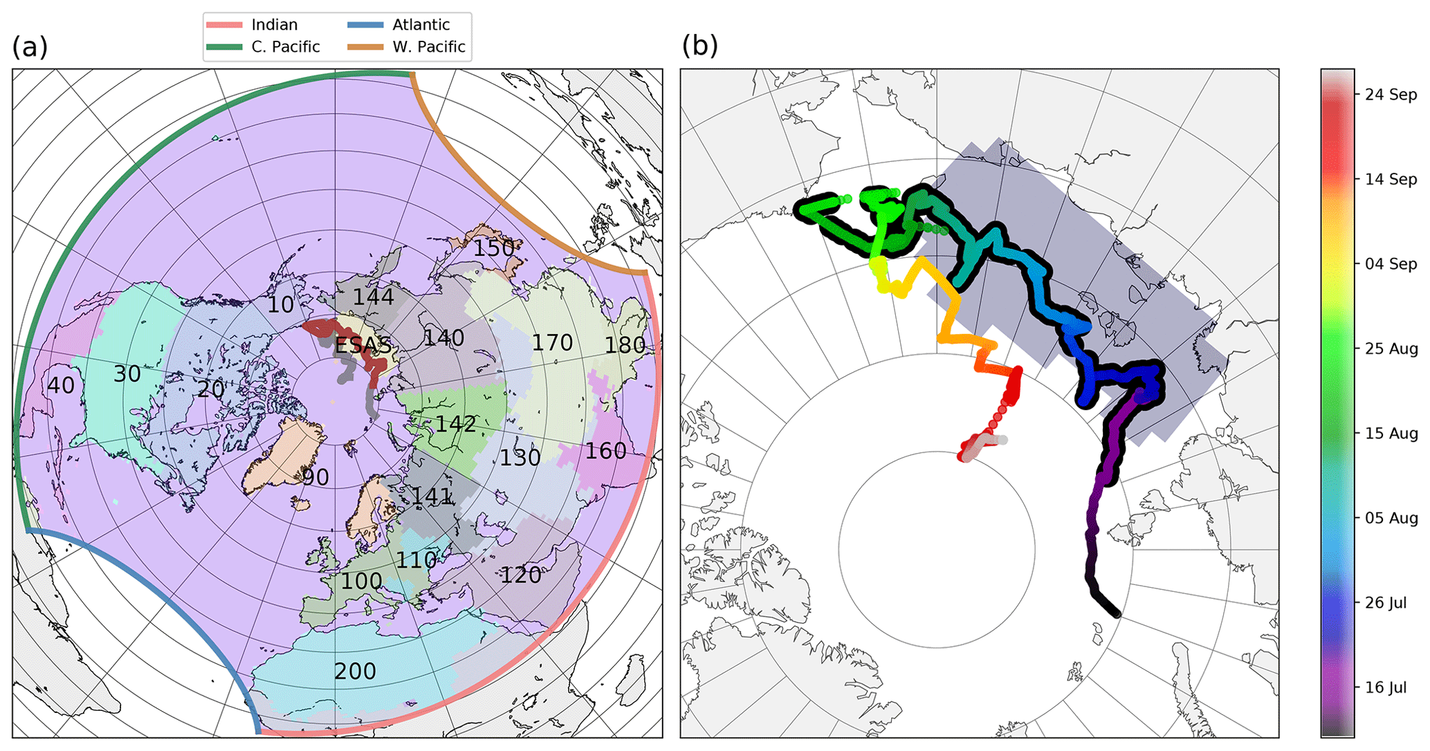
Figure 1 Path of the icebreaker Oden during the SWERUS-C3 campaign and domain of simulations. (a) The ship positions are represented by grey and brown lines, with brown parts corresponding to locations where isotopic observations where carried out. The area delimited by coloured lines is the domain of CHIMERE simulations used for this study (see Sect. 2.2). The shaded areas and associated numbers correspond to the regions and their IDs used to separate contributions from remote emissions to the observed signal, as detailed in Sect. 2.3. ESAS is the East Siberian Arctic Shelf. CHIMERE boundary conditions are split along the four sides of the domain as indicated by the coloured lines. (b) Zoomed-in view of the area covered by the campaign. The icebreaker's locations are coloured based on their corresponding dates. Ship positions with a black edge are locations where isotopic observations where carried out. More details on the campaign in Thornton et al. (2016a). The shaded area corresponds to the ESAS emission region used in our simulation set-up.

2.1 Campaign and instrument description

Observations were carried out during the SWERUS-C3 campaign aboard the Swedish icebreaker Oden between 14 July and 26 September 2014. The cruise path went through the central and outer Laptev and East Siberian seas and finally the Chukchi Sea to Point Barrow, Alaska, in a first leg (see Fig. 1). A second leg of the cruise headed north from Point Barrow back through the Chukchi Sea and into the Arctic Ocean. As shown in Fig. S1 in the Supplement, sea ice cover was present during a large portion of the campaign. Regions known to have active seafloor gas seeps (see Thornton et al., 2016a) occurred in both ice-free (in the Laptev Sea) and ice-covered (in the East Siberian Sea) regions.

Concentrations of total CH₄ were measured during the whole campaign using an off-axis cavity ring-down laser spectrometer from Los Gatos Research (LGR), Inc. (Model 0010, FGGA-24EP, Mountain View, California, USA). Air inlets were located at 9, 15, 20 and 35 m above the sea surface; air was pulled through all inlets continuously and analysed from one inlet at a time for 2 min before switching to the next inlet. Data were filtered using wind speed and direction to avoid contamination from the ship exhaust. As no local sources influenced our measurements, concentrations are similar at all levels. We concatenate measurements from all inlets indifferently for our study. The spectrometer was calibrated every 2 h using two synthetic air target gases; the target gases themselves were calibrated before, during and after the cruise to two NOAA Earth System Research Laboratory-certified standards for CH₄. The reported precision was 0.5 ppb. Further details on the campaign conditions and instrument configuration are available in Thornton et al. (2016a).

Isotopic ratios were measured only during the first leg of the campaign, from 14 July to 26 August (see Fig. 1), using an Aerodyne Research, Inc. (Billerica, MA, USA), direct absorption interband cascade laser spectrometer. This spectrometer measured the concentrations of the CH₄ isotopologues ¹²CH₄, ¹³CH₄ and CH₃D, the last of which is not discussed in the current paper. The more common isotope ratio mass spectrometry methods directly provide (as their name implies) an isotope ratio. In contrast, because the Aerodyne spectrometer measures the individual isotopologues, they must be individually calibrated before converting to ¹³C–CH₄ values; this method is described in McCalley et al. (2014).

2.2 Model description

The Eulerian model CHIMERE (Menut et al., 2013) was run to simulate total concentrations of CH₄ as well as partial ¹²CH₄ and ¹³CH₄ concentrations to compute CH₄ isotopic ratios afterwards using the following formula:

$$\begin{array}{}\text{(1)}& \mathit{\delta }{}^{\mathrm{13}}\mathrm{C}={\displaystyle \frac{{\left(\frac{\left[{}^{\mathrm{13}}\mathrm{C}\right]}{\left[{}^{\mathrm{12}}\mathrm{C}\right]}\right)}_{\text{sim}}}{{\left(\frac{\left[{}^{\mathrm{13}}\mathrm{C}\right]}{\left[{}^{\mathrm{12}}\mathrm{C}\right]}\right)}_{\text{ref}}}}-\mathrm{1},\end{array}$$

with ${\left(\frac{\left[{}^{\mathrm{13}}\mathrm{C}\right]}{\left[{}^{\mathrm{12}}\mathrm{C}\right]}\right)}_{\text{ref}}=\mathrm{0.0112372}$ being the reference ratio from Craig (1957).

The domain of simulations spans over most of the Northern Hemisphere, with a horizontal resolution of ∼100 km in order to include most contributions from distant sources (see Fig. 1). Similarly, the model uses 34 vertical levels from the surface up to 150 hPa to represent stratosphere-to-troposphere intrusions. A spin-up period of 6 months prior to the campaign was used to properly assess the impact of air masses transported for long periods before reaching the Arctic Ocean. The chemical sink of CH₄ by OH radicals is explicitly computed in CHIMERE using pre-computed fixed OH fields from the chemical model LMDz-INCA (Interaction with Chemistry and Aerosols; Hauglustaine et al., 2004; Folberth et al., 2006).

CHIMERE runs use the following input data streams: (i) meteorological fields downloaded from the European Centre for Medium Range Weather Forecasts (https://www.ecmwf.int) at 0.5^∘ resolution every 3 h, (ii) anthropogenic emissions aggregated at the CHIMERE resolution from the EDGARv4.3.2 database at 0.1^∘ horizontal resolution (Crippa et al., 2016), (iii) wetland emissions interpolated from the model ORCHIDEE at 0.5^∘ horizontal resolution (Ringeval et al., 2010), (iv) boundary CH₄ concentration fields extracted from the general circulation model LMDz (these global simulations include both the chemical sinks of OH and chlorine as well as their impact on the isotopic ratios, and Cl and OH fields are prescribed offline from the chemical model LMDz-INCA) and (v) and isotopic signatures of the different sources chosen from Sherwood et al. (2017).

The chemical sink by chlorine is not included in our set-up to keep simulations as light as possible. This sink can be separated into two main contributions: the upper stratosphere and the Arctic Ocean boundary layer. The upper stratosphere is not included in our model of simulation, but chlorine sink (and isotope fractionation) is explicitly accounted for in global LMDz simulations used as boundary conditions in our set-up. Regarding the Arctic Ocean boundary layer, the set-up by Thonat et al. (2017) was adapted to our case, including the boundary layer Cl sink using pre-computed fields from the model LMDz-INCA. It resulted in differences of concentrations lower than 1 ppb over the Arctic Ocean and less than 0.02 ‰ for the isotopic ratio of air masses, which is negligible compared to the signal we are inquiring into.

Other fluxes not included in our set-up play a significant role in the regional pan-Arctic budget, such as inland water bodies, wildfires and the sink in soil, but have limited impact on our observations. These fluxes were tested in our case and were quantified to cause differences in simulated concentrations lower than 2 ppb and less than 0.01 ‰ in simulated isotopic ratios at the locations sampled during the SWERUS-C3 campaign.

2.3 Atmospheric inversion of isotopic signature

Usually observations of δ¹³C–CH₄ are used to help with constraining methane fluxes and differentiating between different sources with known signatures. However, the intrinsic spatial and temporal variability in source isotopic signatures limits the robustness of this approach (e.g. Fisher et al., 2017, as illustrated in Sect. 3.1). Here, we conversely assume that total CH₄ is properly simulated by our model (as confirmed by the good performance of the model to reproduce total CH₄ concentrations, highlighted in Sect. 3.1) and that the relative contributions of various sources from various regions are correct. Thus we use δ¹³C–CH₄ observations to help reduce uncertainties in source isotopic signatures: we test the ability of the ship-based measurements to help constrain the isotopic signature of remote sources, such as wetland sources and oceanic emissions from the Laptev, East Siberian and Chukchi seas, dominant in the region explored during the campaign.

To do so, δ¹³C–CH₄ observations are implemented into a classical analytical Bayesian framework (Tarantola, 2005). The designed inversion system optimizes source signatures from different source types and different regions. At every time step when an isotopic observation is available, the system fits observations of isotopic ratios by altering the isotopic ratio in air masses coming from relevant source types and regions. Thus, the control vector contains one isotopic ratio value to optimize for each time step, each sector and each region, as detailed in Eq. (3) below.

The isotopic ratios of wetlands, solid fossil fuels, oil and gas, other anthropogenic sources from various land regions, and a potential variety of marine sources (gas field leaks, decomposing hydrates, degrading permafrost, etc.) from the East Siberian Arctic Shelf (ESAS) as well as from air masses coming from the sides and roof of our domain of simulations are optimized in the system. Apart from the ESAS, emissions are spatially differentiated into 23 geographical regions (see Fig. 1). Contributions from different regions and sectors are differentiated by computing so-called response functions by region, emission type and boundary side. That is to say, we carry out individual CHIMERE chemistry-transport simulations for every region, every type of emission and every side of the domain, with all the other emissions and boundary conditions being switched off, resulting in an ensemble of 98 response functions (23 regions × 4 sectors + ESAS + 4 sides + top).

The simulated isotopic final composition y(t) at every given time step t when an observation is available is retrieved by scaling relative contributions according to assumed source signatures (or original average composition for boundary conditions) as follows:

$$\begin{array}{}\text{(2)}& \mathit{y}\left(t\right)=\sum _{r\in \text{regions}}\sum _{s\in \text{sectors}}{\mathit{\alpha }}_{r,s}\left(t\right)\times {\mathit{\delta }}_{r,s}\left(t\right),\end{array}$$

with r and s varying over all available regions and sectors respectively; ${\mathit{\alpha }}_{r,s}^t$ ($\mathrm{0}<{\mathit{\alpha }}_{r,s}^t<\mathrm{1}$) is the relative contribution of the sector s from region r at time t, and ${\mathit{\delta }}_{r,s}^t$ is the signature (in ‰) of the sector s from region r at time t.

This linear relationship allows us to define the control vector x and the observation operator, linking the control vector to observations of isotopic ratios, to easily compute and scale the simulated isotopic composition:

$$\begin{array}{ll}{\displaystyle }& {\displaystyle }\mathit{y}\left(t\right)=\mathbf{H}\left(t\right)\mathit{x}\left(t\right),\\ \text{(3)}& {\displaystyle }& {\displaystyle }\text{ with }\left\{\begin{array}{l}\mathit{x}\left(t\right)={\mathit{\delta }}_{r,s}\left(t\right)\forall (r,s)\in \left(\text{regions}\right)\times \left(\text{sectors}\right),\\ \mathbf{H}\left(t\right)=\left({\mathit{\alpha }}_{r,s}\right(t){)}_{r\in \text{regions},s\in \text{sectors}}.\end{array}\right.\end{array}$$

Given the prior control vector x^b containing assumed source signatures before inversion, the observation vector y^o and the observation operator H, optimized signatures are obtained by solving the Bayesian problem equation:

$$\begin{array}{}\text{(4)}& {\displaystyle }{\mathit{x}}^{\mathrm{a}}{\displaystyle }={\mathit{x}}^{\mathrm{b}}+\mathbf{K}\left({\mathit{y}}^{\mathrm{o}}-\mathbf{H}{\mathit{x}}^{\mathrm{b}}\right),\end{array}$$

with $\mathbf{K}={\mathbf{P}}^{\mathrm{b}}{\mathbf{H}}^{\mathrm{T}}(\mathbf{R}+{\mathbf{HP}}^{\mathrm{b}}{\mathbf{H}}^{\mathrm{T}}{)}^{-\mathrm{1}}$ being the Kalman matrix.

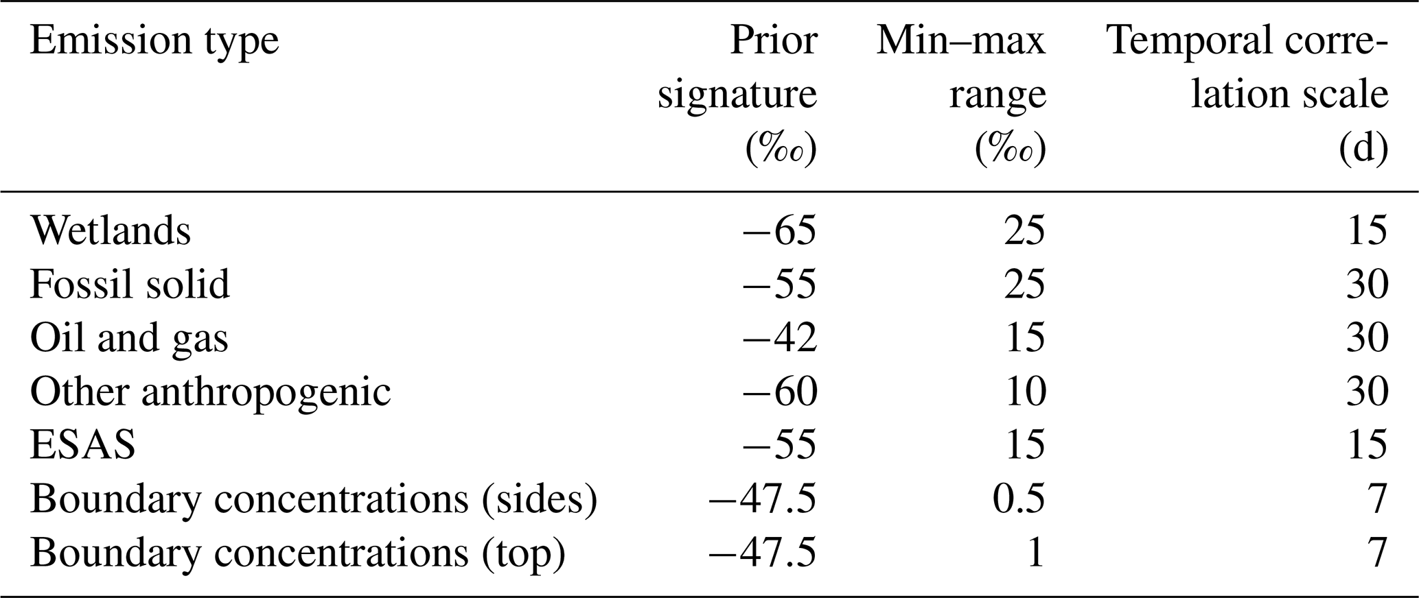
The matrix R represents uncertainties in the observations and in the capability of the model to reproduce them. In our case, we set them uniformly to 1.5 ‰ (1 ‰ from observation errors and 0.5 ‰ from simulation errors). The matrix P^b represents uncertainties and covariances in the prior knowledge we have on source signatures. We build the matrix P^b following the values in Table 1, deduced from Sherwood et al. (2017) and Sapart et al. (2017). Ranges and prior signatures for boundary conditions are deduced from global simulations with the model LMDz. Observation time steps are not optimized separately. Instead, we use temporal correlations in the P^b between different time steps. We represent temporal correlations between two time steps t_i and t_j as

$$\begin{array}{}\text{(5)}& r=\exp \left(-{\displaystyle \frac{|t_i-t_j|}{\mathit{\tau }}}\right),\end{array}$$

with τ being the temporal correlation scale of Table 1.

As shown in Table 1, the values of source signatures are not well known, and a very large range of signatures are available in the literature. To account for this large variety of realistic signatures, we carry out a Monte Carlo ensemble of 8000 inversions with varying prior signatures and uncertainties instead of running one single inversion. Prior signatures are sampled following a normal distribution with average and standard deviation from Table 1; the standard deviation is chosen as half of the min–max range. Uncertainties are sampled following a uniform distribution spanning over $[{\mathit{\sigma }}_{\text{ref}}/\mathrm{2},{\mathit{\sigma }}_{\text{ref}}]$, with σ_ref equaling half of the min–max range of Table 1.

In the end, we obtain hourly posterior signatures for each simulated sector and region for each of the 8000 inversions. Even though posterior signatures are available for each region and each sector at each observation time step, we do not inquire into the temporal variability in sources, as constraints provided by the SWERUS observations are very heterogeneous in time and space. Instead, we compute overall posterior distributions for each simulated sector and region based on an ensemble of 8 000 000 (8000 inversions × 1000 hourly observations). To minimize the impact of control vector components that are ill-constrained by the inversion, all data points are not evenly counted in posterior distributions. Posterior distributions of signatures are computed, accounting for all the Monte Carlo samples and weighted by the corresponding values of the sensitivity matrix KH (Cardinali et al., 2004), which gives an indicator of how much observations constrain one component of the control vector. The posterior optimal signature for each region and sector is computed as the maximum of the probability distribution.

Table 1 Isotopic signatures for the inputs in the CHIMERE model. The min–max range is deduced from existing literature (Sherwood et al., 2017; Sapart et al., 2017). The prior signature is computed as the centre of the min–max range.

3 Results and discussion

3.1 Forward modelling of total methane and isotopic ratio

Figure 2 shows observations of total CH₄ and of isotopic ratios as measured during the campaign and compared to simulations. The model CHIMERE reproduces most of the variability in the total CH₄ signal well. The average bias over the period is lower than 5 ppb, with a correlation of 0.66 between observations and simulations on an hourly basis. Most peaks spanning more than 1 d are properly represented in the model, proving the capability of the model to reproduce the synoptic variability in the observations. Smaller peaks are missed by the model, in particular on 5, 12 and 15 August, indicating that some local sources are not included in the model or are dispersed too quickly in the numerical realm. These could be local intense seeps that met along the ship's track or onshore wetlands not well represented with the model ORCHIDEE at 0.5^∘ horizontal resolution. We do not investigate further missing emissions, as most peaks are well explained by the model, which we assume is sufficient to carry out an inversion of isotopic signatures as described in Sect. 3.2.

When computing the intersect with the y axis of the linear fit between δ¹³C–CH₄ and total CH₄ (see Keeling plots in the Supplement), the observed isotope ratios point to an average generic Arctic source of −63.0 ‰, consistent with dominant biogenic sources in Arctic regions. The model reproduces this average signature well at −59.5 ‰. Observations highlight a strong synoptic variability in isotopic ratios in the Arctic, with a standard deviation of 0.50 ‰ and a range of 2 ‰. Most of this is missed by the model (see Fig. 2a, prior simulation). Simulated ratios with fixed (temporally and spatially) isotopic signatures for the emission sectors detailed in Sect. 2.3 barely exhibit any variations. The prior standard deviation is 0.22 ‰ (or 0.12 ‰ when removing the wetland event on 21 August), with a range of 1.5 ‰ (or 0.5 ‰). Considering the good fit of simulations to observations of total CH₄, the missing variability indicates that the classical assumption of uniform signatures for given sectors and regions is not valid in the Arctic, consistent with Ganesan et al. (2018) and Fisher et al. (2011). Contributions to modelled concentrations from different regions of a given emission sector can change much more than the variability in total CH₄, as indicated in Fig. 2. For instance, on 22 July, contributions from wetlands turn from a dominating Siberian influence to a North American one, causing a change of ∼30 ppb in the signal. Differences in the average wetland source signatures between these two regions of ∼20 ‰ (as suggested by Ganesan et al., 2018) would thus translate into ∼0.3 ‰ in measured isotopic ratio, partly explaining the corresponding observed event (see Fig. 2b).

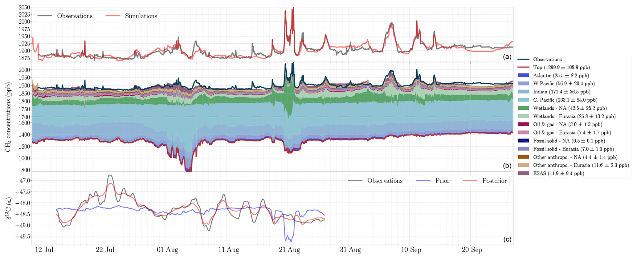
Figure 2 (a) Observed and simulated total CH₄ concentrations. (b) Simulated contributions to total CH₄ concentrations. Individual regions simulated by the model (see Fig. 1) are aggregated into two main continental components: North America (NA) and Eurasia. Light green areas depict Eurasian (mostly Siberian) wetlands, while dark green ones are North American wetlands. Shaded blue areas represent contributions from the sides of the CHIMERE simulation domain (see Fig. 1). Orange shades represent minor anthropogenic contribution. So-called “top” line gives the simulated concentrations originating from the lower stratosphere (i.e. from the top of CHIMERE simulation domain). Please note the gap in y axis scale at 1700 ppb, highlighted by the dashed line. (c) Observed and simulated isotopic ratios before (prior) and after (posterior) inversion.

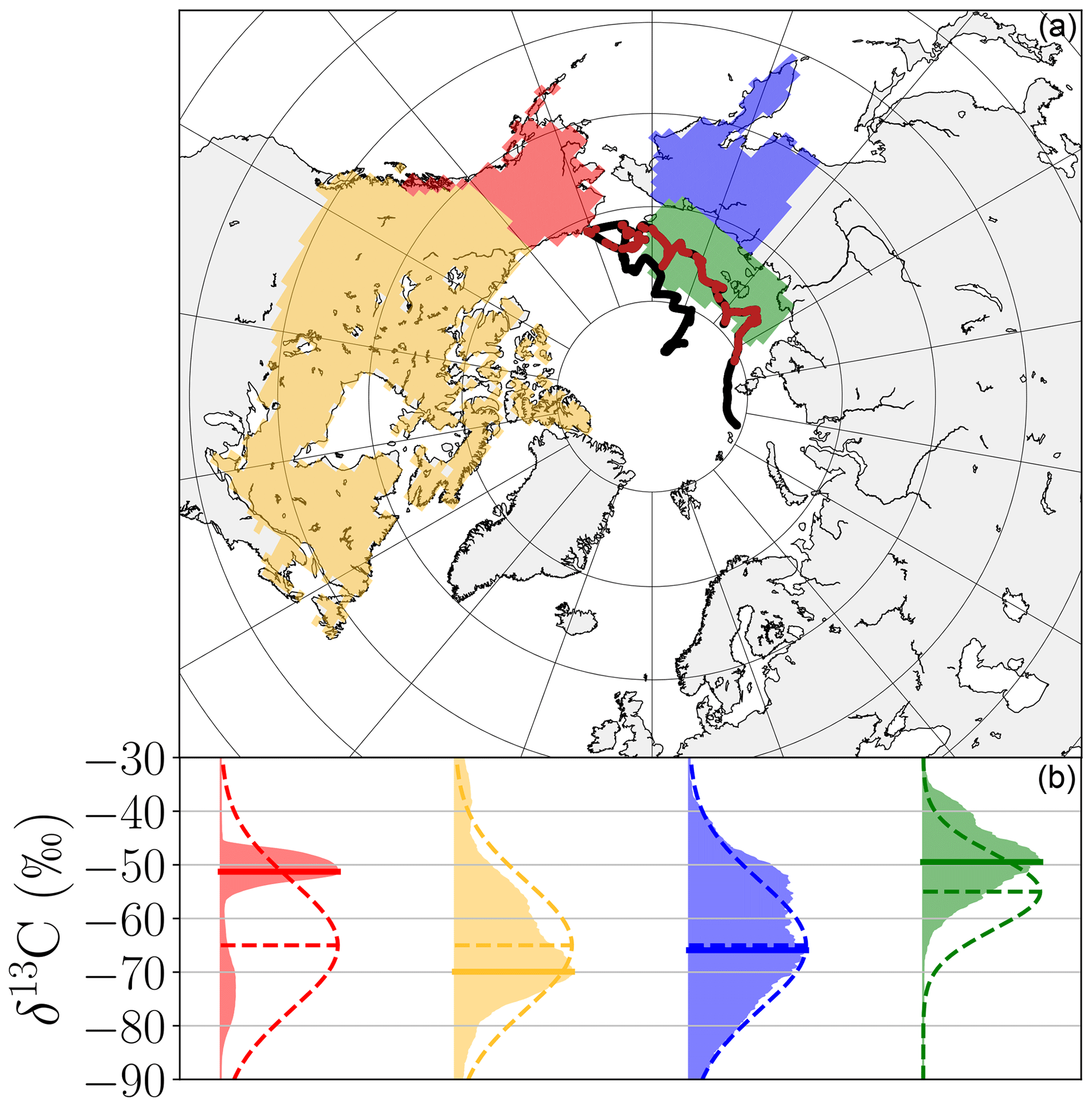
Figure 3 (a) Map of regions constrained by the observations in the inversion. For land regions, only wetlands are constrained. The green region corresponds to oceanic sources from the East Siberian Arctic Shelf. The ship path is indicated in black, with red points highlighting locations with available isotope observations. (b) Distribution of posterior hourly signatures as deduced by the inversion for regions constrained by the observations for the ensemble of 8000 Monte Carlo inversions (see details in Sect. 2.3). Prior signature distributions (dashed lines) are those of Table 1. The optimal posterior signatures, defined as the maximum of the posterior distribution, are highlighted by plain horizontal lines.

Still, more critical for the composition of air masses are the changes in very large-scale hemispheric contributions. As indicated by the blue shading in Fig. 2b, depending on the dominant large-scale transport patterns, contributions from the stratosphere and from the model lateral sides (located in the Tropics) can vary by more than 400 ppb within a few days. This corresponds to dominantly updraught or downdraught transport patterns, as illustrated by Fig. S2 in the Supplement. These very strong variations in total CH₄ enhance the impact of uncertainties in the vertical and horizontal distribution of isotopic ratios at the hemispheric scale. First, tropical air masses are influenced by tropical wetlands and anthropogenic emissions, causing a spatial and temporal variability in tropical isotopic ratio of up to 1 ‰, which is not accounted for in our CHIMERE set-up with fixed isotopic ratios at the simulation domain sides (see Sect. 2.2). Second, the vertical profiles of isotopic ratios in the Arctic (see simulated example from the global transport model LMDz in Fig. S3 in the Supplement) are very steep. Such gradients are poorly represented in most global models due to issues in the representation of the vertical transport or to the insufficiently quantified fractionating OH and chlorine sinks in the stratosphere and upper troposphere. These two sources of uncertainties in chemistry-transport models coupled with the strong real-world variations in stratospheric and tropospheric contributions could explain why the regional model CHIMERE does not reproduce the strong synoptic variability in δ¹³C–CH₄ observed during the SWERUS-C3 campaign. In particular, for the above-mentioned event on 22 July, contributions from the domain sides vary by more than 300 ppb. Such a variability in CH₄ contributions, associated with differences of a few percent per mille between the isotopic ratios of lower-stratosphere air masses and mid-latitude and low-latitude air masses, could explain the observed event.

Thus, the first-order variability in atmospheric isotopic ratios is due to a balance between non-regional transport-related hemispheric features and regional contributions of wetland, ocean and anthropogenic emissions.

3.2 Optimization of Arctic source signatures

Assuming that the mix of CH₄ sources is correct, we now attempt to separate hemispheric and regional contributions by optimizing source signatures for a set of geographical regions and different emission sectors in the Arctic as detailed in Sect. 2.3. Posterior isotopic ratios in Fig. 2c follow most of the variability in observations, indicating that the inverse method does fit the observations in a satisfying way. The rest of the signal is within the observation uncertainties of 0.1 ‰. This proves that even though the model is not perfect in representing the transport, it is reasonable to use simulated contributions to optimize isotopic signatures.

Figure 3 shows the posterior signature distributions as deduced from the 8000 Monte Carlo inversions for the four regions that are the most constrained by the observations, i.e. those weighted by the sensitivity matrix as detailed in Sect. 2.3. Accounting for the sensitivity matrix, it appears that only the roof boundary conditions (i.e. air masses from the lower stratosphere), ESAS emissions (i.e. emissions from the Laptev, East Siberian and Chukchi seas) and wetland regions on the shores of the Arctic Ocean are reasonably constrained by the SWERUS-C3 ship-based campaign. Even though anthropogenic emissions were optimized in our system, only the wetland emission sector is significantly constrained for land regions (Fig. 3). The lower-stratosphere signatures are in the short range of −48.5 to −46.5 ‰. Wetlands are suggested to have a heavier signature in Canada (optimal signature of −69.9 ‰) than in eastern Siberia (optimal signature of −65.9 ‰, with a node of similar importance at −55 ‰), consistent with Ganesan et al. (2018) and the compilation by Thornton et al. (2016b). Wetlands in Alaska exhibit a narrow posterior distribution at −51.3 ‰, with a secondary mode at −75 ‰. Alaska is thus well constrained by the inversion. However, the final value may suggest that the inversion has difficulties in differentiating collocated emissions and mixes the signal due to thermogenic sources with co-located wetland emissions, as is the case in Alaska with extensive extraction of raw oil and gas.

Posterior ESAS signatures are significantly shifted by more than 5 ‰ to −49.5 ‰ from the prior signature towards lighter values. This compares with previous studies and points towards a mix of different processes taking place in the Arctic Shelf, such as inputs from the seabed (James et al., 2016; Berchet et al., 2016; Skorokhod et al., 2016; Pankratova et al., 2018; Thornton et al., 2020). The posterior signature could thus be explained by mixed biogenic and thermogenic sources, confirming that ESAS emissions, possibly including a hydrate contribution, are not as depleted as wetland sources (Cramer et al., 1999; Lorenson, 1999).

Overall, the approach developed here reveals that the spatial and temporal variations in isotopic source signatures must be accounted for in order to properly represent δ¹³C–CH₄ observations. Such an approach does not allow us to reach definitive conclusions when considering the spread of the inferred regional isotopic signatures. However, it is crucial to account for isotopic ratios to avoid misallocating methane flux variations in methane inversions. We also show that atmospheric δ¹³C–CH₄ signals can be significant (larger than observation errors), indicating a good potential for the use of isotopic observations based on an oceanic campaign to improve our knowledge of the Arctic methane cycle. Finally, the weight of the boundary conditions in the signal points towards necessary progress in global simulations (including fractionating chemical reactions in the stratosphere) of CH₄ atmospheric isotopic ratios.

4 Conclusions

Observations of total atmospheric methane and isotopic ratio were carried out in summer 2014 in the Arctic Ocean during the SWERUS-C3 campaign aboard the Swedish icebreaker Oden. A unique continuous dataset of 45 d of atmospheric isotopic ratios over the Arctic Ocean is available from this campaign. Consistent with other campaigns in the region collecting flasks, the synoptic variability in atmospheric isotopic ratios in the Arctic is very strong, at ∼2 ‰, largely above observation error. Using forward simulations, we confirmed that the assumption of uniform isotopic signatures to represent emission sectors is invalid in the Arctic areas dominated by natural sources. We also exhibited the strong dependency of atmospheric isotopic ratios on large-scale changes in air mass origin (lateral boundaries of our simulation domain, corresponding to mid-latitude and low-latitude air masses; top boundaries corresponding to lower-stratosphere air masses). Based on a simplified inversion framework, the SWERUS-C3 data were used to infer isotopic source signatures of the Arctic regions and emission sectors. Due to the limited number of available observations and the important distance between sources and observations, our system was not able to provide any significant constraints on anthropogenic emissions and could optimize signatures from the ESAS and wetlands near the Arctic Ocean shores only. Wetland and oceanic ESAS source signatures were found to span a very wide range with a multimodal distribution for wetlands. The inversion also indicated that CH₄ emissions from the ESAS are composed of a mixture of dominant thermogenic methane, complemented by some biogenic methane.

Overall, only a strong spatial and temporal variability in emission signatures and in stratospheric isotopic ratios can explain the variability in observations. Therefore, our study points towards necessary improvements in simulating the first-order transport and chemistry of methane and its isotopes to reproduce large-scale hemispheric features, especially stratosphere to troposphere exchanges. This makes it necessary to improve (i) the quality of continuous isotopic measurements to capture the synoptic signal with even higher confidence, (ii) numerical chemistry-transport models so that the uncertainties in the first-order processes are at least 1 order of magnitude smaller than the regional signal, which is not the case in our study, and (iii) the mapping of isotopic emission signatures used as priors in inversions as initiated by Ganesan et al. (2018).