Description and Evaluation of the specified-dynamics experiment in the Chemistry-Climate Model Initiative

We provide an overview of the REF-C1SD specified-dynamics experiment that was conducted as part of phase 1 of the Chemistry-Climate Model Initiative (CCMI). The REF-C1SD experiment, which consisted of mainly nudged general circulation models (GCMs) constrained with (re)analysis fields, was designed to examine the influence of the large-scale circulation on past trends in atmospheric composition. The REF-C1SD simulations were produced across various model frameworks and are evaluated in terms of how well they represent different measures of the dynamical and transport circulations. In the troposphere there are large (∼40 %) differences in the climatological mean distributions, seasonal cycle amplitude, and trends of the meridional and vertical winds. In the stratosphere there are similarly large (∼50 %) differences in the magnitude, trends and seasonal cycle amplitude of the transformed Eulerian mean circulation and among various chemical and idealized tracers. At the same time, interannual variations in nearly all quantities are very well represented, compared to the underlying reanalyses. We show that the differences in magnitude, trends and seasonal cycle are not related to the use of different reanalysis products; rather, we show they are associated with how the simulations were implemented, by which we refer both to how the large-scale flow was prescribed and to biases in the underlying free-running models. In most cases these differences are shown to be as large or even larger than the differences exhibited by free-running simulations produced using the exact same models, which are also shown to be more dynamically consistent. Overall, our results suggest that care must be taken when using specified-dynamics simulations to examine the influence of large-scale dynamics on composition.

1 Introduction

Understanding the interaction between large-scale dynamics and atmospheric composition is important for understanding the past and future behavior of greenhouse gases (GHGs) and ozone-depleting substances (ODS). However, biases in large-scale atmospheric transport (both in terms of climatological means and interannual variability) remain large sources of uncertainty when assessing simulations of atmospheric composition. One approach to reduce this uncertainty has been to use numerical models that are constrained with meteorological fields taken from (re)analysis products. In this spirit, chemistry–climate models (CCMs) participating in the Chemistry-Climate Model Initiative (CCMI, Eyring et al., 2013) were asked to perform a so-called specified-dynamics simulation of the recent past (1980–2009) as part of the CCMI phase 1 hindcast experiment using large-scale flow fields taken from meteorological analyses and observed sea surface temperatures (SSTs) and sea ice concentrations (SICs). Modeling groups also performed parallel free-running integrations of the recent past using the same models and boundary conditions (i.e., SSTs and SICs).

While specified-dynamics simulations are commonly used in studies of atmospheric composition, it is not obvious that using analyzed meteorological fields necessarily improves simulation of the transport circulation (i.e., the tracer-independent properties of the flow) (Holzer and Hall, 2000) that is often summarized using measures like the stratospheric mean age (Hall and Plumb, 1994, among others). This is not only because of differences among reanalysis products, which can be large, especially in the stratosphere (e.g., Seviour et al., 2011; Abalos et al., 2015), but also because of the various ways in which a model may be constrained to analysis fields. Studies have long shown that transport computations using analyzed winds are very sensitive to how the large-scale flow is specified (e.g., Schoeberl et al., 2003; Meijer et al., 2004; Pawson et al., 2007). However, for historical reasons these sensitivities have been most rigorously explored in the context of offline chemical transport models (CTMs) and Lagrangian trajectory models, with several studies demonstrating the sensitivity of stratospheric transport to both the temporal sampling and averaging of the prescribed fields (e.g., Waugh et al., 1997; Bregman et al., 2006; Legras et al., 2005; Pawson et al., 2007; Monge-Sanz et al., 2007, 2012, 2013). By comparison, relatively less attention has been paid to assessing the credibility of large-scale transport in simulations using general circulation models constrained with reanalysis products either using so-called “nudging”, wherein the simulated meteorological fields are relaxed towards analysis fields (Kunz et al., 2012), or using approaches derived from data assimilation (e.g., Orbe et al., 2017b). While these studies have demonstrated large sensitivities in simulated transport to (at times arbitrary) choices in how the nudging is applied (e.g., Orbe et al., 2017b), it is difficult to draw general conclusions as it is not clear how specific these findings are to the particular model used and/or nudging approach implemented.

In addition to the lack of studies focused on evaluating simulated transport in nudged simulations, most intercomparisons focusing on atmospheric composition have primarily utilized CTMs – e.g., the Task Force on Hemispheric Transport of Air Pollution (TF HTAP; HTAP, UNECE LTRAP, 2007) and the Atmospheric Tracer Transport Model Intercomparison (TransCom; Patra et al., 2011) – or free-running simulations – e.g., the Atmospheric Chemistry and Climate Model Intercomparison Project (ACCMIP; Lamarque et al., 2013) and the SPARC Chemistry-Climate Model Validation Activity (CCMVal; Eyring et al., 2008). Thus, to the best of our knowledge, no intermodel comparison prior to CCMI has provided the output and experiments needed to rigorously evaluate the representation of dynamics and transport in primarily online nudged simulations. (Note that by “online” simulations we refer to those that have been produced using general circulation models.)

Another novelty of CCMI is that modeling centers provided both hindcast specified-dynamics and free-running simulations – herein referred to as REF-C1SD (simply SD for specified dynamics) and REF-C1 (simply FR for free-running), respectively – which presents a unique opportunity to compare the performance of specified-dynamics simulations relative to free-running integrations produced using the exact same versions of the models. Indeed, recent inquiries in this vein have proved illuminating, with Orbe et al. (2018) showing that the differences in interhemispheric transport (IHT) among the SD simulations are as large as the differences among FR integrations produced using the same models. More recently, Yang et al. (2019) analyzed the differences among tracers with more realistic anthropogenic emissions than those considered by Orbe et al. (2018), who focused only on tracers with zonally uniform sources, and also showed large differences in transport among the SD simulations. Unlike Orbe et al. (2018), who focused primarily on IHT differences in the context of parameterized convection in the tropics, Yang et al. (2019) focused on transport from Northern Hemisphere (NH) midlatitudes into the Arctic. Furthermore, they associated the spread in transport among the SD simulations to differences in the large-scale flow, specifically the poleward extent of the Hadley cell, evaluated in that study in terms of the near-surface meridional wind. This finding is particularly surprising, given that the meridional winds were specified in these simulations, albeit using a broad range of nudging techniques and sources of meteorological fields.

The findings presented in Orbe et al. (2018) and Yang et al. (2019) provide only a limited comparison of the large-scale flow fields among the REF-C1SD ensemble. More importantly, they provided no details about how the REF-C1SD simulations were actually implemented among the different models groups, information that is difficult – if not impossible – to access in the published literature. The goals of this study, therefore, are twofold: (1) document how the specified-dynamics hindcast simulations were implemented and (2) quantify key differences in first-order measures of the tropospheric and stratospheric dynamical and transport circulations. Via (2) our goal is to present a more comprehensive evaluation of the large-scale flow than presented in Orbe et al. (2018) and Yang et al. (2019) and to extend our analysis to the stratosphere, which has been evaluated in CCMI models primarily using the free-running REF-C1 experiment (Dietmüller et al., 2018). Note that, while Chrysanthou et al. (2019) presented the first comparison of the stratospheric residual circulation among the nudged CCMI hindcast runs, our analysis, which complements the findings presented in that study, has a broader scope by focusing on both the troposphere and the stratosphere and including discussions of large-scale transport.

It is important to note at the outset that there are several potential sources of differences among the SD simulations: (1) the use of different reanalysis fields, (2) differences in how the large-scale flow is constrained and (3) differences associated with biases in the underlying free-running models used to produce the SD simulations. When possible we try to isolate which source is most likely responsible for the spread among the simulations, but since (2) and (3) are in practice often related, and thus difficult to isolate from each other, we refer to them both using the general phrase “implementation differences”. We begin by discussing the models used and output analyzed in Sect. 2 and various aspects about how the simulations were implemented in Sect. 3, followed by a comparison of key large-scale dynamical and transport properties in Sects. 4 and 5. Brief conclusions in Sect. 6 are followed by details specific to each individual model (Appendix).

2 Methodology

2.1 Models and experiments

The CCMI hindcast experiment consisted of both free-running REF-C1 (FR) and specified-dynamics REF-C1SD (SD) simulations, both of which were constrained with observed SSTs and SICs. Here we report the details of how the SD simulations were implemented among models, based on feedback we received in response to a survey that was distributed among CCMI model contact leads. Among those simulations we only show results from output that was uploaded to the British Atmospheric Data Centre (BADC) archive (ftp://ftp.ceda.ac.uk, last access: 10 January 2019) and/or provided to us via personal communication (2018). Output from the WACCM and CAM simulations was obtained from the NCAR Earth System Grid portal (https://www.earthsystemgrid.org/, last access: 6 January 2019). Table 1 lists the modeling groups that responded to our survey, what type of model was used for the SD simulation (offline CTM or online nudged CCM) and which source of meteorological fields was used. We also note whether a parallel free-running simulation was performed, since the subset of models for which both FR and SD simulations were performed comprises a unique ensemble within the hindcast experiment (hereafter referred to with an asterisk as SD^*) that is ideal for evaluating the performance of specified-dynamics simulations relative to free-running simulations.

Table 1 List of the REF-C1SD model simulations that were conducted in support of CCMI phase 1. Columns 2 and 3 indicate whether REF-C1SD was produced using an offline CTM or online nudging, as well as the source of the constraining analysis fields, respectively. Columns 4 and 5 list the fields that were constrained in the REF-C1SD simulations, with D and ζ denoting the divergence and vorticity fields, respectively, as well as the timescales over which nudging was performed. For the WACCM and CAM simulations, additional nudging was performed with respect to TAUX and TAUY, SHFLX, and LHFLX (surface stress, latent heat flux and sensible heat flux). Note that column 5 only broadly summarizes the nudging timescales applied in the REF-C1SD simulations for sake of brevity. We refer the reader to the Appendix for more information about cases where τ exhibited a functional dependence (on pressure, for example).

The superscript ^a in column 1 indicates that a corresponding free-running REF-C1 simulation was also performed using the same underlying model code. ^b Note that the GEOS replay and WACCM C1SD simulations are constrained with MERRA analysis fields. For more on the difference between the analysis and assimilated fields we refer the reader to Orbe et al. (2017b). ^c The output for these simulations was not available for analysis. n/a – not applicable.

We note that typically only one SD experiment was submitted per modeling group. However, as in Orbe et al. (2017a, 2018) and Yang et al. (2019) we include two SD simulations from NASA and NCAR, denoted in all figures using a color convention that is similar to what was used in those studies. In particular, the two NASA SD simulations here refer to an offline integration of the NASA Global Modeling Initiative (GMI) chemical transport model (Strahan et al., 2007, 2016) as well as an online simulation of the Global Earth Observing System (GEOS) general circulation model, both constrained with MERRA meteorological fields (Reinecker et al., 2011) (not MERRA-2, Gelaro et al., 2017). We also present two SD NCAR simulations in which WACCM was nudged to MERRA on two different relaxation timescales. Further details of those (and all other) simulations are presented in the Appendix. Finally, in addition to differences among the REF-C1 and REF-C1SD experiments, the models differ widely in terms of their horizontal resolution, vertical resolution and choices of subgrid scale (i.e., turbulence and convective) parameterizations. For a more comprehensive review of these details we refer the reader to Morgenstern et al. (2017). In all cases only a single simulation was taken from the REF-C1 experiments for models that submitted multiple ensemble members. This was usually the r1i1p1 simulation; the only exception to this was the CNRM-CM 5-3 simulation, for which only the r1i1p2 output was available on the BADC archive.

2.2 Diagnostic output

While the primary purpose of this study is to document how the REF-C1SD experiment was implemented among models (Sect. 3), we also take the opportunity to provide more extensive comparisons of the large-scale flow and transport fields than what was shown by Orbe et al. (2018) and Yang et al. (2019) (Table 2). In order to compare the flow among the models we focus on basic first-order measures, including the three-dimensional winds (U, V and ω) and temperatures (T) in the troposphere. (Note that the vertical velocity (w) was available in all simulations and then converted into pressure velocity through the relation $\mathit{\omega }=-w\mathit{\rho }g$, where ρ and g are density and gravity, respectively.) In the stratosphere, the dynamical circulation is more naturally quantified using the transformed Eulerian mean (TEM) residual meridional (v^*) and vertical (w^*) velocities (Andrews et al., 1987). Following Dietmüller et al. (2018) we note that since w^* was calculated slightly differently among models, specifically with respect to the conversion of the Lagrangian tendency of air pressure, we also derived w^* independently from v^* by continuity, as in that study. Comparisons of w^* between the model output and the values inferred from v^* are presented in Sect. 4 and result in no major differences with respect to our main findings.

Table 2 List of the model simulations for which the dynamical fields (U, V, T, ω, v^* and w^*) and both chemical and idealized tracers (O₃, N₂O, Γ_NH and Γ_STRAT) were available as (monthly mean) output. Checkmarks (crosses) denote fields that were (were not) output in simulations. Note the same output was also available for all corresponding free-running runs in those cases in which both REF-C1 and REF-C1SD simulations were provided (see column 1, Table 1). Open circles denote tracers that were integrated in simulations but not implemented correctly.

^* Output for WACCM-5hr was available only for years 2000–2009 for several variables.

In addition to circulation diagnostics we also include comparisons of ozone (O₃), nitrous oxide (N₂O) and the stratospheric mean age (Γ_STRAT) – the mean transit or “elapsed” time since air last contacted the tropical tropopause (i.e., Hall and Plumb, 1994; Waugh and Hall, 2002). We also present comparisons in the stratosphere of the NH midlatitude mean age (Γ_NH), defined as the mean transit time since air last contacted the NH midlatitude surface (Waugh et al., 2013; Orbe et al., 2018), since few models integrated both the stratospheric and NH midlatitude mean age tracers (Table 2). Thus, while they physically capture similar aspects of the transport circulation, the output from the different age tracers comprises different groups of models within the larger SD ensemble and therefore provides relatively independent perspectives on the transport differences among the simulations. We make the ages more comparable by subtracting off a reference mean age value, evaluated here as the mean age at 100 hPa, averaged over 10^∘ S to 10^∘ N. This also corrects for the fact that the stratospheric mean age tracer was implemented differently among different models, with some models applying the lower boundary condition globally at the surface (vs. only in the tropics). A similar approach was used by Dietmüller et al. (2018), except their reference was defined relative to the tropical tropopause in each model.

For our analysis of tropospheric variables we interpolated all output from native model levels to a standard pressure vector with four pressure levels in the stratosphere (10, 30, 50 and 80 hPa) and 19 pressure levels in the troposphere spaced every 50 hPa between 100 and 1000 hPa (Orbe et al., 2018). Unlike in the troposphere, the stratospheric circulation and tracer output was requested on 31 constant pressure surfaces from 1000 to 0.1 hPa so no additional interpolation in the vertical was required. However, for some models (i.e., MOCAGE, CAM, WACCM, MRI) the output was available on different pressure levels that had to be interpolated manually to the 31 pressure levels. For both tropospheric and stratospheric variables we also interpolated in the horizontal to the same 1^∘ latitude by 1^∘ longitude grid as in Orbe et al. (2018). Only monthly mean output is used as that is all that was available for the quantities analyzed here.

Finally, when possible we compare the output from SD simulations with fields from ERA-Interim (hereafter ERA-I) (Dee et al., 2011), MERRA (Reinecker et al., 2011) and JRA-55 (Kobayashi et al., 2015). For the case of the TEM circulation components, v^* and w^*, we have used the common grid (2.5^∘ latitude by 2.5^∘ longitude) output from the SPARC Reanalysis Intercomparison Project (S-RIP) dataset (Martineau et al., 2018). Note that only ω^* was available from the S-RIP fields (units: Pa s⁻¹), whereas the CCMI output is in terms of w^* (units: m s⁻¹), thus requiring that we convert the S-RIP fields to w^* using the following relation: ${\stackrel{\mathrm{‾}}{w}}^{*}=-\frac{H}{p}{\stackrel{\mathrm{‾}}{\mathit{\omega }}}^{*}$, where $H={\text{RT}}_s/g$ is a mean scale height of the atmosphere, here taken to be 7 km, corresponding to T_s∼240 K, a constant reference air temperature (see Eq. A16 in Gerber and Manzini, 2016).

2.3 Metrics

For all variables we first compare 10-year 2000–2009 climatological mean meridional profiles among the SD simulations and among the reanalysis fields (when available) to which they were initially constrained (Sect. 4.1). Then we compare the temporal variability of the simulations, first comparing the seasonal cycle amplitude (SCA) and phase among the simulations, also for the 2000–2009 period, both with respect to the other simulations and with respect to the reanalysis products (Sect. 4.2). As in Barnes et al. (2016) we define the SCA as the climatological seasonal cycle of the zonally averaged fields at every pressure level and latitude (note we do not apply their 31 d filter as they were using daily data and we are using monthly data). The SCA is then defined as the difference between the maximum and minimum of the seasonal cycle, respectively designated throughout as τ_max and τ_min. In addition, throughout we normalize the SCA by its climatological annual mean value in order to account for the fact that for some variables the seasonal cycle is small so that discrepancies in (unnormalized) SCA values may appear larger than they actually are, relative to the climatology. Care is taken throughout to identify those cases when the seasonal cycle amplitude is small.

In addition to the seasonal cycle we also assess how well the simulations covary with each other on interannual timescales over years 1980–2009. As such, our assessment of interannual variability, which evaluates only the degree of correlation between time series, differs from previous studies (Chrysanthou et al., 2019), in which time series were further decomposed in terms of different modes of interannual variability (i.e., the El Niño–Southern Oscillation, the Quasi-Biennial Oscillation, etc.). More precisely, for each member within the SD ensemble we identify a given variable χ for which we first remove the linear trend and then calculate the correlation coefficient between the annual mean time series corresponding to that ensemble member i and the annual mean time series of its corresponding ensemble mean. For example, corr(i)_U,ERA corresponds to the correlation coefficient between the detrended annually averaged zonal winds of simulation i and the (also detrended and annually averaged) zonal winds averaged over the ensemble of simulations constrained with ERA-Interim fields. We also evaluate how well each simulation varies relative to the entire SD ensemble, the mean of which will average out differences among the reanalysis products, denoted hereafter as corr(i)_χ,SD. Correspondingly, for any given ensemble of SD simulations M (e.g., ERA-I, MERRA, JRA-55, SD) consisting of N members, the ensemble mean of corr(i)_χ,M is throughout denoted as ${\stackrel{\mathrm{‾}}{\text{corr}}}_{\mathit{\chi },M}\equiv \frac{\mathrm{1}}{N}{\sum }_{i=\mathrm{1}}^N\text{corr}(i{)}_{\mathit{\chi },M}$.

Finally, we conclude our analysis by comparing trends of the various measures, evaluated here simply as the linear fit to the deseasonalized time series. While previous studies have already cautioned about the suitability of inferring trends from either reanalyses (Abalos et al., 2015) or nudged experiments (Chrysanthou et al., 2019), those studies focused on the lower stratosphere (specifically, the transformed Eulerian mean circulation), and it is not clear to what extent their conclusions about trends apply to other dynamical and constituent fields.

3 Implementation of the REF-C1SD simulation

Here we summarize key aspects describing how the SD simulations were implemented. For more detailed descriptions of implementation in the individual models we refer the reader to the Appendix. As such, both sections complement the information provided in Table S30 in the Supplement of Morgenstern et al. (2017).

3.1 Nudging vs. CTM

Most of the REF-C1SD simulations were performed as nudged simulations using online CCMs (MRI-ESM1r1, GEOS, HadGEM3-ES, GFDL-AM3, EMAC, CNRM-CM 5-3, CHASER (MIROC-ESM), CESM WACCM, CESM1 CAM4-chem, CCSRNIES MIROC3.2, IPSL, UMUKCA, CMAM), although a few groups also submitted results from offline CTMs (TOMCAT CTM, MOCAGE CTM and NASA GMI-CTM). Note that the GEOS REF-C1SD simulation did not use a standard nudging approach but, rather, the “replay” approach, which involves reading in MERRA fields and recomputing the analysis increments, which are applied as a forcing to the meteorology at every model time step (Orbe et al., 2017b; see Appendix for more information). In addition, note also that output from the HadGEM3-ES, and GFDL-AM3 simulations was not available so our analysis comprises a total of 13 simulations produced using online models and 3 simulations produced using CTMs.

3.2 Sources of meteorological fields

Large-scale meteorological fields from the three reanalysis products ERA-I, MERRA and JRA-55 were used to constrain the REF-C1SD simulations. Although NCEP/NCAR (Kistler et al., 2001) fields were also used in the GFDL simulations those fields are not analyzed here since that output was not available. Among the ERA-I-constrained simulations, all use 6-hourly instantaneous fields, although differences may still arise among those simulations due to differences in how the analysis fields were interpolated to the models' native grids. By comparison, among the MERRA-constrained simulations, there are additional differences related to the fact that multiple MERRA products were used. In particular, while the GMI CTM simulation used the 3-hourly time-averaged assimilated fields, the GEOS and WACCM REF-C1SD simulations were constrained using 6-hourly instantaneous analysis fields. An examination of the differences in stratospheric transport implied by using assimilated vs. analysis fields for the GEOS model was presented in Orbe et al. (2017b). Specifically, within the context of replay they showed that the use of analysis fields produced stratospheric mean age values that were consistently younger than if assimilated fields were used, irrespective of their temporal sampling (3-hourly vs. 6-hourly).

3.3 Boundary conditions

Most of the REF-C1SD simulations use the Hadley Centre Ice and Sea Surface Temperature (HadISST) dataset (Rayner et al., 2003), as recommended. Some simulations, however, were forced with climatological SSTs and SICs taken from other datasets derived both from models (TOMCAT CTM) and other observational sets. The latter include simulations constrained with monthly mean SSTs as used in the AMIP simulations and described in Hurrell et al. (2008) (IPSL LMDz-REPROBUS). The former include simulations that were constrained with SSTs from Reynolds et al. (2000) (the NASA GMI-CTM simulation) and ERA-Interim (EMAC).

3.4 Constrained variables, nudging spatial domains and relaxation timescales

Two major sources of differences among the nudged simulations are the choice of large-scale fields and nudging timescales with which the model fields were constrained to the analyses. For example, while nearly all the REF-C1SD simulations are constrained to the east–west and north–south components of the horizontal wind (U, V), some models (EMAC, TOMCAT) were nudged to the divergence and vorticity fields. In addition, several simulations also nudged to temperature (T) (or potential temperature, as in UMUKCA), water vapor, (the logarithm of) surface pressure, surface stress, and latent and sensible heat fluxes. A few models also applied nudging in spectral space (EMAC).

Nudging timescales and nudging domains varied widely among the different simulations, where we define the nudging relaxation time constant τ such that the nudging increment for variable χ is proportional to (${\mathit{\chi }}_{\text{analysis}}-{\mathit{\chi }}_{\text{model}})/\mathit{\tau }$ (note that τ has units of hours). In particular, τ ranged from as low as 5 h in some simulations (CNRM-CM 5-3, WACCM-5hr) to as long as 60 h in others (GFDL-AM3), with some simulations applying spatially uniform nudging (e.g., CMAM and UMUKCA), while in others τ depends explicitly on pressure or model level (GFDL-AM3, MRI-ESM1r1, EMAC).

3.5 Sources of convective mass fluxes

In addition to differences in the resolved flow among the simulations, another large source of differences is the (parameterized) convective mass fluxes used to simulate convective transport. These were either taken from the same analysis dataset from which the large-scale flow fields were obtained (the NASA GMI-CTM) or recalculated online using the model's own convective parameterization. The latter approach was used mainly in the nudged simulations, although some offline models also recomputed the convective mass fluxes.

A broad range of convective parameterizations are used including relaxed and/or triggered schemes as described in Moorthi and Suarez (1992) and Zhang and McFarlane (1995) (CESM1 CAM4-chem and WACCM, CMAM, GMI-CTM), nearly instantaneous adjustment schemes along the lines of Arakawa and Schubert (1974) (CCSRNIES MIROC3.2, CHASER MIROC-ESM, MRI-ESM1r1), and diagnostic closure schemes based on large-scale moisture or mass convergence similar to Tiedtke (1989) (TOMCAT CTM, EMAC).

4 Comparisons of large-scale flow among REF-C1SD simulations

We now present a comparison of various large-scale flow measures of the REF-C1SD simulations, both in terms of their climatological mean distributions as well as their seasonal and interannual variability. Throughout, special focus will be placed on interpreting the sources of differences among the REF-C1SD simulations, specifically with respect to the use of different reanalysis fields vs. differences related both to how the large-scale flow fields are constrained and to underlying free-running model biases. To this end, Table 3 summarizes these three potential sources of spread among the SD ensemble and highlights key examples of each source as demonstrated by the simulations analyzed in this study.

Table 3 Below we identify three distinct sources of differences among the SD simulations. We distinguish between differences associated with the use of different reanalysis products (row 1) vs. differences associated with how the large-scale flow fields are specified (row 2) as well as underlying free-running model biases (row 3). All sources are present in the REF-C1SD ensemble considered in this study.

4.1 Climatological distributions

We begin by comparing meridional profiles of the 2000–2009 climatological mean zonally averaged zonal winds at 850 and 300 hPa, respectively chosen in order to evaluate the representation of the near-surface eddy-driven component of the zonal winds over midlatitudes and the subtropical jet (e.g., Barnes and Polvani, 2013). As shown in Fig. 1 U₈₅₀ and U₃₀₀ compare very well among the SD simulations (Fig. 1a). Comparisons of the temperature field also reveal only small (∼1–2 K) differences among the SD simulations (Fig. 1b), with the exception of one outlier (i.e., IPSL SD). Further inspection of that simulation confirms that it was nudged to ERA-I U, V and T using a height-dependent nudging timescale, with weaker nudging at lower pressures. This may explain why the biases in that outlier are larger in the upper troposphere, with values of T₃₀₀ in that simulation corresponding well with values from the free-running simulation produced using that same model (Fig. S1, Table S3 in the Supplement, rows 2 and 3). That outlier aside, overall we conclude that the climatological zonal mean distributions of both the zonal winds and temperature fields are well constrained in the troposphere in the SD simulations, relative both to the reanalysis products and to the others members within the SD ensemble.

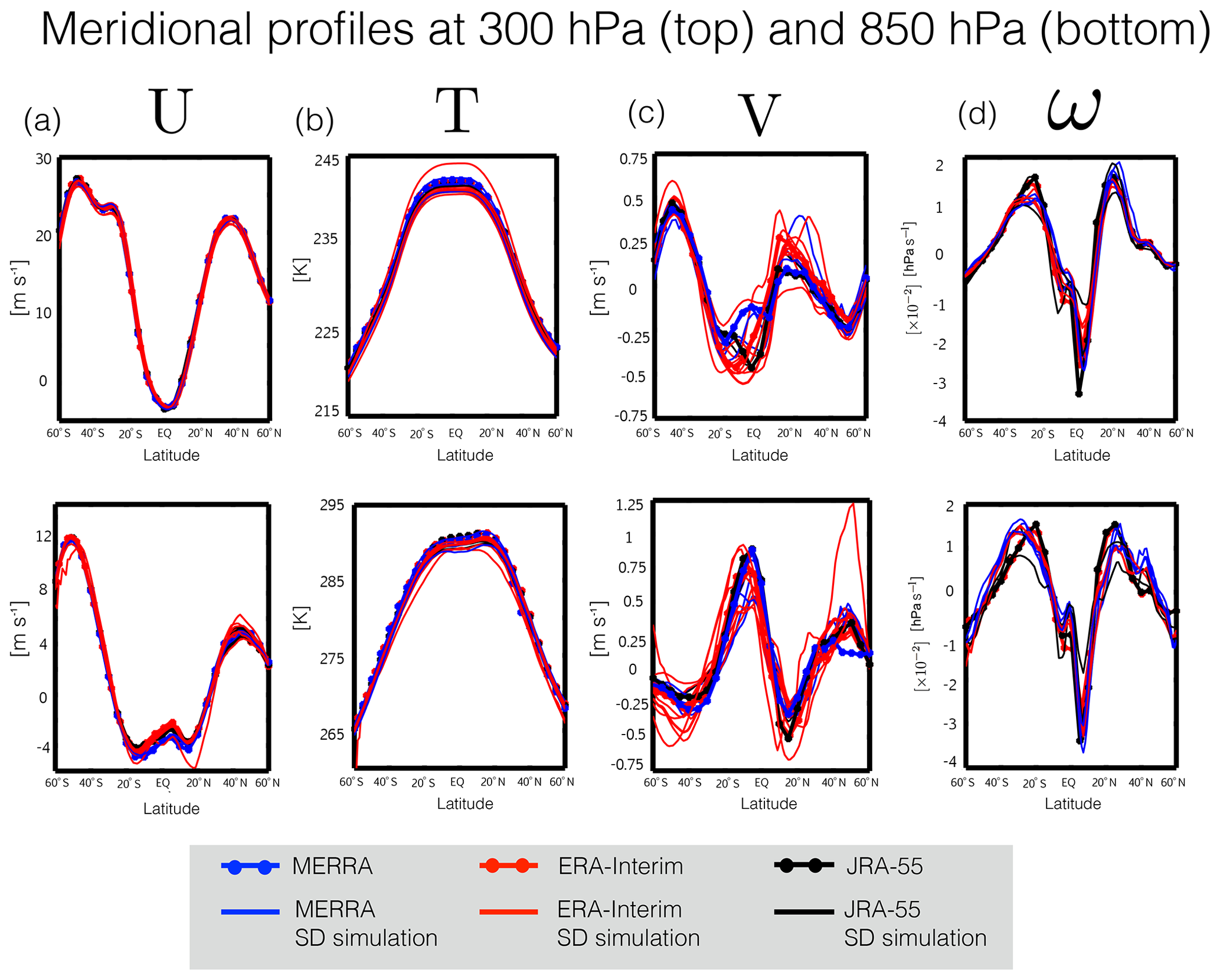
Figure 1 Meridional profiles of the 2000–2009 climatological annual mean (a) zonal mean zonal wind (U), (b) zonal mean temperature (T), (c) zonal mean meridional wind, and (d) zonal mean pressure velocity (ω) at 300 hPa (top panels) and 850 hPa (bottom panels). Red/blue/black lines correspond to SD simulations constrained with ERA-Interim/MERRA/JRA-55 reanalysis fields. Red/blue/black dotted lines correspond to the raw ERA-Interim/MERRA/JRA-55 meteorological fields. Note that MERRA assimilated fields are shown, for which ω is not available.

By comparison to the zonal winds and temperatures, the meridional winds (Fig. 1c) reveal substantially larger differences among the SD simulations, with differences in V₈₅₀ approaching 0.4 m s⁻¹ in the tropics and Southern Hemisphere (SH) midlatitudes and almost 1 m s⁻¹ over NH midlatitudes (Fig. 1c, bottom) (Yang et al., 2019). In the upper troposphere the differences in V₃₀₀ are equally as large, peaking at 0.4 m s⁻¹ (or nearly 80 % of the ensemble mean climatology) in the tropics and 0.3 m s⁻¹ (also 80 % of the climatological ensemble mean value) over the NH subtropical jet. Furthermore, although there are large differences among the reanalysis products, especially between MERRA vs. ERA-I and JRA-55 in the tropics (Table 3, row 1), the differences among the SD simulations cannot be entirely understood in terms of the different reanalyses. Rather, a large fraction of the SD ensemble spread in V is spanned solely by simulations constrained with ERA-I fields (note that the differences among the MERRA and JRA-55 simulations are also large but appear smaller partly because those subsets of SD simulations contain fewer members).

In addition to the meridional winds we also find large differences in ω₈₅₀ approaching 0.02 hPa s⁻¹ in the tropics and 0.01 hPa s⁻¹ in the subtropics, or ∼60 % and ∼50 % relative to the ensemble mean climatologies, respectively (Fig. 1d, bottom). The differences aloft captured by ω₃₀₀ are similar in magnitude (Fig. 1d, top). As with the meridional winds the largest differences occur in the (sub)tropics and are not obviously related to differences associated with the use of different reanalysis products, although we note that ω was not part of the MERRA assimilated (ASM) collection analyzed here, which limits our interpretation somewhat. Furthermore, in all simulations ω was computed online and was not constrained directly to the reanalysis fields. Therefore, unlike the fields U, V and T, the differences in ω among the SD simulations not only reflect differences associated with the source of analysis fields but also the way in which ω was calculated online in models.

Comparisons of meridional profiles of the TEM circulation and the chemical and passive tracer distributions in the stratosphere (Fig. 2) reveal that, overall, the differences in the TEM circulation among the SD simulations are even larger than the meridional and vertical wind differences in the troposphere. Specifically, values of $v_{\mathrm{30}\mathrm{hPa}}^{*}$ range between −0.1 and 0.1 m s⁻¹ in the subtropics (Fig. 2a, top), while differences in $v_{\mathrm{80}\mathrm{hPa}}^{*}$ approach 0.4 m s⁻¹ over northern and southern midlatitudes (or ∼100 % the climatological mean ensemble mean value) (Fig. 2a, bottom). Similarly, the differences in $w_{\mathrm{80}\mathrm{hPa}}^{*}$ (Fig. 2b) approach ∼0.0008 m s⁻¹ (also ∼100 % the ensemble mean climatological value). Chrysanthou et al. (2019) noted similarly large differences in w^* among the REF-C1SD simulations, although they examined a slightly different region in the stratosphere (10 and 70 hPa vs. the 30 and 80 hPa pressure levels examined here).

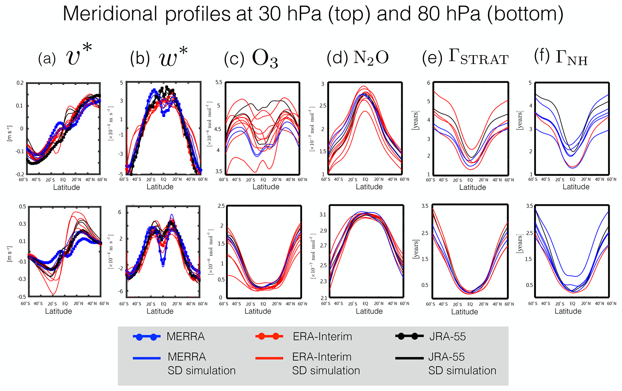
Figure 2 Meridional profiles of the 2000–2009 climatological annual mean (a) residual meridional velocity (v^*), (b) residual vertical velocity (w^*), (c) ozone (O₃), (d) nitrous oxide (N₂O), (e) stratospheric mean age (Γ_STRAT) and (f) Northern Hemisphere midlatitude mean age (Γ_NH). Profiles are shown for 30 hPa (top) and 80 hPa (bottom). Red/blue/black lines correspond to SD simulations constrained with ERA-Interim/MERRA/JRA-55 reanalysis fields. For the cases of v^* and w^* red/blue/black dotted lines correspond to the S-RIP TEM velocities derived from ERA-Interim/MERRA/JRA-55 meteorological fields.

As described earlier, the differences in the w^* fields may be exaggerated by the fact they also potentially reflects inconsistencies in how that calculation was performed among modeling groups. Therefore, we also derive w^* from continuity as outlined Dietmüller et al. (2018), and, consistent with their results, we find that the independent derivation of w^* using v^* does produce noticeable, and even larger, differences in the values of w^* (Fig. S2 in the Supplement). (Note that, in order to facilitate comparisons with Dietmüller et al., 2018 (specifically their supplementary Fig. S2), we also show averages over 20^∘ S and 20^∘ N.) However, although we find that the absolute values of w^* differ between the output provided on the BADC archive vs. our offline calculations inferred from v^*, we nonetheless find that the differences in w^* are of similar magnitude across the SD ensemble, irrespective of which calculation is used. Therefore, despite potential inconsistencies in how w^* was calculated among modeling centers, the fact that it differs widely among SD simulations is a robust result.

Although for some variables and locations (e.g., w^* at 30 hPa, Fig. 2b, top) the TEM circulation values are clustered by the reanalysis product, thus indicating that differences in the simulations appear to be primarily driven by differences among the reanalyses, this does not generally hold across variables and different locations in the stratosphere. This is particularly true for the chemical and idealized tracers, including O₃ at 80 hPa (Fig. 2c, bottom), with values spanning nearly 100 ppb (or 30 % the climatological mean value), and for N₂O at 30 hPa (Fig. 2d, top), for which differences over southern midlatitudes approach ∼ 100 % the climatological mean value (Table 3, row 3). For both tracers the ensemble spread is spanned nearly entirely by the ERA-I ensemble, although, as discussed earlier, this may simply reflect the overrepresentation of that reanalysis product in the SD ensemble. Large differences among the simulations constrained with the same reanalysis fields are also evident in Γ_STRAT (Fig. 2e) and Γ_NH (Fig. 2f), for which the SD ensemble spread is dominated by differences among the ERA-I and MERRA ensembles, respectively (Table 3, row 2). Note that this partly reflects the fact that more Γ_STRAT output was available from ERA-I simulations (and more Γ_NH output from MERRA simulations). Furthermore, among the MERRA-constrained simulations of Γ_NH three of the simulations represented utilize similar models (e.g., WACCM-5hr, WACCM-50hr and CAM). Therefore, the particular details of the mean age differences discussed are likely sensitive to the choice of ensemble members and ensemble size.

4.2 Temporal variability

4.2.1 Seasonal cycle

The previous section showed that there are large differences in the climatological mean properties of various dynamical and transport fields among the SD simulations. Of these, the differences in the meridional winds are perhaps most surprising, given that they were specified in all SD simulations. While it is true the meridional and zonal winds were nudged only indirectly in cases where nudging was applied to the divergence and vorticity model fields (Table 1), those four simulations cannot explain the intermodel spread exhibited among the larger SD ensemble. To explore this last point further we compare the temporal variability among the SD simulations, with respect to both seasonal and interannual timescales. In order to focus our analysis on the tropics and midlatitudes we restrict our analysis of temporal variability to spatial averages performed over latitudes between 60^∘ S and 60^∘ N, with the exception of the vertical velocities ω and w^*. For the latter variables, which change sign from positive to negative in the subtropics in both the troposphere and stratosphere, we perform averages over 30^∘ S and 30^∘ N. Our exclusion of latitudes outside the range 60^∘ S–60^∘ N is in order to avoid emphasizing the poles, where differences among the simulations may reflect large sensitivities to a few grid points and/or numerical instabilities. A discussion of the sensitivity of our results to the choice of latitudinal bounds is presented in Sect. 5.

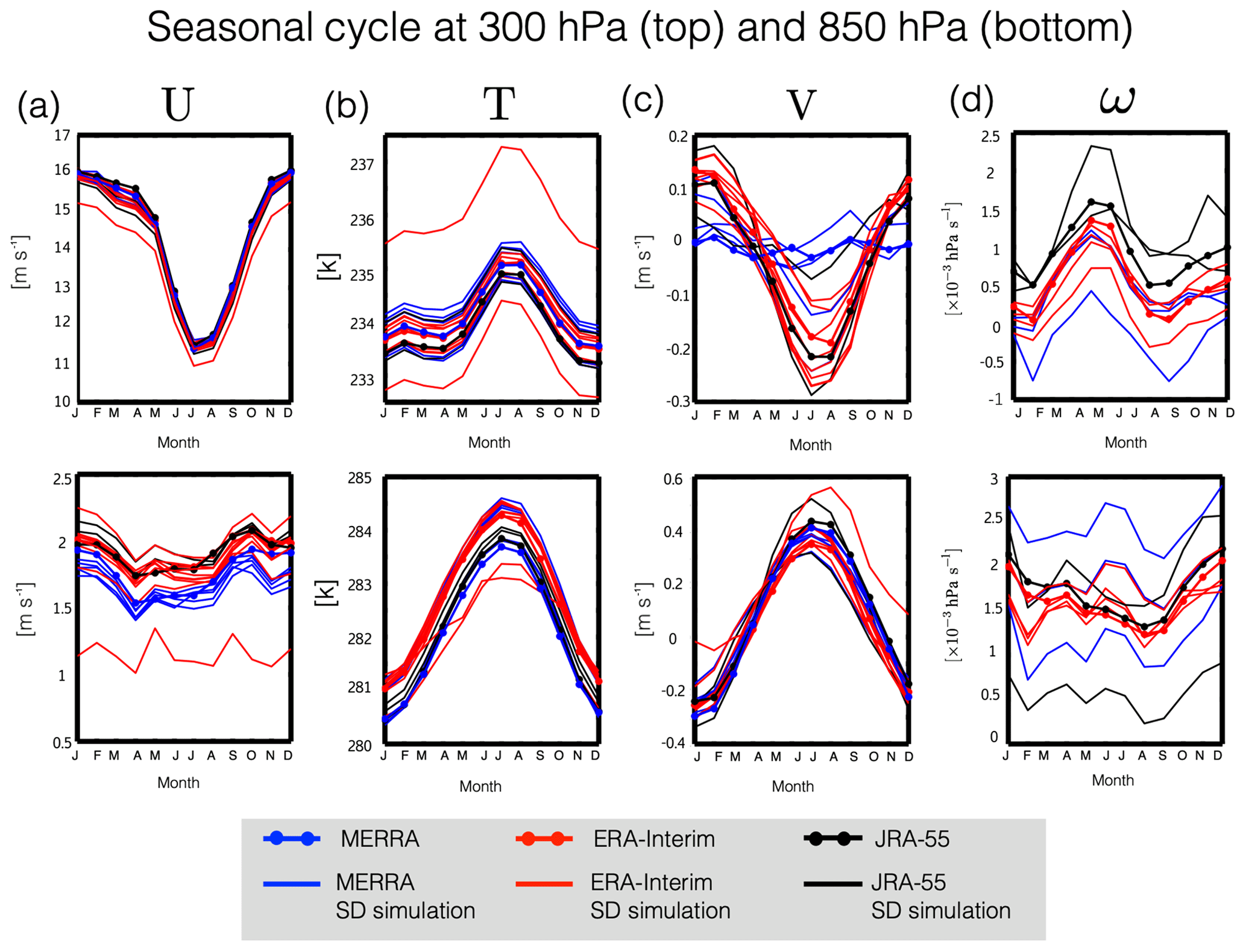
Figure 3 The 2000–2009 climatological mean seasonal cycle of the (a) zonal mean zonal wind (U), (b) zonal mean temperature (T), (c) zonal mean meridional wind (V), and (d) zonal mean pressure velocity (ω) at 300 hPa (top panels) and 850 hPa (bottom panels). Seasonal cycles have been averaged over latitudes spanning 60^∘ S and 60^∘ N (30^∘ S and 30^∘ N for ω). Red/blue/black solid lines correspond to SD simulations constrained with ERA-Interim/MERRA/JRA-55 reanalysis fields. Red/blue/black dotted lines correspond to the raw ERA-Interim/MERRA/JRA-55 meteorological fields. As in Fig. 1 note that MERRA assimilated fields are shown, for which ω is not available.

The seasonal cycle of U (Fig. 3a) agrees well among the SD simulations in both the upper and lower troposphere, with the exception of one outlier at 850 hPa. Closer inspection reveals that this particular ERA-I-constrained simulation (i.e., UMUKCA-SD) corresponds closely to the free-running simulation produced using the same model, suggesting that its difference from the SD ensemble primarily reflected biases in its underlying free-running model (Fig. S3; Table S3 in the Supplement, row 3). Comparisons of the seasonal cycle of the temperature, meridional winds and vertical winds also show generally good agreement among the SD simulations (Fig. 3b–d) in terms of the seasonal cycle phase (Fig. 4b–d, f–h, left), although the differences in phase for some variables are noticeably larger than for others. For example, the spread in τ_min for ω_850 hPa and in τ_max for V_300 hPa (Fig. 4b, left) is much larger than for the other fields. For the former case, this most likely reflects the fact that the seasonal cycle is not well defined over this latitudinal range and pressure level as there are two apparent minima occurring in both February and September (Fig. 3d, bottom). By comparison, for the latter case (V_300 hPa) the differences in the seasonal cycle phase largely reflect differences among the reanalysis products, with MERRA exhibiting a much weaker seasonal cycle, relative to both ERA-I and JRA-55 (Fig. 3c, top) (Table 3, row 1).

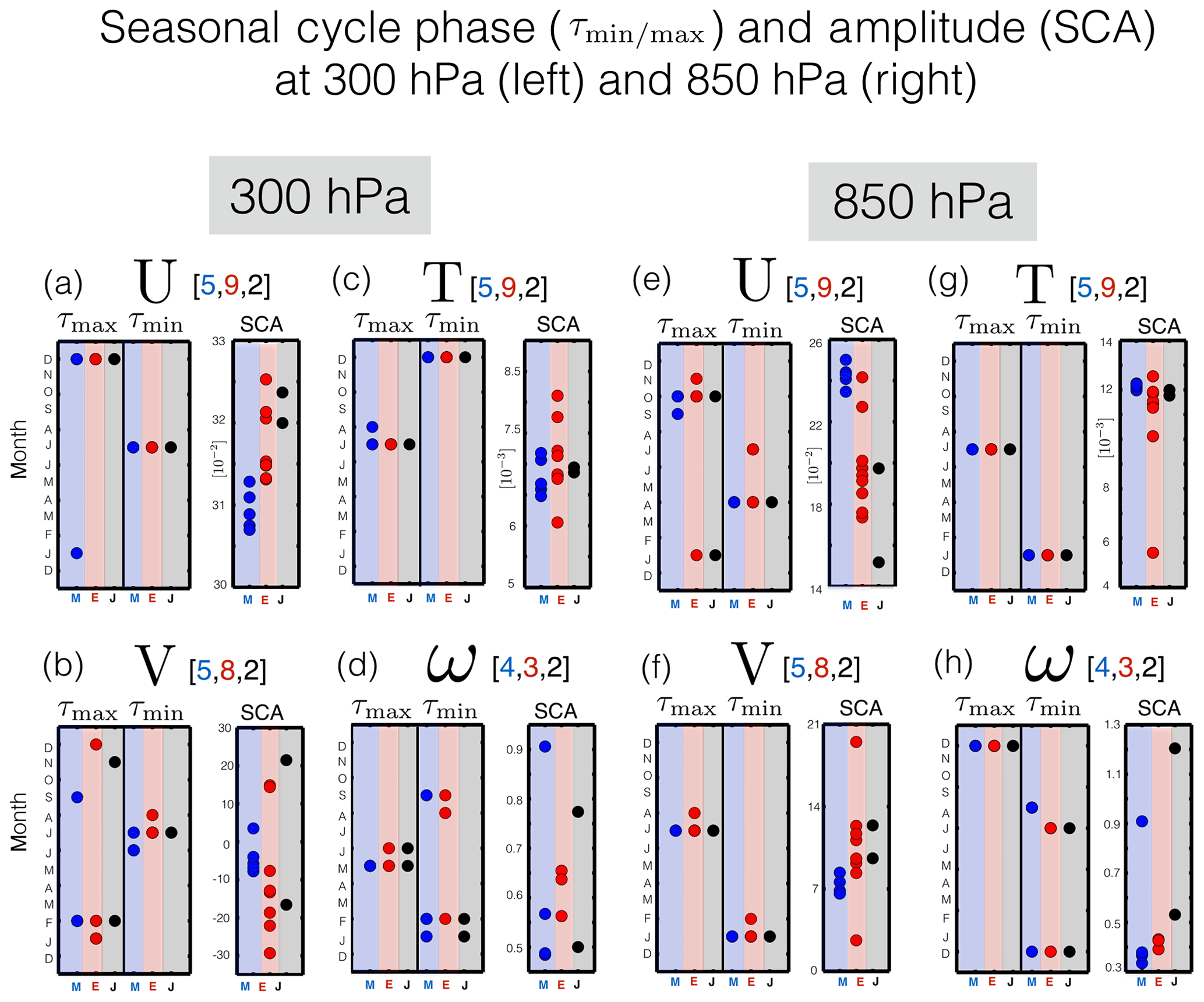
Figure 4 The seasonal cycle phase, represented in terms of τ_min and τ_max, and seasonal cycle amplitude (SCA) of the zonal mean zonal winds (a, e), zonal mean temperatures (c, g), zonal mean meridional winds (b, f) and zonal mean pressure velocities (d, h). Each dot represents an individual model simulation. The seasonal cycle amplitude has been normalized by the climatological mean annually averaged value for each variable shown. Red/blue/black circles show the spread among the SD simulations constrained with ERA-I/MERRA/JRA-55 reanalysis fields. Panels (a–d) and (e–h) correspond to evaluations at 300 and 850 hPa, respectively. Note that the number of ensemble members per ensemble and for each variable are shown in the title within each panel. In addition, note that in several panels only a few dots are visible. This reflects the overall good consistency in the seasonal cycle phase among the simulations.

While the seasonal cycle phases of U, V, T and ω are relatively well constrained by the SD simulations there are larger differences in the seasonal cycle amplitude (Fig. 4e–h). This is especially true for the meridional winds at both 300 hPa (Figs. 3c and 4b, right) and 850 hPa (Fig. 4f, right) and for the vertical winds, for which the SCA magnitude is anywhere between 0.3 and 1.2 of the climatological mean value (Fig. 4d, right; Fig. 4h, right). Note that for the case of the former (V_300 hPa), part of this can be understood in terms of the use of different reanalysis products, with MERRA exhibiting a much weaker seasonal cycle in V_300 hPa, compared to both ERA-I and JRA-55. At the same time, however, Fig. 4b and f clearly show large differences among only the ERA-I-constrained (and MERRA-constrained) simulations, indicating that both factors (i.e., different reanalysis products and implementation differences) contribute to the spread among the SD ensemble. Finally, note that the large normalized SCA values for the meridional wind fields reflect the fact that both V_300 hPa and V_850 hPa transition from positive to negative during the course of the annual cycle, which renders the annual climatological mean much smaller than the (unnormalized) SCA amplitude. For these two cases, therefore, the normalization of the SCA is somewhat less meaningful as a measure of seasonality, compared to the other variables.

Figure 5 Same as Fig. 3 but now for the stratospheric dynamical and transport diagnostics. Shown are the 2000–2009 climatological mean seasonal cycles of the (a) residual mean meridional velocity (v^*), (b) residual mean vertical velocity (w^*), (c) ozone (O₃), (d) nitrous oxide (N₂O), (e) stratospheric mean age (Γ_STRAT) and (f) NH midlatitude mean age (Γ_NH). The seasonal cycle is shown at 30 hPa (top panels) and 80 hPa (bottom panels), and all latitudinal averages have been performed over 60^∘ S and 60^∘ N (30^∘ S and 30^∘ N for w^*). For the cases of v^* and w^* red/blue/black dotted lines correspond to the S-RIP TEM velocities derived from ERA-Interim/MERRA/JRA-55 meteorological fields.

Comparisons of the seasonal cycle of the TEM circulation and stratospheric tracers (Fig. 5) also show generally good agreement in terms of the seasonal cycle phase among the SD simulations (Fig. 6, left). The main exceptions are N₂O at both 30 and 80 hPa (Fig. 6d) and O₃ at 80 hPa (Fig. 6c, bottom), where ${\mathit{\tau }}_{min/max}$ varies widely across the simulations. As shown in Fig. 5, this most likely reflects the fact that the seasonal cycle of these species is not well defined over this latitudinal and pressure range, indicating that care needs to be taken when interpreting ${\mathit{\tau }}_{min/max}$ since even subtle differences may manifest as large differences in the seasonal cycle phase.

Figure 6 Same as Fig. 4 but now for the stratospheric dynamical and transport diagnostics.

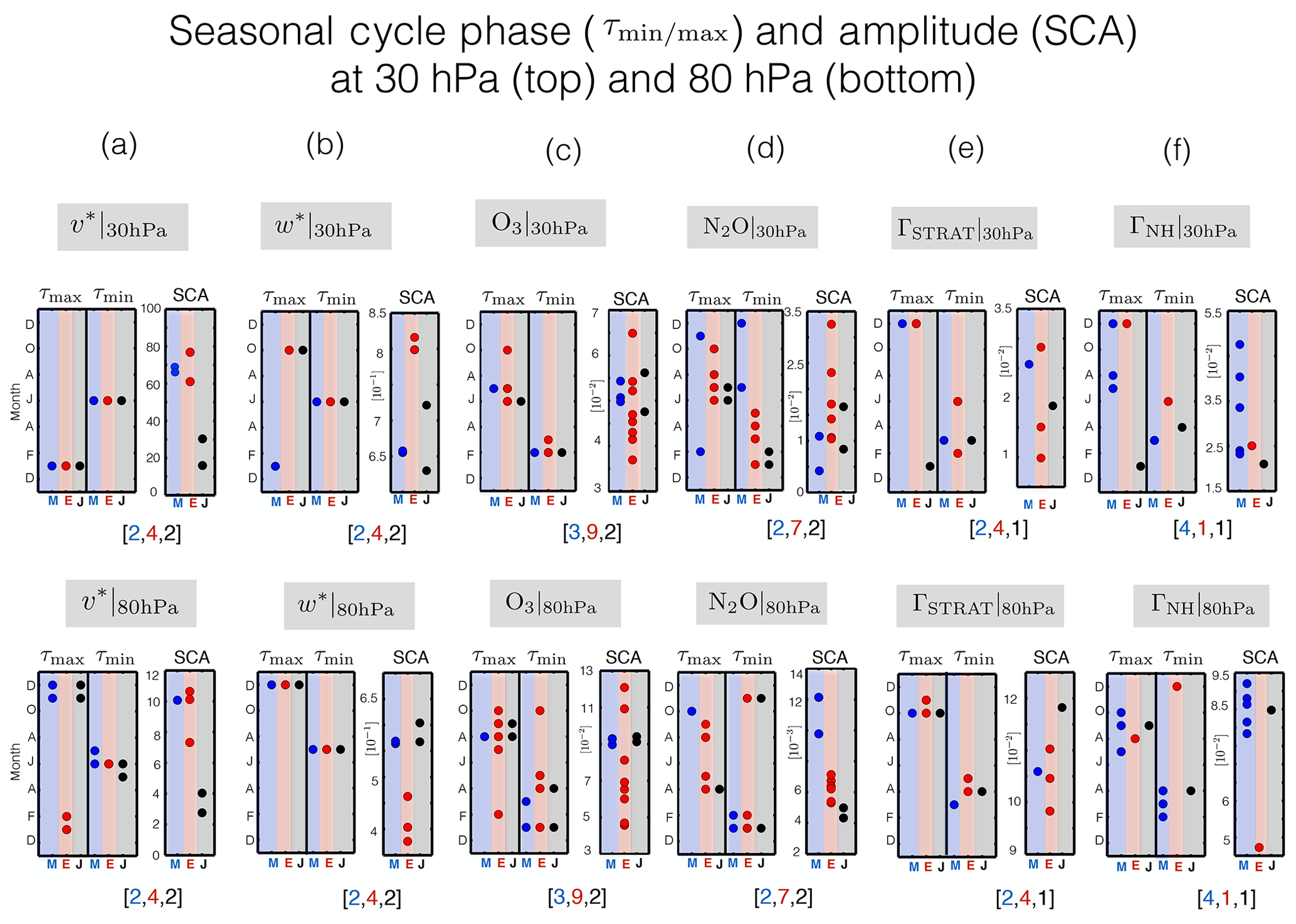
Similar to the tropospheric flow measures, the differences in SCA among the stratospheric transport and dynamical quantities are relatively larger, especially for $v_{\mathrm{80}\mathrm{hPa}}^{*}$ (Fig. 6a, bottom right) and for $w_{\mathrm{30}\mathrm{hPa}}^{*}$ (Fig. 6b, top right). The differences in SCA among the chemical and idealized tracers are also large (Fig. 6c–f, right) and, as in the troposphere, appear to be primarily associated with implementation differences and not with underlying differences among the reanalysis products. Furthermore, an additional comparison of the TEM and stratospheric tracer SD output with that from corresponding free-running simulations (not shown) reveals no systematic relationship between the SD ensemble biases and underlying free-running model biases (Table 3, row 3). Therefore, this indicates that the implementation of nudging is the largest source of spread in SCA for the stratospheric metrics considered here. Finally, given the fact that the seasonal cycle is not always well defined for all variables, we have checked the sensitivity of our calculations to the choice of latitudinal bounds over which the different fields were averaged before evaluating the seasonal cycle phase and amplitude. A discussion of these sensitivities is presented at the end of Sect. 5.

4.2.2 Interannual variability

We now extend our analysis to interannual timescales over the period 1980–2009. Deseasonalized time series of annual mean U, T, V and ω, averaged over 60^∘ S to 60^∘ N (30^∘ S to 30^∘ N for ω), covary well among the SD simulations (Fig. 7). Specifically, for U the average correlation coefficient among simulations in the SD ensemble (${\stackrel{\mathrm{‾}}{\text{corr}}}_{U,\text{SD}}$) is 0.97 at 300 hPa and 0.93 at 850 hPa (Table 4, column 2). The correlations in zonal wind among simulations within each analysis ensemble are also high, consistently exceeding 0.93 (Table 4, columns 3–5). Like the zonal winds, the temperature fields also covary well in the SD ensemble, with correlation coefficients of 0.95 (300 hPa) and 0.83 (850 hPa). Evaluating the covariability among the different analysis ensembles reveals that the somewhat poorer correlation values for T in the lower troposphere reflect differences among the ERA-I simulations, which have a correlation coefficient of 0.7 (Table 4). Closer inspection reveals that this is due to three of the ERA-I simulations (i.e., CHASER, IPSL and UMUKCA) and is consistent with the fact that the CHASER-SD simulation applied a much longer nudging timescale for T, compared to U and V (7 d vs. 0.8 d), while UMUKCA was nudged to U, V and θ but not explicitly to T. The covariability in the meridional winds (Fig. 7c) and vertical winds (Fig. 7d) is weaker than for the zonal winds and temperatures, although overall they are generally strong (>0.7). In some cases these weaker correlations are related to differences in covariability among the reanalysis products, as for the case of V_300 hPa, where the variability differs between MERRA and ERA-I, particularly over the period 1992–2002 (Fig. 7c, left; Table 3, row 3).

Table 4 Correlation coefficients for each variable χ among the SD, MERRA, ERA-Interim, JRA-55, SD^* and FR ensembles. Note that the SD^* ensemble consists only of those SD simulations for which there was also a corresponding FR simulation. Specifically, for the SD ensemble corr(i)_χ,SD corresponds to the correlation coefficient between the ith member time series of variable χ and the SD ensemble mean time series. Averaging over all SD ensemble members we have ${\stackrel{\mathrm{‾}}{\text{corr}}}_{\mathit{\chi },\text{SD}}\equiv \frac{\mathrm{1}}{N}{\sum }_{i=\mathrm{1}}^N\text{corr}(i{)}_{\mathit{\chi },\text{SD}}$. For all variables, correlations were evaluated over years 1980–2009. Bold values denote the coefficients for the main SD, SD^* and FR ensembles.

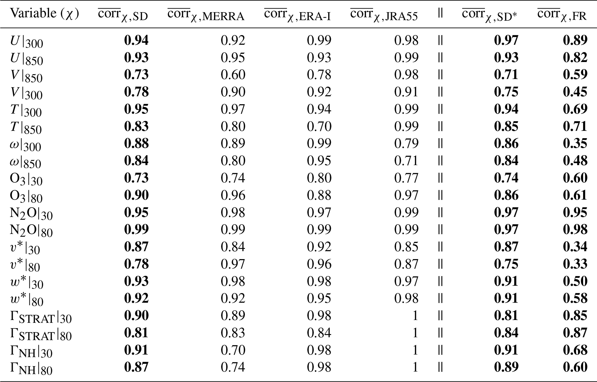
Figure 7 Time series of the zonal mean zonal winds (a), zonal mean temperatures (b), zonal mean meridional winds (c), and zonal mean vertical velocities (d) at 300 hPa (left panels) and 850 hPa (right panels). Red/blue/black solid lines correspond to SD simulations constrained with ERA-Interim/MERRA/JRA-55 reanalysis fields. Red/blue/black dotted lines correspond to the raw ERA-Interim/MERRA/JRA-55 meteorological fields. MERRA assimilated fields are shown for all variables, except for ω, for which output was not available.

Moving next to the stratosphere we also find generally strong correlations among time series of v^* and w^*, with values of ${\stackrel{\mathrm{‾}}{\text{corr}}}_{v^{*},\text{SD}}$ equal to 0.87 and 0.78 at 30 and 80 hPa, respectively, and ${\stackrel{\mathrm{‾}}{\text{corr}}}_{w^{*},\text{SD}}$ equal to 0.93 and 0.92 (also at 30 and 80 hPa) (Fig. 8 a,b). The weaker correlation coefficient associated with ${\stackrel{\mathrm{‾}}{\text{corr}}}_{v^{*},\text{SD}}$ at 80 hPa appears to be associated with the use of different reanalysis products, especially during years 1994–2000, where the ERA-I-constrained simulations exhibit a sharp decrease, which is not reflected either in the JRA-55 or MERRA simulations (Fig. 8a, right; Table 3, row 1). Among the constituents the correlations are relatively weaker although still generally strong, with positive correlations among simulations of ozone (${\stackrel{\mathrm{‾}}{\text{corr}}}_{{\mathrm{O}}_{\mathrm{3}},\text{SD}}=\mathrm{0.73}$ at 30 hPa and 0.90 at 80 hPa) and N₂O (${\stackrel{\mathrm{‾}}{\text{corr}}}_{{\mathrm{N}}_{\mathrm{2}}\mathrm{O},\text{SD}}=\mathrm{0.95}$ at 30 hPa and 0.99 at 80 hPa). (Note that the higher correlations in N₂O partly reflect the underlying positive multidecadal trend). The age correlations are also strong, all exceeding 0.81. When evaluating the covariability among the age tracers we did not include the results from the GEOS replay and WACCM-5hr simulations since those tracers were integrated with initial conditions that were not spun up, consistent with the description in Orbe et al. (2017b), whose comparisons focused on 2000–2009 climatological means. Therefore, given that those tracers do not equilibrate until the year ∼2000 we did not include them in our correlation analysis. Finally, as with our seasonal analysis, we have evaluated the sensitivity of our correlation analysis to the choice of spatial averaging; both sensitivity analyses are presented in Sect. 5.

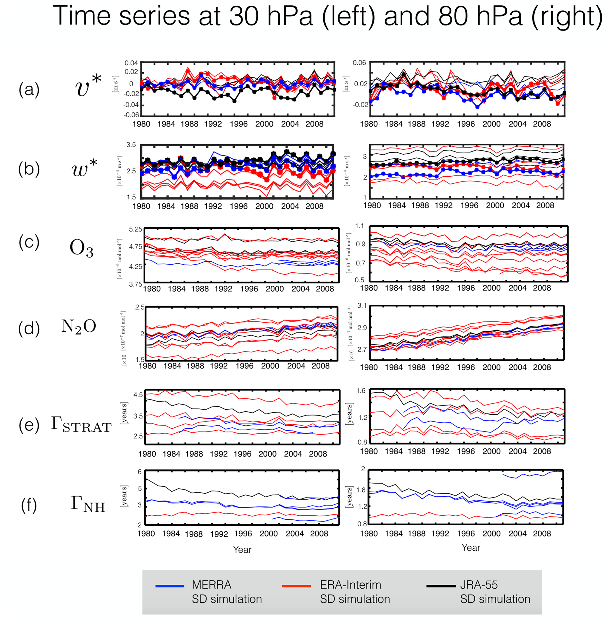
Figure 8 Same as Fig. 7 but for the stratospheric dynamical and transport fields, evaluated at 30 hPa (left) and 80 hPa (right). For the cases of v^* and w^* red/blue/black dotted lines correspond to the S-RIP TEM velocities derived from ERA-Interim/MERRA/JRA-55 meteorological fields.

4.2.3 Trends

To conclude this section we now briefly comment on trends, as inferred by simply taking the linear fits of the time series shown in Figs. 7 and 8 over the period 1980–2009. For the tropospheric dynamical measures U, V, T and ω, the trends exhibited by the SD simulations are in some cases in good agreement with the trends in the corresponding reanalyses (e.g., U₃₀₀, Fig. 9a, left). More generally, however, there is a large spread in the trends exhibited by the ERA-I ensemble, especially for the case of the meridional winds. As noted several times earlier this discrepancy is somewhat surprising given that V was explicitly constrained in all of the SD simulations.

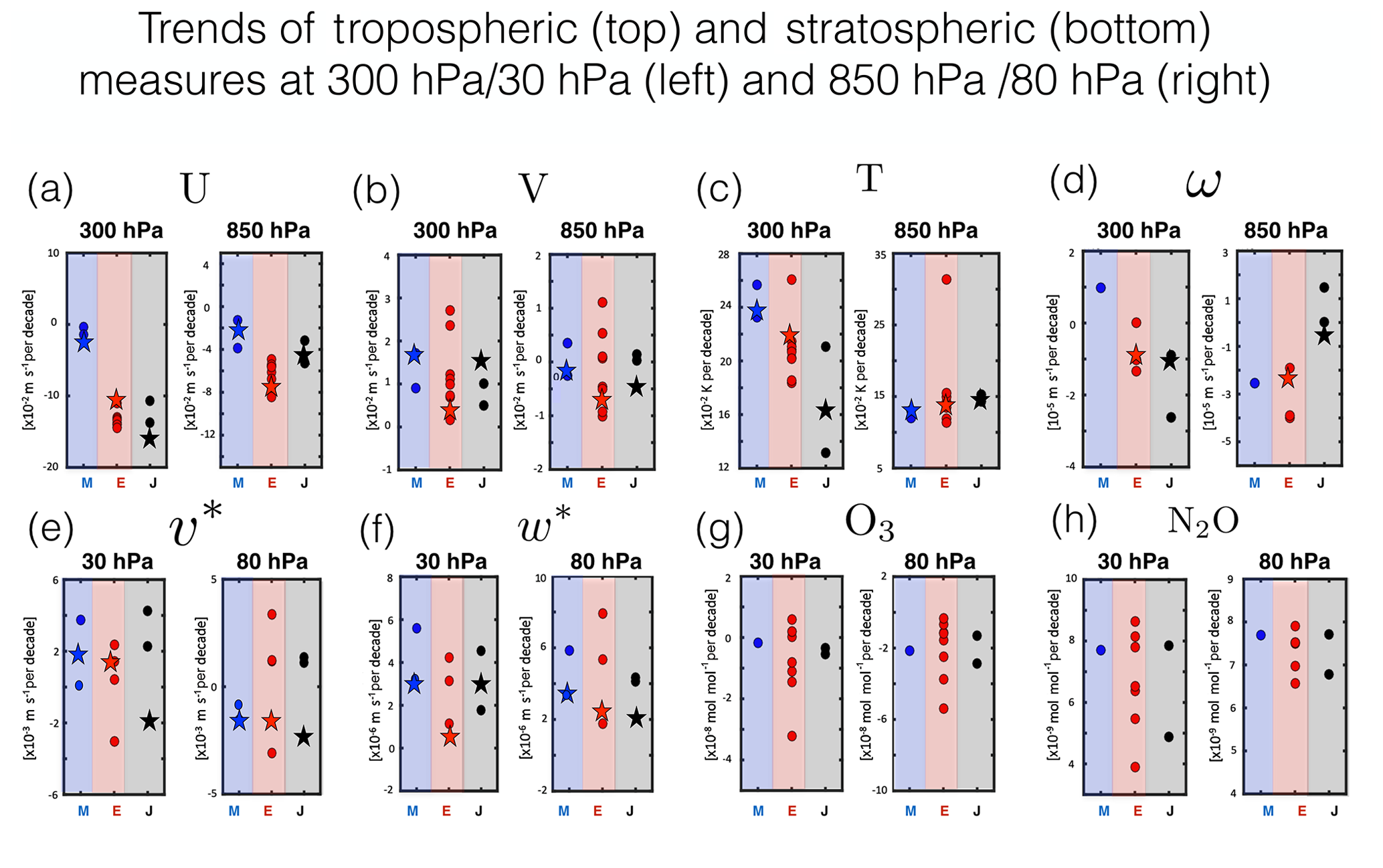
Figure 9 Top: trends in the zonal mean zonal winds (a), meridional winds (b), temperatures (c) and pressure velocities (d), evaluated as simple linear fits of the time series shown in Fig. 7 over years 1980–2009. Bottom: same but for the (e) residual mean meridional velocity, (f) residual mean vertical velocity, (g) ozone and (h) nitrous oxide. Red/blue/black circles denote the SD simulations, whereas the stars refer to the trends inferred directly from the S-RIP TEM velocities derived from ERA-I/MERRA/JRA-55 reanalysis fields.

In the stratosphere the spread in the trends is also large and, for the cases of v^* and w^*, larger than the spread in the trends exhibited by the reanalyses themselves (Fig. 9e–g). This latter point is consistent with Chrysanthou (see their Fig. 11c), who showed that the trends in the tropical upward mass flux in nudged CCMI simulations generally did not match those from the reanalyses to which they were nudged. Similar behavior is exhibited by the age tracers (not shown). While the trends in the constituents (i.e., ozone and nitrous oxide) generally agree in sign (negative and positive, respectively), the source of this agreement is likely driven by consistent variations in their sources and sinks and not by consistent underlying dynamical trends.

5 Free-running vs. specified-dynamics simulations

5.1 Climatology

In the previous section we showed that certain aspects of the SD simulations (e.g., seasonal cycle phase, interannual variability) appeared to be much better constrained compared to others (e.g., climatological means, seasonal cycle amplitude), relative to both the SD ensemble mean and the different reanalysis products. We now place these results in a broader context by comparing the SD simulations relative to free-running simulations produced using the same underlying models. To this end, therefore, we focus only on the subset of the SD simulations for which modelers also submitted a corresponding free-running simulation (column 4, Table 1), designated throughout as the SD^* ensemble. Thus, in this section we focus on how well the SD^* ensemble performs relative to FR ensemble, both of which consist of the same number N of ensemble members. Note that for cases where multiple nudged simulations were submitted (e.g., WACCM-5hr and 50-hr simulations) we only use one (in this case WACCM-50hr) to ensure that both the SD^* and FR ensembles have the same number of members.

Calculations of the root-mean-square (rms) spread reveal interesting differences between the SD^* and FR ensembles (Fig. 10). Specifically, for a given variable χ the rms spread for the N-member SD^* multimodel ensemble is defined at each pressure level and latitude as follows: $\stackrel{\mathrm{‾}}{\text{rms}}{}_{\mathit{\chi },{\text{SD}}^{*}}\equiv \sqrt{\frac{\mathrm{1}}{N}{\sum }_{i=\mathrm{1}}^N\left(\mathit{\chi }\right(i)-{\stackrel{\mathrm{‾}}{\mathit{\chi }}}_{{\text{SD}}^{*}}{)}^{\mathrm{2}}}$. Similarly, $\stackrel{\mathrm{‾}}{\text{rms}}{}_{\mathit{\chi },\text{FR}}$ refers to the rms spread averaged over the (also N-member) FR ensemble. Comparisons of $\stackrel{\mathrm{‾}}{\text{rms}}{}_{U,{\text{SD}}^{*}/\text{FR}}$ and ${\stackrel{\mathrm{‾}}{\text{rms}}}_{T,{\text{SD}}^{*}/\text{FR}}$ reveal that throughout the depth of the troposphere the zonal winds and temperatures are more consistent among the SD simulations, relative to the free-running models (Fig. 10a and c). By comparison, throughout the troposphere the values of ${\stackrel{\mathrm{‾}}{\text{rms}}}_{V,{\text{SD}}^{*}}$ and ${\stackrel{\mathrm{‾}}{\text{rms}}}_{V,\text{FR}}$ (Fig. 10b) are nearly identical, while, for the vertical winds, the spread among the SD^* ensemble is systematically larger than among the FR ensemble by ∼20 % (Fig. 10d). This suggests that nudging actually produces larger intermodel differences in the vertical winds, relative to those associated with underlying free-running model biases. While it is true that the vertical component of the wind field is not a prognostic variable (and, hence, not directly nudged), the larger spread in ω among the SD ensemble is, at the very least, surprising.

The rms spread comparisons of the stratospheric circulation and transport measures reveal a similar story, with similar values of v^*, w^*, and O₃ (Fig. 10e, f and g) among both the SD^* and FR ensembles. In the middle and upper stratosphere the rms spread is consistently greater in the SD ensemble for both N₂O (Fig. 9h) and Γ_STRAT (Fig. 9i). Interestingly, the rms comparisons of the age tracers do not produce a consistent story above 50 hPa, which, upon first glance, seems contradictory. However, as discussed earlier, this is because the SD ensembles for Γ_STRAT and Γ_NH consist of very different models. Specifically, the SD models included in the comparisons of Γ_NH include three MERRA-constrained simulations performed using models from the same modeling center (WACCM-5hr, WACCM-50hr, CAM). Therefore, the smaller rms spread for that tracer in the SD^* ensemble needs to be interpreted with caution, as it reflects similarities among three simulations produced using the same (or very similar) underlying model.

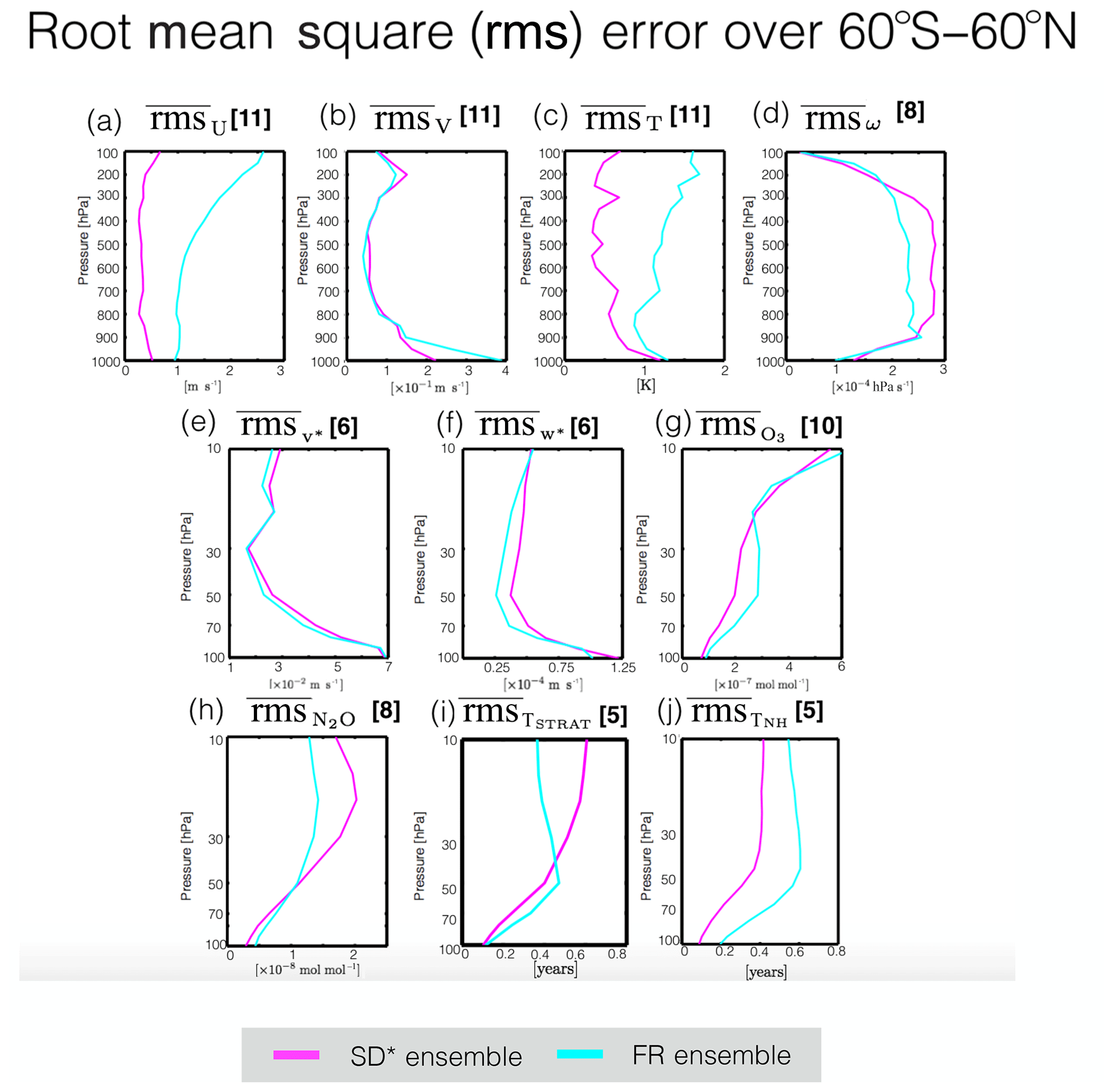
Figure 10 The root-mean-square (rms) spread of the (a) zonal mean zonal winds, (b) zonal mean meridional winds, (c) zonal mean temperatures, (d) zonal mean pressure velocities, (e) residual mean horizontal velocity, (f) residual mean vertical velocity, (g) ozone, (h) nitrous oxide, (i) stratospheric mean age and (j) NH midlatitude mean age. The pink and cyan lines correspond to the ensemble mean rms spread evaluated over the SD^* and FR ensembles, where the asterisk denotes the subset of SD simulations for which there was a corresponding free-running simulation (last column in Table 1).

Finally, as discussed earlier our decision to average over 60^∘ S and 60^∘ N may mask potentially interesting regions of rms spread that are smoothed out upon averaging and/or may raise concerns about the robustness of our conclusions. Therefore, we also compared the pressure and meridional distributions of the rms spread between the SD^* and FR ensembles (Figs. S4 and S5 in the Supplement). Overall, the rms patterns reflect the underlying structure of the model field such that regions of strong spatial gradients and/or reversals in sign tend to align with regions where the rms spread is larger. This applies to both SD^* and FR ensembles, with the exception of U, for which the rms values in the SD^* ensemble are negligible throughout the troposphere. While these patterns are interesting, they are more or less symmetric about the Equator, indicating that the use of a 60^∘ S and 60^∘ N averaging operator does not pose any obvious concerns regarding robustness of our results. Furthermore, for certain variables the rms spread exhibits strong vertical gradients (e.g., T, V) that support our use of 300 and 850 hPa and 30 and 80 hPa as representative pressure levels in the troposphere and stratosphere, respectively.

5.2 Variability

Comparisons of the seasonal cycle among the SD^* and FR ensembles (Fig. 11) show that the seasonal cycle phase is generally more consistent among the SD^* simulations, compared to the FR simulations, although there are cases where the differences in phase spread among the ensembles are similar (e.g., ω and V in Fig. 11b, d, f and h, left). The seasonal cycle amplitude is also somewhat better constrained in the SD^* ensemble, at least for U and T. However, there are large differences in SCA amplitude in the meridional and vertical winds, evident in both the lower and upper troposphere (Fig. 11b, d, f and h, right).

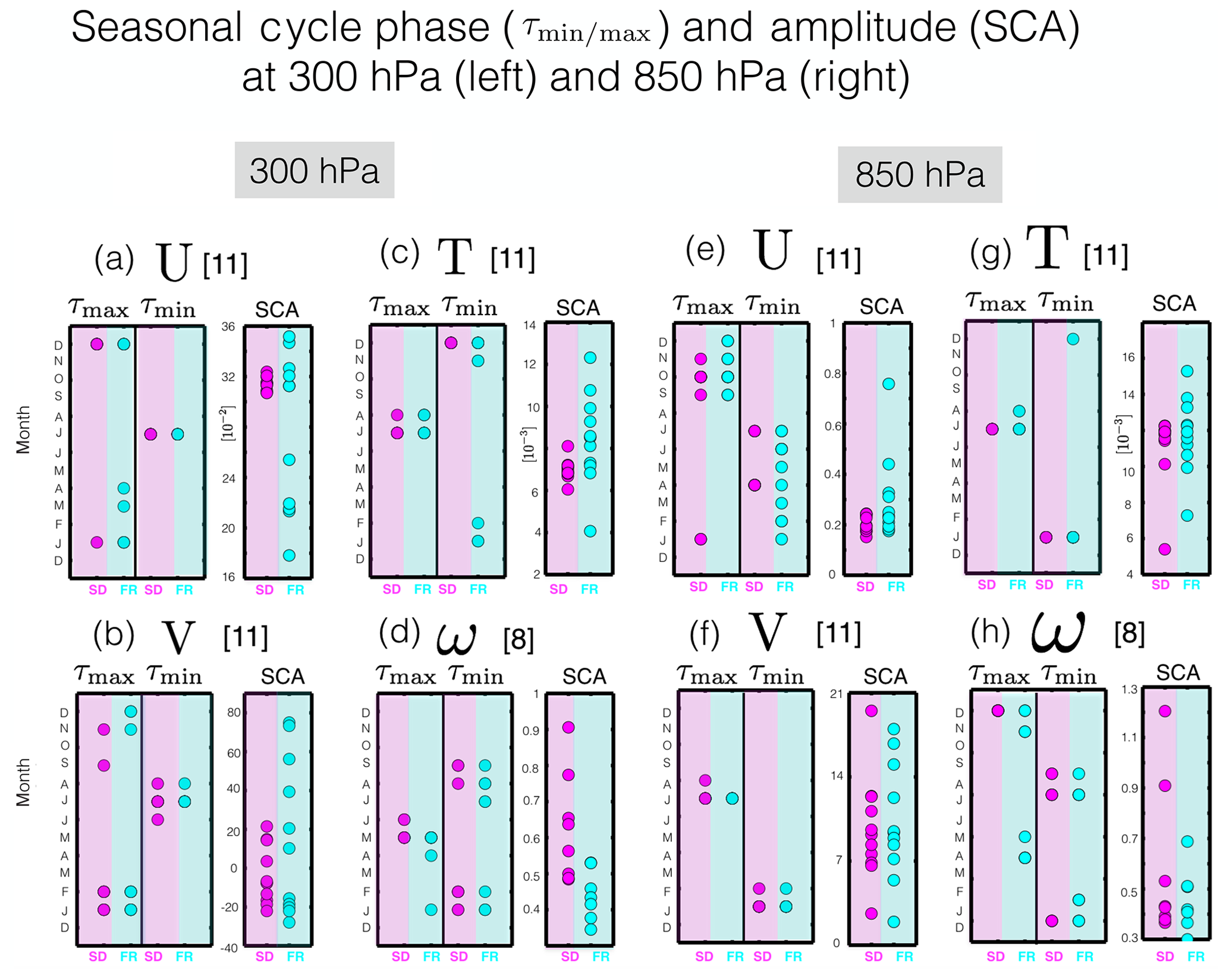
Figure 11 Same as Fig. 4 but now evaluated for the SD^* and FR ensembles in pink and cyan, respectively. Note that both ensembles contain the same number of ensemble members per variable, as shown in the title within each panel.

The seasonal cycle phase of the TEM and transport circulations appears to be slightly better constrained among the SD^* vs. FR ensembles (Fig. 12, left). As with the other variables, however, the seasonal cycle amplitude is, by comparison, less well constrained in both SD^* and FR ensembles. Specifically, at 80 hPa the seasonal cycle amplitude differences among the SD^* runs are larger than among the FR models for the cases of v^* at 80 hPa (Fig. 12a, bottom), w^* at 80 hPa (Fig. 12b, bottom), O₃ at 80 hPa (Fig. 12c, bottom), N₂O at 30 hPa (Fig. 12d, top) and Γ_STRAT at 30 hPa (Fig. 12e, top). Overall, upon comparing ensembles of equal sizes, we conclude that, while the seasonal cycle phase is slightly better constrained in the SD^* ensemble, the amplitude is not.

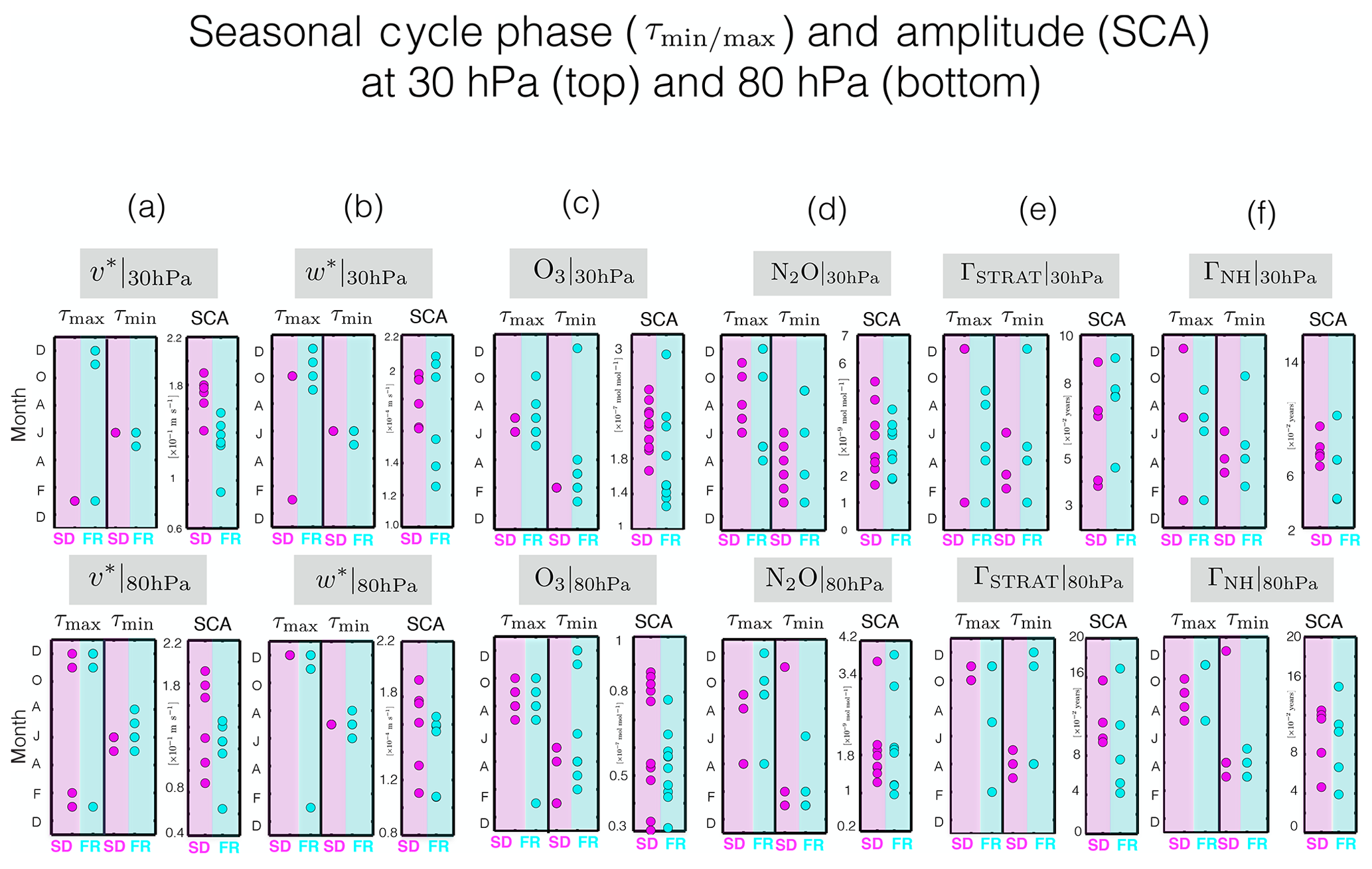
Figure 12 Same as Fig. 11 but now evaluated for the stratospheric dynamical and transport variables, shown here at 30 hPa (top) and 80 hPa (bottom).

As with our analysis of the rms spread, we have also checked the sensitivity of our seasonal cycle calculations to the choice of latitudinal averaging bounds. As indicated earlier in Sect. 4, in a few cases the seasonal cycle was either too small in amplitude or not characterized by a unique maximum/minimum, which raised questions about the appropriateness of the SCA and ${\mathit{\tau }}_{min/max}$ diagnostics. Therefore, in addition to that analysis we have evaluated the correlation of the seasonal cycle at each grid point for each member of both the SD^* and FR ensembles, relative to the SD^* and FR ensemble averages, respectively. Figures S6 and S7 in the Supplement show that for U, V, T and ω the SD ensemble shows overall high correlations over all levels and latitudes, except for the tropical midtroposphere between 300 and 700 hPa for V, where the meridional winds transition in sign from mean southerly/northerly flow; in this latter case the low correlation coefficients therefore most likely reflect differences between small numbers. For the TEM variables there is also an interesting spatial structure in the correlations of v^* and w^* for the SD^* ensemble, with relatively lower correlations in the lower and middle stratosphere, and for N₂O, with relatively lower correlations over the NH middle and high latitudes for both SD and FR ensembles. Overall, however, the spatial patterns of correlation coefficients for all variables are more or less symmetric about the Equator and span much of the subtropics and extratropics within our latitudinal averaging bounds. Therefore, while this spatial structure is interesting on a case-by-case basis, we feel that the use of 60^∘ S to 60^∘ N (30^∘ S to 30^∘ N for ω and w^*) latitude averaging bounds is appropriate for synthesizing our results and does not hinder the robustness of our conclusions.

Comparisons of the rms spread between the FR and SD^* ensembles (Table 4, last two columns) reveal that the SD simulations nearly always exhibit much more consistent interannual variability, compared to their free-running counterparts. This is particularly clear for the meridional winds in the upper troposphere (300 hPa), where ${\stackrel{\mathrm{‾}}{\text{corr}}}_{V,{\text{SD}}^{*}}=\mathrm{0.75}$, compared to ${\stackrel{\mathrm{‾}}{\text{corr}}}_{V,\text{FR}}=\mathrm{0.45}$. Similarly, the vertical velocity interannual variability is much better constrained in the SD^* ensemble, with ${\stackrel{\mathrm{‾}}{\text{corr}}}_{\mathit{\omega },{\text{SD}}^{*}}$ = 0.86 compared to ${\stackrel{\mathrm{‾}}{\text{corr}}}_{\mathit{\omega },\text{FR}}=\mathrm{0.35}$ at 300 hPa. The TEM circulation also covaries better among the SD simulations as do ozone variations at both 30 hPa and 80 hPa, with correlation coefficients that are about 0.2 larger than for the FR simulations.

Figure 13 Same as Fig. 9 but now evaluated for the SD^* and FR ensembles in pink and cyan.

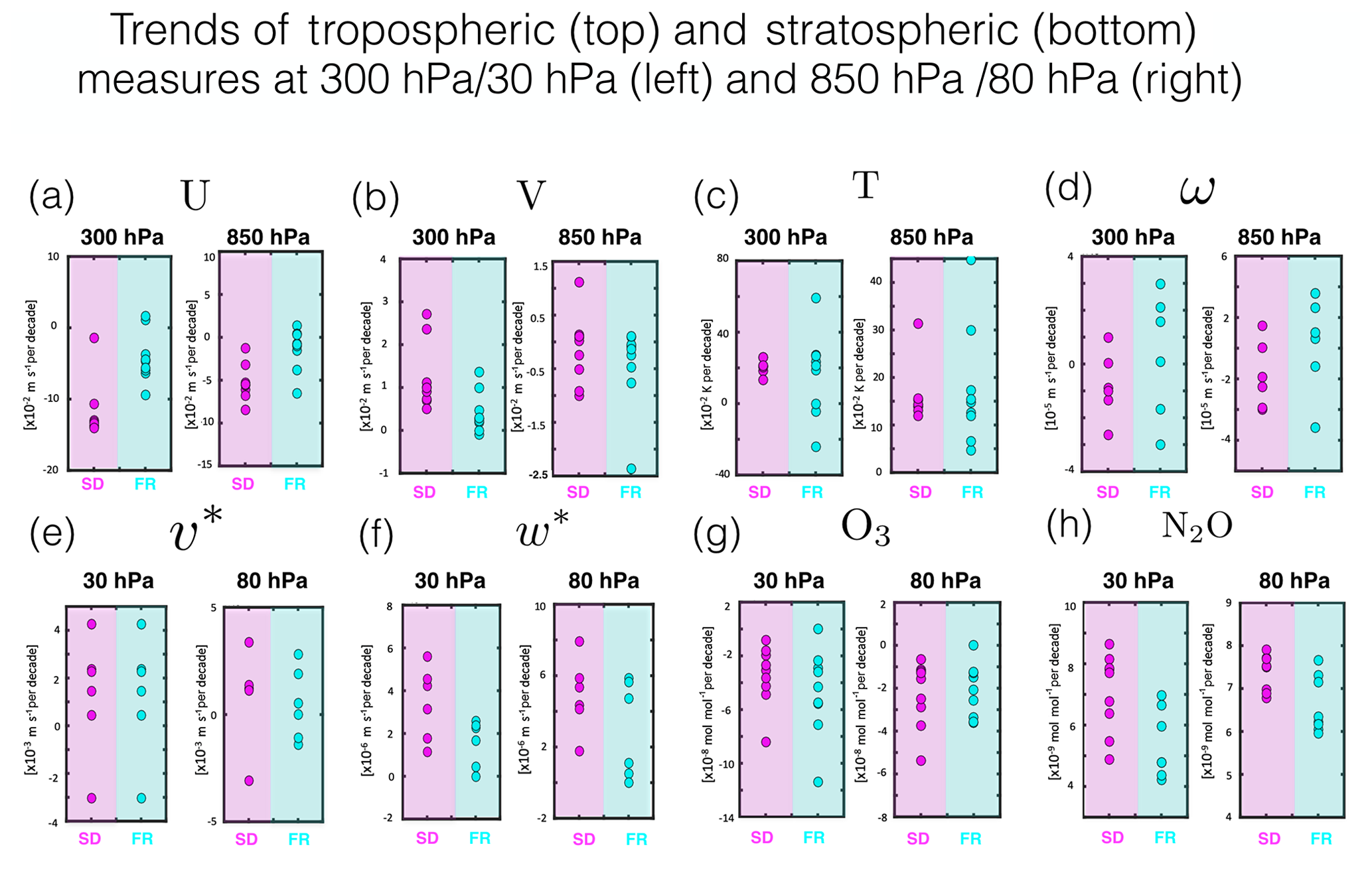
Finally, the trends simulated by the SD^* ensemble show a similar – if not larger – disagreement compared to the trends simulated by their corresponding FR models (Fig. 13). While for the cases of U, V and T (Fig. 13a–c) the spread in the SD^* simulated trends is somewhat smaller, this does not apply generally, especially for the cases of v^*, w^* and the constituents (Fig. 13e–g). Chrysanthou et al. (2019) came to a similar conclusion with respect to the tropical upward mass flux, which they showed exhibited larger trend discrepancies, compared to the free-running simulations (compare panel c in their Figs. 10 and 11). Large trend discrepancies in the tropical upward mass flux were also exhibited by the SD simulations, compared to the reanalyses (compare their Fig. 13 and supplementary Fig. 17).

5.3 Dynamical consistency

Whereas in the previous sections we evaluated the SD simulations in terms of their representation of individual fields, here we briefly examine the dynamical consistency of the large-scale circulation. Given the surprising differences in the tropospheric meridional winds we restrict our attention to the tropical mean meridional circulation and, in particular, to the Hadley cell (HC). Waugh et al. (2018) compared a broad range of lower and upper tropospheric measures of the HC and found that the strongest relationships occurred between the HC edge based on the near-surface zonal winds (hereafter denoted as UAS) and the HC edge based on the meridional mass streamfunction (hereafter PSI) among both reanalysis and free-running models from CMIP5 (Taylor et al., 2012). Furthermore, they showed that strong correlations between UAS and PSI occur not only on interannual timescales but also in terms of their trends and forced responses to global warming.

Figure 14 compares UAS and PSI among the SD^* and FR ensembles. Specifically, UAS corresponds to the first subtropical latitude where the near-surface zonal wind changes from negative to positive. By comparison, PSI corresponds to the zero-crossing of the meridional mass streamfunction (Ψ) at 500 hPa, where Ψ was calculated as the vertical integral of the meridional component of the zonal mean wind using the TropD software package from Adam et al. (2018). The comparisons of UAS and PSI first show that UAS is very well constrained in both hemispheres among the SD^* simulations, exhibiting a spread that is much smaller (∼1–2^∘), compared to their corresponding FR simulations (up to $\sim \mathrm{10}{}^{\circ }$) (Fig. 14a). By comparison, the spread in PSI is much larger, especially during boreal summer in the NH, where PSI differs by $\sim \mathrm{25}{}^{\circ }$ compared to a much smaller range among the FR simulations ($\sim \mathrm{10}{}^{\circ }$) (Fig. 14b). More importantly, the relationship between UAS and PSI is entirely different between the SD and FR ensembles. That is, consistent with Waugh et al. (2018), the FR simulations exhibit a strong positive relationship between UAS and PSI, especially in the SH, such that a more poleward UAS is associated with a more poleward PSI. This relationship is not demonstrated by the SD simulations, indicating that the meridional and zonal components of the flow are not dynamically consistent in that ensemble of runs, similar to the results presented in Davis and Davis (2018), although their focus was on the actual reanalysis fields (not nudged simulations).

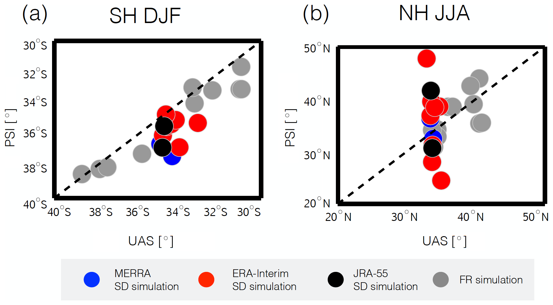
Figure 14 Correlations of PSI and UAS, two independent measures of the Hadley cell edge calculated from the meridional winds and zonal winds, respectively, evaluated over years 1980–2009 for both the SD^* and FR^* ensembles. Correlations are shown for SH DJF (a) and NH JJA (b), with red/blue/black circles corresponding to ERA-I/MERRA/JRA-55 simulations while grey circles denote free-running simulations.

6 Conclusions

The main goal of this study has been to document how the REF-C1SD experiment was implemented across the Chemistry-Climate Model Initiative (CCMI) models, since this information is not available in the published literature. While some of the information described here is addressed in supplementary Table 30 of Morgenstern et al. (2017), we have included a more complete description, based on information solicited from individual modeling groups in the form of a community survey. Furthermore, we have also used this opportunity to present a more rigorous evaluation of several dynamical and transport fields that were provided as output but were only briefly discussed in Orbe et al. (2018) and Yang et al. (2019). Our analysis has distinguished how well the specified-dynamics (SD) simulations represent climatologically averaged versus temporally varying zonal mean distributions with respect to the entire SD ensemble, reanalysis products and free-running simulations produced using the same underlying models. Our conclusions are summarized as follows:

• Comparisons of the climatological annually and zonally averaged zonal winds and temperatures show good agreement in the troposphere among the SD simulations and with respect to the reanalysis fields. By comparison, the differences in the meridional winds and vertical winds are much larger (∼30 %–40 %) and are related both to the use of different reanalysis products and to differences in implementation. In the stratosphere, the spread in the climatological transformed Eulerian mean (TEM) and transport circulations among the SD simulations is also large (approaching ∼100 %) and is primarily related to differences in implementation.

• For most variables (both tropospheric and stratospheric) there is good agreement (<20 % spread) in terms of the phase of the seasonal cycle; by comparison, the seasonal cycle amplitude (SCA) exhibits much larger differences (∼50 %). On interannual timescales, the SD simulations exhibit good covariability (correlation coefficients >0.7) for nearly all fields.

• Overall, the spread in both the mean climatological distributions and SCA among the SD simulations cannot be attributed solely to the use of different reanalysis products. While in some cases (e.g., V_300 hPa) the differences among the reanalysis products are large, in general the SD spread is much larger.

• For most variables the SD simulations perform similarly to – and in several cases (e.g., meridional winds, TEM circulation) worse than – free-running simulations produced using the same models in terms of their climatological mean values and seasonal cycle amplitudes. By comparison, the SD simulations consistently exhibit superior covariability on interannual timescales for nearly all variables analyzed here, although their trends differ substantially both with respect to each other and compared to their corresponding reanalyses, consistent with findings from previous studies.

• Interestingly, the relationship between the meridional and zonal components of the flow is fundamentally different between the SD simulations and the FR simulations. Unlike the free-running simulations, the specified-dynamics simulations do not exhibit a strong correlation between indices of the Hadley cell derived separately from the zonal vs. meridional winds. This reveals that different components of the flow are not dynamically consistent in all of the SD simulations.

We have shown that there are large differences in how SD simulations represent the mean climatological distributions and seasonal cycle phases of various tropospheric and stratospheric flow and transport measures. The differences in the meridional winds are particularly surprising, given that all simulations were explicitly constrained to meridional winds derived from the analysis fields. At the same time, we also showed that the SD simulations exhibit much better covariability on interannual timescales, relative to free-running simulations using the same underlying models. Note that, upon testing the sensitivity of our analysis to the choice of metrics, we found that for a few variables and locations the phase of the seasonal cycle was not well defined (e.g., N₂O), in which cases the spread in ${\mathit{\tau }}_{min/max}$ may be less meaningful. However, these cases were anomalies and, after redoing our analysis in terms of similar but distinct metrics (e.g., correlation of the seasonal cycle vs. SCA), we found qualitatively similar results supporting our original conclusions. In addition, we also found that our main conclusions were robust to how our calculations were performed, specifically with respect to the choice of both latitudinal averaging bounds and pressure levels.

Overall, our analysis suggests that studies using SD simulations should exhibit strong caution when inferring the influence of dynamics on tracers. More precisely, our results indicate that studies relating large-scale dynamics to atmospheric transport would be most justified in using SD simulations to examine science questions related to interannual variability; by comparison, studies would be less justified to address questions hinging on credible representations of the seasonal cycle amplitude, trends or the overall magnitude of the large-scale flow. The lack of dynamical consistency exhibited by some SD simulations, at least with respect to the tropospheric subtropical flow, also raises concerns that may complicate the interpretation of results using nudged simulations to study the influence of atmospheric dynamics on composition. Overall, several of our findings are consistent with the analysis in Chrysanthou et al. (2019), who provided a thorough comparison of the stratospheric residual mean circulation among the REF-C1SD simulations, but their analysis does not extend to stratospheric trace gases (or the troposphere). In the spirit of providing a review of the REF-C1SD experiment our focus here has been broader in scope.

An important conclusion from our analysis is that the differences among the SD simulations are not primarily driven by differences between the reanalysis fields. To this end we have attributed the SD ensemble spread primarily to differences in implementation. It is important to clarify, however, that by “implementation” we refer to both the departures from the analysis fields associated with nudging and biases associated with the underlying free-running models (Table 3, rows 2 and 3). Therefore, for those fields for which it was shown that outlier SD simulations closely tracked their corresponding free-running simulations, our conclusion is that the SD ensemble spread primarily reflects biases in the underlying free-running models (e.g., T_850 hPa). For other cases, however, in which the SD ensemble spread was shown to be larger than in the FR ensemble (e.g., $w^{*},\mathit{\omega },{\mathrm{N}}_{\mathrm{2}}\mathrm{O}$), we conclude that the act of nudging actually produces larger divergence among the models than would be expected solely due to underlying differences in model formulation. Furthermore, as discussed in Sect. 5, while the SD ensemble included results from three chemical transport models (CTMs), the majority of the simulations considered here were performed using nudged chemistry–climate models (CCMs). While we could not identify clear CTM vs. nudged differences in our analysis in Sect. 5, future studies should focus on more systematically comparing the performance of nudged simulations not only relative to free-running simulations, as examined here, but also relative to offline CTMs.

One final caveat of our analysis is that we have only compared the resolved large-scale flow. Therefore, when interpreting the transport differences, reflected in both the idealized and chemical tracers, one must also consider differences in transport related to subgrid-scale processes (e.g., parameterized convection, vertical diffusion) (Orbe et al., 2017a, 2018). In particular, Orbe et al. (2018) showed that the parameterized convection differences in the troposphere are even larger among the REF-C1SD simulations, relative to the REF-C1 ensemble, especially in the tropics. Our analysis here, therefore, has aimed solely at providing a more detailed description of the large-scale flow representation in the SD ensemble, compared to the briefer discussions presented in earlier works. Finally, the second assumption that we have made is that any inconsistencies related to the use of different advection schemes used for simulating the flow and tracers are small, relative to transport differences arising in response to how nudging is implemented among the various simulations. However, as noted in Morgenstern et al. (2017), only one of the CCMI models considered here (UMUKCA) uses different schemes for the advection of chemical vs. physical tracers (e.g., momentum, heat), indicating that our assumption is valid in the context of the larger SD ensemble.

Appendix A: Description of individual REF-C1SD simulations

A1 CESM1 CAM4-chem and CESM1 WACCM

The CAM4-chem and WACCM-5hr(50hr) REF-C1SD simulations are nudged to MERRA 6-hourly instantaneous analysis fields, applying a mass-conserving interpolation of the MERRA fields ($\mathrm{1}/\mathrm{2}{}^{\circ }$ latitude by $\mathrm{2}/\mathrm{3}{}^{\circ }$ longitude) to the models' horizontal grids (1.9^∘ latitude by 2.5^∘ longitude). Nudged meteorological fields include both three-dimensional fields (T, U, V) and the two-dimensional fields PS, TAUX and TAUY, SHFLX, and LHFLX (surface pressure, surface stress, latent heat flux and sensible heat flux). Note that water vapor is derived in the model. Nudging occurs over a 30 min time step and is applied linearly (in pressure) from the surface to 50 km, above which the simulation is fully free-running. The nudging relaxation time constant τ is spatially constant and set to 50 h⁻¹ (5 h for WACCM-5hr). Spectral nudging is not used.

In addition to being forced by SSTs and SICs from HadISST, the CAM4-chem and WACCM REF-C1SD simulations use PHIS (topography) from MERRA. Drifts in surface pressure that are generated by nudging are corrected for at every advection step (or every $\mathrm{30}\min /\mathrm{8}=\mathrm{3.75}\min$). The convective mass fluxes are not taken from MERRA but rather derived from CAM.4 column physics, which represents convection using the parameterizations of Zhang and McFarlane (1995) and Hack (1994) for deep and shallow convection, respectively.

Reference: Lamarque et al. (2013).

A2 CCSRNIES MIROC3.2

The CCSRNIES MIROC3.2 REF-C1SD simulation is nudged to 6-hourly ERA-I instantaneous fields and forced with prescribed HadISST1 boundary conditions. The analysis fields are linearly interpolated temporally to the model time and spatially interpolated linearly in the horizontal and linearly with respect to log-pressure levels in the vertical. The nudged three-dimensional meteorological fields are T, U and V using a nudging time step equal to the model time step for dynamics, and nudging is applied from the surface to 1 hPa. Above 1 hPa U and T are nudged to zonal mean fields obtained from CIRA (COSPAR International Reference Atmosphere), with no representation of year-to-year variability. The nudging relaxation time constant τ is set to a value of 24 h⁻¹ throughout the domain, and spectral nudging is not used. To correct for surface pressure drifts a pressure correction is applied. Convective mass fluxes are recalculated online using the parameterization described in Arakawa and Schubert (1974).

Reference: Akiyoshi et al. (2016).

A3 HadGEM3-ES

The HadGEM3-ES REF-C1SD simulation is nudged to ERA-I 6-hourly instantaneous fields and forced with HadISST1 SSTs. The analysis fields are linearly interpolated temporally to the model time step; spatially, bilinear interpolation is applied in the horizontal and linear (in log pressure) interpolation in the vertical. The three-dimensional fields T, U and V are nudged every model time step (i.e., every 20 min) to a value interpolated between the instantaneous fields valid at the previous and next 6 h slot (e.g., between data for 00:00 GMT and 06:00 GMT). While nudging is uniform at all levels between 2.5 and 50 km there is transition from 0 to full-strength nudging over the top and bottom levels of the nudging domain. Neither spectral nudging nor a pressure correction for surface pressure drifts is used. Moist convection is parameterized using Walters et al. (2014).

Reference: Hardiman et al. (2017).

A4 GFDL-AM3

The GFDL-AM3 REF-C1SD simulation is nudged to NCEP/NCAR T62 6-hourly instantaneous fields and constrained with HadISST2 SSTs. The NCEP reanalysis fields, which are at T62 horizontal resolution, are interpolated to the C48 native model cubed sphere grid (∼200 km by ∼200 km). Only the horizontal winds U and V are nudged using a nudging time step equal to the model time step (i.e., every 30 min). Nudging is pressure-dependent between the surface and 10 hPa, with τ=6 h in the surface level, and weakening linearly (in pressure) to 60 h at 100 hPa and 600 h at 10 hPa. Neither spectral nudging nor a pressure correction for surface pressure drifts is used. The convective mass fluxes are calculated online using the parameterization described in Donner et al. (2011).

References: Lin et al. (2012, 2014, 2015a, b).

A5 TOMCAT CTM

The TOMCAT CTM simulation is constrained using ERA-I 6-hourly instantaneous analysis fields which are interpolated linearly in time to the model time step (1 h). Horizontally, the vorticity, divergence, surface pressure and temperature fields are read in as spectral coefficients, and a spectral transform is applied, which averages those fields onto the model horizontal grid. Kinematic velocities are used in the vertical and are determined by reading the vorticity in every 6 h and using that to compute the vertical mass flux, which is distributed over the model levels in order to conserve total mass advection. The TOMCAT simulation is among a subset of the REF-C1SD simulations that are not forced with observed boundary conditions but, rather, SSTs and SICs taken from an old NCAR CCM-II model. Convective mass fluxes are calculated online using the moist convective mass flux scheme of Tiedtke (1989). The model has parameterizations for subgrid-scale tracer transport by convection (Stockwell and Chipperfield, 1999; Feng et al., 2011) and boundary layer mixing (Holtslag and Boville, 1993).

Reference: Chipperfield et al. (2006).

A6 IPSL LMDz-REPROBUS

The IPSL LMDz-REPROBUS REF-C1SD nudged simulation is constrained with ERA-I 6-hourly instantaneous fields and forced with SSTs and SICs from the AMIP II dataset. The nudged fields U, V and T are linearly interpolated spatially to the model grid and linearly interpolated temporally to the model time step (1∕2 h). Nudging occurs everywhere and operates on a timescale ranging up to 3 h, depending on altitude. Neither spectral nudging nor a pressure correction for surface pressure drifts is used. Convective mass fluxes are calculated online using the convection scheme of Dufresnes et al. (2013).

References: Marchand et al. (2012), Szopa et al. (2013) and Dufresne et al. (2013).

A7 CMAM-SD

The CMAM REF-C1SD simulation is nudged to ERA-I 6-hourly instantaneous fields and forced with HadISST1 boundary conditions. The three-dimensional meteorological fields are vorticity, divergence and temperature and are linearly interpolated vertically to the model grid and linearly interpolated temporally to the model time step (7.5 min). Spectral nudging is applied in the horizontal for all waves up to T21 (nudged with equal strength). While no interpolation is required in the horizontal, vertically the analysis fields are linearly interpolated to the model levels. Nudging occurs at every model time step using a timescale τ=24 h for all model levels up to 1 hPa, above which the model is free-running. No pressure correction is applied to correct for surface pressure drifts. The convective mass fluxes are recalculated online and parameterized using Zhang and McFarlane (1995).

References: Jonsson et al. (2004) and Scinocca et al. (2008).

A8 UMUKCA

The UMUKCA REF-C1SD simulation is nudged to ERA-I 6-hourly instantaneous fields and forced with HadISST SSTs and SICs. The three-dimensional nudged meteorological fields are U, V and θ and are linearly interpolated temporally to the model time step (20 min) and spatially to the $\sim \mathrm{2.5}{}^{\circ }$ latitude by $\sim \mathrm{3.75}{}^{\circ }$ longitude model grid. Nudging is applied at every model time step using a nudging e-folding timescale τ=6 h over both the free troposphere and the stratosphere, although the nudging strength equals 1 % that in the troposphere, as diagnosed using the model's tropopause height. Neither spectral nudging nor a pressure correction is applied to correct for surface pressure drifts. Convective mass fluxes are calculated online and parameterized as described in Hewitt et al. (2011).

References: Morgenstern et al. (2009) and Bednarz et al. (2016).

A9 MOCAGE CTM

The MOCAGE CTM is driven with ERA-I 6-hourly instantaneous fields, which are interpolated onto the regular 2^∘ latitude by 2^∘ longitude MOCAGE model grid and linearly interpolated in time every model time step. In addition to the horizontal winds U and V, T and specific humidity (Q) are also derived from ERA-I. Kinematic vertical velocities are recomputed by the CTM to ensure that the mass flux is conservative on the CTM grid and are calculated at the same temporal frequency as the ERA winds. Convective mass fluxes are not taken directly from ERA-I but, rather, are recomputed from ERA-I large-scale fields based on the approach described in Bechtold (2001).

References: Josse et al. (2004) and Guth et al. (2016).

A10 EMAC

The EMAC REF-C1SD simulation is nudged to ERA-I 6-hourly instantaneous fields that are linearly interpolated to the model time step and spatially interpolated to the T42 resolution of the model. Nudging is applied in spectral space with low normal mode insertion to the divergence, vorticity, temperature and (the logarithm of) surface pressure fields. The nudging strength varies with pressure, while the relaxation time constant τ varies among the meteorological fields, with τ=6, 24, 24 and 48 h for the vorticity, surface pressure, temperature and divergence fields, respectively. SSTs and SICs for the free-running simulations are taken from the HadISST product, and no surface pressure correction is applied. For the SD setup SSTs and SICs (both 12 hourly) are taken from ERA-Interim, consistent with the data used for the Newtonian relaxation (nudging). Convection is parameterized as described in Tiedtke (1989) and Nordeng (1994). Both low- and high-vertical-resolution model simulations (47 and 90 levels) were used to perform the REF-C1SD hindcast simulation. Note that EMAC provided two sets of SD simulations on the BADC archive, although here we only include the results from the pair of 47- and 90-level simulations in which temperatures were nudged to the entire analysis field in which global mean temperature is retained. A second pair of simulations, not considered here, was also provided, in which only temperature anomalies (with respect to the global spatial mean) were nudged.

Reference: Jöckel et al. (2016).

A11 NASA GEOS replay

The NASA REF-C1SD simulation is produced using the Goddard Earth Observing System version 5.0 (GEOS-5) model (Rienecker et al., 2008) and the replay approach, which involves reading in MERRA fields and recomputing the analysis increments, which are applied as a forcing to the meteorology at every model time step (Orbe et al., 2017b). The GEOS replay framework is similar to the standard GEOS data assimilation procedure in the sense that it uses the same incremental analysis update (IAU) technique that is used to apply the analysis as a correction to the background state (Bloom et al., 1996). Replay simulations, performed here at a C48 cubed sphere (or approximately 2^∘ latitude by 2.5^∘ longitude) horizontal resolution, are constrained to MERRA zonal and meridional winds, temperature, and surface pressure, while all other dynamical variables and physics are recalculated online; thus, unlike in a CTM, the parameterized convective mass fluxes are recalculated online using the relaxed Arakawa–Schubert convective scheme (Moorthi and Suarez, 1992). SSTs and SICs are derived from the weekly 1^∘ sea surface temperature product of Reynolds et al. (2000), which is linearly interpolated to each model time step.

This is the same simulation as the RAna simulation examined in Orbe et al. (2017b). Note that this simulation is constrained with the MERRA analysis, not the assimilated fields, consistent with its original implementation as in other studies (e.g., Colarco et al., 2010; Strode et al., 2015). As discussed in Orbe et al. (2017b) GEOS replay simulations produce different stratospheric transport properties depending on whether the MERRA assimilated or analysis fields are used, with simulations constrained with the assimilated fields exhibiting stratospheric mean age values that are more consistent with observations.

Reference: Orbe et al. (2017b).

A12 NASA GMI-CTM

The second NASA REF-C1SD simulation is produced using the Global Modeling Initiative chemical transport model (Strahan et al., 2007, 2016). The GMI-CTM is driven with MERRA 3-hourly time-averaged assimilated winds, including both the horizontal winds and kinematic vertical velocities. Tropospheric water vapor is also input from MERRA, while stratospheric water is assumed to be 3 ppm at the tropical tropopause and has a source from methane oxidation. (As such stratospheric water vapor in the GMI-CTM should not be used as a transport tracer). While there is no temporal interpolation between the meteorological field updates the assimilated fields are horizontally regridded to the GMI horizontal grid (2^∘ latitude by 2^∘ longitude) to ensure mass conservation. By comparison, there is no interpolation in the vertical since both the CTM and the MERRA assimilated fields share the same vertical grid. SSTs and SICs are derived from the weekly 1^∘ sea surface temperature product of Reynolds et al. (2000), which is linearly interpolated to each model time step. Convective mass fluxes are taken from MERRA (interpolated from the native 0.5^∘ latitude by 2.5^∘ longitude horizontal grid) and, therefore, reflect the relaxed Arakawa–Schubert convective parameterization used in GEOS-5, as detailed in Moorthi and Suarez (1992).

References: Strahan et al. (2007, 2016).

A13 MRI-ESM1r1

The MRI-ESM1r1 REF-C1SD simulation is nudged to the JRA-55 6-hourly instantaneous reanalysis fields which are linearly interpolated spatially from the native analysis grid (1.25^∘ latitude by 1.25^∘ longitude, 37 layers between 1000 and 1 hPa) to the model grid. Temporal interpolation is also linear and the nudging time interval is set to the model time step of 30 min. Similar to the other model simulations the nudged meteorological fields are T, U and V (PHIS (topography) is taken from MERRA). Nudging is applied using a constant timescale τ=24 h between 870 and 40 hPa whereas above 40 hPa the nudging timescale increases with height as follows: $\mathit{\tau }={\mathit{\tau }}_{\mathrm{0}}\cdot (\mathrm{1}-\log (p/\mathrm{40}\left)\right)/\log (\mathrm{1}/\mathrm{40})$. Spectral nudging is not used. The simulation is forced with HadISST V1.1 SSTs, and surface pressure drifts are not corrected. The parameterized convective mass fluxes are computed online using the parameterization as described in Yoshimura et al. (2015).

References: Deushi and Shibata (2011) and Yukimoto et al. (2011).

A14 CHASER MIROC-ESM

The CHASER MIROC-ESM REF-C1SD simulation is nudged to the ERA-I reanalysis fields U, V and T using a constant timescale τ=0.8 d for the horizontal winds and τ=7 d for temperature. Nudging is applied uniformly between 10 and 900 hPa. Spectral nudging is not used and the simulation is forced with HadISST SSTs. The parameterized convective mass fluxes are computed online using both Arakawa and Schubert (1974) and cloud base mass flux from Pan and Randall (1998).

Reference: Watanabe et al. (2011).

A15  CNRM-CM5-3

The CNRM-CM5-3 REF-C1SD simulation is nudged to ERA-I 6-hourly instantaneous fields U, V, T and Q over all model levels, with a transition zone from the surface over the last five model levels. The nudging strength is spatially uniform and for all variables equal to τ=5 h. SSTs and SICs are taken from the HadISST product, and no surface pressure correction is applied. Convection is parameterized as described in Bougeault (1985).

Reference: Douville (2009).