the Creative Commons Attribution 4.0 License.
the Creative Commons Attribution 4.0 License.
 | 26 Mar 2020
Technical note: Determination of binary gas-phase diffusion coefficients of unstable and adsorbing atmospheric trace gases at low temperature – arrested flow and twin tube method
Torsten Carstens
Dirk Hupperich
Silke Schweighoefer
Ulrich Schurath
Gas-phase diffusion is the first step for all heterogeneous reactions under atmospheric conditions. Knowledge of binary diffusion coefficients is important for the interpretation of laboratory studies regarding heterogeneous trace gas uptake and reactions. Only for stable, nonreactive and nonpolar gases do well-established models for the estimation of diffusion coefficients from viscosity data exist. Therefore, we have used two complementary methods for the measurement of binary diffusion coefficients in the temperature range of 200 to 300 K: the arrested flow method is best suited for unstable gases, and the twin tube method is best suited for stable but adsorbing trace gases. Both methods were validated by the measurement of the diffusion coefficients of methane and ethane in helium and air as well as nitric oxide in helium. Using the arrested flow method the diffusion coefficients of ozone in air, dinitrogen pentoxide and chlorine nitrate in helium, and nitrogen were measured. The twin tube method was used for the measurement of the diffusion coefficient of nitrogen dioxide and dinitrogen tetroxide in helium and nitrogen.
- Article
(2038 KB) - Full-text XML
-
Supplement
(167 KB) - BibTeX
- EndNote


The critical role of heterogeneous reactions in atmospheric chemistry is widely accepted. The diffusion of gas molecules towards the surface is the first step in a heterogeneous reaction, and it can influence and sometimes even control the overall rate of the uptake of a trace gas onto the surface (Kolb et al., 2010; Tang et al., 2014a). Diffusion also plays a role in atmosphere–biosphere interactions: the incorporation of trace gases like ozone and nitrogen dioxide into leaves and isoprene out through stomata is diffusion controlled (Laisk et al., 1989; Eller and Sparks, 2006; Fall and Monson, 1992).
Marrero and Mason (1972), Massman (1998), Tang et al. (2014a, 2015), and Gu et al. (2018) compiled and evaluated the available experimental data on the diffusion coefficients of atmospheric trace gases. However, the existing compilations focus on stable gases; experimental diffusion coefficients of ozone, nitrogen dioxide, chlorine nitrate and dinitrogen pentoxide are still missing. They cannot be predicted with the required accuracy because detailed kinetic theory requires intermolecular potentials that are not generally available for atmospherically relevant compounds.
Poling et al. (2004)Poling et al. (2004)Poling et al. (2004)Poling et al. (2004)Poling et al. (2004)Poling et al. (2004)Brokaw and Svehla (1966)Massman (1998)Brokaw and Svehla (1966)Patrick and Golden (1983)Patrick and Golden (1983)Table 1Lennard–Jones parameters of the species investigated in this study
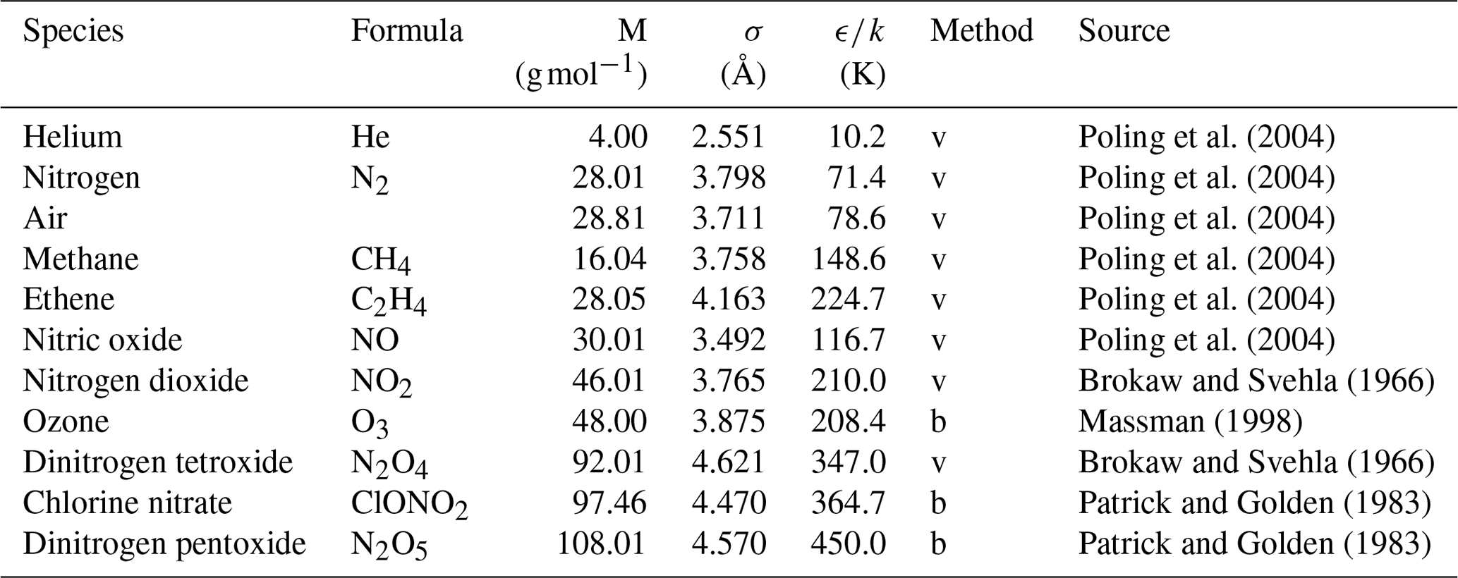
The letter v – obtained from viscosity data; b – obtained from Tb and Vb using Eq. (4).
Chapman and Enskog derived the following equation from the kinetic theory of gases for the molecular binary diffusion coefficient:
where m is the mass of the molecules, k is the Boltzmann constant, p is the pressure and T is the absolute temperature. σAB is the characteristic length of the intermolecular force law, and ΩD is the dimensionless collision integral of diffusion. It depends on the temperature and the characteristic energy ϵAB of the Lennard–Jones potential describing the intermolecular force (Poling et al., 2004; Marrero and Mason, 1972). ΩD as a function of temperature is expressed by the fit function
where , A=1.06036, B=0.15610, C=0.19300, D=0.47635, E=1.03587, F=1.52996, G=1.76474 and H=3.89411 (Neufeld et al., 1972; Poling et al., 2004). The equations
are usually employed to relate the interaction parameters of the Lennard–Jones potential between components A and B to the interaction potential parameters of the individual components. A tabulation of the potential parameters of the species considered in this work is given in Table 1. The Lennard–Jones parameters σ and ϵ are generally not available for unstable atmospheric trace gases. Patrick and Golden (1983) estimated them by using the equations
from Tb the normal boiling point temperature and Vb the molar volume at boiling point. In cases in which Vb cannot be determined experimentally, it is obtained from tables of atomic volumes using the LeBas method. Patrick and Golden (1983) assumed the systematic errors of σ and ϵ obtained by this method to be ≤20 %.
The diffusion coefficient as a function of pressure in a narrow temperature range close to the reference temperature T0 is usually expressed as
where T0=273.15 K is the standard temperature and p0=101 325 Pa is standard pressure (STP). Close to the reference temperature T0, the temperature coefficient b can be calculated as follows (Poling et al., 2004):
From Eq. (2) it is obtained by derivation
Fuller et al. (1966) developed a simple correlation equation for the estimation of gas-phase diffusion coefficients using additive atomic volumes VA and VB for each species. With the molar masses MA and MB ([M]= g mol−1) of each species and [p]= bar, the diffusion coefficient ([D]= cm2 s−1) is given by
Tabulations of atomic volume increments are summarized by Poling et al. (2004) and Tang et al. (2014a).
In the atmosphere, for typical submicron-sized aerosol particles, gas-phase diffusion does not usually limit uptake. Therefore, for modeling atmospheric processes, it is sufficient to use diffusion coefficients obtained using the Fuller method. However, in many laboratory experiments for the measurement of mass accommodation coefficients, conditions are such that gas-phase diffusion limitations need to be taken into account (Kirchner et al., 1990; Müller and Heal, 2002; Davidovits et al., 2006).
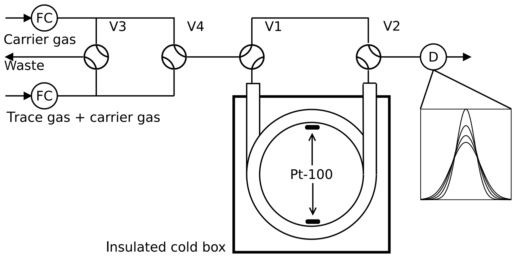
Figure 1Arrested flow method: a pulse of trace gas is introduced into the column by simultaneously switching valves V3 and V4 for a short time. After the peak has reached the middle of the column, the carrier gas is bypassed by switching V1 and V2 for arrest times ta between 0 and 200 s. After each arrest time ta the corresponding peak shape is recorded by the detector D. The gas flow is controlled by flow controller FC.
2.1 Arrested flow method
The arrested flow (AF) method was first described by Knox and McLaren (1964) and McCoy and Moffat (1986): the diffusion coefficient of a given trace gas is derived from the broadening of width ςt of trace gas plugs arrested for different times in a long void gas chromatography glass column (length l=2.8 m, radius r=0.189 cm). A plug is generated by injecting a small amount of dilute trace gas into a steady flow of carrier gas by means of computer-controlled solenoid valves. The flow is arrested when the plug has traveled halfway down the tube; see Fig. 1. In the absence of turbulence, the initial plug profile spreads out along the tube by molecular diffusion only. Until the flow is arrested, the box profile of the trace gas is reshaped to Gaussian by Taylor diffusion (Taylor, 1953, 1954) if the condition
is fulfilled, where is the carrier gas flow rate. After a given arrest time ta, the trace gas is eluted with ≈ 20 sccm (1 sccm = 1 mL min−1 at 273.15 K and 1013 hPa) and the concentration profile is measured with a suitable gas chromatography detector. This procedure is repeated for different arrest times ta. The experimental peak profiles are fitted to Gaussians to determine the peak variance . According to theory based on Fick's second law of diffusion,
a plot of versus arrest time ta should be linear. The slope of the plot of ςz vs. ta is given by
Since the variance is measured in units of time, it has to be converted to units of length using the gas flow speed v in the column
From the carrier gas mass flow , temperature T and pressure p in the column that approximately equals atmospheric pressure, the flow speed can be determined by
The column is embedded in an aluminum block cooled by a recirculating cryostat (Lauda RLS6). The aluminum block is mounted in a plastic box insulated by Styrodur. The column temperature homogeneity is monitored with two Pt-100 sensors connected to the upper and lower parts of the column coil. The solenoid valves are connected by 1∕16” Teflon tubes and controlled by a computer using the software Asyst 3.1 (Keithley). At each temperature, 12 to 20 peaks are recorded at different arrest times.
The systematic error of the determined diffusion coefficients using this method primarily depends on the systematic error of measuring the inner diameter of the column and the systematic error of the mass flow rate. A Teflon tube pushed through the column was used to determine the length of the column. The void volume of the column was determined by filling the column with water and measuring the weight of the water. From volume and length, the cross-sectional area and radius are calculated, yielding a mean radius with a systematic error of 0.5 %. After the experiments, the column was cut into small fragments. The inner diameter of these fragments was measured using a caliper gauge. We found that the inner diameter synchronously changes with column winding with a variability of 1 %. When using Eq. (14) to transform Δςt to Δςz, not the mean velocity but the actual velocity v and radius r at the location where the peak is arrested are relevant. Therefore, the actual systematic error of the radius is about 1 %. The mass flow controllers were calibrated using a soap bubble flow meter. Thus, the systematic error of the mass flow rate is about 1.5 %. This sums up to a total theoretical systematic error for the AF method of about 7 %. The random error of the method is about >0.4 %, twice the repeatability >0.2 % of the flow rate.
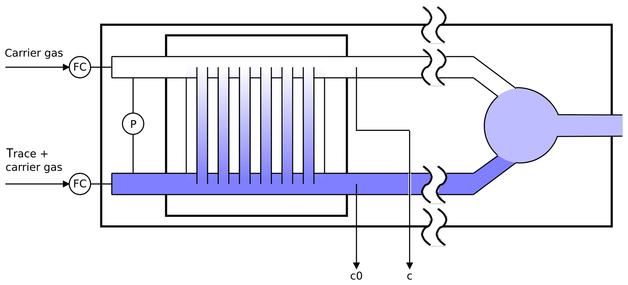
Figure 2Schematic diagram of the twin tube experiment (not to scale): a diffusion bridge connects two flow tubes. Downstream of the diffusion bridge some gas is continuously sampled for analysis to determine the trace gas concentrations c0 and c.
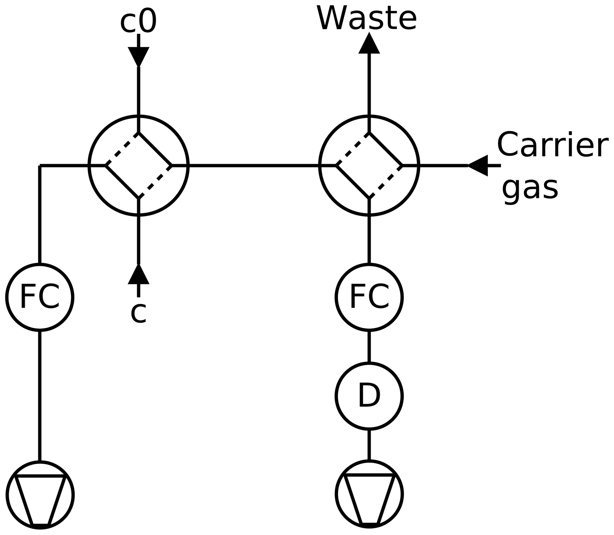
Figure 3Twin tube method, continuous mode: a partial current is sucked through the detector D by a mass flow controller FC. A second four-port valve enables switching the detector to pure carrier gas to record the baseline.
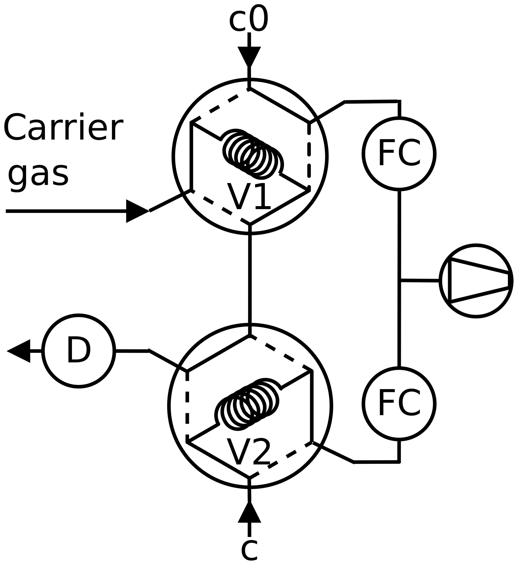
Figure 4Twin tube method, peak mode: the carrier gas is admitted first through the sample loop V1 or V2 of a six-port valve. Then the content of the sample loop is pushed into the detector as peak after switching the six-port valve.
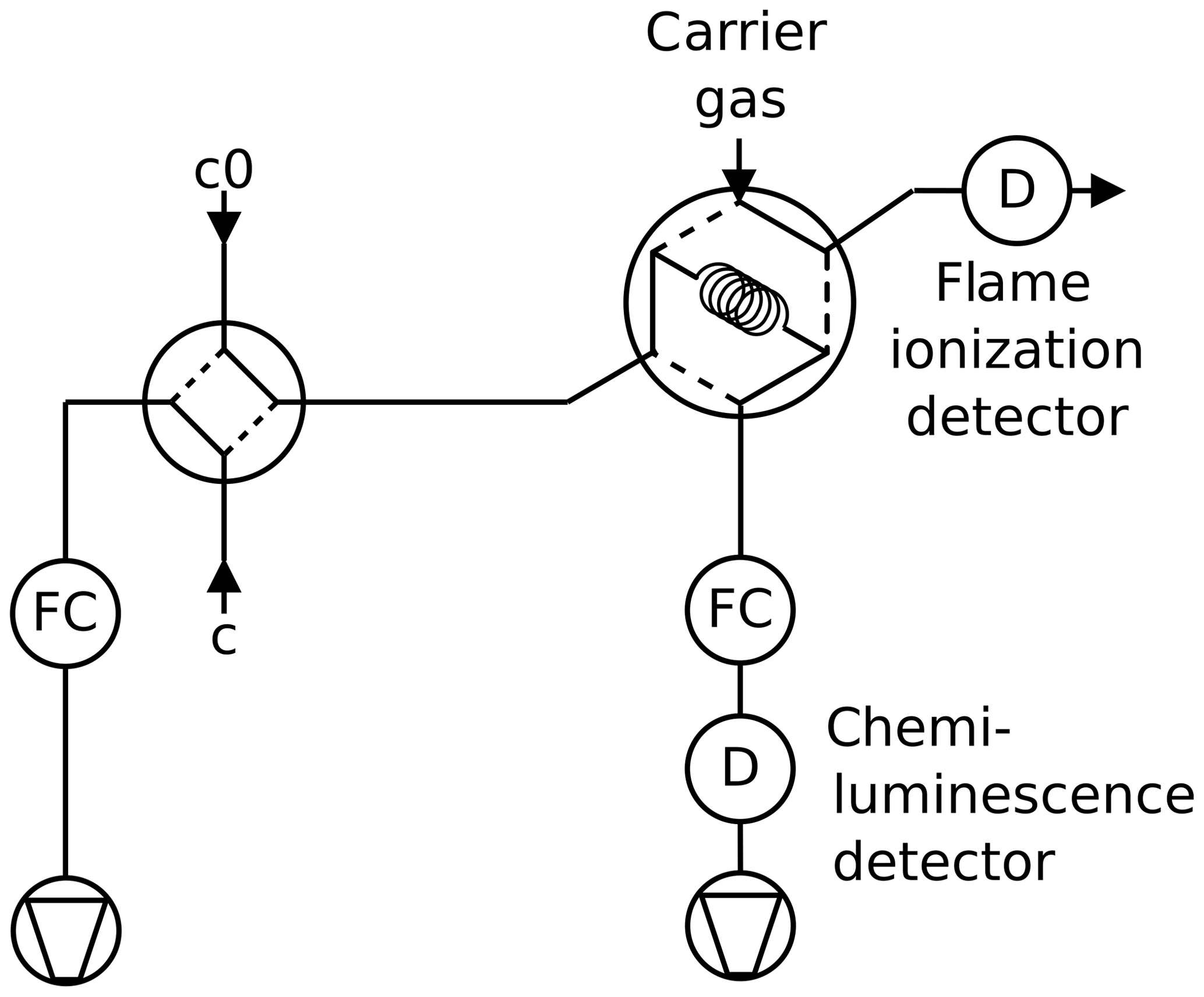
Figure 5Twin tube method with internal standard as used for NO2 in N2: the species under investigation is monitored in continuous mode, and the internal standard is sampled by a six-port valve and detected by a flame ionization detector.
2.2 Twin tube method
The twin tube (TT) method is a steady-state technique for diffusion coefficient measurements over a wide temperature range using a diffusion bridge (Marrero and Mason, 1972). It is insensitive to wall adsorption effects, which may invalidate AF measurements at low temperature. Our apparatus consists of two parallel horizontal flow tubes (length 2 m, inner diameter 10 mm) connected by a bunch of n=220 carefully thermostatted fused silica capillaries of radius and length ; see Fig. 2. The capillaries are embedded in a block made of brass. The cooling liquid of a cryostat (Lauda RLS6) circulates through the brass block, thereby covering the range from ambient temperature down to 198 K. Close to the diffusion bridge, the temperature in the block is measured with two Pt-100 sensors. The capillaries are pasted into two parallel slits in a short section of the parallel flow tubes that is made of stainless steel. Upstream and downstream of the brass block, the flow tubes consist of glass. The entire apparatus consisting of the flow tubes and the diffusion bridge is housed in a large insulated box that can be cooled down to 260 K. After changing the setting of the recirculating thermostat by an increment of 10 K it takes about 1 h until the temperature of the diffusion bridge has equilibrated.
Pure carrier gas is flown through one of the flow tubes, while a constant trace gas concentration c0 is maintained in the other. A concentration gradient is established along the capillaries. This gives rise to a constant flux JD by molecular diffusion through the diffusion bridge described by Fick's first law of diffusion:
where c is the trace gas concentration at the low concentration end. Pressure differences between the flow tubes are carefully eliminated to suppress trace gas transport by viscous flow through the capillaries. This requires that both flow tubes are totally symmetric. The difference pressure is monitored using a differential high-accuracy pressure transducer (MKS model 398, measuring range 10−4 to 1 Torr). By measuring the concentration ratio in both flow tubes, downstream of the diffusion bridge the diffusion coefficient is obtained by
when c≪c0, where is the volume flow rate of the carrier gas. The ratio of mass transport by viscous flow to diffusion flow through the capillaries is given by (viscosity η)
Therefore, the ratio of interfering viscous trace gas to mass flow by diffusion was minimized by using narrow capillaries. For the diffusion of NO2 in N2 at standard pressure and temperature, the fraction of viscous flow can be held <1 % when keeping the differential pressure Torr. During the TT experiments the differential pressure was maintained low so that the fraction of viscous flow was less than 0.3 %.
A trace gas detector is required that is linear over a wide concentration range and stable over time. Depending on the trace gas and the detector properties, the trace gas can either be detected by continuous mode (Fig. 3) or by peak mode (Fig. 4). The low concentration is determined with a random error of about 1 %. The signal of the trace gas detector is fed into an A/D converter with 16 bit resolution (Data Translation DT2705/5715A).
The supplier of the capillary columns used in this work as raw material for assembling the diffusion bridge reports the inner diameter with a systematic error of 10 %. This is too much for the measurement of diffusion coefficients. Therefore, two segments of the column were used to determine the inner diameter by weighing an empty and a water-filled section of the capillary column. Thereby, the radius of the diffusion bridge capillaries was determined with a systematic error of 1 %. We tried to validate the result with electron micrography of two cross sections of the column material. However, the systematic error of the inner diameter measured by electron micrography is about 5 %. When assuming a systematic error of the flow rate of 1.5 %, this results in a total systematic error of the method of <4 %. The random error of the method depends on the random error of about 1 % of the determination of the lower concentration c.
Later on during the experiments it was found that some capillaries of the diffusion bridge became blocked by dust or condensed matter. Fortunately, the TT method can be utilized to measure the diffusion coefficients of several species simultaneously when using the peak mode and a gas chromatograph as a detector. If the diffusion coefficient of one of the trace gases has been determined with another reliable technique at one temperature, this diffusion coefficient can be used as an internal standard; see Fig. 5. It is assumed that the effective area of the capillaries is independent of temperature.
To determine D0 and b, the diffusion coefficients obtained at different temperatures were fitted by nonlinear regression to Eq. (5). They were weighted by the inverse of their statistical error where available. The results are summarized in Table 3 together with the diffusion coefficients calculated by the Chapman–Enskog theory using Eq. (1) and the Fuller method using Eq. (10). The input parameters used are summarized in Table 1.
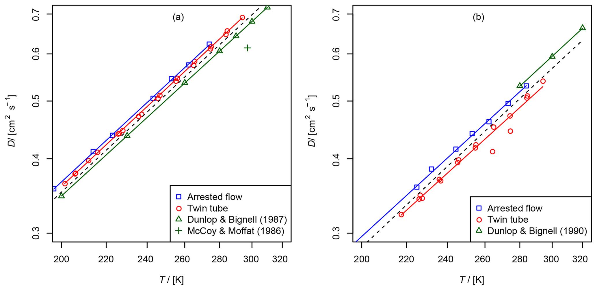
Figure 6Comparison of diffusion coefficients obtained by the AF and TT method: (a) diffusion coefficient of methane in helium compared to data from Dunlop and Bignell (1987) (fit , b=1.66) and at 297 K from McCoy and Moffat (1986). (b) Diffusion coefficient of ethene in helium compared to data from Dunlop and Bignell (1990) (fit , b=1.68). The dashed line is calculated by the Lennard–Jones model.
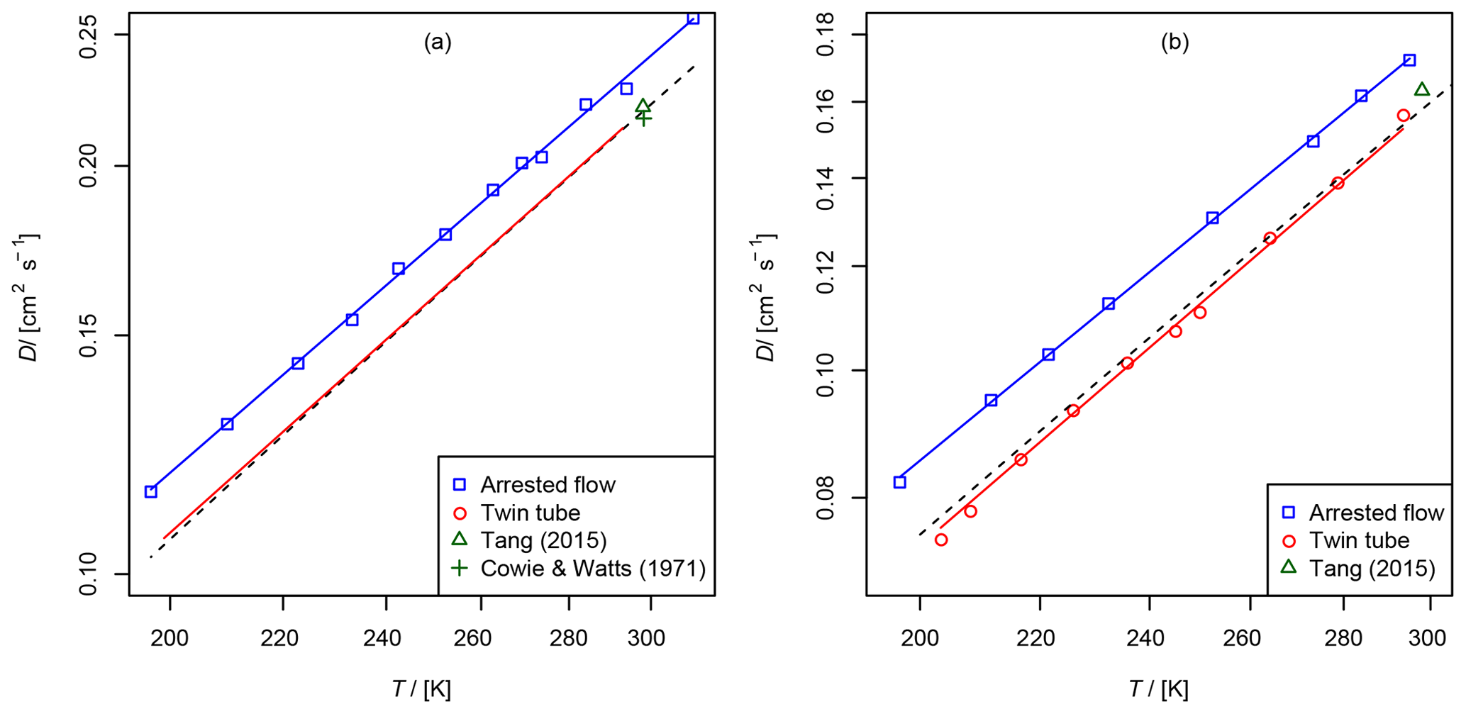
Figure 7(a) Diffusion coefficient of methane in air, recommended value of at 298 K from Tang et al. (2015) and from Cowie and Watts (1971) at 298.2 K. For the TT method only the fit function is shown. (b) Diffusion coefficient of ethene in air as a function of temperature, recommended value of Tang et al. (2015) at 298 K. The dashed line is calculated using the Lennard–Jones model.
3.1 Method validation
3.1.1 Diffusion of methane (CH4) and ethene (C2H4) in helium and air
These gases were investigated with both methods for validation purposes. They are stable and non-adsorbing, and there are reference data on the diffusion coefficients in the literature. The diffusion coefficients in helium have been measured previously over a wider temperature range with high precision and accuracy by Dunlop and Bignell (1987) for methane and Dunlop and Bignell (1990) for ethene. Evaluated diffusion coefficients of hydrocarbons in air at 298 K are reported in the review of Tang et al. (2015). In addition, the diffusion coefficients can be calculated using the Lennard–Jones model and the Chapman–Enskog theory using Eq. (1).
We used a flame ionization detector (Carlo Erba FID 40 with EL980 control unit), which is fast, sensitive and linear over a wide concentration range, to measure the hydrocarbons. For the AF experiments, 0.1 % methane or ethane in helium or air was injected as a 300 ms pulse. About 20–26 sccm was used as a flow rate. The arrest time was varied from 0 to 200 s. For the TT experiments 0.5 and 1 % methane in air, 0.4 % methane in He, 0.4 % ethene in He, and 0.5 % ethene in air were admitted into the flow tube. Downstream of the diffusion bridge, the trace gas was analyzed using the peak mode setup; see Fig. 4.
Table 2Measured diffusion coefficients D at the reference temperature T and standard pressure (101 325 Pa); reference data of diffusion coefficients Dr. With 298 K as a reference temperature, the measured diffusion coefficients were extrapolated to this temperature using Eq. (5).
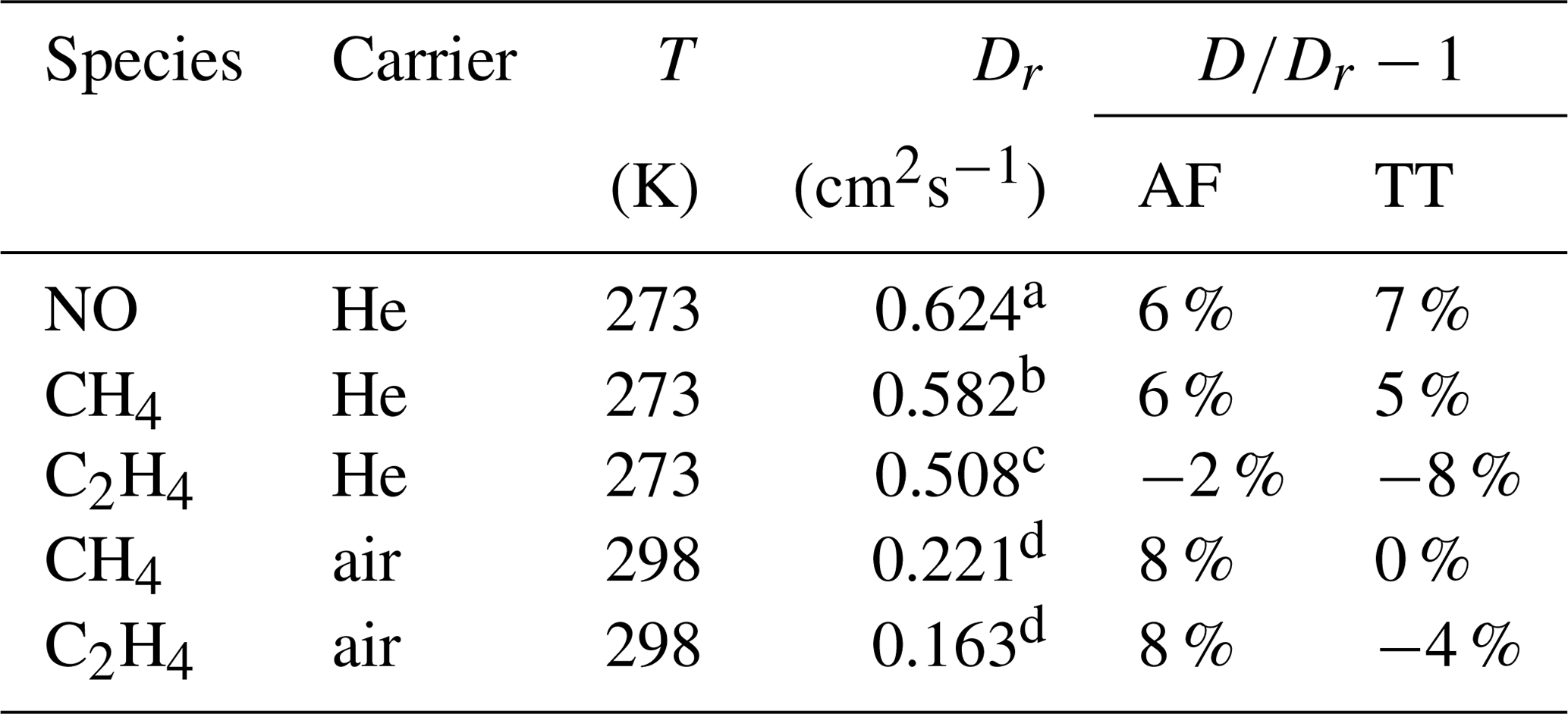
Source: a Dunlop and Bignell (1992), b Dunlop and Bignell (1987), c Dunlop and Bignell (1990), d Tang et al. (2015).
The results are summarized in Tables 2 and 3 as well as in Figs. 6 and 7. Higher diffusion coefficients were found for the AF method compared to the TT method.
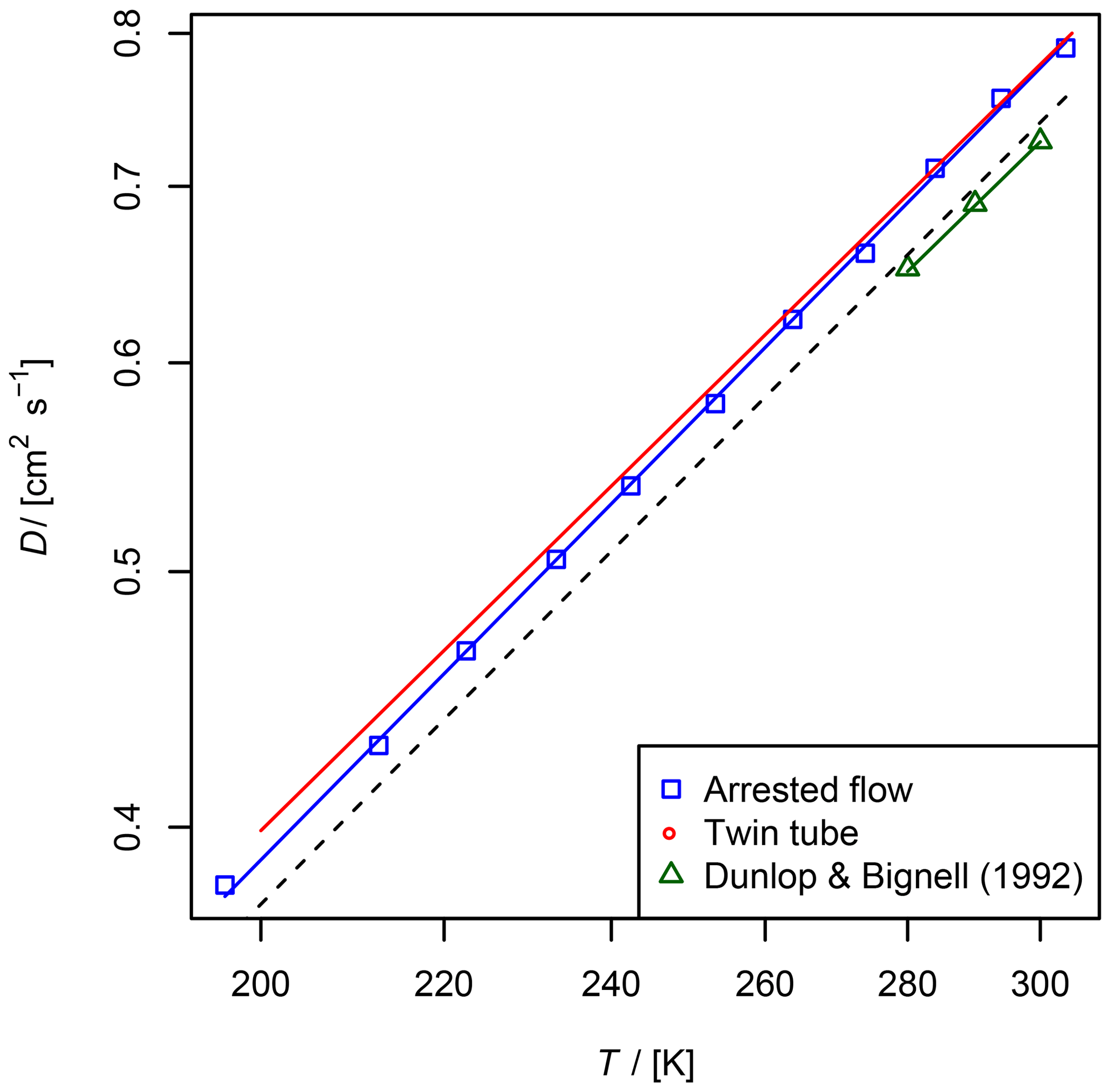
Figure 8Diffusion coefficient of NO in He measured by the AF and TT method as a function of temperature. For the TT method only the fit function is shown. Experimental results from Dunlop and Bignell (1992) and a fit to Eq. (5) with D0=0.624 and b=1.64 are displayed as a reference. The dashed line is calculated using the Lennard–Jones model.
3.1.2 Diffusion of nitric oxide (NO) in helium
NO was monitored by a chemiluminescence detector (Marić et al., 1989), which was adapted to the lower flow rates of the diffusion experiments. In the detector, NO reacts with O3 in a low-pressure reaction chamber (0.9–2 mbar) in a chemiluminescence reaction:
The emitted photons were detected using a Hamamatsu R562 photomultiplier tube.
For the AF experiment 100 ppm NO was injected as a 300 ms pulse into the flow tube with a flow rate of 22.5 sccm. The valves were connected using stainless-steel tubes. For the TT experiment 30–70 ppm NO in He was admitted into the diffusion bridge. The setup displayed in Fig. 3 was used to monitor NO in the continuous mode. It was found that after measuring the high-concentration c0, several hours are needed until the baseline has stabilized when measuring a clean carrier gas. Therefore, it is not possible to measure c and c0 in succession. Thus, first c0 was measured at room temperature. Then the detector was switched to clean carrier gas until the baseline stabilized. Then c was measured after lowering the temperature until the signal stabilized. After arriving at 200 K, c0 was measured again. Then the measurement was repeated by raising the temperature stepwise. Therefore, the complete measurement extended over several days.
The diffusion coefficients for NO obtained by the two methods are in fair agreement with the reference data from Dunlop and Bignell (1992); see Fig. 8 and Table 2. In contrast to the diffusion coefficients of methane and ethane, the diffusion coefficients obtained by the TT method are slightly larger than the diffusion coefficients obtained by the AF method.
Comparing all diffusion coefficients obtained for stable gases to reference data, it is found that the deviation of the AF and TT method is less than 8 % compared to the reference data. However, for the TT method this is a little more, as expected because of theoretical systematic error, which can be explained by decreasing effective areas of the diffusion capillaries.
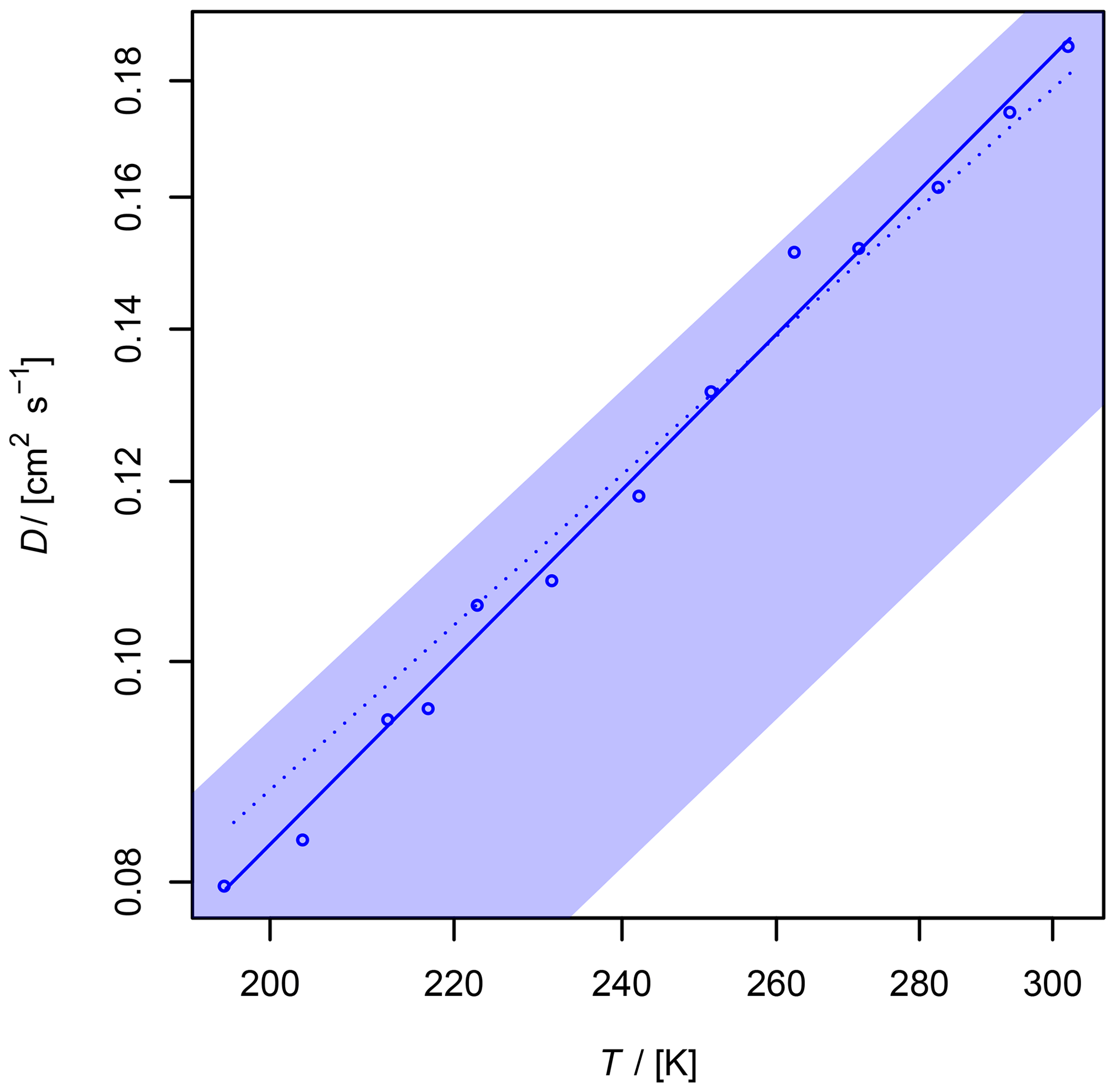
Figure 9Diffusion coefficient of O3 in air as a function of temperature. The shaded area shows the diffusion coefficient expected by the Lennard–Jones model. The upper border is calculated with and the lower border with using Eq. (1), corresponding to a 20 % uncertainty of σAB and ϵAB. The dotted line is calculated by Fuller's model.
3.2 Diffusion of atmospheric trace gases
3.2.1 Diffusion of ozone (O3) in air
The diffusion coefficient of ozone in air has never been measured before. Ivanov et al. (2007) reported cm2 s−1 for the diffusion of O3 in He at 298 K. Since ozone is an unstable but non-adsorbing species, only the AF method was used for the determination of the diffusion coefficient. A fast and sensitive ozone detector is required to record the ozone peaks leaving the column. A suitable detection technique is chemiluminescence arising from the reaction of ozone with coumarin 47 (Lambda Physik; 7-diethylamino-4-methylcoumarin) adsorbed on silica-gel plates (Schurath et al., 1991). Chemiluminescence is emitted in the range λ= 440–550 nm, which is detected by a photomultiplier (Hamamatsu 931 B). The anode current was admitted through a 100 kΩ resistor and measured as voltage by a microvoltmeter (Keithley model 155).
Ozone-containing air was generated in an aluminum block enclosing an elliptically shaped polished chamber. A rod-shaped low-pressure Hg UV lamp and a quartz tube with air running through are mounted parallel in the focal lines of the elliptically shaped chamber. Thereby, the UV radiation is focused to the air flowing through the quartz tube (Becker et al., 1975). Five blocks arranged in series were used, yielding an ozone concentration of about 40 ppm.
The injection time was varied from 250 to 500 ms, and the arrest time was varied from 0 to 360 s. It was found that the maxima of the eluted peaks did not coincide: peaks arrested longer were eluted later. Later it was found that this was caused by leaking neoprene seals on the solenoid valves. Therefore, at some temperatures only arrest times of less than 100 s were included in the fit of vs. ta. The statistical error of the slope of vs. ta was up to 3.7 %.
With regard to the systematic error of 7 % in the AF method for the diffusion coefficients (Section 3.1.1), the obtained value with error ranges is cm2 s−1. This value is in accordance with the value of D0=0.1444 cm2 s−1 estimated by Massman (1998) from critical constants using the model of Chen and Othmer (1962).
Fuller et al. (1966)Table 3Diffusion coefficient D0 at standard temperature (273.15 K) and pressure (101 325 Pa) and temperature coefficient b as results from the fit of Eq. (5) to the measured data. The errors listed are the errors obtained by the fit. Diffusion coefficients calculated by the Lennard–Jones and Fuller method are displayed for comparison. D0(N2O4) is estimated by the nonlinear regression of Eq. (23), arbitrarily setting b=1.75. For N2O5 the fit parameters of Eq. (15) are displayed.
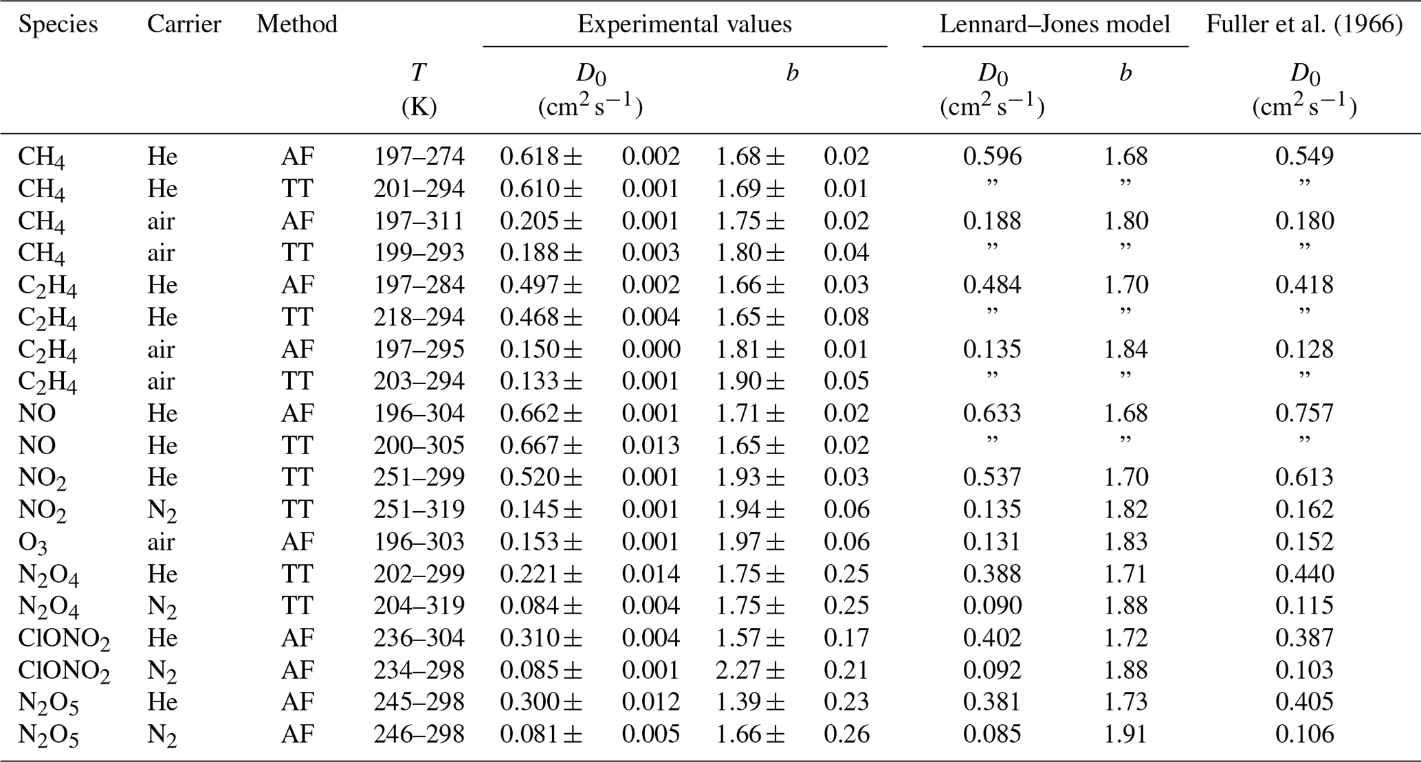
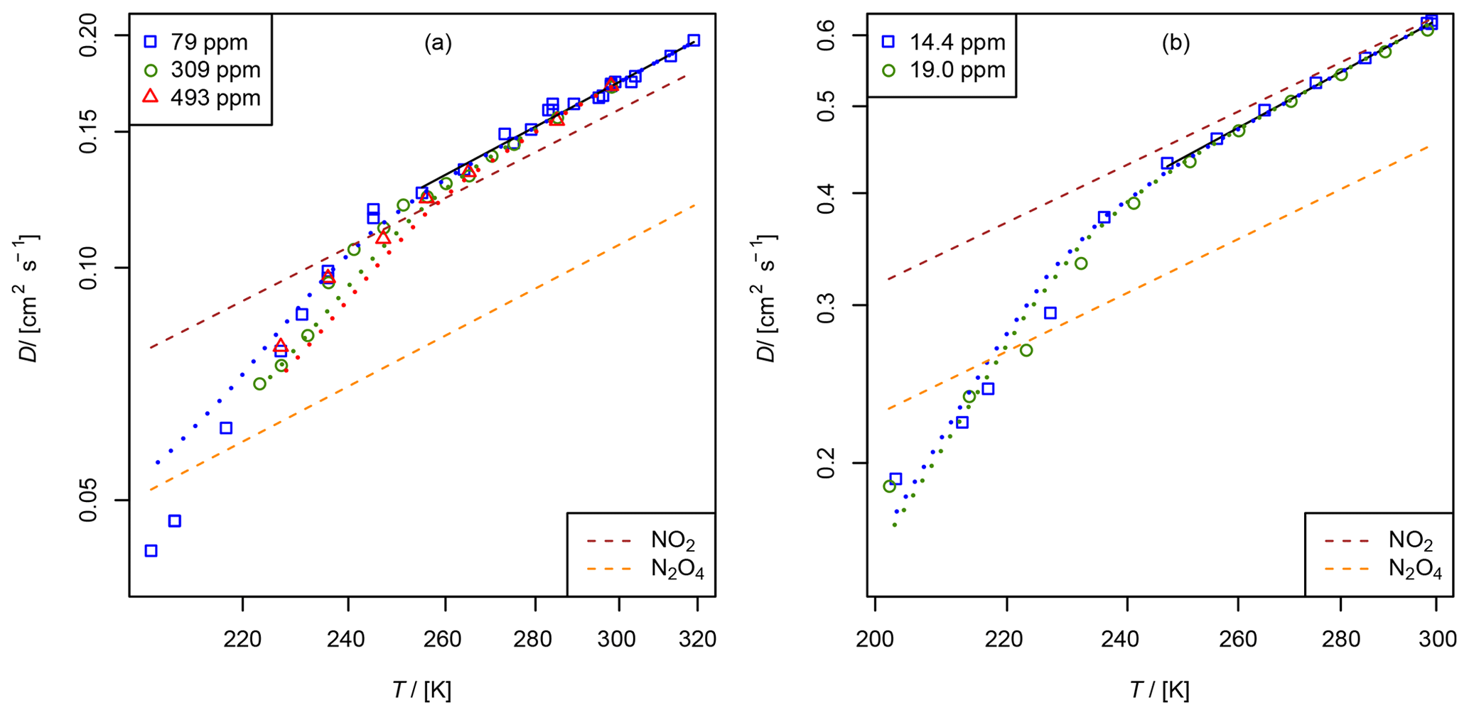
Figure 10Apparent diffusion coefficient D(NIV) of NO2∕N2O4 in N2 (a) and He (b) as a function of temperature. Black solid line: fit of Eq. (5) to data points with α>0.95. The dashed lines are calculated using the Lennard–Jones model. The dotted curves are fit curves of Eq. (23) by setting b(N2O4)=1.75.
3.2.2 Diffusion of nitrogen dioxide (NO2) and dinitrogen tetroxide (N2O4) in helium and nitrogen
NO2 is in equilibrium with its dimer,
Therefore, a pure sample of NO2 for determinations of D is not available. Chambers and Sherwood (1937) assumed that the ratio of , yielding in nitrogen from their value of cm2 s−1. Massman (1998) estimated D0(NO2)= 0.146 cm2 s−1 from in nitrogen reported by Sviridenko et al. (1973). Since NO2 is an adsorbing species, the diffusion coefficient can only be measured using the TT method. The total flux of the pseudo-species NIV = NO2 + 2 N2O4 through the capillaries is given by
At higher temperatures and when keeping the concentration of NO2 low, the diffusion of N2O4 can be neglected. The degree of dissociation,
can be calculated from the equilibrium constant
where bar. The equilibrium constant close to 250 K is estimated from JANAF Thermochemical Tables (NIST, 1998):
Actually, D(NIV) is determined using the TT experiment, depending on D(NO2) and D(N2O4) (see Supplement S1):
A thermostatted permeation tube consisting of a PTFE tube (2.5 cm length, 4.3 mm diameter) closed with two Swagelok connectors filled with liquid N2O4 is used as an NO2 source. The measurements were performed in the temperature range from 200 to 300 K. NO2 was measured as NO using the chemiluminescence analyzer preceded by a thermal converter. The converter, which consisted of a gold wire in a thin quartz tube heated to 540 K, was run with 1.5–3 % methanol vapor instead of the more commonly used CO reagent (Langenberg et al., 1998). This eliminated poisoning of the gold wire, which occurs when metal carbonyl impurities are present in the CO gas. The total conversion rate is unknown. However, for the TT experiment, it is only required that the conversion rate is independent of concentration, which was checked for the concentration range of 3 to 100 ppm NO2 by a dynamic dilution experiment. NO2 was monitored using the continuous mode in Fig. 5. In order to compensate for aging effects of the capillary bridge, CH4 was admixed as an internal standard to the carrier gas flowing through the NO2 permeation source. The four-port valve in front of the detector was replaced by a six-port valve (Valco UC10W, 125 µm sample loop), which enables the detection of CH4 by the flame ionization detector. For CH4 in He cm2 s−1 at 273.15 K (Dunlop and Bignell, 1987) and for CH4 in N2 cm2 s−1 at 298 K (Mueller and Cahill, 1964) were chosen as reference diffusion coefficients for the internal standard. The measurement was performed in a similar manner as the NO measurement with the TT experiment by lowering and raising the temperature stepwise. Above 250 K the statistical error of the low concentration is about 3 %. However, below 250 K signal stability was low. In contrast to the measurements above 250 K, apparent D(NIV) measured at a certain temperature by lowering the temperature stepwise does not reproduce the value of D(NIV) measured by raising the temperature stepwise.
Figure 10 displays the obtained diffusion coefficients of the pseudo-species NIV as a function of temperature. It is obvious that below 250 K the plot deviates. Above 250 K diffusion of N2O4 can be neglected because N2O4 is mostly dissociated in the concentration range of our study. To estimate the diffusion coefficient of NO2 only data points with a dissociation degree α>0.95 were included in the fit of Eq. (5). Thus, regarding the errors of the diffusion coefficients of the internal standards, the diffusion coefficients for NO2 at STP are cm2 s−1 and cm2 s−1 in helium and nitrogen, respectively.
To determine D0(N2O4), Eq. (23) was fitted to experimental data on D(NIV) vs. T and p(NIV) by nonlinear regression. The temperature dependency of D(NIV) was described by Eq. (5) and α as a function of temperature, and p(NIV) was calculated using Eq. (21). D0(NO2) and b(NO2) were taken as fixed input parameters from the fit of Eq. (5) as described above. However, an independent determination of D0(N2O4) and b(N2O4) was not possible. Therefore, b(N2O4)=1.75 was set arbitrarily, yielding the diffusion coefficients listed in Table 3. Since b(N2O4) is expected in the range 1.5 to 2, the fit was repeated setting b=2 and b(N2O4)=1.5 to estimate the upper and lower limit of D0(N2O4) listed in Table 3. Compared to the diffusion coefficient of N2O4 in N2, the diffusion coefficient in He determined by the fit is much lower than the diffusion coefficient calculated by the Lennard–Jones model. In addition, our values are lower than the values of Sviridenko et al. (1973). We therefore consider our diffusion coefficients for N2O4 to be unreliable. However, we can explain the observed temperature dependency of D(NIV) in the transition to lower temperatures.
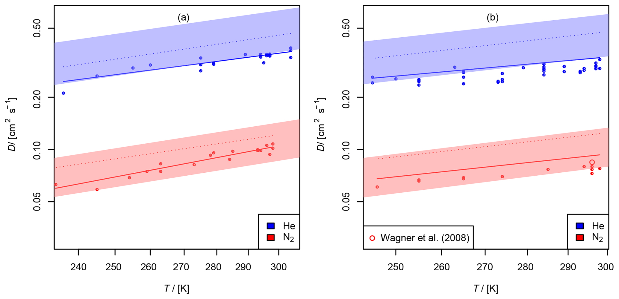
Figure 11(a) Diffusion coefficient of chlorine nitrate in helium and nitrogen; (b) diffusion coefficient of dinitrogen pentoxide in helium and nitrogen as a function of temperature. The experimental result of 0.085 cm2 s−1 from Wagner et al. (2008) is displayed for comparison. The shaded areas show the diffusion coefficients expected by the Lennard–Jones model. The dotted lines are calculated by Fuller's model. The solid lines displayed for N2O5 are calculated using Eq. (15) extrapolating to .
3.2.3 Diffusion of chlorine nitrate (ClONO2) in helium and nitrogen
Chlorine nitrate is an unstable compound. Therefore, the diffusion coefficient can only be measured using the AF method and not by the TT method. Chlorine nitrate was prepared by the reaction (Davidson et al., 1987)
Cl2O was prepared by admitting chlorine into a column filled with Raschig rings covered with freshly precipitated HgO (Schmeisser et al., 1967):
The formed Cl2O was condensed over N2O5 in a cold trap cooled with liquid nitrogen. Then the cold trap was cooled with ethanol at 193 K, which was allowed to warm up to 253 K within about 15 h.
The identity of the product was checked by an FTIR spectrometer (Nicolet, model Protégé 460) with a 10 m absorption path. The spectrum was recorded with 1 cm−1 resolution. ClONO2 was characterized by typical bands at 535–580, 750–825, 1270–1320 and 1695–1770 cm−1 compared to reference spectra measured by Davidson et al. (1987) and Orphal et al. (1997). No contamination of N2O5, NO2 and HCl was found.
Chlorine nitrate dissociates by the equilibrium reaction
The half-life of chlorine nitrate with respect to the thermal decomposition is 11 min at 300 K and about 7.8 h at 273 K. In addition to homogeneous dissociation, chlorine nitrate is lost by heterogeneous reaction with adsorbed water on the column surface (Tang et al., 2016):
To minimize this interference, the column was preconditioned with chlorine nitrate to remove moisture. During the first series of measurements with He as a carrier gas, chlorine nitrate was continuously admitted into the column for 10–15 min prior to the experiments. However, due to desorption the baseline stabilized only after some time. Therefore, during the second series of measurements with N2 as a carrier gas, series of peaks of chlorine nitrate were admitted into the column until the peak size stabilized. During one series of measurements, 16 peaks covering arrest times from 0 to 100 s and carrier gas flow rates of 19.6 sccm N2 and 28.6 sccm He were measured. The diffusion coefficient was measured in a temperature range of 235 to 300 K.
The detection of chlorine nitrate was performed as described by Anderson and Fahey (1990): an excess of NO (30–75 ppm) was added as a constant flow of 6.5–8 sccm in N2 before the detector by a T-tube. Behind the T-tube a glass capillary of 8 cm length and 0.1 cm inner diameter was mounted. The capillary was inserted in a stainless-steel tube, which was heated on a length of 1.7 cm to 433 K by two heating resistors. In the heating zone, chlorine nitrate is dissociated to ClO by Reaction R5. By subsequent scavenging reactions, NO is irreversibly removed.
A complete conversion of chlorine nitrate with NO is assumed. The drop in NO concentration equals the ClONO2 concentration and was monitored using the chemiluminescence detector.
It is presumed that the chlorine nitrate loss processes during peak arrest is a pure first-order process, which is a requirement for the application of the AF method. To check the first-order kinetics, logarithmic peak areas as a measure for the chlorine nitrate concentration were plotted against the arrest time, yielding a straight line. This validated the first-order characteristic of the chlorine loss process. The first-order loss constants ranged from to s−1. During the experiments with N2 as a carrier gas, loss rates increased with decreasing temperature. During the experiments with He, loss rates increased with increasing temperature. However, for the He experiments, a less effective preconditioning technique was applied, as described above.
The diffusion coefficients obtained at different temperatures are displayed in Fig. 11 (a). When taking a systematic error of 7 % for the AF method into account, the diffusion coefficients at STP are and cm2 s−1 in helium and nitrogen, respectively.
3.2.4 Diffusion of dinitrogen pentoxide (N2O5) in helium and nitrogen
Crystalline N2O5 was synthesized as described by Davidson et al. (1978) and Tang et al. (2014b): a small flow of pure NO is mixed with O3∕O2 in a glass reactor, trapping the product at 193 K using a cold trap immersed in a cold ethanol bath. O3 was generated in pure dry O2 with a silent discharge ozone generator (Sorbios, model GSG). After mixing NO with O3∕O2 in the glass reactor, a brown color appeared initially, indicating the formation of NO2:
After about 3 h, the addition of NO is stopped and the cooling bath of the cold trap is removed. To remove traces of NO2, the product is transferred into a second cold trap using an O3∕O2 stream. By means of a cryostat, the synthesized N2O5 crystals were stored in an ethanol bath kept at 193 K. The identity of the product was checked by infrared spectroscopy. The spectrum was recorded with 1 cm−1 resolution. N2O5 was characterized by typical bands at 750, 860, 1250, 1340 and 1725 cm−1 reported by a reference spectrum measured by Cantrell et al. (1988).
The cold trap filled with N2O5 crystals was immersed in the bath of a cryostat (Lauda RLS 6) thermostatted at 235 to 250 K. Dried carrier gas was admitted through the cold trap. An upper limit of the partial pressure of N2O5 in contact with the solid can be estimated with data from McDaniel et al. (1988). This results in an upper limit of the mole fraction of about 0.1 to 0.6 %. The trace gas was admitted into the AF experiments using short Teflon tubes.
N2O5 was detected as already described by Fahey et al. (1985): N2O5 is thermally decomposed to NO2 and NO3 radicals, which are then titrated by NO to form NO2:
The drop in NO concentration is equal to the N2O5 concentration. NO was measured again by the chemiluminescence detector. Downstream of the AF experiment, a constant flow of 6–8 sccm of 30–45 ppm NO was added.
The diffusion coefficient of N2O5 was measured in the temperature range 245 to 298 K. Below 245 K no measurement was possible because N2O5 was totally adsorbed in the column. At one fixed temperature 16 peaks were measured using arrest times between 0 and 100 s. At the beginning of a measurement series, the column was preconditioned with carrier gas containing N2O5 to remove moisture for 15–20 min. Prior to a measurement with arrest time, a peak without arrest time was pushed trough the column. During one series of measurements 16 peaks covering arrest times from 0 to 100 s and carrier gas flow rates of 19.3 sccm N2 and 28.8 sccm He were measured.
Equation (5) was used to obtain cm2 s−1, in He, and cm2 s−1 and in N2. Thus, the observed temperature coefficient is much lower than expected from Chapman–Enskog theory. As long as the N2O5 loss process is purely first order, the peak variance should not be affected by loss processes. To check this, peak areas were determined by integration. Plots of log (peak area) versus arrest times yielded apparent first-order loss constants k1 ranging from to s−1. To check if D depends on k1, the diffusion coefficient was expressed by
as a function of T and k1. It was found that D not only significantly depends on T, but also on k1. With P, the probability of the null hypothesis, ) s (P<0.05) and s (P<0.06) were found for He and N2, respectively. One reason for this may be that the order of the loss process of N2O5 is less than first order. The other fit parameters are displayed in Table 3. For He as a carrier gas, a temperature coefficient of b<1.5 was found. Due to the small temperature range investigated, the temperature coefficient is rather uncertain. As a final result, for He and for N2 cm2 s−1 are obtained when considering the systematic error of 7 % for the AF method and the possible influence of dinitrogen pentoxide degradation on the diffusion coefficients obtained. Wagner et al. (2008) reported a diffusion coefficient of 0.085 cm2 s−1 for N2O5 in N2 at 760 Torr and 296 K, which is within the error limits of our result.
The AF method is best suited for the measurement of the diffusion coefficients of volatile non-adsorbing trace gases, even if the trace gas is unstable like ozone. However, it is required that the trace gas loss process is first order. Otherwise, the Gaussian peak shape is distorted and the variance of the peaks depends on species reactions. The TT method is best suited for stable but adsorbing species.
For stable nonpolar gases, diffusion coefficients can be estimated from viscosity data using the Lennard–Jones model with a systematic error of <5 %, which is smaller than the systematic errors of less than 7 % of the AF and TT methods. For unstable atmospherically relevant trace gases and polar gases, the Lennard–Jones model parameters cannot be obtained by viscosity measurements. They can only be estimated from critical temperatures and volumes. Where dipole–induced-dipole interactions come into play the systematic errors of the diffusion coefficients obtained in this way are of the same order as the errors of the diffusion coefficients of the unstable and reactive trace gases investigated in this study.
For the species investigated in this study, it is found that Fuller's method overestimates the diffusion coefficients of inorganic compounds with a systematic error of typically less than 35 % and underestimates the diffusion coefficients of organic compounds with a systematic error of less than 15 %.
Raw data on temperature-dependent diffusion coefficients are included in the Supplement. The sample code for the calculation of diffusion coefficients using the Lennard–Jones and the Fuller model written in the language R (R Core Team, 2017) is also included.
The supplement related to this article is available online at: https://doi.org/10.5194/acp-20-3669-2020-supplement.
Conceptualization and methodology were undertaken by SS, investigation was done by TC, DH and SS, formal analysis and visualization were performed by TC, DH, SL and SS, SL wrote the draft, and supervision and funding acquisition were carried out by US. All the authors have read and approved the final paper.
The authors declare that they have no conflict of interest.
Torsten Carstens acknowledges a doctoral grant from the Karlsruher Institut für Technologie. We thank Ralf Rubröder and Birgit Walter for setting up the AF experiment; Pete Boecker for the assistance measuring FT-IR spectra; Harald Saathoff for providing infrared spectra of N2O5, HCl and NO2; Ewald Hild for the preparation of electron micrographs of the fused silica columns; and Dieter Gauer for technical assistance.
This research has been supported by the Deutsche Forschungsgemeinschaft (grant nos. 457/8-1, 457/8-2, and 457/8-3) within the priority program “Basics of the Impact of Air and Space Transportation on the Atmosphere”.
This paper was edited by Daniel Knopf and reviewed by two anonymous referees.
Anderson, L. C. and Fahey, D. W.: Studies with nitryl hypochlorite: thermal dissociation rate and catalytic conversion to nitric oxide using an NO/O3 chemiluminescence detector, J. Phys. Chem., 94, 644–652, https://doi.org/10.1021/j100365a027, 1990. a
Becker, K., Heindrichs, A., and Schurath, U.: Ein transportables Gerät zur Kalibrierung von Ozonanalysatoren durch Messung der optischen Absorption, Staub Reinhalt. Luft, 35, 326–329, 1975. a
Brokaw, R. S. and Svehla, R. A.: Viscosity and Thermal Conductivity of the N2O4 ⇌ 2 NO2 System, J. Chem. Phys., 44, 4643–4645, https://doi.org/10.1063/1.1726692, 1966. a, b
Cantrell, C. A., Davidson, J. A., McDaniel, A. H., Shetter, R. E., and Calvert, J. G.: Infrared absorption cross sections for N2O5, Chem. Phys. Lett., 148, 358–363, https://doi.org/10.1016/0009-2614(88)87288-9, 1988. a
Chambers, F. S. and Sherwood, T. K.: Absorption of Nitrogen Dioxide by Aqueous Solutions, Ind. Eng. Chem., 29, 1415–1422, https://doi.org/10.1021/ie50336a022, 1937. a
Chen, N. and Othmer, D.: New generalized equation for gas diffusion coefficient, J. Chem. Eng. Data, 7, 37–41, https://doi.org/10.1021/je60012a011, 1962. a
Cowie, M. and Watts, H.: Diffusion of Methane and Chloromethanes in Air, Can. J. Chem., 49, 74–77, https://doi.org/10.1139/v71-011, 1971. a
Davidovits, P., Kolb, C. E., Williams, L. R., Jayne, J. T., and Worsnop, D. R.: Mass Accommodation and Chemical Reactions at Gas–Liquid Interfaces, Chem. Rev., 106, 1323–1354, https://doi.org/10.1021/cr040366k, pMID: 16608183, 2006. a
Davidson, J., Cantrell, C., Shetter, R., McDaniel, A., and Calvert, J.: Absolute Infrared Absorption Cross Sections for ClONO2 at 296 and 223 K, J. Geophys. Res., 92, 10921–10925, https://doi.org/10.1029/JD092iD09p10921, 1987. a, b
Davidson, J. A., Viggiano, A. A., Howard, C. J., Dotan, I., Fehsenfeld, F. C., Albritton, D. L., and Ferguson, E. E.: Rate constants for the reactions of , , NO+, H3O+, , , and halide ions with N2O5 at 300 K, J. Chem. Phys., 68, 2085–2087, https://doi.org/10.1063/1.436032, 1978. a
Dunlop, P. J. and Bignell, C.: Diffusion and thermal diffusion in binary mixtures of methane with noble gases and of argon with krypton, Physica A, 145, 584–596, https://doi.org/10.1016/0378-4371(87)90009-4, 1987. a, b, c, d
Dunlop, P. J. and Bignell, C. M.: The temperature and concentration dependencies of diffusion coefficients of some helium–hydrocarbon and helium–fluorocarbon systems, J. Chem. Phys., 93, 2701–2703, https://doi.org/10.1063/1.458908, 1990. a, b, c
Dunlop, P. J. and Bignell, C. M.: The Temperature and Concentration Dependences of Diffusion Coefficients of the Systems Ne–O2, Kr–O2, Xe–O2 and He–NO, Ber. Bunsen. Phys. Chem., 96, 1847–1848, https://doi.org/10.1002/bbpc.19920961211, 1992. a, b, c
Eller, A. S. D. and Sparks, J. P.: Predicting leaf-level fluxes of O3 and NO2: the relative roles of diffusion and biochemical processes, Plant Cell Environ., 29, 1742–1750, https://doi.org/10.1111/j.1365-3040.2006.01546.x, 2006. a
Fahey, D., Eubank, C., Hübler, G., and Fehsenfeld, F.: A calibrated source of N2O5, Atmos. Environ. (1967), 19, 1883–1890, https://doi.org/10.1016/0004-6981(85)90013-7, 1985. a
Fall, R. and Monson, R. K.: Isoprene Emission Rate and Intercellular Isoprene Concentration as Influenced by Stomatal Distribution and Conductance, Plant Physiol., 100, 987–992, https://doi.org/10.1104/pp.100.2.987, 1992. a
Fuller, E. N., Schettler, P. D., and Giddings, J. C.: New Method for Prediction of Binary Gas-phase Diffusion Coefficients, Ind. Eng. Chem., 58, 18–27, https://doi.org/10.1021/ie50677a007, 1966. a, b
Gu, W., Cheng, P., and Tang, M.: Compilation and evaluation of gas phase diffusion coefficients of halogenated organic compounds, Roy. Soc. Open Sci., 5, 171936, https://doi.org/10.1098/rsos.171936, 2018. a
Ivanov, A. V., Trakhtenberg, S., Bertram, A. K., Gershenzon, Y. M., and Molina, M. J.: OH, HO2, and Ozone Gaseous Diffusion Coefficients, J. Phys. Chem. A, 111, 1632–1637, https://doi.org/10.1021/jp066558w, pMID: 17298040, 2007. a
Kirchner, W., Welter, F., Bongartz, A., Kames, J., Schweighoefer, S., and Schurath, U.: Trace gas exchange at the air/water interface: Measurements of mass accommodation coefficients, J. Atmos. Chem., 10, 427–449, https://doi.org/10.1007/BF00115784, 1990. a
Knox, J. H. and McLaren, L.: A New Gas Chromatographic Method for Measuring Gaseous Diffusion Coefficients and Obstructive Factors, Anal. Chem., 36, 1477–1482, https://doi.org/10.1021/ac60214a017, 1964. a
Kolb, C. E., Cox, R. A., Abbatt, J. P. D., Ammann, M., Davis, E. J., Donaldson, D. J., Garrett, B. C., George, C., Griffiths, P. T., Hanson, D. R., Kulmala, M., McFiggans, G., Pöschl, U., Riipinen, I., Rossi, M. J., Rudich, Y., Wagner, P. E., Winkler, P. M., Worsnop, D. R., and O' Dowd, C. D.: An overview of current issues in the uptake of atmospheric trace gases by aerosols and clouds, Atmos. Chem. Phys., 10, 10561–10605, https://doi.org/10.5194/acp-10-10561-2010, 2010. a
Laisk, A., Kull, O., and Moldau, H.: Ozone Concentration in Leaf Intercellular Air Spaces Is Close to Zero, Plant Physiol., 90, 1163–1167, https://doi.org/10.1104/pp.90.3.1163, 1989. a
Langenberg, S., Proksch, V., and Schurath, U.: Solubilities and Diffusion of trace gases in cold sulfuric acid films, Atmos. Environ., 32, 3129–3137, https://doi.org/10.1016/S1352-2310(97)00490-1, 1998. a
Marić, D., Hans, W., and Schurath, U.: Measurements of N2O photolysis coefficients in the stratosphere: Comparison with model calculations, J. Atmos. Chem., 8, 19–40, https://doi.org/10.1007/BF00053814, 1989. a
Marrero, T. R. and Mason, E. A.: Gaseous Diffusion Coefficients, J. Phys. Chem. Ref. Data, 1, 3–118, https://doi.org/10.1063/1.3253094, 1972. a, b, c
Massman, W.: A review of the molecular diffusivities of H2O, CO2, CH4, CO, O3, SO2, NH3, N2O, NO, and NO2 in air, O2 and N2 near STP, Atmos. Environ., 32, 1111–1127, https://doi.org/10.1016/S1352-2310(97)00391-9, 1998. a, b, c, d
McCoy, B. J. and Moffat, A. J.: Arrested-flow Chromatographic Measurement of Gaseous Diffusion Coefficients, Chem. Eng. Commun., 47, 219–224, https://doi.org/10.1080/00986448608911765, 1986. a, b
McDaniel, A. H., Davidson, J. A., Cantrell, C. A., Shetter, R. E., and Calvert, J. G.: Enthalpies of formation of dinitrogen pentoxide and the nitrate free radical, J. Phys. Chem., 92, 4172–4175, https://doi.org/10.1021/j100325a035, 1988. a
Mueller, C. R. and Cahill, R. W.: Mass Spectrometric Measurement of Diffusion Coefficients, J. Chem. Phys., 40, 651–654, https://doi.org/10.1063/1.1725184, 1964. a
Müller, B. and Heal, M. R.: The mass accommodation coefficient of ozone on an aqueous surface, Phys. Chem. Chem. Phys., 4, 3365–3369, https://doi.org/10.1039/b202491h, 2002. a
Neufeld, P. D., Janzen, A. R., and Aziz, R. A.: Empirical Equations to Calculate 16 of the Transport Collision Integrals for the Lennard-Jones (12–6) Potentials, J. Chem. Phys., 57, 1100–1102, https://doi.org/10.1063/1.1678363, 1972. a
NIST: JANAF Thermochemical Tables, in: NIST Standard Reference Database, vol. 13, https://doi.org/10.18434/T42S31, 1998. a
Orphal, J., Morillon-Chapey, M., Diallo, A., and Guelachvili, G.: High-Resolution Infrared Spectra and Harmonic Force Field of Chlorine Nitrate, J. Phys. Chem. A, 101, 1062–1067, https://doi.org/10.1021/jp9619595, 1997. a
Patrick, R. and Golden, D. M.: Third-order rate constants of atmospheric importance, Int. J. Chem. Kinet., 15, 1189–1227, https://doi.org/10.1002/kin.550151107, 1983. a, b, c, d
Poling, B. E., Prausnitz, J. M., and O'Connell, J. P.: The Properties of Gases and Liquids, McGraw-Hill, New York, 5th Edn., 2004. a, b, c, d, e, f, g, h, i, j
R Core Team: R: A Language and Environment for Statistical Computing, R Foundation for Statistical Computing, Vienna, Austria, http://www.R-project.org/ (last access: 18 February 2020), 2017. a
Schmeisser, M., Ruff, J. K., and Lustig, M.: Inorganic Syntheses, chap. Chlorine(1) Nitrate, Wiley-Blackwell, 127–130, https://doi.org/10.1002/9780470132401.ch34, 1967. a
Schurath, U., Speuser, W., and Schmidt, R.: Principle and Application of a Fast Sensor for Atmospheric Ozone, Fresen. J. Anal. Chem., 340, 544, https://doi.org/10.1007/bf00322426, 1991. a
Sviridenko, Y. F., Makhin, V. A., and Shandorov, G. S.: Determining the diffusivity of nitrogen tetroxide, J. Eng. Phys., 24, 351–353, https://doi.org/10.1007/bf00847664, 1973. a, b
Tang, M., Keeble, J., Telford, P. J., Pope, F. D., Braesicke, P., Griffiths, P. T., Abraham, N. L., McGregor, J., Watson, I. M., Cox, R. A., Pyle, J. A., and Kalberer, M.: Heterogeneous reaction of ClONO2 with TiO2 and SiO2 aerosol particles: implications for stratospheric particle injection for climate engineering, Atmos. Chem. Phys., 16, 15397–15412, https://doi.org/10.5194/acp-16-15397-2016, 2016. a
Tang, M. J., Cox, R. A., and Kalberer, M.: Compilation and evaluation of gas phase diffusion coefficients of reactive trace gases in the atmosphere: volume 1. Inorganic compounds, Atmos. Chem. Phys., 14, 9233–9247, https://doi.org/10.5194/acp-14-9233-2014, 2014a. a, b, c
Tang, M. J., Telford, P. J., Pope, F. D., Rkiouak, L., Abraham, N. L., Archibald, A. T., Braesicke, P., Pyle, J. A., McGregor, J., Watson, I. M., Cox, R. A., and Kalberer, M.: Heterogeneous reaction of N2O5 with airborne TiO2 particles and its implication for stratospheric particle injection, Atmos. Chem. Phys., 14, 6035–6048, https://doi.org/10.5194/acp-14-6035-2014, 2014b. a
Tang, M. J., Shiraiwa, M., Pöschl, U., Cox, R. A., and Kalberer, M.: Compilation and evaluation of gas phase diffusion coefficients of reactive trace gases in the atmosphere: Volume 2. Diffusivities of organic compounds, pressure-normalised mean free paths, and average Knudsen numbers for gas uptake calculations, Atmos. Chem. Phys., 15, 5585–5598, https://doi.org/10.5194/acp-15-5585-2015, 2015. a, b, c, d, e
Taylor, G. I.: Dispersion of soluble matter in solvent flowing slowly through a tube, P. Roy. Soc. Lond. A, 219, 186–203, https://doi.org/10.1098/rspa.1953.0139, 1953. a
Taylor, G. I.: Conditions under which dispersion of a solute in a stream of solvent can be used to measure molecular diffusion, P. Roy. Soc. Lond. A, 225, 473–477, https://doi.org/10.1098/rspa.1954.0216, 1954. a
Wagner, C., Hanisch, F., Holmes, N., de Coninck, H., Schuster, G., and Crowley, J. N.: The interaction of N2O5 with mineral dust: aerosol flow tube and Knudsen reactor studies, Atmos. Chem. Phys., 8, 91–109, https://doi.org/10.5194/acp-8-91-2008, 2008. a, b