Application of linear minimum variance estimation to the multi-model ensemble of atmospheric radioactive Cs-137 with observations

Great efforts have been made to simulate atmospheric pollutants, but their spatial and temporal distributions are still highly uncertain. Observations can measure their concentrations with high accuracy but cannot estimate their spatial distributions due to the sporadic locations of sites. Here, we propose an ensemble method by applying a linear minimum variance estimation (LMVE) between multi-model ensemble (MME) simulations and measurements to derive a more realistic distribution of atmospheric pollutants. The LMVE is a classical and basic version of data assimilation, although the estimation itself is still useful for obtaining the best estimates by combining simulations and observations without a large amount of computer resources, even for high-resolution models. In this study, we adopt the proposed methodology for atmospheric radioactive caesium (Cs-137) in atmospheric particles emitted from the Fukushima Daiichi Nuclear Power Station (FDNPS) accident in March 2011. The uniqueness of this approach includes (1) the availability of observed Cs-137 concentrations near the surface at approximately 100 sites, thus providing dense coverage over eastern Japan; (2) the simplicity of identifying the emission source of Cs-137 due to the point source of FDNPS; (3) the novelty of MME with the high-resolution model (3 km horizontal grid) over complex terrain in eastern Japan; and (4) the strong need to better estimate the Cs-137 distribution due to its inhalation exposure among residents in Japan. The ensemble size is six, including two atmospheric transport models: the Weather Research and Forecasting – Community Multi-scale Air Quality (WRF-CMAQ) model and non-hydrostatic icosahedral atmospheric model (NICAM). The results showed that the MME that estimated Cs-137 concentrations using all available sites had the lowest geometric mean bias (GMB) against the observations (GMB =1.53), the lowest uncertainties based on the root mean square error (RMSE) against the observations (RMSE =9.12 Bq m⁻³), the highest Pearson correlation coefficient (PCC) with the observations (PCC =0.59) and the highest fraction of data within a factor of 2 (FAC2) with the observations (FAC2 =54 %) compared to the single-model members, which provided higher biases (GMB =1.83–4.29, except for 1.20 obtained from one member), higher uncertainties (RMSE =19.2–51.2 Bq m⁻³), lower correlation coefficients (PCC =0.29–0.45) and lower precision (FAC2 =10 %–29 %). At the model grid, excluding the measurements, the MME-estimated Cs-137 concentration was estimated by a spatial interpolation of the variance used in the LMVE equation using the inverse distance weights between the nearest two sites. To test this assumption, the available measurements were divided into two categories, i.e. learning and validation data; thus, the assumption for the spatial interpolation was found to guarantee a moderate PCC value (> 0.4) within an approximate distance of at least 70 km. Extra sensitivity tests for several parameters, i.e. the site number and the weighting coefficients in the spatial interpolation, the time window in the LMVE and the ensemble size, were performed. In conclusion, the important assumptions were the time window and the ensemble size; i.e. a shorter time window (the minimum in this study was 1 h, which is the observation interval) and a larger ensemble size (the maximum in this study was six, but five is also acceptable if the members are effectively selected) generated better results.

1 Introduction

Great efforts have been carried out to simulate atmospheric pollutants, but the spatial and temporal distributions of simulated pollutants are still highly uncertain (e.g. Fuzzi et al., 2015). In contrast, observations are the most reliable method of monitoring the concentrations of atmospheric pollutants with high accuracy, but their spatial networks are usually sporadic. Even if these observations densely cover the target area, they cannot reveal the pathway of pollutants from the source to the sink. To analyse the measurements and deeply understand their behaviours in the atmosphere, we need to improve atmospheric transport models as well as optimal interpolations using observations. To understand the model performance, we have executed model intercomparison projects (MIPs) or multi-model ensembles (MMEs), which provide more reliable results than those by a single model for weather forecasting and climate prediction (e.g. Stensrud et al., 2000). To develop the optimal interpolation, we have also analysed the error and the variance between the simulations and observations to estimate more realistic distributions of the target materials (e.g. Rutherford, 1972; Talagrand, 1997; Robinchand and Ménard, 2014).

The MME technique is applied for weather forecasting (Stensrud et al., 2000; Gneiting et al., 2005), climate projections (Knutti et al., 2010; Taylor et al., 2012), short-lived climate forcer assessments (Lamarque et al., 2013; Myhre et al., 2013), air quality forecasting (Solazzo et al., 2012; Sessions et al., 2015) and atmospheric dispersion predictions (Draxler et al., 2015; Sato et al., 2018). The members of the ensemble are widely spread for the use of various numerical models with perturbed initial conditions and various physical and chemical modules. The ensemble method is generally divided into three types: pure average scheme (equal weighting), weighting scheme with all members and selected scheme with reduced members. The pure average method is a popular method for MME-based climate studies according to the concept of “one model, one vote” (Knutti et al., 2010; Weigel et al., 2010) or evidence of improvements in the concentrations of pollutants in air quality and atmospheric dispersion simulations (McKeen et al., 2005; van Loon et al., 2007; Sessions et al., 2015; Kitayama et al., 2018). The weighting scheme, especially with a relatively smaller ensemble size, can be adopted to eliminate the common biases and improve the ensemble results in the weather forecast (Krishnamurti et al., 1999), climate studies (Haughton et al., 2015), air quality forecasts (Casanova and Ahrens, 2009) and atmospheric dispersion predictions (Nakajima et al., 2017; Sato et al., 2018). The selected scheme is used in the air quality simulations (Solazzo et al., 2012, 2013; Solazzo and Galmarini, 2015a) and the atmospheric dispersion simulations (Riccio et al., 2012; Solazzo and Galmarini, 2015b). The use of the non-pure average scheme, i.e. weighting and selected schemes, is increasing, and the technique is a useful tool for estimating the reliable results among MMEs (Kioutsioukis et al., 2016).

In this study, the MME with the weighting scheme that minimizes the variance between the simulations and observations is carried out to derive a more realistic distribution of radioactive caesium (Cs-137) at the surface. The Cs-137 in atmospheric particles was emitted from the Fukushima Daiichi Nuclear Power Station (FDNPS) accident in March 2011. Thus far, many atmospheric dispersion models have simulated Cs-137 aerosols (e.g. Chino et al., 2011; Morino et al., 2011; Stohl et al., 2012), and several MIPs were conducted (Science Council of Japan, 2014; Draxler et al., 2015; Sato et al., 2018). Under the MIPs, the MMEs provided reliable results in the assessed models (10 or more). However, ordinary modellers cannot easily carry out such MMEs using only their own models. For such situations, we propose a useful method for limited ensemble size in MMEs by applying an analytical optimization to determine the weights for the ensemble. The optimization is based on a linear minimum variance estimation (LMVE), which is a classical and basic type of data assimilation similar to the Kalman filter (e.g. Talagrand, 1997; Kalnay, 2003).

This approach is unique from other MMEs of other species based on the following four factors. (1) The observed Cs-137 concentration near the surface is available at approximately 100 sites, providing dense coverage of eastern Japan (Tsuruta et al., 2014; Oura et al., 2015). Since plumes including Cs-137 particles are transported and diffused very heterogeneously, dense measurements are essential to capture such plumes. (2) The spatial distribution of Cs-137 distribution is captured relatively easily since Cs-137 is emitted from the point source. For example, the PM_2.5 distribution is rather difficult to capture in the atmosphere since it is emitted from complex sources and formed from various chemical reactions. (3) MME studies to identify a simple tracer with a high-resolution (3 km horizontal grid) model over complex terrain, such as Fukushima, are still limited. (4) It is very important for people to properly estimate the spatial and temporal distributions of Cs-137 emitted from the FDNPS. The better estimation of the Cs-137 distribution greatly helps us to understand the impacts of inhalation exposure on residents in Japan.

In a previous study, Nakajima et al. (2017), which comprises the basis of our proposed method, was applied using multi-models, including the Weather Research and Forecasting – Community Multi-scale Air Quality (WRF-CMAQ) model (Morino et al., 2013) and non-hydrostatic icosahedral atmospheric model (NICAM) (Goto et al., 2018), to derive a better Cs-137 distribution. However, the estimation is still uncertain, and its ensemble results were not greatly improved, which was mainly because the results of the original model were still highly uncertain. In addition, Nakajima et al. (2017) did not discuss the availability of the use of LMVE for more than three members and the uncertainty of the relevant parameters in LMVE. After the study of Nakajima et al. (2017), both models were further developed by using a finer horizontal resolution (3 km) grid and by nudging a new meteorological field provided by Sekiyama et al. (2017) with higher accuracy. In this study, the available results were increased to six members, including two atmospheric transport models and two or four sensitivity experiments. This proposed method using more than two members promises to be applicable for MIPs as a new ensemble method. Furthermore, the estimated Cs-137 concentrations are used for the estimation of inhalation exposure of Cs-137 emitted from FDNPS in March 2011 (Takagi et al., 2020).

Section 2 gives a description of two models, WRF-CMAQ and NICAM, including a design of the sensitivity experiments, an explanation of the ensemble method using LMVE, the used measurement datasets with designs to test several assumptions in the proposed ensemble method and statistical metrics for model evaluation. Section 3.1 shows the estimated Cs-137 concentrations and their comparison with the single-model results. Section 3.2 shows the tests used for the assumption of spatial interpolation in the LMVE equation using the distance between the nearest two sites, as shown in Sect. 2.2, by separating the measurement into learning and validation sites. In the proposed method, several parameters are assumed: the size, number and weighting values in the interpolation, the time window in the LMVE and the ensemble size. These parameters are investigated and discussed in Sect. 4. Section 5 shows a conclusion and the implication of this study.

2 Methods

2.1 Description of the two atmospheric transport models

The ensemble size is six, and it includes two different atmospheric transport models, WRF version 3.1 (Skamarock et al., 2008) coupled with CMAQ version 4.6 (Byun and Schere, 2006) and the NICAM (Tomita and Satoh, 2004; Satoh et al., 2008, 2014) coupled with the spectral radiation-transport model for aerosol species (SPRINTARS; Takemura et al., 2005; Goto et al., 2011). According to the rule of Nakajima et al. (2017), these models are hereafter referred to as the W-model and N-model, respectively. The W-model analyses atmospheric processes, such as transport, diffusion and deposition of particles, but it was modified for radioactive particle use, such as Cs-137 emitted from the FDNPS accident in the target area in Japan (Morino et al., 2013). The basic experimental design in this study is widely used in this field, such as in Morino et al. (2013). The N-model is a seamlessly multi-scaled model for air pollutants (Goto et al., 2018) on a global scale with a quasi-uniform grid (Suzuki et al., 2008; Dai et al., 2014), a semi-regional scale with a stretched grid (Goto et al., 2015, 2019) and a perfect regional scale with a diamond grid system (Uchida et al., 2017; Nakajima et al., 2017). The N-model also considers the atmospheric processes of particles and focuses on the target area in this study. The basic experimental design in this study is generally common to Nakajima et al. (2017). Both the W-model and N-model participate in the international MIP for Cs-137 emitted from the FDNPS accident (Sato et al., 2018). The experimental design among the models was harmonized as best as possible; that is, all experiments were carried out by using the same emission inventory in Katata et al. (2015) and nudging the meteorological fields using the operational model for regional weather forecasting around Japan (the non-hydrostatic model, named NHM; Saito et al., 2006) coupled with the local ensemble transform Kalman filter (NHM-LETKF) from Sekiyama et al. (2017), with almost a 3 km grid resolution. Using the W-model and N-model, six experiments were conducted, as shown in Table 1. The W-model was executed in four experiments by considering differences in the meteorological fields used as nudging data, the wet deposition process for Cs-137 and emission scenarios of Cs-137 from Terada et al. (2012). The N-model was performed in two experiments by considering only the difference in the meteorological fields. The hourly Cs-137 concentrations simulated in all the experiments in the lowest layer are linearly interpolated to a 1 km×1 km grid cell (third mesh grid filled for people's living areas to indicate inhalation exposure in Japan in Takagi et al., 2020) for the ensemble process. The target region is eastern Japan as shown in Fig. 1. The target period is from 11 to 24 March 2011 (Japan Standard Time; JST).

Table 1 Brief model description and the design of the experiments.

¹ Modified SPRINTARS optimizes SPRINTARS (Takemura et al., 2005) for simulating Cs-137 particles by assuming a one-modal size distribution with a radius centre of 0.24 µm and high hygroscopicity, similar to sulfate (Nakajima et al., 2017). ² SE17 represents the meteorological fields calculated by NHM-LETKF in Sekiyama et al. (2017). MSM represents mesoscale objective analysis data (MANAL) from the Japan Meteorological Agency (JMA). ³ WSPEEDI is a model for simulating the radioactive materials developed by JAEA (Terada et al., 2008). ⁴ KA15 and TE12 represent Katata et al. (2015) and Terada et al. (2012), respectively.

2.2 Ensemble method

One of the optimization methods for the simulated Cs-137 concentration is a multi-model ensemble. When the simulated concentration in model i represents C_i and the number of models is two, the ensemble concentration C_ens can be expressed as

$$\begin{array}{}\text{(1)}& C_{\mathrm{ens}}=a_{\mathrm{1}}{C}_{\mathrm{1}}+a_{\mathrm{2}}{C}_{\mathrm{2}},\end{array}$$

where a_i ($i=\mathrm{1},\mathrm{2}$) is a weighted coefficient for C_i ($i=\mathrm{1},\mathrm{2}$). According to the idea of LMVE used in Nakajima et al. (2017), this study also defines the weighted coefficient as

$$\begin{array}{}\text{(2)}& a_i=\left(\mathrm{1}/{\mathit{\sigma }}_i^{\mathrm{2}}\right)/\left(\mathrm{1}/{\mathit{\sigma }}_{\mathrm{1}}^{\mathrm{2}}+\mathrm{1}/{\mathit{\sigma }}_{\mathrm{2}}^{\mathrm{2}}\right),\end{array}$$

where σ² represents a variance between the simulated Cs-137 (C_sim) and observed Cs-137 (C_obs).

σ² is defined as

$$\begin{array}{}\text{(3)}& {\mathit{\sigma }}^{\mathrm{2}}={\sum }_{\mathrm{d}S,\mathrm{d}t}{\left(C_{\mathrm{sim}}-C_{\mathrm{obs}}\right)}^{\mathrm{2}},\end{array}$$

where dS is a spatial window, i.e. a specific domain, and dt is a time window, i.e. a specific period. This formulation is classical and widely used for various subjects, such as data assimilation (e.g. Rutherford, 1972; Talagrand, 1997; Kalnay, 2003), and can be applicable for MMEs as shown in theoretical works (Potempski and Galmarini, 2009; Kioutsioukis and Galmarini, 2014). This method leads to the minimization of the difference between the simulation and observation results without a large amount of computer resources.

Different from the previous study of Nakajima et al. (2017), the number of ensemble members is not only two but also more than two. In this case, Eqs. (1) and (2) are generalized as follows:

$$\begin{array}{}\text{(4)}& {\displaystyle }{C}_{\mathrm{ens}}={\sum }_{i=\mathrm{1}}^N{a}_i{C}_i\text{(5)}& {\displaystyle }{a}_i=\left(\mathrm{1}/{\mathit{\sigma }}_i^{\mathrm{2}}\right)/{\sum }_{j=\mathrm{1}}^N\left(\mathrm{1}/{\mathit{\sigma }}_j^{\mathrm{2}}\right),\end{array}$$

where N is the number of ensemble members. Equation (5) represents the non-biased conditions and the weight is satisfied as follows:

$$\begin{array}{}\text{(6)}& {\sum }_{j=\mathrm{1}}^N{a}_j=\mathrm{1}.\end{array}$$

In this study, the term C_i in Eqs. (3) and (4) is the logarithmic scale of Cs-137 concentrations because the Cs-137 concentration is very heterologous and ranges from 0.1 to 100 000 Bq m⁻³ (Tsuruta et al., 2014). When the observed Cs-137 concentration is less than the detection limit, it is assumed to be 0.01 Bq m⁻³ in Eq. (3).

In grids where an observation site or observed data at an observation site are missing, σ² is calculated by interpolating σ² values at the available observation sites. The interpolation of σ² is applied for calculating C_ens at all grids in the whole domain. In this study, C_ens is not directly interpolated because it varies abruptly in space and time. The interpolation of σ² at grid k (${\mathit{\sigma }}_k^{\mathrm{2}}$) depends on the distance according to the inverse distance weighting (IDW) used in previous studies (e.g. Rutherford, 1972; Hollingsworth and Lönnberg, 1986) and can be expressed as follows:

$$\begin{array}{}\text{(7)}& {\mathit{\sigma }}_k^{\mathrm{2}}={\sum }_{j=\mathrm{1}}^M\left[\left\{{\left({\displaystyle \frac{\mathrm{1}}{r_{j,k}}}\right)}^m/{\sum }_{i=\mathrm{1}}^M{\left({\displaystyle \frac{\mathrm{1}}{r_{i,k}}}\right)}^m\right\}{\mathit{\sigma }}_j^{\mathrm{2}}\right],\end{array}$$

where r_j,k represents the distance between grid j and the grid k, M ($=\mathrm{1},\mathrm{2},\mathrm{3}$) is the number of grids used in the interpolation, and m ($=\mathrm{1},\mathrm{2}$) is the weighting power. The values of M and m are determined by the interpolation methods shown in Table 2. The standard experiment adopts M=2 and m=1; i.e. the weighted coefficient at grid k depends on the inverse distance between the target grid (k) and the two nearest observation grids shown in Table 2 as LIP1. To confirm this assumption, an additional four IDW methods were carried out by changing the values of M and m as shown in Table 2 (discussed in Sect. 4.1). One set of values is the nearest neighbours (M=1 and m=1), which is a popular method for interpolation; however, the spatial pattern of the σ² value is not smoothly distributed. In two of the sensitivity tests, the dependence of the σ² value on distance is stronger than that of the other method based on an inverse square distance (m=2) to the interpolation.

Table 2 Test experiments in the ensemble method for linear interpolation (LIP).

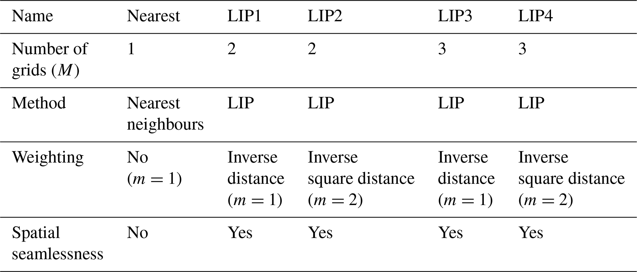
The parameters M and m are defined in Eq. (7).

In Eq. (3), dt is set to 1 h, which is an assumption and is tested by setting dt to 3–48 h (discussed in Sect. 4.2); dS is set to one grid, i.e. 1 km by 1 km, where the observation site is located. The ensemble size, N, is set to six, which is also tested by changing the number from six to two, three, four and five (discussed in Sect. 4.3). Hereafter, the proposed method is referred to as the “LMVE ensemble method”.

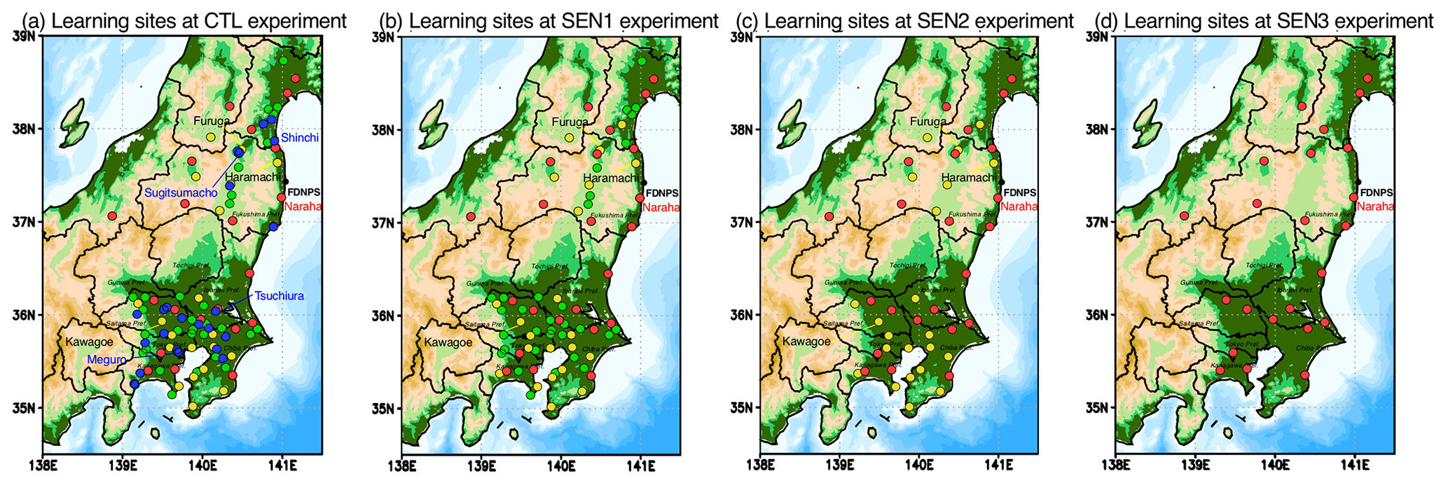
Figure 1 Cs-137 observation sites used as a learning site in (a) the standard (CTL), (b) SEN1, (c) SEN2 and (d) SEN3 experiments in this study. The closed black circle is the location of the FDNPS. The closed circles in red, yellow, green and blue are the locations of the learning data sites used in the CTL experiment. The closed circle in yellow is the learning data location used for the ensemble in CTL, SEN1 and SEN2. The closed circle in green is the learning data location used for the ensemble in CTL and SEN1. The closed circle in blue is the learning data location used for the ensemble in the CTL only. The number of sites is 23 (red), 22 (yellow), 32 (green) and 24 (blue). The details are also explained in Table 3. The words in italics are the names of prefectures. The Kantō region includes seven prefectures: Tokyo, Kanagawa, Chiba, Saitama, Ibaraki, Tochigi and Gunma. The background map for the elevation is obtained from the ETOPO (Amante and Eakins, 2009).

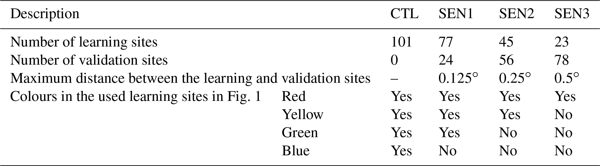
Table 3 Test experiments in the ensemble method using the selected sites.

2.3 Observation data

The hourly measured Cs-137 concentrations at the surface are directly estimated by using the aerosol sampling tapes of the national suspended particulate matter (SPM) network (Tsuruta et al., 2014, 2018). There are almost 400 SPM sites in eastern Japan, but now 101 sites have available data for Cs-137 (Oura et al., 2015). In this study, the measured Cs-137 data at 100 sites (one site, Futaba, was eliminated because the site is located in the same model grid as FDNPS, which is known as the change-of-support problem; Gotway and Young, 2002) are used for the ensemble. In addition, at an extra site, Tokai (36.45^∘ N, 140.59^∘ E), which covers the missing area of Oura et al. (2015), daily measured Cs-137 concentrations (Furuta et al., 2011) are used. All 101 sites used in this study are plotted using four different colours in Fig. 1. All measurements shown in Fig. 1 (all colour sites) are used as learning data in the LMVE ensemble method as a control experiment (CTL). In the sensitivity tests discussed in Sect. 4, we used all observation sites.

The colours represent the sites used to learn or validate the data in the extra ensemble estimation to examine the effect of the spatial interpolation for the σ² value on the MME concentrations. In the test experiments (SEN1, SEN2 and SEN3), some of the datasets are used as learning data and others are used as validation data, as shown in Table 3. The validation data are selected by choosing the sites with the largest number of observed samples as the representative site in the specific domain. When the specific domain is defined by a lattice of 0.125^∘ by 0.125^∘, the sites in yellow are used as validation data for the experiments (SEN3). When the specific domain is defined as a lattice of 0.25^∘ by 0.25^∘, the sites in yellow and green are used as validation data in the experiments (SEN2 and SEN3, respectively). When the specific domain is defined as a lattice of 0.5^∘ by 0.5^∘, the sites in yellow, green and blue are used as validation data for the experiments (SEN1, SEN2 and SEN3). This means that in the SEN2 experiment, the 56 sites in blue and green can be used as validation data, whereas the 45 sites in red and yellow are used as learning data. Since the area where Cs-137 is emitted from is the point source of FDNPS, a method used to randomly choose the learning/validation sites is not applied for accurately evaluating the spatial interpolation of the ensemble method.

2.4 Statistic metrics for the MME evaluation

The model evaluation should be carried out using multiple statistical metrics (e.g. Chang and Hanna, 2004). In this study, we introduce the geometric mean bias (GMB), root mean square error (RMSE) using the geometric variance (GV), Pearson correlation coefficient (PCC), and the fraction of data within a factor of 2 of observations (FAC2):

$$\begin{array}{}\text{(8)}& {\displaystyle }\mathrm{GMB}=\exp \left(\stackrel{\mathrm{‾}}{\log C_{\mathrm{obs}}}-\stackrel{\mathrm{‾}}{\log C_{\mathrm{sim}}}\right)\text{(9)}& {\displaystyle }\mathrm{RMSE}=\ln \left({\mathrm{GV}}^{\mathrm{2}}\right)\text{(10)}& {\displaystyle }\mathrm{GV}=\exp \left\{\stackrel{\mathrm{‾}}{{\left(\log C_{\mathrm{obs}}-\log C_{\mathrm{sim}}\right)}^{\mathrm{2}}}\right\}\text{(11)}& {\displaystyle }\mathrm{PCC}={\displaystyle \frac{\sum \left(\log C_{\mathrm{obs}}-\log \stackrel{\mathrm{‾}}{C_{\mathrm{obs}}}\right)\left(\log C_{\mathrm{sim}}-\log \stackrel{\mathrm{‾}}{C_{\mathrm{sim}}}\right)}{\sqrt{\sum {\left(\log C_{\mathrm{obs}}-\log \stackrel{\mathrm{‾}}{C_{\mathrm{obs}}}\right)}^{\mathrm{2}}\sum {\left(\log C_{\mathrm{sim}}-\log \stackrel{\mathrm{‾}}{C_{\mathrm{sim}}}\right)}^{\mathrm{2}}}}}\text{(12)}& {\displaystyle }\begin{array}{rl}\mathrm{FAC}\mathrm{2}& =\text{fraction\hspace{0.17em} of\hspace{0.17em} data\hspace{0.17em} that\hspace{0.17em} satisfy};\\ & \mathrm{0.5}\le {\displaystyle \frac{\log C_{\mathrm{sim}}}{\log C_{\mathrm{obs}}}}\le \mathrm{2.0}.\end{array}\end{array}$$

Because Cs-137 concentrations vary by several orders (e.g. Tsuruta et al., 2014), GMB and GV are preferred over the fractional bias method because they are suitable for extreme high and low values (Chang and Hanna, 2004). The RMSE is an indicator of uncertainty. In this study, the PCC is estimated using logarithmically scaled Cs-137 concentrations. Because the logarithmic Cs-137 is undefined for zero values, a minimum threshold of logarithmic Cs-137 is set to the lower threshold in the measurement, i.e. 0.01 Bq m⁻³. The PCC using logarithmically scaled values is actually not a robust measure because the lower limitation is sensitive to the results. However, the PCC using logarithmically scaled values is a useful indicator because it becomes applicable even for highly skewed distributions; therefore, we also use the PCC for the model evaluation. FAC2 becomes the most flexible metric for evaluating the model results even if its probability distribution frequency is highly skewed, and it can be an indicator of precision. These statistical metrics are calculated for the case in which the observed Cs-137 exceeds the detection limit. The total sampling number is 7056 for all available sites and times in the CTL experiment, whereas it is 1865 (minimum value) for the SEN1 experiment. Because the sampling number is adequately large, a direct comparison of these statistical metrics among the different experiments can be performed.

Figure 2 Temporal variations in Cs-137 at the relevant sites (Naraha, Haramachi, Furuga and Kawagoe). The locations in brackets represent the names of prefectures. The results are shown for the observations (“obs” in black), ensemble members (W1, W2, W3, W4, N1 and N2 in colours) and the ensemble model (red). The time is JST.

3 Results

3.1 LMVE ensemble method using all available observations

Cs-137 simulated by parts of the ensemble six members, i.e. W1 and N1, is evaluated under an MIP (Sato et al., 2018). The performances of these two members are moderate among the MIP-participating models. Here, all of the ensemble members and the ensemble results are compared with the measurements of the surface Cs-137 concentrations. Figure 2 shows the temporal variation in both simulated and observed Cs-137 at the sites near FDNPS and in the Kantō region. Generally, the ensemble results at these sites are the closest to the observations compared to the results of the single-member model. For example, at Naraha (Fig. 2a), which is the closest site to FDNPS, the first and second largest peaks in the observed Cs-137 are noteworthy during 15–17 March. The results of the ensemble members are largely dispersed, so the ensemble results become very close to the observations. In the other peaks, such as those on 16 and 20–21 March at Furukawa (Fig. 2c), the ensemble results are almost completely matched with the observations. However, the ensemble results are not close to the observations when all the results of the ensemble members are underestimated compared to the observation, as is the case on 13 March at Haramachi (Fig. 2b). In this case, the ensemble result has a peak on 12 March, which is earlier than the timing captured by the observation. In contrast, on 12 March at Naraha, some of the members have a peak in the simulated Cs-137; thus, the ensemble result also has a small peak, whereas the observation does not have such a peak. These cases are also shown on 20 March at Kawagoe (Fig. 2d), which can be explained as follows: when the Cs-137 simulated by all members is underestimated compared to the observations, the variance in Cs-137 between the observations and the simulations, as defined in Eq. (3), must be too large, and thus the weighted coefficient of the members, as defined in Eq. (5), becomes very small. Because the cross terms of the Cs-137 concentration and the weighted coefficient are small, the Cs-137 concentrations estimated by the ensemble must be underestimated. In contrast, when Cs-137 simulated by some members is overestimated compared to the observations, the weighted coefficient becomes very small. However, because the cross terms of the Cs-137 concentration and the weighted coefficient are not small, the Cs-137 concentrations estimated by the ensemble are overestimated, which represents one of the disadvantages of the LMVE ensemble method and prevents it from obtaining more accurate ensemble results relative to the observations.

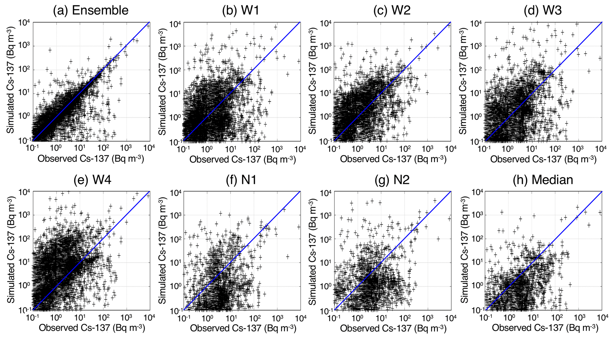
Figure 3 Relationship between the simulated Cs-137 and the observed Cs-137 at all available sites using the (a) ensemble model with all models (W1, W2, W3, W4, N1 and N2), (b–g) original one-member model (W1, W2, W3, W4, N1 and N2) and (h) median model using all models (W1, W2, W3, W4, N1 and N2). The blue line is the 1:1 line.

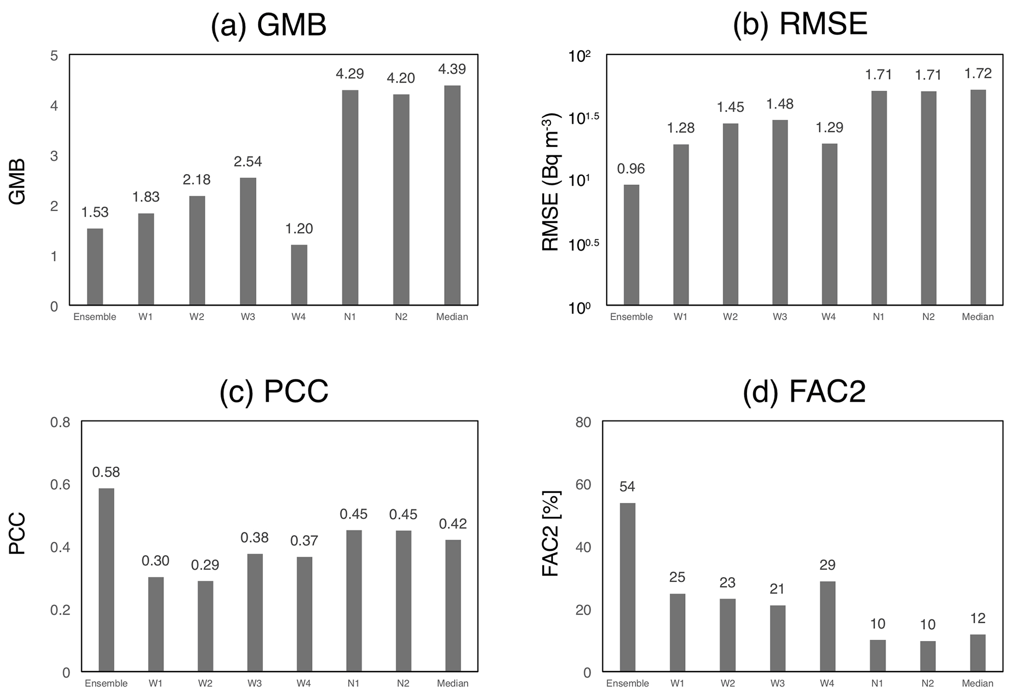
Figure 4 Statistical metrics defined in Sect. 2.4 using the simulated Cs-137 and observed Cs-137 at the available 101 sites. The metrics show the (a) GMB, (b) RMSE, (c) PCC and (d) FAC2. The results correspond to Fig. 3.

Figure 3 shows scatterplots for the observed and simulated Cs-137 at all sites using the ensemble results (a), the results of each member (b–g) and the median results (h) among the ensemble members. The statistical metrics are listed in Fig. 4, including the bias (GMB), uncertainty (RMSE), correlation (PCC) and FAC2. The perfect model presents values of GMB =1 (C_sim=C_obs), RMSE =0 Bq m⁻³, PCC =1 and FAC2 =1 (100 %). The observation values at all 101 sites are used in the LMVE ensemble method as learning data. Compared with the results of the other ensemble members, the ensemble result is the closest to the observations, with GMB =1.53, RMSE =10^1.709 (=9.42) Bq m⁻³ (i.e. the lowest uncertainty), PCC =0.59 and FAC2 =54 %. The ensemble members produce slightly overestimated results ranging from GMB =1.21 to GMB =2.54 (for W1, W2, W3 and W4) and considerably overestimated results ranging from GMB =4.20 to GMB =4.30 (for N1 and N2), and they have low to moderate correlations ranging from PCC =0.29 to PCC =0.45 and uncertainties ranging from 10^1.283 (=19.2) to 10^1.709 (=51.2) Bq m⁻³. The median result using all ensemble members has a moderate correlation of PCC =0.42 but a high GMB of 4.39 and high RMSE of 10^1.717 (=50.7) Bq m⁻³. The median and average values using many members is generally close to the best estimate compared to the original models (e.g. Draxler et al., 2015), although in this study, the median among the six members does not provide the best results.

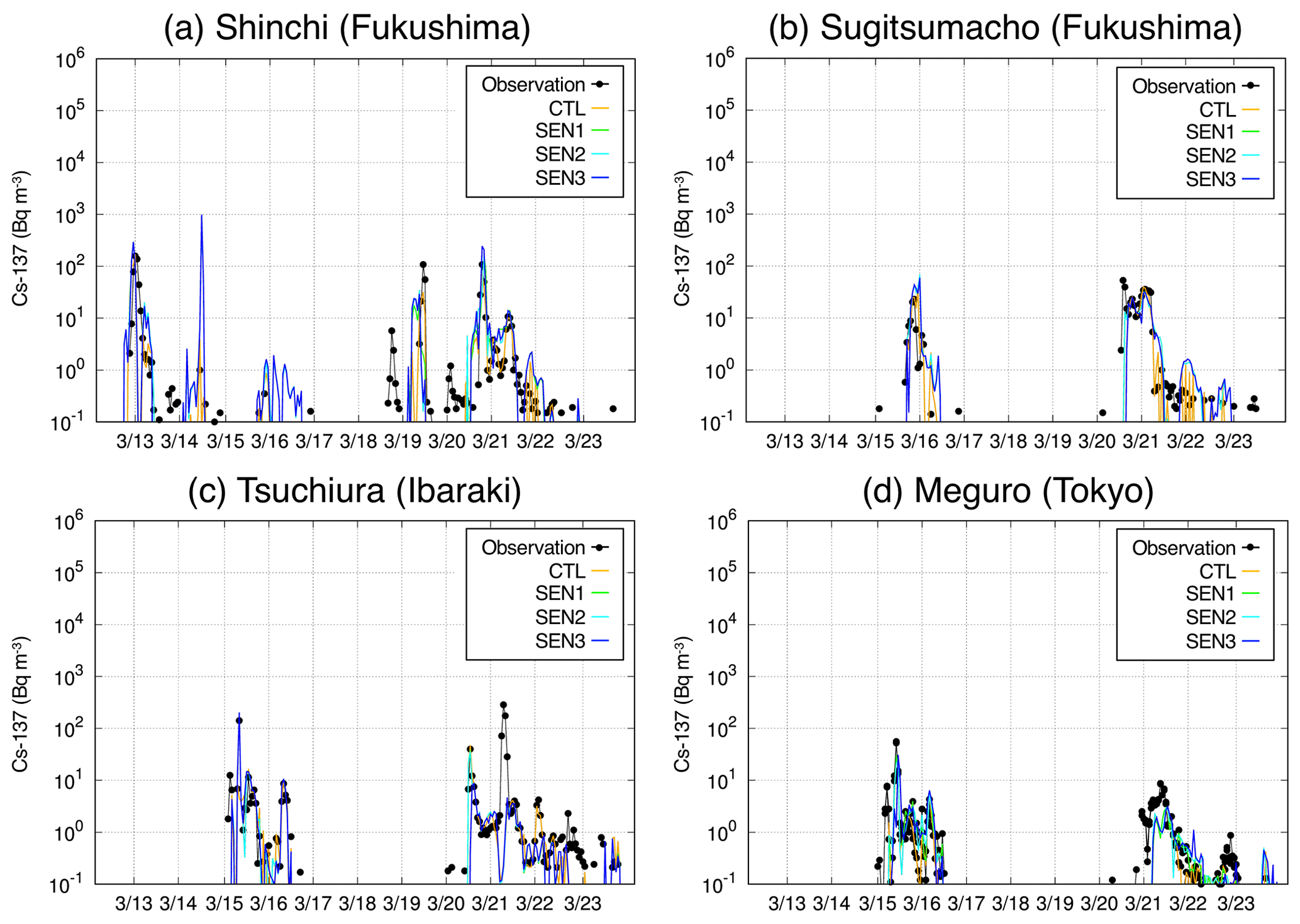
Figure 5 Temporal variations in Cs-137 at the independent sites (not learning but validation sites) using the LMVE ensemble method for CTL, SEN1, SEN2 and SEN3. The time is JST.

3.2 LMVE ensemble method using limited observations

In Sect. 3.1, the results of the CTL are shown, and in this section, the sensitivity tests (SEN1, SEN2 and SEN3 as shown in Sect. 2.3) for the separation of learning and validation sites are conducted. The test results are evaluated at the sites that are independent (used as validation data) from the other sites (used as learning data) in the LMVE ensemble method (Table 3). At the independent sites, the temporal variations in the simulated Cs-137 are compared at the four sites near FDNPS and in the Kantō region (Fig. 5). The sensitivity depends on the location; the results of all sensitivity tests (SEN1, SEN2 and SEN3) are sometimes far from the observations at Fukushima, as shown in Fig. 5a and b, whereas those of all the sensitivity tests (SEN1, SEN2 and SEN3) are generally close to the observations at the sites in the Kantō region (Fig. 5c and d). This suggests that the interpolation of variance (and thus the Cs-137 concentrations) near the FDNPS is sometimes not applicable, which is probably because the plume of high-density Cs-137 near the FDNPS is very narrow and strongly depends on local winds (Nakajima et al., 2017). The wind, especially low wind speeds, tends to influence the results at the observation sites (Weil et al., 1992).

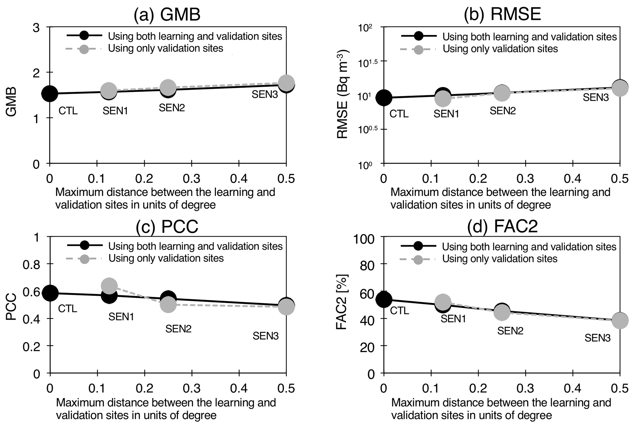
Figure 6 Statistical metrics (GMB, RMSE, PCC and FAC2) at the available sites for CTL, SEN1, SEN2 and SEN3. The statistical metrics are calculated using all sites (in black) and the independent sites (in grey), which are not used in the LMVE ensemble method. The names of the experiments are shown in each panel. The x axis represents a maximum distance between the learning and validation sites in units of degrees.

Figure 6 summarizes the statistical metrics among the sensitivity tests. This figure indicates that the GMB and RMSE values are larger and the PCC and FAC2 values are smaller as the distance between the learning and validation sites increases. The figure also shows that the differences in these metrics between the results using all and independent sites are small and thus clearly show the success of the linear interpolation of variance between the simulation and the observation in the LMVE ensemble method. These results are consistent with the results shown in the Kantō region of Fig. 5c and d, indicating that the largely spread plumes are generally reproduced by the ensemble method. As shown in Fig. 6, the relationship between the two axes, i.e. distance vs. PCC, can be fitted as a linear line with a slope of 0.18 for the results using all sites and 0.36 for the results using only the validation sites. The slope indicates that the PCC decreases by 0.02–0.04 when the distance from the learning site to the validation site increases by 0.1^∘. According to the approximate line, the distance is calculated to be 1.03^∘ when all sites are used and 0.68^∘ when the independent sites are used to obtain moderate correlation (PCC > 0.4). Therefore, the proposed interpolation is generally applicable for the best estimation within a distance of 0.7–1.0^∘, i.e. at least 70 km, from the observation site.

4 Discussion

This section discusses the uncertainties caused by several assumptions in the LMVE ensemble method. As described in Sect. 2.2, the spatial interpolation of variance defined in Eq. (3) assumes IDW. The selection of the sites is also uncertain and is investigated in Sect. 4.1. The time window used in Eq. (3) is assumed to be 1 h, which is discussed in Sect. 4.2. The ensemble size defined in Eqs. (4) and (5) is also discussed in Sect. 4.3. In Sect. 4.4, the spatial distribution of the Cs-137 surface concentrations estimated by the LMVE ensemble method is shown as an example for estimating the impact of Cs-137 on inhalation exposure of residents in Japan.

Figure 7 Statistical metrics (GMB, RMSE, PCC and FAC2) for the three sensitivity tests (SEN1, SEN2 and SEN3) as described in Table 3 using the five interpolation methods (nearest, LIP1, LIP2, LIP3 and LIP4) described in Table 2. The x axis represents the sensitivity experiments with the sampling number (N).

4.1 Sensitivity of spatial interpolation

The spatial interpolation of variance defined in Eq. (3) adopts IDW using two of the nearest sites as denoted by LIP1 in Table 2. Here, four extra methods in Table 2 are used for testing SEN1, SEN2 and SEN3, as shown in Sect. 3.2. Figure 7 illustrates the statistical metrics for 15 tests using the validation sites, which are not used in the LMVE ensemble method as learning data. For SEN1, all metrics in the five interpolation methods are estimated as 1.60±0.01 for GMB, 10^0.95±0.00 Bq m⁻³ for RMSE, 0.64±0.00 for PCC and 52±0.0 % for FAC2 by using 1865 data samples. The differences among the interpolation methods are close to zero. In SEN2 and SEN3, however, the differences among the five interpolation methods, especially between the nearest neighbours (named “nearest” in Table 2) and the others, become slightly larger than the others. The largest difference is observed between nearest and the others at 0.01 for GMB, 10^0.01 Bq m⁻³ for RMSE, 0.01 for PCC and 1 % for FAC2. Judging from the slight differences and the simplest method, we use the LIP1 method (using the two nearest sites and the weighting coefficient of the inverse distance) in the standard experiment. It should be noted that other interpolations were considered in the discussion, although they provided much worse results than those shown in Fig. 7 (not shown). The method that used the covariance between the observations at the nearest observation site and the simulation at the target grid was not applicable to this study because the covariance values are generally negative or close to zero at most grids due to the heterogenous distribution of Cs-137. Another method that uses all sites (not two or three grids) for the interpolation was also not applicable to this study because the influence of the ensemble coefficients at the grids far from the target grid cannot be ignored.

Figure 8 Same as Fig. 2 except for the use of the ensemble results with various time windows ranging from 1 h (tw01hr) to 49 h (tw49hr).

4.2 Sensitivity of the time window

To investigate the sensitivity of the time window in Eq. (3), the temporal variations in Cs-137 simulated by the ensemble methods are shown in Fig. 8 using various time windows ranging from 1 to 49 h (not all results are shown in Fig. 8). The difference in the estimated Cs-137 concentrations is generally small but sometimes very large. In Fig. 8a, for example, at Naraha on 20 March, the observed peak is sharp, whereas the sharpness of the estimated peaks depends on the time window values. As the time window increases, the sharpness of the peak becomes weak, i.e. the peak is broadly distributed. At Kawagoe (Fig. 8d) on 20–22 March, the estimated Cs-137 concentrations using the longer time window are far from the observations and estimations using the shorter time window. Such situations are found at the other sites and during other periods (not shown). This also indicates that the peak in Cs-137 is very sharp temporally and spatially, so the time window must be shortened. The dependency of the time window on the results is investigated using the statistical metrics at all sites used in the LMVE ensemble method, as shown in Fig. 9. The dependency of the time window on the GMB, RMSE, PCC and FAC2 was found to be strong; moreover a shorter time window tends to provide higher PCC and FAC2 values and lower GMB and RMSE values. Therefore, the time window in the standard experiment is set to the shortest time, i.e. 1 h.

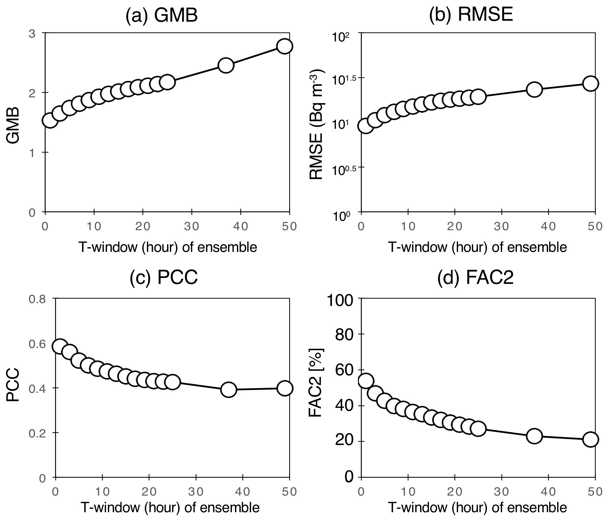
Figure 9 Statistical metrics (GMB, RMSE, PCC and FAC2) at the 101 available sites against various time windows (x axis) ranging from 1 to 49 h.

4.3 Sensitivity of the ensemble size

The previous study of Nakajima et al. (2017) used only two members for the LMVE ensemble method, and the ensemble results were better than the original results for each member, but the difference in the PCC was very small (0.03–0.05; Table 1 in Nakajima et al., 2017). Therefore, this study increases the number of LMVE ensembles to six members and investigates the sensitivity of the ensemble size to the results. Figure 10 shows the relationship between the ensemble size and the statistical metrics (GMB, RMSE, PCC and FAC2). The results clearly show that as the ensemble size increases, the GMB and RMSE decrease, and the PCC and FAC2 increase. This tendency can also be found in previous studies (e.g. Pennell and Reichler, 2010; Kioutsioukis and Galmarini, 2014; Solazzo and Galmarini, 2015a). Using two members, the average GMB is calculated to be 1.95, which is smaller than that obtained using a single member by 0.76; the average RMSE is calculated to be 10^1.208 (=16.2) Bq m⁻³, which is smaller than that obtained using a single member by 10^1.155 (=14.3) Bq m⁻³; the average PCC is calculated to be 0.46, which is larger than that obtained using a single member by 0.08; and the average FAC2 is calculated to be 34 %, which is larger than that obtained using a single member by 14 %. Using more than two members, the PCC is calculated to be more than 0.4, i.e. a moderate correlation. Using five members, the average GMB is calculated to be 1.56, which is larger than the value of 1.53 obtained using six members; the average RMSE is calculated to be 10^0.984 (=9.63) Bq m⁻³, which is larger than the value of 10^0.960 (=9.12) Bq m⁻³ obtained using six members; the average PCC is calculated to be 0.57, which is smaller than the value of 0.59 obtained using six members; and the average FAC2 is calculated to be 51 %, smaller than the value of 54 % obtained using six members. However, the best ensemble results obtained using five members are close to those obtained using six members, with differences of +0.1 % for GMB, +1.5 % for PCC, +0.0 % for RMSE and +0.2 % for FAC2. By contrast, the best ensemble results obtained using four members are worse than those obtained using six members, with the differences of −1.6 % for GMB, −0.9 % for PCC, +0.8 % for RMSE and −4.0 % for FAC2. Therefore, we conclude that the minimum number in the LMVE ensemble in this study is five but only when the members are effectively selected. When the members cannot be selected, the best results can be obtained by reducing the weighting coefficients of the members through the calculation of the LMVE method, since the difference in the statistical metrics between six- and five-member ensembles is very small.

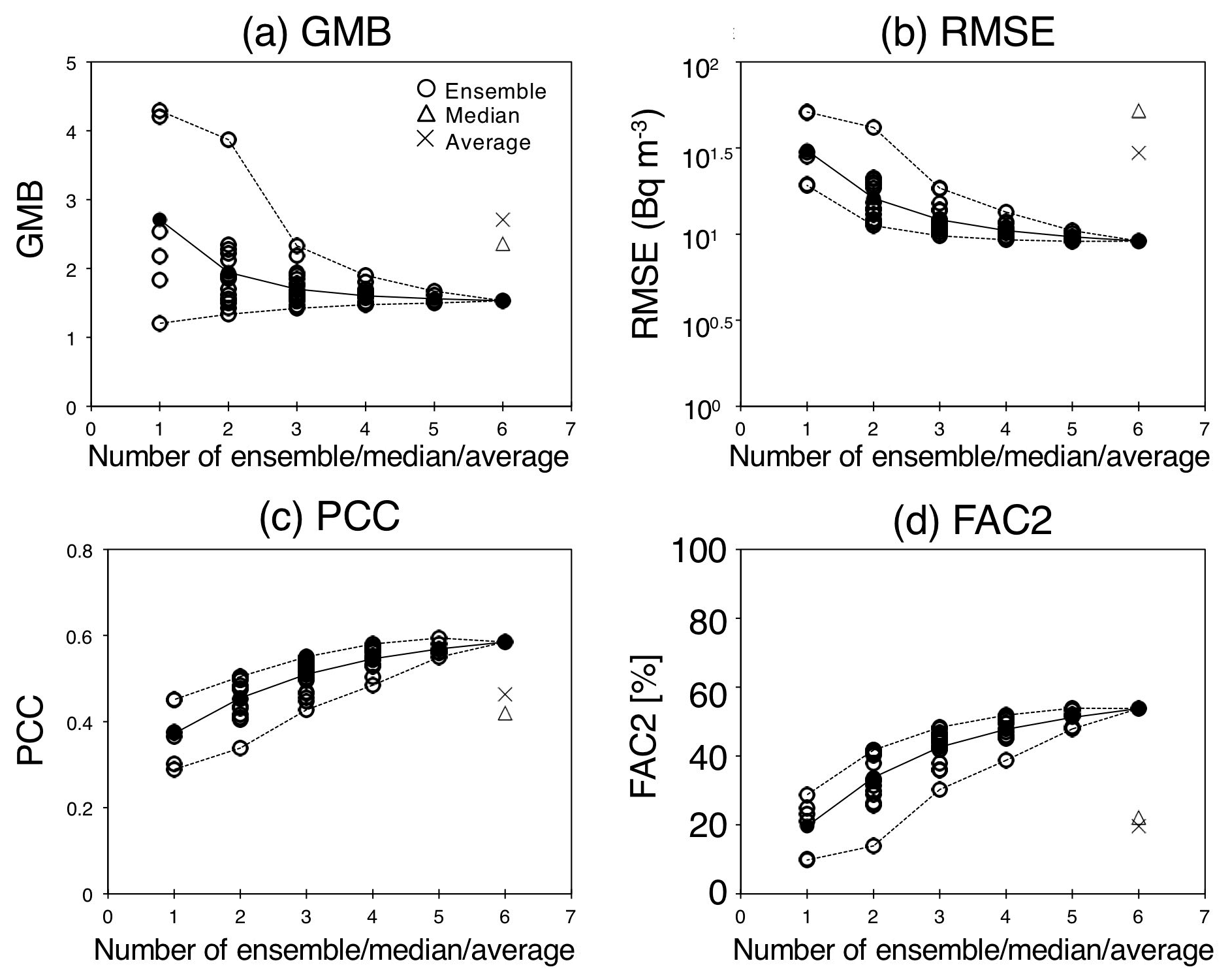
Figure 10 Statistical metrics (GMB, RMSE, PCC and FAC2) at the available sites against the number of the ensemble members, the median and the average (x axis). The black line indicates an average of the ensemble results for each number, whereas the dashed line indicates the maximum and minimum results of the ensemble results for each number.

Even in the best estimate using selected five or six members, the PCC value is less than 0.7, which means the ensemble results are moderately (not strongly) correlated with the observations. Therefore, to obtain values much closer to the observations, a new ensemble member is required. As explained in Sect. 3.1, when one of the members provides results close to the observations even at 1 h, the ensemble results proposed in this study become closer to the observations.

For the median and average values using six members, the PCC is calculated to be 0.42 and 0.46, respectively, similar to the ensemble results obtained using two members. By contrast, the GMB, RMSE and FAC2 values for the median and average results obtained using six members are close to the results for the single members. Since the median and average values obtained using many members are generally closer to the best estimate compared to the original members, the original members used in this study are not independent of each other. Therefore, these results indicate that the LMVE ensemble method is applicable even when the ensemble size is only two and even when they are not independent, although the bias, uncertainty, correlation and precision dramatically decrease as the ensemble size increases. The proposed ensemble method is very useful for properly estimating Cs-137 concentrations, even under a limited ensemble size.

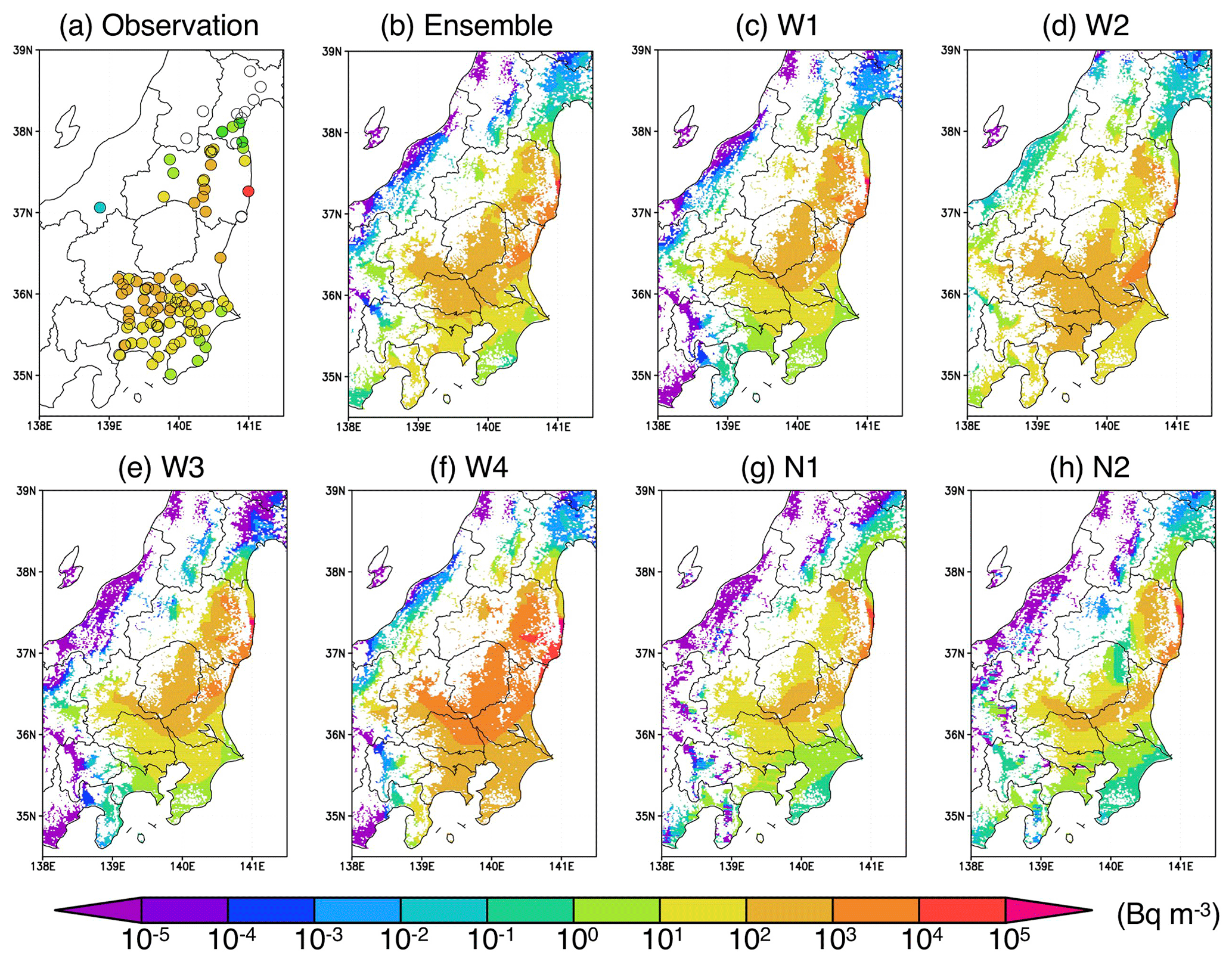
Figure 11 Spatial distribution of the (a) observed and (b–h) simulated daily integrated Cs-137 concentrations on 15 March 2011 (JST).

4.4 Cs-137 spatial distribution

The above discussion indicates that the LMVE ensemble method can better estimate the Cs-137 distribution; the spatial distributions of Cs-137 concentrations that are integrated daily on 15 March 2011 are also shown (Fig. 11). In the Fukushima prefecture, including the FDNPS, the results of Cs-137 simulated by each member are largely spread, so the ensemble results, especially in the area far from the observation sites, are very important. Figure 5 suggests that the ensemble results are moderately correlated with the observations around the area where the distance from the observation site is approximately 20–30 km. Therefore, in the Fukushima prefecture, which presents a complex terrain, parts of the results of Cs-137 in this area are still uncertain, even when using models with a 3 km horizontal grid, because part of the area is far (30 km away the coast of Fukushima, which is called Hama-dori in Japan), and the inner area is the location of many observation sites (called Naka-dori in Japan). By contrast, although the difference in the simulated plumes among each member is very large over the Kantō region, the conclusion from Sect. 3.2 supports the results that the ensemble Cs-137 results are closer to the observations, with PCC > 0.4, compared to the results of each member. This result is obtained because in the Kantō region, most areas are within 70 km of any observation site. However, some of the prefectures in the Kantō region do not have measurement sites, so in these prefectures, the ensemble results are still uncertain. This suggests that in the future, it should be required to observe Cs-137 at distance intervals of 20–30 km distance near the source region and 70 km in other areas to properly estimate the best results of the Cs-137 spatial distribution.

5 Conclusions

The LMVE ensemble method is based on a classical idea but is still useful for estimating the best results using MMEs and observations without requiring a large amount of computer resources for high-resolution models. This method was first applied to estimate the Cs-137 distribution by Nakajima et al. (2017) and is extended in this study. The uniqueness of this approach compared with other MMEs for other species is based on the following: (1) the availability of observed Cs-137 concentrations near the surface at approximately 100 sites, thus providing dense coverage over eastern Japan; (2) the simplicity of identifying the emission source of Cs-137 associated with the point source of FDNPS; (3) the novelty of implementing the MME approach with a high-resolution model over complex terrain in eastern Japan; and (4) the strong need to better estimate the Cs-137 distribution due to its inhalation exposure risk among residents in Japan. However, Nakajima et al. (2017) did not thoroughly discuss the availability of this method in depth, show the biases, uncertainties, precision and generalizability of this method under varying time windows, space windows and ensemble sizes. Radioactive Cs-137 was released from the FDNPS in March 2011, and many studies have investigated the distribution of Cs-137, but the proper estimations of Cs-137 are not still adequate. Therefore, this study first extended the LMVE ensemble method to an ensemble size of six for simulating Cs-137, including two models, the WRF-CMAQ and NICAM models, and observations and then investigated their uncertainties to confirm their performances to generalize this method and attempt to give the best estimate for the estimation of their inhalation impacts on humans, which is a companion study by Takagi et al. (2020). The results of the ensemble members are also updated from Nakajima et al. (2017) by using a finer horizontal resolution (3 km grid) and by nudging an improved meteorological field provided by Sekiyama et al. (2017).

The proposed LMVE ensemble method provides the best results among the single members of the ensemble. This shows that the MME-estimated Cs-137 concentrations at all available 101 sites have the lowest bias against the observations, with GMB =1.53; the lowest uncertainties, with RMSE =9.42 Bq m⁻³; the highest correlation against the observations, with PCC =0.58; and the highest precision against the observations, with FAC2 =54 %. Moreover, the single-model members provided higher biases (GMB =1.83–4.29, except for 1.20 obtained from one member), higher uncertainties (RMSE =19.2–51.2 Bq m⁻³), lower correlation coefficients (PCC =0.29–0.45) and lower precision (FAC2 =10 %–29 %). In the model grid excluding the observations, Cs-137 is estimated by a spatial interpolation of variance in the formulation of the LMVE using the inverse distance weighting between the nearest two sites. For the test of this assumption, the available measurements are divided into two sets, learning and validation data, and thus the test finds that the assumption for linear interpolation promises a moderate PCC value (> 0.4) within a distance of 0.7–1.0^∘, i.e. at least 70 km. Extra sensitivity tests for several parameters, i.e. the site number and the weighting coefficients in the spatial interpolation, the time window in the LMVE and the ensemble size, are determined. As a result, the findings for the uncertainty in the proposed LMVE ensemble method are shown. (1) The LIP1 method (using two sites and IDW) is the simplest and provides better results than the other interpolations. (2) The time window in the LMVE ensemble method can be set to 1 h. (3) A larger number of ensemble members (ensemble size) remarkably yielded better results, and having more than two members generates better results than each member alone, even when the members are not completely independent. In this study, the minimum ensemble size is found to be five, but only when the members are effectively selected. The best ensemble size can be six if the weighting coefficient of the member is minimized through the LMVE calculation without selecting any members.

It should be noted, however, that the LMVE ensemble method presents certain limitations. When Cs-137 simulated by all members is too underestimated compared to the observations, the variance in Cs-137 between the observations and the simulations, as defined in Eq. (3), must be too large, and thus the weighted coefficient of the members, as defined in Eq. (5), becomes very small. Because the cross terms of the Cs-137 concentration and the weighted coefficient are small, the Cs-137 concentrations estimated by the ensemble must be underestimated. By contrast, when Cs-137 is overestimated by some members, the weighted coefficient becomes very small. However, because the cross terms of the Cs-137 concentration and the weighted coefficient are not small, the Cs-137 concentrations estimated by the ensemble are overestimated.

In addition, the spatial interpolation used in this study does not obtain a moderate PCC value (> 0.4) in the areas where the distance from the observation sites exceeds approximately 70 km. Therefore, the estimated results over the area with very sporadic site locations are very uncertain, especially for the inner areas of the Kantō region, e.g. Gunma and Tochigi prefectures. The assumption of the spatial interpolation using IDW is difficult to apply to broadly distributed materials, such as Cs-137 emitted from the FDNPS, which is spatially and temporally distributed very heterogeneously (Nakajima et al., 2017). It can be said that it is difficult to use any spatial interpolation, which basically assumes the spatial smoothness of the target's concentrations based on the best estimation of the Cs-137 distribution. In the future, Cs-137 should be observed at distance intervals of 20–30 km near the source region, including in complex terrain, and at intervals of at least 70 km in other areas to properly estimate the best results of the Cs-137 spatial distribution.

This study only applies the LMVE ensemble method to radioactive Cs-137 in the atmosphere, but this method can be applied to Cs-137 deposition and atmospheric pollutants, such as PM_2.5. However, the results obtained in this study are not directly used for estimation of the best estimate of the Cs-137 deposition because the simulated Cs-137 concentration and the simulated Cs-137 deposition flux are not generally correlated with each other, as suggested by previous model comparison studies (Kitayama et al., 2018). Recently, large areal coverage of surface PM_2.5 measurements has become available for most countries (https://aqicn.org/map/world/, (last access: 6 March 2020). In addition, since the PM_2.5 distribution does not vary abruptly, the LMVE ensemble method is easily applied for PM_2.5 estimations. Therefore, this method will be applied in our future study to estimate the PM_2.5 distribution for better air quality prediction.