Statistical analysis of ice microphysical properties in tropical mesoscale convective systems derived from cloud radar and in situ microphysical observations

This study presents a statistical analysis of the properties of ice hydrometeors in tropical mesoscale convective systems observed during four different aircraft campaigns. Among the instruments on board the aircraft, we focus on the synergy of a 94 GHz cloud radar and two optical array probes (OAP; measuring hydrometeor sizes from 10 µm to about 1 cm). For two campaigns, an accurate simultaneous measurement of the ice water content is available, while for the two others, ice water content is retrieved from the synergy of the radar reflectivity measurements and hydrometeor size and morphological retrievals from OAP probes. The statistics of ice hydrometeor properties are calculated as a function of radar reflectivity factor measurement percentiles and temperature. Hence, mesoscale convective systems (MCS) microphysical properties (ice water content, visible extinction, mass–size relationship coefficients, total concentrations, and second and third moments of hydrometeor size distribution) are sorted in temperature (and thus altitude) zones, and each individual campaign is subsequently analyzed with respect to median microphysical properties of the merged dataset (merging all four campaign datasets). The study demonstrates that ice water content (IWC), visible extinction, total crystal concentration, and the second and third moments of hydrometeor size distributions are similar in all four types of MCS for IWC larger than 0.1 g m⁻³. Finally, two parameterizations are developed for deep convective systems. The first concerns the calculation of the visible extinction as a function of temperature and ice water content. The second concerns the calculation of hydrometeor size distributions as a function of ice water content and temperature that can be used in numerical weather prediction.

1 Introduction

Defining clouds and how they interact with the atmosphere is a major challenge in climate sciences and meteorology. Clouds play an important role in the evolution of the weather and climate on Earth. They affect the dynamics and thermodynamics of the troposphere and impact the radiative transfer of energy in thermal and visible wavelengths by heating or cooling the atmosphere. In addition, clouds represent an important part of the hydrological cycle, due to evaporation and precipitation processes. Inversely, dynamic features such as the Madden–Julian oscillation (MJO, perturbation of large-scale circulation leading to an eastward propagation of organized convective activity) can also affect the development of deep convective clouds (Madden and Julian, 1994, 1971). Mesoscale convective systems (MCS) are complex clouds and are the result of specific synoptic conditions and mesoscale instabilities that lead to the development of cumulonimbus (Houze, 2004). The complexity of MCS also relies on the dynamical, radiative, and precipitative characteristics that depend on the location in the evolving MCS (Houze, 2004). MCS can last several hours and can affect human societies in different ways. Indeed, MCS are often associated with hazardous weather events such as landslides, flash floods, aircraft incidents, and tornadoes, all of which can cause loss of human lives.

Weather and climate models use rather simplified schemes to describe ice hydrometeor properties. Parametrization disagreements due to larger uncertainties in the representation of ice properties in clouds (Li et al., 2007, 2005) lead to large variations in the quantification of ice cloud effects on climate evolution (Intergovernmental Panel on Climate Change Fourth Assessment Report). An accurate estimation of the spatiotemporal distribution of ice water content (IWC) is a key parameter for evaluating and improving numerical weather prediction (Stephens et al., 2002). Underlying hydrometeor growth processes in MCS vary in time (growing, maturing, and decaying phase) but also in space, i.e., horizontally (distance from active convective zone) and vertically (as a function of temperature).

A number of studies (Gayet et al., 2012; Lawson et al., 2010; Stith et al., 2014) demonstrate the presence of different types of ice hydrometeors in evolving MCS. In the active convective area, supercooled droplets larger than 500 µm and up to 3 mm were observed near −4 ^∘C, and rimed ice hydrometeors about the same size were observed below −11 ^∘C. At −47 ^∘C, rimed particles about 2–3 mm from updraft regions coexisting with ice crystals about 100 µm (pristine ice) were also encountered. Near the convective zone of MCS (i.e., fresh anvil), presence of pristine ice (about 100 µm), aggregates of hexagonal plates (about 500 µm to 1 mm), and capped columns (about 500 µm) has been reported (Lawson et al., 2010). In aged anvils, columns (∼ 100 µm), plates (∼ 100 µm), and small aggregates (about 200 µm) are observed near −43 ^∘C, while large aggregates about 2 mm and larger are found at lower altitudes (−36 ^∘C). Additionally, in the cirrus part of MCS bullet rosettes that are about 500 µm and smaller (more common for in situ cirrus; Lawson et al., 2010) and chain-like aggregates from 100 µm up to about 1 mm are found (aggregates of small rimed droplets caused by electric fields; Gayet et al., 2012; Stith et al., 2014).

With respect to ice particle density, Heymsfield et al. (2010) reported that ice particles seem to be denser near the convective part of MCS formed during the African Monsoon. Other studies have shown a variability of the mass–size relationship with temperature and related altitude (Fontaine et al., 2014; Schmitt and Heymsfield, 2010), which appears to be essentially linked to the variability of ice hydrometeor shapes related to different growth regimes (vapor diffusion, riming, aggregation).

Due to the above-mentioned spatiotemporal variations in MCS, the different mean tendencies (hydrometeor concentration, ice water content, coefficients of mass–size relationship) reported in earlier studies can be partly linked to the chosen observation strategy of the MCS (i.e., flight track in MCS), which of course is related to the particular objectives of the respective field projects (e.g., improvement of rain rate retrieval from satellite observations, icing condition at high altitude, comparison with ground radar observations).

Therefore, the goal of this study is, on the one hand, to investigate the vertical variation in ice crystal properties in MCS (e.g., as a function of temperature) and, on the other hand, to study horizontal trends of ice microphysics at constant temperature levels. The latter will be accomplished by a composite analyses of microphysical properties and a simultaneously measured radar reflectivity factor (Z). This study is focused on ice microphysics in deep convective systems. A preliminary investigation of the impact of vertical velocity has been performed as well. However, no significant tendencies were found that allow us to present our results as a function of vertical velocity.

A frequency distribution of the profiles of the radar reflectivity factor throughout the MCS as a function of temperature allows us to divide the microphysical in situ measurements into eight zones. For these height reflectivity zones, microphysical properties are analyzed and compared between the eight zones but also intercompared between different locations and associated measurement campaigns where MCS were observed. Some direct applications of this study could be for the improvement of retrievals of cloud properties from passive and active remote sensing observations or parameterization of ice properties in weather and climate models for deep convective clouds. Moreover, it could help identify zones in MCS where numerical weather predictions fail to represent ice microphysics.

Our statistical analysis is performed on cloud radar Doppler measurements and in situ measurements. Cloud radar measurements include more than 1 million data points of radar reflectivity factors and retrieved vertical velocities spanning from 170 to 273.15 K (temperature profiles from Radar Aéroporté et Sol de Télédétection des Propriétés Nuageuse (RASTA) are calculated using reanalysis of ECMWF), and in situ measurements include 55844 data points of 5 s duration in the temperature range from 215 to 273.15 K. Section 2 describes the utilized datasets and their derived parameters used in this study. Section 3 presents the analysis of radar reflectivity factors (Z), which provides the ranges of Z for performing the intercomparison between the four types of MCS. Moreover, for each range of Z a statistical analysis of vertical velocity is presented to bind the vertical dynamics of MCS and ice microphysical properties. Section 4 presents the methodology of intercomparison used in this study. Section 5 presents the intercomparison of the microphysical parameters as a function of Z and T; the end of this section is dedicated to briefly presenting the results of the investigations performed into the impact of vertical velocity on the data. Section 6 provides the parameterization of visible extinction and the parameterization of ice hydrometeor distributions. Finally, Sect. 7 adds the discussion and conclusion.

2 Data description

This study uses a dataset where MCS were observed in four different locations in the tropics and related to two different projects.

1. Megha-Tropiques in Niamey, during July and August 2010: observation of continental MCS formed over the region of Niamey (Niger) during the West African Monsoon (Drigeard et al., 2015; Fontaine et al., 2014; Roca et al., 2015). These MCS developed over the continent (7665 in situ points of 5 s).

2. Megha-Tropiques in the Maldives, during November and December 2011: observation of oceanic MCS that developed over the southern part of the Maldives, related to the ITCZ (Intertropical Convergence Zone) in the Indian Ocean. (Fontaine et al., 2014; Martini et al., 2015; Roca et al., 2015). It includes MCS developed during the wet phase of the MJO and two events with isolated convective systems developed during the dry phase of the MJO (3347 in situ points of 5 s).

3. HAIC-HIWC in Darwin, from January to March 2014: observations of MCS formed over Darwin and the northeastern cost of Australia during the North Australian Monsoon (Leroy et al., 2016, 2017; Protat et al., 2016; Strapp et al., 2016b; Fontaine et al., 2017). During this campaign, MCS developed over the land, the ocean, and near the coast (23 265 in situ points of 5 s).

4. HAIC-HIWC in Cayenne during May 2015: observations of MCS developed over the French Guiana during the peak of its rainy season (Yost et al., 2018). In the same way as for Darwin, MCS developed over the land, the ocean, and near the coast (21 567 in situ points of 5 s).

Note that observations were essentially performed in mature MCS. All four measurement campaigns were conducted with the French research aircraft Falcon-20 operated by SAFIRE (Service des Avions Français Instrumentés pour la Recherche en Environnement). Two optical array probes (OAPs) were mounted on board the Falcon 20: the 2D-S (2-D stereographic probe; Lawson et al., 2006) and PIP (Precipitation Imaging Probe; Baumgardner et al., 2011), with the cloud radar RASTA operating at 94 GHz (Protat et al., 2016; Delanoë et al., 2014). In addition, bulk IWC measurements performed with the isokinetic evaporator probe (IKP-2 probe; Strapp et al., 2016a; Davison et al., 2010) were available for the HAIC-HIWC flight campaigns (Darwin and Cayenne).

Both OAP probes record black and white images of hydrometeors with a resolution of 10 and 100 µm (2D-S and PIP, respectively). They are used to derive the size of hydrometeors (D_max, in cm, in this study), their projected surface (S, in cm²), their concentrations (or particle size distribution, PSD) as a function of their size (N(D_max), in ${\mathrm{L}}^{-\mathrm{1}}\mathrm{\mu }{\mathrm{m}}^{-\mathrm{1}}$). The sizes of hydrometeors span from 10 µm to 1.28 cm, with D_max calculated as a function of the projected surface of hydrometeors (taking the maximum radius passing through its barycenter; see Fig. 1 in Leroy et al., 2016).

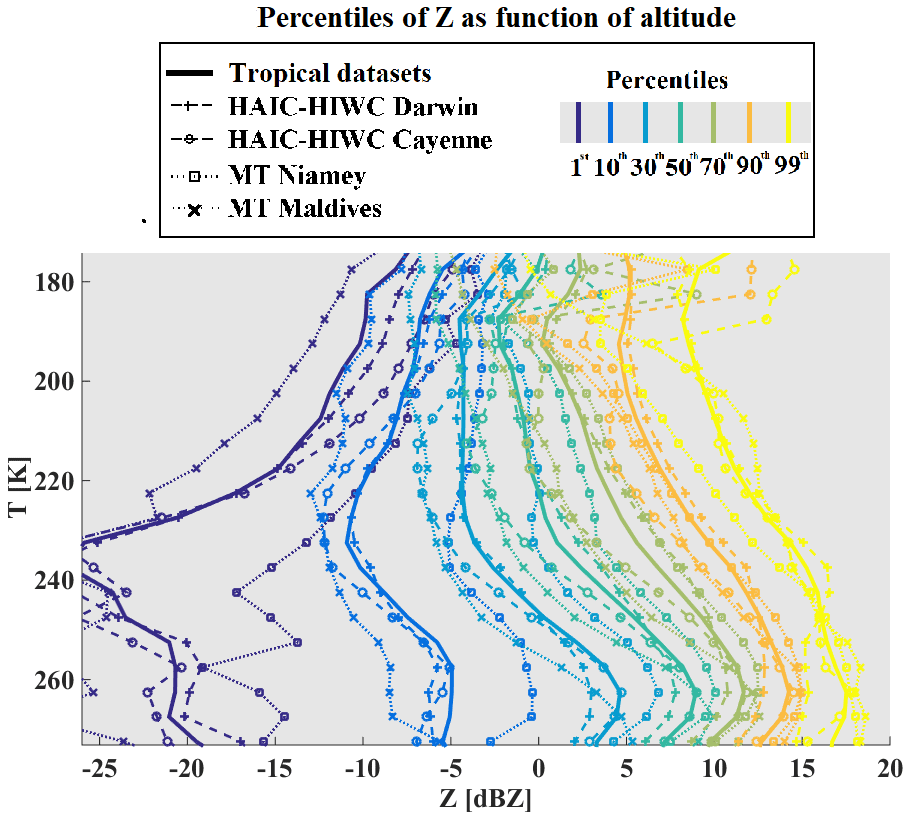
Figure 1 Percentiles of radar reflectivity factors in dBZ on x axis, as a function of temperature on y axis.

During both HAIC-HIWC campaigns, the IKP-2 probe was used to measure total condensed water, which was composed exclusively of ice water content (IWC, in g m⁻³) and water vapor, and IWC was then deduced using in situ measurements of relative humidity. However, IWCs < 0.1 g m⁻³ are not considered in this study, due to IKP-2 uncertainties that are particularly important for low IWC measurements (see Strapp et al., 2016a). For both Megha-Tropiques campaigns, IWC was retrieved using simulations of the reflectivity factor Z and images of OAP, thereby using the approximation of ice oblate spheroids (Fontaine et al., 2014, 2017). Results regarding the accuracy of IWC retrieved from this latter method with regards to IKP-2 measurement are discussed in Fontaine et al. (2017).

The 94 GHz RASTA radar measures Z and Doppler velocity V_d below and above the aircraft. RASTA has six antennas that allow for measuring three noncollinear Doppler velocities, from which the three wind components (including the vertical air velocity) have been reconstructed (using the Protat and Zawadzki, 1999, 3-D wind retrieval technique modified for aircraft geometry).

A detailed description of the data processing is documented in Leroy et al. (2016, 2017), Protat et al. (2016), Strapp et al. (2016b), and Davison et al. (2016). These references give a processing description for both datasets of the HAIC-HIWC project. However, the Megha-Tropiques datasets (Fontaine et al., 2014) were reprocessed in order to undergo exactly the same version of the processing tools in this study for comparison reasons.

Moreover, investigations have been performed to detect supercooled water using a Rosemount icing detector (Baumgardner and Rodi 1989; Claffey et al., 1995; Cober et al., 2001) and cloud droplet probe measurements. A few cases of supercooled water were detected and removed from the dataset (Leroy et al., 2016). Hence, the dataset used in this study exclusively uses data collected where only ice particles were measured. Additionally, retrieval of IWC for the Megha-Tropiques project was not performed in mixed-phase conditions (more details in Fontaine et al., 2014, 2017).

3 Radar observations

3.1 Radar reflectivity factors

In this section distributions of radar reflectivity factors Z from nadir and zenith profiles are investigated for the four datasets. Figure 1 shows percentiles of Z as a function of T measured with RASTA during the four airborne campaigns. The lines are color-coded as a function of the calculated percentiles. The percentiles of Z are calculated for a merged dataset that includes 11 flights for Megha-Tropiques (MT) over Niamey, 11 flights for MT over the Maldives, 19 flights for HAIC-HIWC over Darwin, and 17 flights for HAIC-HIWC over Cayenne. Percentiles are not calculated as a function of the number of profiles but by temperature ranges of 5 K, where only data with Z larger than −30 dBZ are taken into account. Figure 1 shows that distributions of Z are not totally similar for all four airborne campaigns. MCS can extend over hundreds or thousands of square kilometers, where size and distribution of their convective and stratiform areas can vary from one MCS to another. Hence, the same sampling strategy in two different MCS can provide two different statistics of ice microphysics properties as a function of T, just as two different sampling strategies in the same MCS can provide different results. The idea of this study is to compare the properties of ice hydrometeors for different tropical MCS locations, thereby rendering comparable different MCS systems (as a function of temperature) through the analysis of the frequency distribution of profiles of Z by dividing all MCS into eight zones. This strategy aims to reduce the impact of the different flight patterns and objectives for sampling MCS during each airborne campaign used in this study.

Note that Z at 94 GHz is linked to the ice water content (Fontaine et al., 2014; Protat et al., 2016) but also to the size distribution of ice hydrometeors, their respective crystal sizes, and their mean diameter (Delanoë et al., 2014).

Our motivation for choosing the limits of Z ranges from which the statistics of the ice hydrometeor properties are calculated holds is twofold. First, Fig. 1 shows that the variability of Z at a given T is large and that this variability of Z is due to altitude. We can observe in Fig. 1 that Z extends from about −20 to 18 dBZ at 260 K, while it spreads out from −10 to 10 dBZ at 200 K. These facts have to be considered if we want to sort our dataset as a function of T and Z. Therefore, the limit of the Z range cannot be the same for each altitude, as finding ice hydrometeors linked to 15 dBZ or −20 dBZ at 200 K is quite impossible. The second reason is due to the results of an earlier study. Cetrone and Houze (2009) used the profiling radar of TRMM satellite (Tropical Rainfall Measuring Mission; Huffman et al., 2007) to demonstrate with frequency distributions of radar reflectivity Z as a function of height that higher Z occur more often in convective echoes of MCS (in West African Monsoon, Maritime Continent and Bay of Bengal) than in their stratiform echoes. This earlier study was performed with the 13 GHz radar profiler on board the TRMM satellite, which is more sensitive to the precipitating particles (large drops and large ice crystals). The radar used in our study is more sensitive to smaller sizes of hydrometeors and linked to IWC (Protat et al., 2016). Thus, it is more adapted to sorting the properties of ice crystals presented in our study. Hence, this study presents ice microphysical properties in MCS as a function of temperature layers and as a function of zones of reflectivity Z. In order to fix the limits of a limited number of Z levels, this study takes the percentiles of all merged campaign datasets shown by the solid lines (all data) in Fig. 1. This defines Z ranges as a function of height. Hereafter, these ranges will be called MCS reflectivity zones (MCSRZ) and have been numbered from 1 to 8:

• MCS reflectivity zone 1: Z<Z^1st;

• MCS reflectivity zone 2 : $Z\in \left[Z\right(T{)}^{\mathrm{1}\text{st}};Z\left(T{)}^{\mathrm{10}\text{th}}\right[$;

• MCS reflectivity zone 3 : $Z\in \left[Z\right(T{)}^{\mathrm{10}\text{th}};Z\left(T{)}^{\mathrm{30}\text{th}}\right[$;

• MCS reflectivity zone 4 : $Z\in \left[Z\right(T{)}^{\mathrm{30}\text{th}};Z\left(T{)}^{\mathrm{50}\text{th}}\right[$;

• MCS reflectivity zone 5 : $Z\in \left[Z\right(T{)}^{\mathrm{50}\text{th}};Z\left(T{)}^{\mathrm{70}\text{th}}\right[$;

• MCS reflectivity zone 6 : $Z\in \left[Z\right(T{)}^{\mathrm{70}\text{th}};Z\left(T{)}^{\mathrm{90}\text{th}}\right[$;

• MCS reflectivity zone 7 : $Z\in \left[Z\right(T{)}^{\mathrm{90}\text{th}};Z\left(T{)}^{\mathrm{99}\text{th}}\right[$;

• MCS reflectivity zone 8 : Z≥Z(T)^99th.

Figure 2 shows an example of the method of storing data as a function of T and MCS reflectivity zones. In Fig. 2a, we can see the original processed Z profiles for flight 13 of HAIC-HIWC in the Darwin experiment. In Fig. 2b, eight colors representing the above-defined MCS reflectivity zones are shown. This method is applied for all datasets and therefore uses all radar reflectivity profiles (Z from the nadir and zenith directions).

Figure 2 (a) Time series of cloud radar profiles of flight 13 of HAI-HIWC over Darwin. Z color coded in dBZ and plotted as a function of the temperature (y axis). (b) Similar to (a) with Z classified according to altitude-dependent Z percentile ranges.

3.2 Retrieved vertical velocity in MCS reflectivity zones

This section investigates links between retrieved vertical velocity from Doppler measurement and MCS reflectivity zones. We assume that Vz ($V_{\mathrm{d}})=w_{\text{ret}}+V_{\mathrm{t}}$, where V_t is the terminal velocity of hydrometeors (Delanoë et al., 2007, 2014) and w_ret is the vertical wind speed. In the first order, our study investigates variability of bulk microphysical properties of the icy part of MCS as a function of temperature range and Z range (i.e., MCS reflectivity zones). As noted in the Introduction, no clear tendencies have been found between variability of ice microphysical parameters presented in our study and vertical velocities. Following this, we investigate the probability of observing significant vertical movement in each range of Z (or MCS reflectivity zones). In other words, we investigate if there is any relationship between MCS reflectivity zones and vertical dynamics of MCS. We assume that the convective parts of MCS are associated with pronounced updraft and downdraft and that the stratiform part of MCS have non-pronounced vertical velocity (w≈ 0 m s⁻¹) (see Fig. 16 from Houze 2004).

Figure 3 shows median updraft (w_ret> 0 m s⁻¹) and downdraft (w_ret< 0 m s⁻¹) in each MCS reflectivity zone (MCSRZ 2 to MCSRZ 8 from the top line to the bottom line, respectively) and for each airborne campaign (Cayenne, Darwin, the Maldives, and Niamey, from the left column to the right column, respectively). Black lines represent median updraft and downdraft for each respective airborne campaign, while grey lines are the median (solid line), 25th and 75th percentiles (dashed lines), and 10th and 90th percentiles (dotted lines) for the merged dataset. Black lines and grey lines are calculated using RASTA vertical profiles. The red stars are median downdraft and updraft when we use only vertical velocity measured by the aircraft (w; in situ measurement).

We can observe a symmetry between updraft and downdraft in all MCS reflectivity zones for each campaign, meaning that at a given altitude, absolute magnitude of downdraft is about the magnitude of updraft for the median and the 25th, 75th, 10th, and 90th calculated percentiles. For RASTA measurements, we can see that median updraft (w_ret> 0 m s⁻¹) and median downdraft (w_ret< 0 m s⁻¹) for each airborne campaign agree well with median updraft and downdraft for the merged dataset in all MCS reflectivity zones, except for the Maldives observations where median w_ret is smaller for T< 255 K. Additionally, median in situ w tends to be a bit smaller than median w_ret, except for updraft in the Maldives above the bright band, i.e., w≈ 2.5 m s⁻¹ versus w_ret≈ 1 m s⁻¹.

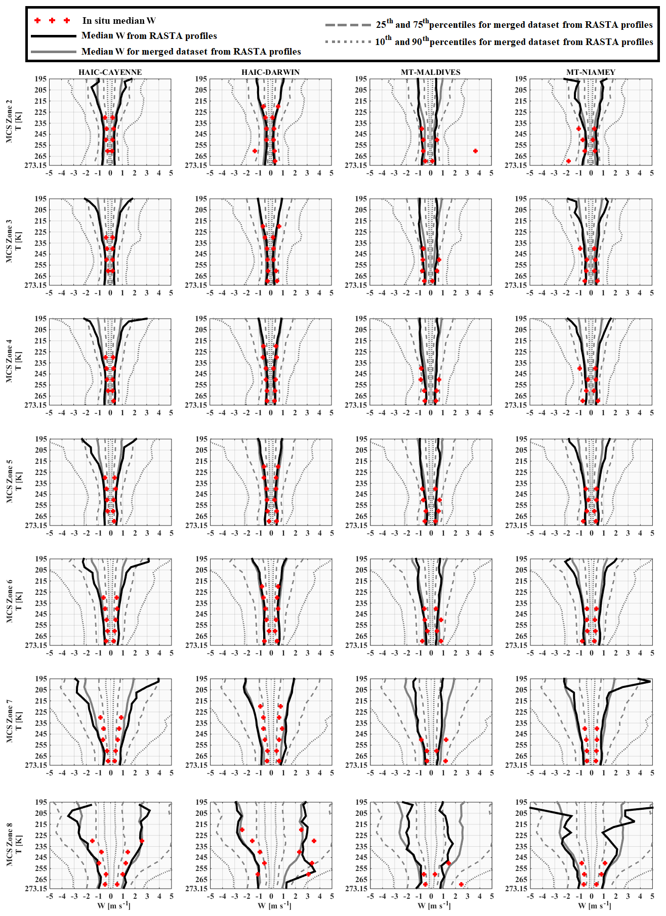
Figure 3 Vertical velocities for MCS reflectivity zone 2 to MCS reflectivity zone 8 from the top line to the bottom line, respectively.

In general, magnitude of updraft and downdraft increases with altitude and MCS reflectivity zones, where magnitudes of vertical velocity (negative and positive) are highest for MCS reflectivity zone 8. For all four datasets vertical wind speeds of MCS reflectivity zones 2–6 are smaller than or about 1 m s⁻¹.

To complete our investigation between MCS reflectivity zones and vertical velocity, we study the probability of observing vertical movement. We use a threshold for vertical velocity to distinguish between discernible and non-discernable vertical movement. We take a value of roughly 1 m s⁻¹ to be the threshold for detecting vertical movement (Houze 2004), i.e., at −1 m s⁻¹ < w < 1 m s⁻¹ there is no noticeable vertical movement upward or downward. The decision of taking a threshold of 1m s⁻¹ for updraft and downdraft is motivated by the fact that we have to take into account the measurement uncertainty (less than 0.25–0.5m s⁻¹). Additionally, we know that the variance of vertical turbulence is about 1.5 m² s⁻² (taken from large eddy simulations at 50 m resolution; Verrelle et al., 2017; Strauss et al., 2019). The fact that median w_ret for the merged dataset in MCS reflectivity zones 2 to 6 is smaller than 1 m s⁻¹ confirms our decision to use a threshold of 1 m s⁻¹.

Therefore, knowing T and Z, a probability to observe $\left|w_{\text{ret}}\right|\ge$ 1 m s⁻¹ is calculated as a function of MCS reflectivity zone and temperature, both for in situ measurement and cloud radar measurement. The solid colored lines in Fig. 4 are probabilities calculated from RASTA measurements, and the dashed lines with stars are probabilities calculated with vertical velocity measured at the aircraft level (in situ measurements). Both types of probabilities are different in each MCS zone and probabilities made with in situ measurements are smaller than those calculated with RASTA retrievals, except in MCS reflectivity zone 8 in Darwin where they are instead similar. Hence, in the point of view of observations of vertical velocity, statistics are different between in situ measurements and RASTA retrievals; i.e., there are different probabilities of observing vertical velocity with magnitudes larger than 1 m s⁻¹ (updraft and downdraft) for the same range of Z and range of T.

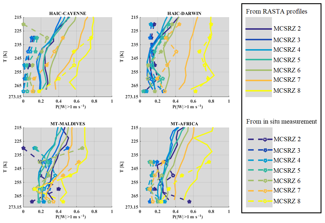
Figure 4 Probability to observe vertical velocity with an absolute magnitude larger than 1 m s⁻¹ in each MCS reflectivity zone (MCSRZ; color scale) for measurements from the radar Doppler RASTA (solid lines) and in situ measurements (dashed lines with stars).

In Fig. 4 we show that the probability of observing $\left|w_{\text{ret}}\right|\ge$ 1 m s⁻¹ is highest for MCS reflectivity zone 8 followed by zones 7 and 6, meaning that these MCS reflectivity zones tend to be more impacted by vertical movement (convective areas of MCS) than is the case for other MCS reflectivity zones. Additionally, these probabilities generally increase with altitude for all airborne campaigns, which matches the conclusions from Fig. 3. Generally, in MCS reflectivity zones 5, 4, 3, and 2, the probabilities $P\left(\right|w_{\text{ret}}\ge$ 1 m s⁻¹) as a function of T are close to each other, with a decreasing trend as reflectivity decreases, except for during the Maldives campaign. Statistically, MCS reflectivity zones 7 and 8 represent the most convective part of our observations in MCS for all four datasets. In contrast, MCS reflectivity zone 2 to 5 represent the stratiform part of MCS that has significantly lower vertical wind speeds.

4 Method of intercomparison

This study compares and discusses a series of ice cloud properties, such as IWC, visible extinction, the α and β coefficients of the dynamically retrieved m(D) power law, the size of the largest ice crystal of PSD, crystal number concentrations N_T, PSD second and third moments (M₂ and M₃, respectively), and the ratio of IWC∕M₂. The above-mentioned ice hydrometeor properties in all four MCS locations will be investigated as a function of T and MCS reflectivity zones (range of Z given by percentiles of Z as a function of T), which were both introduced in Sect. 3. In Sect. 5 a series of figures presenting results for the above-mentioned ice cloud properties (parameter X) will be presented in a uniform format. In all these figures (Figs. 5, 7, 9, 11, 13, 15, 17, 21, 23, 25) we show the median values of X by averaging MCS data from the four merged datasets (with the 25th and 75th percentiles represented by whiskers), as a function of T and MCS reflectivity zones (colored lines). The grey band shows the 25th and 75th percentiles of the parameter for the entire merged dataset, thereby merging data from all MCS reflectivity zones. The median and 25th and 75th percentiles of all parameters in each MCS reflectivity zone presented in the figures for the merged dataset are given in Appendix C in order to allow for comparisons with other datasets and evaluations of numerical weather predictions. If the range of variability of this median of parameter X in MCS reflectivity zone i, defined by its 25th and 75th percentiles, does not overlap with corresponding ranges of variability of X defined by the 25th and 75th percentiles of MCS reflectivity zones i−1 and i+1, respectively, we assume that this makes the median (four tropical campaigns) of X a candidate for X parametrization as a function of MCS reflectivity zone and T.

Thus, in Figs. 6, 8, 10, 12, 14, 16, 18, 22, 24, and 26 we calculate the median relative difference in percent (hereafter MRD-X) for all four individual MCS datasets – Cayenne (a), Darwin (b), the Maldives (c), and Niamey (d) – with respect to the median of X as a function of MCS reflectivity zone and T. In order to take into account the uncertainties in all types of measurements (hereafter referred to as U(X)∕X), uncertainties (represented by grey bands) for each parameter X were taken from Baumgardner et al. (2017).Thus, when the MRD-X is larger than U(X)∕X, it means that there is a significant difference between the median of the studied parameter for the merged dataset and the respective X of the selected individual MCS dataset. For cases where MRD-X is smaller than or equal to U(X)∕X, the median of X of the merged dataset, under the condition that the median (four tropical campaigns) of X is distinguishable between neighboring MCS reflectivity zones, can be used for the respective type of MCS. Hence, if the latter case is true for all four MCS locations, then the median (four tropical campaigns) of X is suitable to represent all four types (i.e., locations) of observed MCS.

Note that in all figures (Figs. 5–26) temperature of in situ observations is shown on the y axis and MCS reflectivity zones are color-coded.

The comparison of ice hydrometeor properties of the four MCS locations investigated in this study will mainly focus on the question of whether MRD-X (for individual MCS reflectivity zones) is larger or smaller than U(X)∕X depending on MCS location.

For each parameter presented in this study, either for the merged dataset or the campaigns individually (for calculation of MRD-X), the calculations are performed with the same conditions. The samples in each condition (T range and MCS reflectivity zones) are the same size for all parameters. Indeed, data are selected if they meet the temperature and radar reflectivity criteria, but the total concentration has to also be positive (for D_max> 50 µm), thus mixed-phase conditions are excluded. Therefore, the size of the samples is equal (i.e., number of data points in each ranges of T and of Z) for IWC, visible extinction, the α and β coefficients of m(D) power law, the largest particle of PSDs, crystal number concentrations NT, PSD second and third moments (M₂ and M₃, respectively), and the ratio of IWC∕M₂.

5 In situ observations in tropical MCS: the HAIC-HIWC and Megha-Tropiques projects

5.1 Ice water content

This section discusses the IWC measured during the HAIC-HIWC project and the IWC retrieved for the Megha-Tropiques project. IWC from the four datasets were merged to calculate the main statistic (merged dataset). Figure 5 shows median IWC for the merged dataset as a function of T and as a function of MCS reflectivity zones (color-coded lines). The graphical representation is limited solely to medians of IWC for MCS reflectivity zones 4 to 8 because IWC in MCS reflectivity zones 2 and 3 is linked to IWC smaller than 0.1 g m⁻³ where IWC data are subject to less confidence. In total, 30 % of the data observed in the four tropical datasets have an IWC lower than 0.1 g m⁻³ because the lower limit of MCS reflectivity zone 4 is defined with the 30th percentile of Z. The figure reveals that IWC increases with increasing MCS reflectivity zone for a given range of temperature. IWC median values clearly differ as a function of MCS reflectivity zone for the entire range of temperatures, with only a few exceptions above the freezing level (T∈ [265 K; 273 K[), i.e., between MCS reflectivity zones 4 and 5, and MCS reflectivity zones 7 and 8, with a small overlap in IWC ranges. In MCS reflectivity zones 4 to 7, median IWC increases with increasing T between 215 K and 260 K (where IWC has its maximum) and then slightly decreases as T further increases towards 273 K. In MCS reflectivity zone 8, IWC behaves rather similarly, with its maximum IWC already reached at 250 K.

Figure 5 The median of IWC in g m⁻³ given on the x axis, as a function of temperature in K on the y axis for different MCS reflectivity zones. Results for the merged dataset include both MT and HAIC-HIWC datasets. The grey band represents the 25th and 75th percentiles of the merged dataset. The extremities of the error bar show the 25th and 75th percentiles of IWC in each MCS-RZ. Lines are color coded as a function of the MCS reflectivity zones where in situ measurements were performed, and dashed color-coded lines represent the polynomial fit.

Figure 6 shows MRD-IWC for the four different campaigns. It is necessary that we recall that median IWC as a function of T and MCS reflectivity zone is calculated using a merged dataset where there are IWC from direct measurements and retrieved IWC from Z and PSD (Fontaine et al., 2017). Following this, there are two different uncertainties to consider to evaluate the MRD-IWC in each campaign. Firstly, for the Darwin and Cayenne campaigns the IWC were measured with an IKP-2 probe (direct measurement) with an uncertainty in measured IWC that increases with temperature (∼ 5 % at 220 K and ∼ 20 % at 273.15 K; Strapp et al., 2016a). Secondly, for the Niamey and the Maldives campaigns IWC were retrieved using the method described by Fontaine et al. (2017) (indirect measurement), with an uncertainty in regard to the IKP estimated by about ± 32 %. Hence, in Fig. 6a and b the grey bands show the uncertainty of the IKP-2 probe that was used for Cayenne and Darwin campaigns, while in Fig. 6c and d the grey bands describe the uncertainty in the retrieval method for IWC that was used for the datasets of Niamey and the Maldives.

Note that confidence in direct bulk IWC measurements from the IKP-2 is significantly higher than in indirect IWC calculations from the retrieval method (Fontaine et al., 2017).

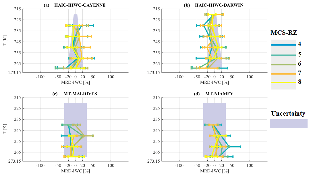
Figure 6 Median relative difference (MRD) of IWC during (a) HAIC-HIWC in Cayenne, (b) HAIC-HIWC in Darwin, (c) Megha-Tropiques in the Maldives, and (d) Megha-Tropiques in Niamey, with respect to the median of IWC for the merged dataset on the x axis as a function of temperature in K on y axis. The grey bands represent the uncertainties of the IWC measurement in (b) and (c) and the median deviation between the measurements and the IWC retrieval method (Fontaine et al., 2017) in (d) and (e). Lines are color coded as a function of the MCS reflectivity zones where in situ measurements were performed. The extremities of the error bar show the 25th and 75th percentiles of IWC relative error in each MCS reflectivity zone.

Therefore, Fig. 6a–d shows MRD-IWC for all MCS reflectivity zones as a function of T. For all four tropical MCS, MRD-IWC in MCS reflectivity zones 4 to 8 are distributed around 0 and are, in general, less than 30 %–40 % (25th to 75th percentiles). Measured IWC in MCS reflectivity zone 8 is in good agreement with the median IWC for all four tropical datasets. Uncertainty U(IWC)∕IWC for IKP-2 measurements (Darwin and Cayenne), especially at high altitude (about 5 %), is smaller than the expected deviation MRD-IWC. For middle and lower altitudes, MRD-IWC for Darwin and Cayenne, particularly for zones 5 and 8, is of the order of corresponding U(IWC)∕IWC. Concerning MCS over Niamey and the Maldives, MRD-IWC (25th to 75th percentiles) in general does not exceed corresponding U(IWC)∕IWC.

For comparison purposes with former studies, two IWC–T relationships from literature are added in Fig. 5. Jensen and Del Genio (2003) suggested an IWC–T relationship in order to account for the limited sensitivity of the precipitation radar aboard the TRMM satellite, which did not allow for small ice crystals at the top of convective clouds' anvils to be observed. They used radar reflectivity factors from a  35 GHz radar based on Manus Island (northeast of Australia; 2.058^∘ S, 147.425^∘ E), thereby calculating IWC from an IWC–Z relationship (IWC = 0.5 × (0.5.Z^0.36); Jensen et al., 2002). The resulting IWC–T relationship given by Jensen and Del Genio (2003) is reported by a dashed–dotted grey line, which fits between the 75th percentile of merged median IWC of MCS reflectivity zone 4 and the 25th percentile of MCS reflectivity zone 5. We recall that IWC, as a function of T, in MCS reflectivity zones 4 and 5 is related to Z between the 30th and 50th and 50th and 70th percentiles, respectively. Hence, the IWC–T relationship from Jensen and Del Genio (2003) is more adapted to stratiform parts of MCS where convective movement occurs less often.

Moreover, Heymsfield et al. (2009) established an IWC–T relationship based on seven field campaigns (black line in Fig. 5). They focused their study on maritime updrafts in tropical atmosphere for a temperature range T∈ [213.15 K; 253.15 K]. Their suggested IWC tends to be in the range of IWC of MCS reflectivity zones 6–8 with IWC increasing with T. We already showed in Sect. 3.2 that MCS reflectivity zones 7 and 8 have higher probabilities of being convective (updraft regions with higher magnitudes of vertical velocity), as compared to other MCS reflectivity zones. Therefore, the Heymsfield et al. (2009) IWC parameterizations for maritime updrafts are not inconsistent with data from this study.

Overall, this section demonstrates that variation in IWC with the temperature is similar in all types of MCS for corresponding ranges of radar reflectivity factors. Hence, we assume that IWC–Z–T relationships developed in Protat et al. (2016) are valid for all types of MCS in the tropics, at least for IWC larger than 0.1 g m⁻³.

5.2 Visible extinction

Figure 7 shows visible extinction coefficients (σ) calculated from OAP 2-D images (approximation of large particles; Van de Hulst, 1981), where S(D_max) is the projected area recorded by OAP and ΔD_max is the bin resolution equal to 10 µm:

$$\begin{array}{}\text{(1)}& \mathit{\sigma }=\mathrm{2}\cdot \sum _{\mathrm{15}\mathrm{\mu }\mathrm{m}}^{\mathrm{12845}\mathrm{\mu }\mathrm{m}}N\left(D_{\text{max}}\right)\cdot S\left(D_{\text{max}}\right)\cdot \mathrm{\Delta }{D}_{\text{max}}\left[{\mathrm{m}}^{-\mathrm{1}}\right],\end{array}$$

Figure 7 The same as Fig. 5 but for visible extinction σ given on x axis in m⁻¹.

In Fig. 7, median σ for the merged dataset (four tropical campaigns) increases with MCS reflectivity zone as expected and also increases with altitude (decrease with T), with larger gradients for T∈ [245; 273.15] than for T∈ [215 K; 245 K] in MCS reflectivity zones 5 to 8.

The uncertainty (U(σ)∕σ) (grey band in Fig. 8a–d) is calculated as follows:

$$\begin{array}{}\text{(2)}& {\displaystyle \frac{U\left(\mathit{\sigma }\right)}{\mathit{\sigma }}}=\sqrt{\mathrm{2}\cdot {{\displaystyle \frac{U\left(D\right)}{D}}}^{\mathrm{2}}+{{\displaystyle \frac{U\left(N\right)}{N}}}^{\mathrm{2}}},\end{array}$$

with $\frac{U\left(D\right)}{D}=\pm \mathrm{20}\mathit{\%}$, taking into account the uncertainty in the calculation of the size of hydrometeors and $\frac{U\left(N\right)}{N}=\pm \mathrm{50}\mathit{\%}$ for the uncertainty in the calculation of the concentration of hydrometeors from optical array probes (Baumgardner et al., 2017). The above uncertainties are those for particles larger than 100 µm. Note that if we took uncertainties for particles smaller than 100 µm (with ($U\left(D\right))/D=\pm$ 50 % and ($U\left(N\right))/N=\pm$ 100 %), the uncertainty in the calculation of σ would increase to ± 122 %. The reason why we do not take into account uncertainties of smaller particles is due to the fact that these particles contribute little to the visible extinction (2 % in the range [235 K; 273.15] and 10 % in the range [215 K; 225 K].

For all four types of tropical MCS, MRD-σ shown in Fig. 8a–d are in general smaller or equal to $\pm \frac{U\left(\mathit{\sigma }\right)}{\mathit{\sigma }}$. Hence, visible extinction in tropical MCS tends to be similar for all types of MCS observed in the same range of T and MCS reflectivity zone.

Figure 8 The same as Fig. 6 but for visible extinction MRD-σ.

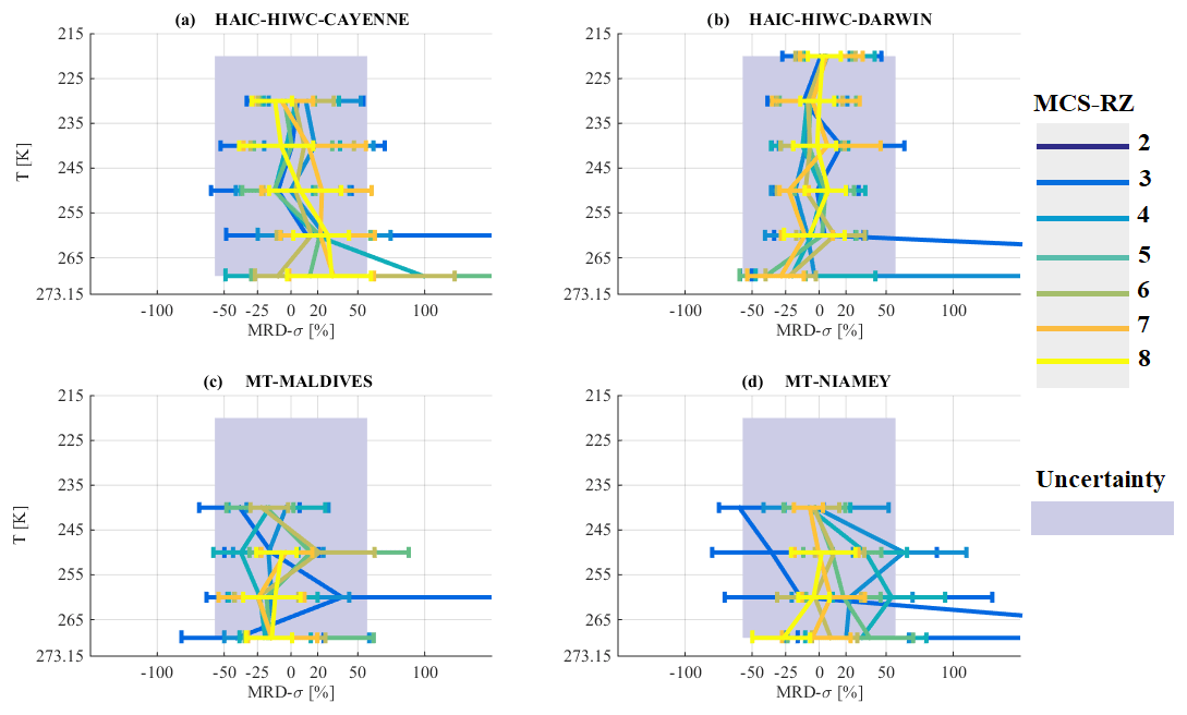
Furthermore, a σ–T relationship from Heymsfield et al. (2009) (black line) is added in Fig. 7, which is calculated, as a function of T, as the sum of the total area of particles larger than 50 µm plus the total area of particles smaller than 50 µm times a factor of 2, in order to satisfy Eq. (1) and to compare with the results of this study. We conclude that the σ−T estimation presented in Heymsfield et al. (2009) for maritime convective clouds is rather comparable to median σ calculations (merged dataset) in MCS reflectivity zones 6 to 7, corresponding to higher reflectivity zones and thus statistically to zones with some remaining convective strength.

5.3 Concentration of ice hydrometeors

Observed total concentrations for the merged datasets integrating particle sizes beyond 50 µm (N_T(D_max>50 µm); hereafter N_T,50) are presented as follows:

$$\begin{array}{ll}{\displaystyle }{N}_T(D_{\text{max}}>\mathrm{50}\mathrm{\mu }\mathrm{m})=& {\displaystyle }\sum _{D_{\text{max}}=\mathrm{50}}^{D\text{max}=\mathrm{12845}}N\left(D_{\text{max}}\right)\\ \text{(3)}& {\displaystyle }& {\displaystyle }\cdot \mathrm{\Delta }{D}_{\text{max}}\left[L^{-\mathrm{1}}\right].\end{array}$$

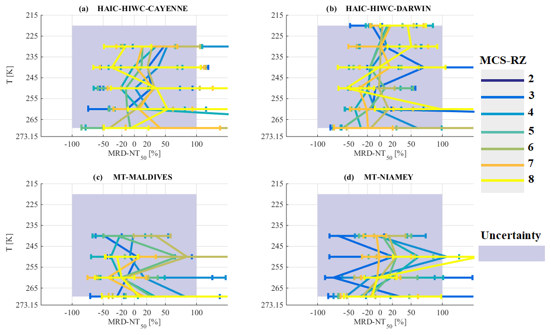
The median of N_T,50 as a function of T and MCS reflectivity zones is shown in Fig. 9, and MRD-N_T,50 for the four tropical MCS locations is shown in Fig. 10a–d. We observe an increase in median N_T,50 with altitude for all MCS reflectivity zones. N_T,50 also increases with MCS reflectivity zones for a given T, with the highest N_T,50 in MCS reflectivity zone 8. The range of variability for N_T,50 reveals significant overlap of the 25th and 75th percentiles of neighboring MCS reflectivity zones.

Figure 10 shows MRD-NT₅₀ where measurement uncertainty in concentrations are assumed ± 100 % (Baumgardner et al., 2017). MRD-N_T,50 in four different tropical MCS locations, particularly for higher MCS reflectivity zones, are of the order and even larger (75th percentile MRD-N_T,50) than the measurement uncertainty, even if the limit of concentrations of ice hydrometeors are not well defined between neighboring MCS reflectivity zones (Fig. 9). These concentrations tend to be similar for a given range of T and Z for the four different MCS locations.

A similar investigation is performed for total concentrations integrating beyond 15 µm (NT). Since the major conclusions are similar to those given for NT₅₀, data for N_T are shown in the figures in in Appendix A. Overall, the median of N_T,50 for the merged dataset is smaller by about an order of magnitude with respect to the median of N_T for the same MCS reflectivity zone. N_T over the Maldives tends to be larger than median N_T for the merged dataset. It shows that for a given range of T and Z, we can observe very different concentrations (by a factor of 10 even larger) of very small particles (about 15 to 50 µm) over the four different MCS locations (especially for the Maldives, i.e., oceanic MCS). However, when looking at total concentrations beyond 50 µm, the differences between the four locations mitigate each other, thus the four locations MRD-NT₅₀ are similar to or smaller than the measurement uncertainty of ice hydrometeor concentrations.

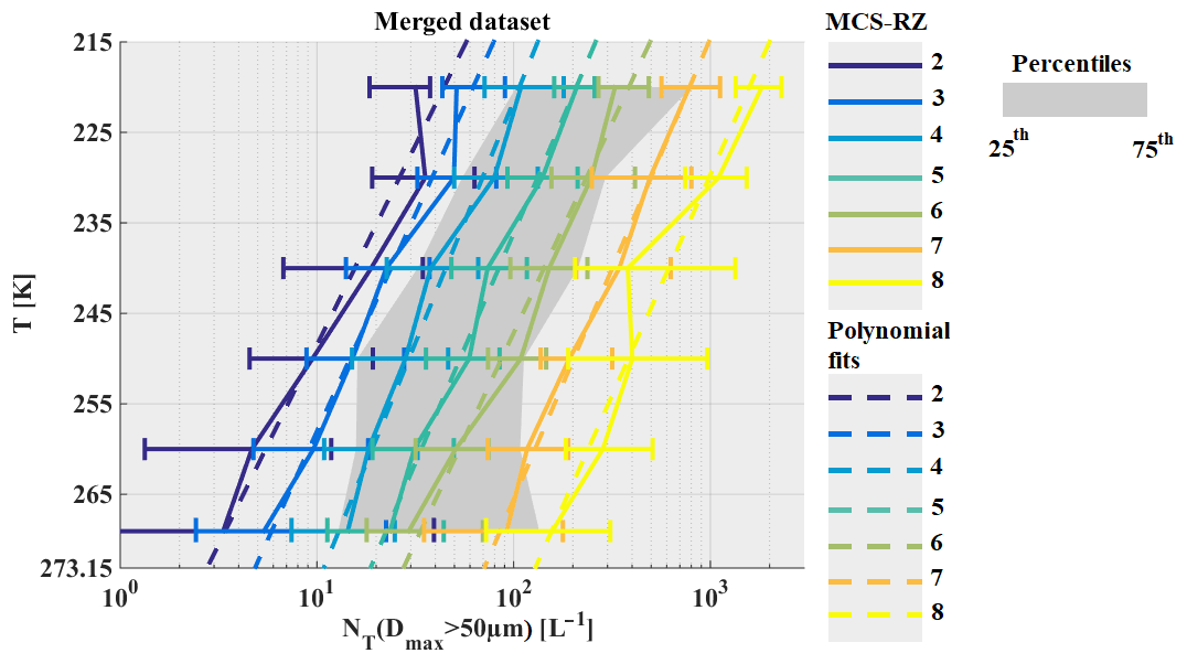
Figure 9 The same as Fig. 5 but for total concentrations integrated beyond D_max=50 µm in L⁻¹.

Figure 10 The same as Fig. 6 but for MRD-NT₅₀.

Concerning concentrations of larger hydrometeors, Fig. 11 shows concentrations of hydrometeors when PSD is integrated beyond 500 µm (hereafter, N_T,500; Eq. 4) and where the uncertainty in their measurement is estimated as being about ± 50 % for hydrometeors larger than 100 µm (Baumgardner et al., 2017).

$$\begin{array}{ll}{\displaystyle }{N}_T(D_{\text{max}}>\mathrm{500}\mathrm{\mu }\mathrm{m})=& {\displaystyle }\sum _{D_{\text{max}}=\mathrm{505}}^{D_{\text{max}}=\mathrm{12845}}N\left(D_{\text{max}}\right)\\ \text{(4)}& {\displaystyle }& {\displaystyle }\cdot \mathrm{\Delta }{D}_{\text{max}}\left[L^{-\mathrm{1}}\right].\end{array}$$

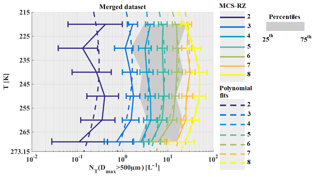
Figure 11 The same as Fig. 5 but for concentrations of hydrometeors integrated beyond D_max=500 µm in L⁻¹.

In Fig. 11, median N_T,500 is presented as a function of T and MCS reflectivity zone. The curves of median N_T,500 are different from curves of median N_T and N_T,50. Indeed, particularly for higher MCS reflectivity zones and in lower altitude levels (T∈ [250 K; 273.15 K]), N_T,500 tends to increase with altitude, reaches a maximum value around T∈ [235 K; 250 K], and then decreases for T∈ [215 K; 235 K]. The range of variability for N_T,500 reveals a rather small overlap, if any, of the 25th and 75th percentiles of neighboring MCS reflectivity zones 8, 7, and 6, mainly at coldest T∈ [215 K; 225 K]. There is no overlap for MCS reflectivity zones 2–5, and concentration of ice hydrometeors beyond 500 µm is instead constant from 215 to 265 K for observations in MCS reflectivity zones 3 to 5.

Figure 12 The same as Fig. 6 but for MRD-NT₅₀₀.

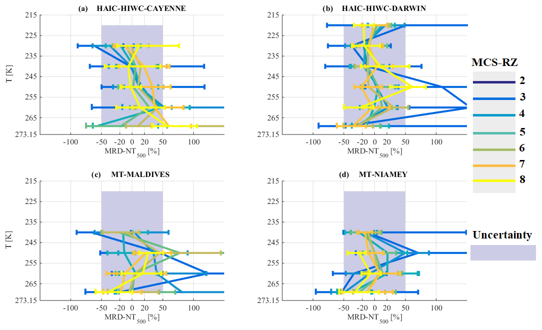
Figure 12a–d reveals that MRD-N_T,500 in higher MCS reflectivity zones is considerably smaller or roughly equal to the measurement uncertainty for large hydrometeors. Some smaller exceptions are noticeable where MRD-N_T,500 is larger than the measurement uncertainty for very low altitudes at T∈ [265 K; 273.15 K[, namely in Cayenne in MCS reflectivity zones 7 and 8 and Darwin in MCS reflectivity zone 8. Note that, in general, MRD-N_T,500 has smaller 75th percentiles (from Fig. 10b–e) compared to respective MRD-N_T,50 and MRD-N_T, showing that variability in each MCS reflectivity zone for hydrometeors larger than 500 µm is smaller than the variability of concentrations that include smaller (N_T,50) and the smallest (N_T) hydrometeors. This finding is clearly related to the uncertainty estimation given by Baumgardner et al., (2017) that small hydrometeors (D_max< 100 µm) have a larger estimated uncertainty of 100 % (due to shattering and very small sample volume), compared to the uncertainty of only 50 % for larger hydrometeors (D_max> 100 µm). Hence, it is not surprising that variability around a median value is larger for N_T and N_T,55 than for N_T,500. It is important to repeat here not only that MRD-N_T,500 is smaller than the uncertainty of 50 % but also that MRD-N_T,500 is tremendously smaller than MRD-N_T,50 and MRD-N_T. Despite this, we have to keep in mind that we will never have sufficient statistics from flight data, due to the sampling bias of flight trajectories and variability of microphysics from one system to another. Indeed, Leroy et al. (2017) demonstrated that median mass diameter MMD_eq generally decreases with T and increasing IWC for the dataset of HAIC-HIWC over Darwin. However, for two flights performed in the same MCS, Leroy et al. (2017) showed that high IWC were linked to large MMD_eq, where MMD_eq tends to increase with IWC. This demonstrates that comparable high IWC can be observed for two different microphysical conditions (short-lived typical oceanic MCS versus long-lasting tropical storms in the same dataset).

We observe that total concentrations starting from 15 µm can be different between MCS locations as a function of T and Z, especially in oceanic MCS over the Maldives in the more stratiform part of the MCS, where measured concentrations can reach 10 times the median concentrations observed for the merged dataset. MCS over Niamey also show larger concentrations near the convective part of the MCS. However, concentrations of ice hydrometeors beyond 50 µm tend to be more similar as a function of T and Z for all type of MCS, even if the limits between each MCS reflectivity zone are not well defined.

Between the four MCS locations, differences of aerosol loads and available ice nuclei might exist. Despite these possible differences, ice crystal formation mechanisms may be primarily controlled by dynamics, thermodynamics, and (particularly) secondary ice production rather than the primary nucleation (Field et al., 2016; Phillips et al., 2018; Yano and Phillips, 2011) that regulates the concentrations of hydrometeors beyond ∼ 55 µm, making these concentrations rather similar for different MCS locations.

5.4 Coefficients of mass–size relationship

The relationship between mass and size of ice crystals is complex. Usually in field experiments the mass of individual crystals is not measured, instead bulk IWC is measured, which is the integrated mass of an ice crystal population per sample volume linked to PSDs of ice hydrometeors. However, IWC is not always measured or is measured with low accuracy. Due to the complex shape of ice hydrometeors, various assumptions allow us to estimate the mass of ice crystals for a given size. Indeed, many habits of ice crystals can be observed in clouds, primarily as a function of temperature and ice saturation (Magono and Lee, 1966; Pruppacher et al., 1998). Hydrometeors of different habits can also be observed at the same time (Bailey and Hallett, 2009). Locatelli and Hobbs (1974) and Mitchell (1996) suggested mass–size relationships represented as power laws with $m=\mathit{\alpha }\cdot D^{\mathit{\beta }}$ for different precipitating crystal habits. Coefficients α and β vary as a function of ice crystal habit. Further studies performed calculations of mean mass–size relationships (also using power law approximations) retrieved from simultaneous measurements of particle images combined with bulk ice water content measurements (Brown and Francis, 1995; Cotton et al., 2013; Heymsfield et al., 2010). Schmitt and Heymsfield (2010), Fontaine et al. (2014), and Leroy et al. (2016) showed that mass–size relationship coefficients α and β vary as a function of temperature. In the latter studies, coefficient β is calculated from OAP images and then α is retrieved either from processed images or constrained with integral measured IWC or radar reflectivity factor Z. Recently, Coutris et al (2017) retrieved masses of hydrometeors by an inverse method using direct measurement of PSD and IWC. In this latter study, the mass of ice crystals is retrieved without any assumption on the type of function linking mass and size of ice hydrometeors.

This study uses the power law assumption to constrain the mass of ice hydrometeors. Thereby, the β exponent of the mass–size power law relationship is calculated (Eq. 5) as presented in Leroy et al., (2016) for hydrometeors defined by D_max dimension:

$$\begin{array}{}\text{(5)}& \mathit{\beta }=\mathrm{1.71}\cdot f_{\mathrm{s}}-\mathrm{0.62}\cdot f_{\mathrm{p}}.\end{array}$$

Here, f_p is the exponent and e_p is the pre-factor of the perimeter–size power law relationship (Duroure et al., 1994) with $P\left(D_{\text{max}}\right)=e_{\mathrm{p}}\cdot D_{\text{max}}^{f_{\mathrm{p}}}$, in cm, while f_s is the exponent and e_s is the pre-factor of the 2-D image area–size relationship (Mitchell, 1996) with $S\left(D_{\text{max}}\right)=e_{\mathrm{s}}\cdot D_{\text{max}}^{f_{\mathrm{s}}}$, in cm². These two relationships are calculated using images from 2D-S and PIP. Hence, β is a proxy parameter that describes the global (all over the size range of hydrometeors from 50 µm to 1.2 cm) variability of the shape of the recorded hydrometeors during the sampling process (Leroy et al., 2016; Fontaine et al., 2014). Figure 13 shows the variability of β as a function of temperature and MCS reflectivity zone for the merged dataset. For a given MCS reflectivity zone, β increases with increasing temperature. For a given temperature, β also increases with MCS reflectivity zone, although MCS reflectivity zones 4, 5, 6, 7, and 8 share a range of common values for β, making it more uncertain to predict with a good accuracy using a parametrization as a function of IWC and T.

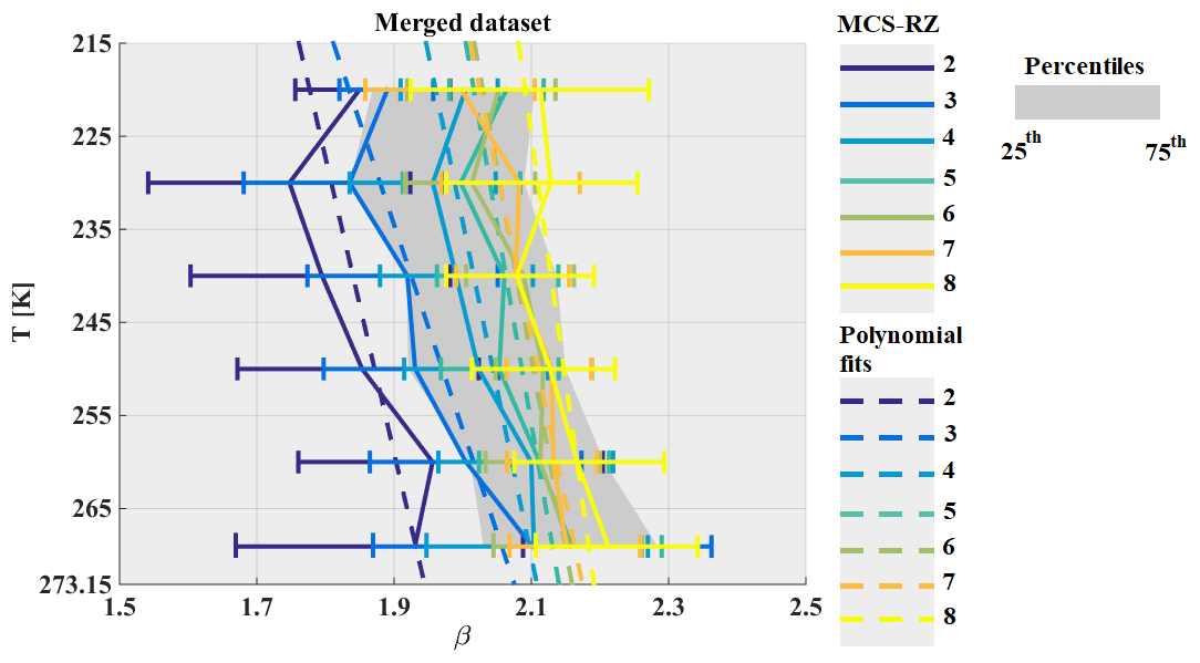
Figure 13 The same as Fig. 5 but for exponent β of mass–size relationships for the used ice hydrometeor size definition D_max.

In order to estimate the uncertainty in the calculation of β (grey band in Fig. 14a–d), results from Leroy et al. (2016) have been used, with $U\left(\mathit{\beta }\right)/\mathit{\beta }=\pm$ 2.3 %. However, if we had calculated the uncertainty in retrieved β from the uncertainty in the measurement of the size and concentration of hydrometeors from OAP images, the uncertainty would have been by about 44 %. Considering the small range of variability for β (1 to 3), the uncertainty given by Leroy et al. (2016) allows us to highlight some differences in overall ice particle habit. In general, MRD-β in MCS reflectivity zones 8 and 7 tends to be in the range of U(β)∕β, assuming that β are similar for all observed MCS in the four campaigns for the conditions described by MCS reflectivity zones 7 and 8.

Figure 14 The same as Fig. 6 but for the exponent of mass–size relationship MRD-β.

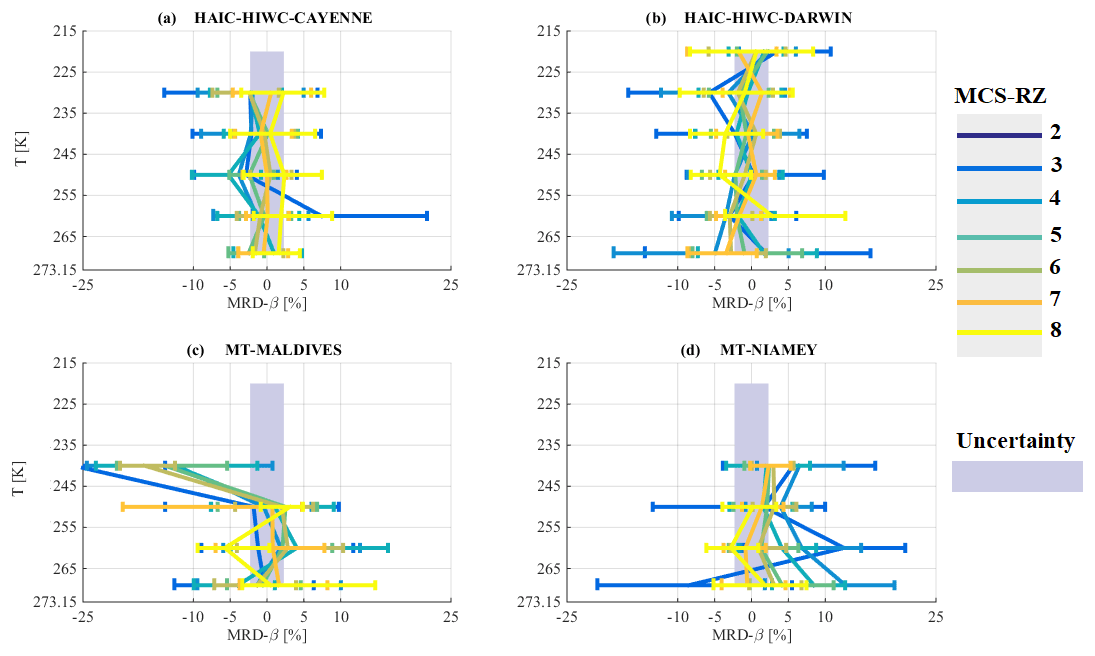
However, in MCS reflectivity zones 2 to 6 MRD-β is more scattered around U(β)∕β with occasionally larger MRD-β than uncertainty of β, especially for MCS over the Maldives and Niamey. Over the Maldives, at higher altitudes β tends to be smaller compared to the median β calculated for the merged dataset, while MCS over Niamey tends to have β larger than median β calculated for the merged dataset.

Overall, the predictability of β coefficients as a function of T and MCS reflectivity zone remains challenging. We are aware of the fact that the power law approximation has certain limits when trying to impose one single β to an entire crystal population composed of smaller (dominated by pristine ice) and larger crystals (more aggregation, also riming).

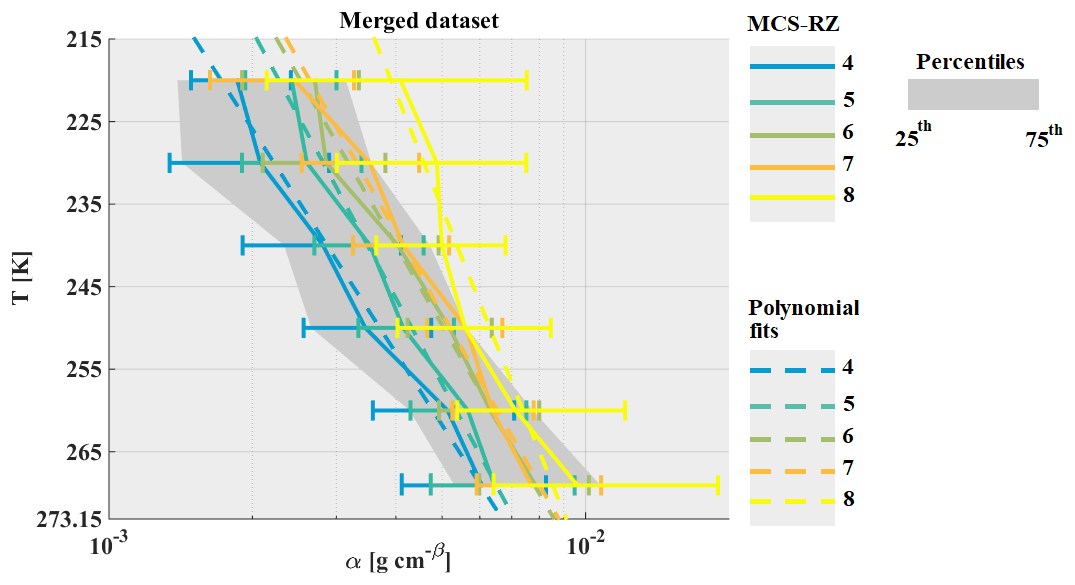
Figure 15 The same as Fig. 5 but for α of mass–size relationships for the used ice hydrometeor size definition D_max.

For HAIC-HIWC datasets, coefficient α is retrieved while matching measured IWC from IKP-2 with calculated IWC, thereby integrating the PSD times m(D) power law relationship. For the Maldives and Niamey datasets, coefficient α is retrieved from T-matrix simulations of the radar reflectivity factor (Fontaine et al., 2017).

For both situations, α calculation is solely constrained by the fact that the mass of ice crystals remains smaller than or equal to the mass of an ice sphere with the same diameter D_max:

$$\begin{array}{ll}{\displaystyle }\mathit{\alpha }=& {\displaystyle \frac{\text{IWC}}{{\sum }_{\mathrm{15}}^{\mathrm{12845}}N\left(D_{\text{max}}\right)\cdot D_{\text{max}}^{\mathit{\beta }}\cdot \mathrm{\Delta }{D}_{\text{max}}}}\mathrm{|}\\ \text{(6)}& {\displaystyle }& {\displaystyle }\mathit{\alpha }\cdot D_{\text{max}}^{\mathit{\beta }}\le \mathrm{0.917}\cdot {\displaystyle \frac{\mathit{\pi }}{\mathrm{6}}}\cdot D_{\text{max}}^{\mathrm{3}}\left[\mathrm{g}{\mathrm{cm}}^{-\mathit{\beta }}\right].\end{array}$$

For the uncertainty calculation of α, we take the maximum value of β of 3:

$$\begin{array}{}\text{(7)}& {\displaystyle \frac{U\left(\mathit{\alpha }\right)}{\mathit{\alpha }}}=\sqrt{{\left({\displaystyle \frac{U\left(\text{IWC}\right)}{\text{IWC}}}\right)}^{\mathrm{2}}+\mathrm{3}\cdot {\left({\displaystyle \frac{U\left(D\right)}{D}}\right)}^{\mathrm{2}}{\left({\displaystyle \frac{U\left(N\right)}{N}}\right)}^{\mathrm{2}}}.\end{array}$$

Figure 15 shows median α coefficients as a function of T and MCS reflectivity zone. As has been already stated in previous studies, α is strongly linked to the variability of β (Fontaine et al., 2014; Heymsfield et al., 2010). Figure 15, when compared to Fig. 13, confirms that results for α have similar trends to those discussed for β. However, α varies from 5.10⁻⁴ (in MCS reflectivity zone 2) to ≈ 2.10⁻² (in MCS reflectivity zone 8). In general, α increases as a function of T for a given MCS reflectivity zone and also increases as a function of MCS reflectivity zone (and associated IWC) for a given T level. As already stated for the median exponent β in Fig. 13, median α in MCS reflectivity zones 4, 5, 6, 7, and 8 is more or less overlapped.

Figure 16 The same as Fig. 6 but for the pre-factor of mass–size relationship MRD-α.

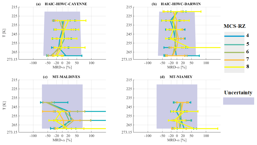
From Fig. 16a and b, we note that even with a good accuracy of measured IWC (from IKP-2; $U\left(\text{IWC}\right)/\text{IWC}\approx \pm$ 5 % for the typical IWC values observed in HAIC-HIWC at 210 K), the uncertainty of α is rather large, which is mainly due to uncertainties in OAP size and concentration measurements. Taking into account the large uncertainty in the retrieved α, we find that MRD-α for all four merged datasets for MCS reflectivity zones 4, 5, 6, 7, and 8 is smaller than U(α)∕α. For observations from Niamey (Fig. 16 (d)), α tends to be larger than median α for the merged dataset (MRD-α not centered on 0 but shifted to positive values).

In previous sections, this study documented similar IWC values and visible extinction coefficients for a given range of Z and T and a clear increase in IWC and visible extinction coefficient from MCS reflectivity zones 4 to 8. The increase in α and β with MCS reflectivity zones is not as clearly visible, whereas α at least seems to increase with temperature in different MCS reflectivity zones. Moreover, we cannot ignore that α and β tend to be larger in MCS reflectivity zone 8 than in MCS reflectivity zone 4, especially at higher altitudes. However, the increase in IWC and visible extinction with MCS reflectivity zone Z is not linked to an increase in the mass–size coefficients. This conclusion takes into account the variability of the mass–size coefficients shown by the 25th and 75th percentiles. Furthermore, ice hydrometeor habits described with β in MCS reflectivity zone 4, 5, and 6 are different in MCS over the Maldives and MCS over Niamey compared to MCS over Darwin and Cayenne (smaller β over the Maldives and larger β over Niamey).

As visible extinction (hence projected surface) and IWC are similar for the same range of T and Z in all types of MCS, but the shapes of crystals might be different from one to another MCS location, we assume that the ratio of projected surface versus IWC is similar. In other words, the density of ice per surface unity (or by pixels of projected surface) is similar as a function of T and Z in all types of MCS even if there might be a possibility that the habit or the shape could be different (pure oceanic MCS versus pure continental MCS). Note that these assumptions are established for IWC larger than 0.1 g m⁻³.

5.5 The largest ice hydrometeors

Figure 17 investigates the variability of the size of the largest ice hydrometeors in the PSD, hereafter referred to as max(D_max), as defined in Fontaine et al (2017). Figure 17 reveals that the median of max(D_max) increases with T for all MCS reflectivity zones, with larger hydrometeors at the cloud base compared to cloud top, particularly in the stratiform cloud part, where PSD are mainly impacted by a combination of aggregation and sedimentation. At higher levels for T∈ [215 K; 245 K[ the largest median of max(D_max) is observed in the most convective MCS reflectivity zone 8, followed by zones 7, 6, and 5, where sedimentation becomes more and more active. Below the 250 K level, the largest max(D_max) can be observed in MCS reflectivity zones 6 and 7 (still containing a significant sedimentation source from above), followed by 5 (increasing depletion of large crystals), and 8 (more convective or at least a transition zone from convective to stratiform cloud). The smallest max(D_max) are observed in MCS reflectivity zones 2 and 3.

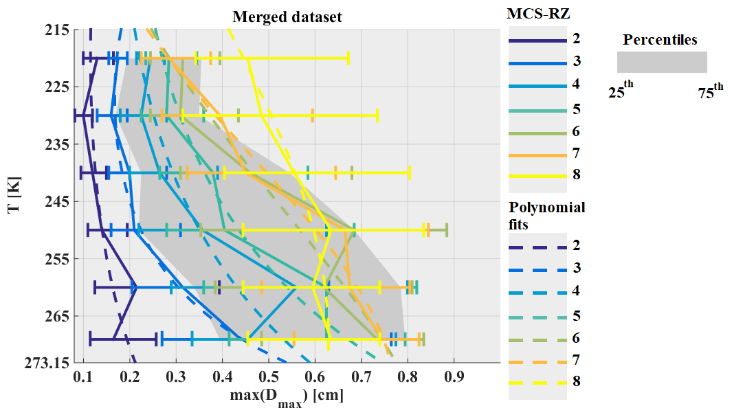
Figure 17 The same as Fig. 5 but for the maximum size of hydrometeors max(D_max) in PSD in cm.

MRD-max(D_max) shown in Fig. 18a–d is a bit larger than the measurement uncertainty estimated with ± 20 % (Baumgardner et al., 2017). Cayenne, Darwin, and Niamey data are centered around the median max(D_max) of the merged dataset in MCS reflectivity zone 8 for all types of MCS and in MCS reflectivity zone 7 for MCS over Darwin, Cayenne, and Niamey. MCS over Cayenne and Darwin tend to have similar max(D_max) in other MCS reflectivity zones. The Maldives dataset shows mainly negative MRD-max(D_max) values, indicating that max(D_max) for the Maldives data is generally smaller than that of the other three tropical locations. MCS over Niamey also show larger max(D_max) in MCS reflectivity zones 2 to 4, illustrating that snow aggregates can reach larger sizes during the West African Monsoon than in other MCS locations. This confirms the conclusions of Frey et al. (2011) and Cetrone and Houze (2009), who suggested that there are larger ice hydrometeors in MCS over continental regions than MCS over maritime regions.

Figure 18 The same as Fig. 6 but for maximum size of hydrometeors max(D_max).

In this section, it is shown that in the stratiform part of MCS, the largest hydrometeors are larger in MCS over Niamey than in other types of MCS and tend to be smaller in MCS over the Maldives. Large crystals (D_max>1 mm) are mainly agglomerates of pristine ice crystals, for which the growth process is led by aggregations (by sedimentation) instead of vapor diffusion. There is a possibility that the largest hydrometeors are large pristine ice. Indeed, some large pristine ice (large dendrites) was found in the dataset (especially over the Maldives; see Fig. 1 in Fontaine et al., 2014). However, their size does not exceed 3 to 4 mm. Hence, aggregation efficiency is different from one MCS type to another, and this could explain the differences of mass–size coefficient β, as it is calculated using the slope in a log–log scale of mean perimeter and mean surface as a function of median diameter in each size bin where large hydrometeors have a non-negligible impact on the slope (i.e., f_p and f_s; see Eq. 5).

5.6 Note on the impact of vertical velocity on ice microphysics

This section discusses the results of an investigation performed into the impact of vertical velocity on ice microphysical parameters presented earlier in Sect. 5. In addition to the statistics taken from the merged dataset where vertical velocity was not considered, similar statistics were calculated for three sub-datasets: (i) $w<-\mathrm{1}\mathrm{m}{\mathrm{s}}^{-\mathrm{1}}$, (ii) $-\mathrm{1}\mathrm{m}{\mathrm{s}}^{-\mathrm{1}}<w<\mathrm{1}\mathrm{m}{\mathrm{s}}^{-\mathrm{1}}$, and (iii) $w>\mathrm{1}\mathrm{m}{\mathrm{s}}^{-\mathrm{1}}$. Following this, median relative difference for the three conditions and for each parameter presented in this Sect. 5 was calculated and compared to the median relative difference when no distinction is performed as a function of vertical velocity. Firstly, we noticed that MRD-X for the merged dataset and MRD-X for the second condition (i.e., $\mathrm{1}\mathrm{m}{\mathrm{s}}^{-\mathrm{1}}<w<\mathrm{1}\mathrm{m}{\mathrm{s}}^{-\mathrm{1}}$) are similar (MRD-X, with X being used to replace IWC, σ, NT, NT₅₀, NT₅₀₀, β, α, and max(D_max)). Secondly, differences of MRD-X in updraft and downdraft in regard to MRD-X for the merged dataset and no vertical movement are all visible. However, most of the time these differences are of the order of or smaller than measurement uncertainties (U(X)∕X). Hence, the impact of vertical velocity (> 0 m s⁻¹ or < 0 m s⁻¹) on the ice microphysics parameters presented in Sect. 5 is not significant, except for IWC, NT, and NT₅₀. Figures for these three parameters are presented in Appendix B.

Appendix B shows when updraft has an impact on IWC N_T and N_T,50 for a given range of temperature and MCS reflectivity zones. Figure B1 shows MRD-IWC, Fig. B2 shows MRD-N_T, and Fig. B3 shows MRD-N_T,50. For the others parameters an impact related to updraft is uncommon.

It appears that updraft tends to mainly impact concentrations of small hydrometeors and IWC for some types of MCS and some MCS reflectivity zones. Thus, for N_T (Fig. B2), we observe larger N_T for updraft in MCS observed over Cayenne, the Maldives, and Niamey. For Cayenne, we come to a similar conclusion in MCS reflectivity zone 5 and 6 for temperatures between 245 K and 265 K, with N_T 2 to 3 times larger than N_T for merged dataset. For MCS over the Maldives, median N_T are 5 times to 20 times larger than N_T when there is no noticeable vertical movement in MCS reflectivity zones 6, 7, and 8. Finally, for MCS over Niamey, we observe larger N_T in updraft than N_T for the merged dataset in MCS reflectivity zones 6 for T around 240 K and in MCS reflectivity zones 8 above the bright band. We have similar conclusions for N_T,50 (Fig. B3), except that ratios between N_T,50 in updraft and N_T,50 when no updraft is present are smaller than the ratio between N_T in updraft and N_T when there is no updraft.

IWC are only impacted by updraft for MCS over Cayenne in MCS reflectivity zone 4, 5, 6, and 7. IWC in updraft tends to be larger by about +50 % than IWC when there is no updraft, except in MCS reflectivity zone 5, where IWC is about 2 times larger in updraft than IWC when there is no updraft.

This investigation into the impact of updraft and downdraft on ice microphysics shows that updraft may have an impact on concentrations of small hydrometeors and IWC. However, updraft does not impact all types of MCS in the same way. Therefore, there will need to be deeper investigations into updraft impact in the future.

Despite some noticeable impact of updraft on ice microphysics in our datasets, there are no significant (recurrent through all types of MCS or as a function of T or Z) results to assess them for the merged dataset. Thus, parameterizations developed in the next section are only as a function of IWC and T, with no consideration of convective movement.

6 Parameterizations as a function of IWC and T

6.1 Visible extinction

We conclude from Figs. 5 to 8 that visible extinction σ and IWC in tropical MCS tend to be similar for all MCS locations in the same range of T and for corresponding MCS reflectivity zones 4 to 8. Following from this, Figure 19 shows that there is a linear relationship between log(σ) and log(IWC), and that log(σ) decreases, with temperature increasing at constant log(IWC). We performed a surface fitting using input coefficients log(IWC) and T to fit log(σ) to deduce a parametrization of σ (Eq. 8) as a function of IWC and T. This parameterization is limited for deep convective cloud (merged dataset) and data using IWC > 0.1 g m⁻³:

$$\begin{array}{ll}{\displaystyle }\mathit{\sigma }=& {\displaystyle }\exp (-\mathrm{0.0194587}\cdot T+\mathrm{0.9134019}\cdot \text{ln}(\text{IWC})\\ \text{(8)}& {\displaystyle }& {\displaystyle }+\mathrm{1.2423609}\left)\right[{\mathrm{m}}^{-\mathrm{1}}].\end{array}$$

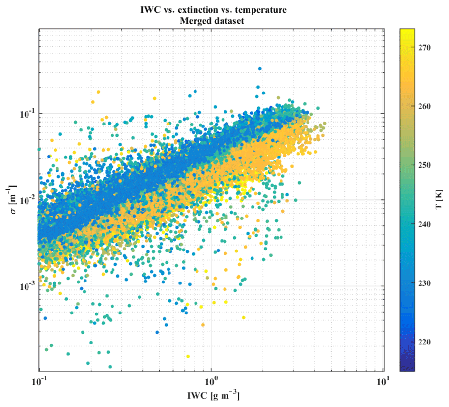
Figure 19 Visible extinction in m⁻¹ on the y axis as a function of IWC in kg m⁻³ on the x axis and as a function of T in K indicated by the color scale. Scatter plot using the merged dataset (four campaigns).

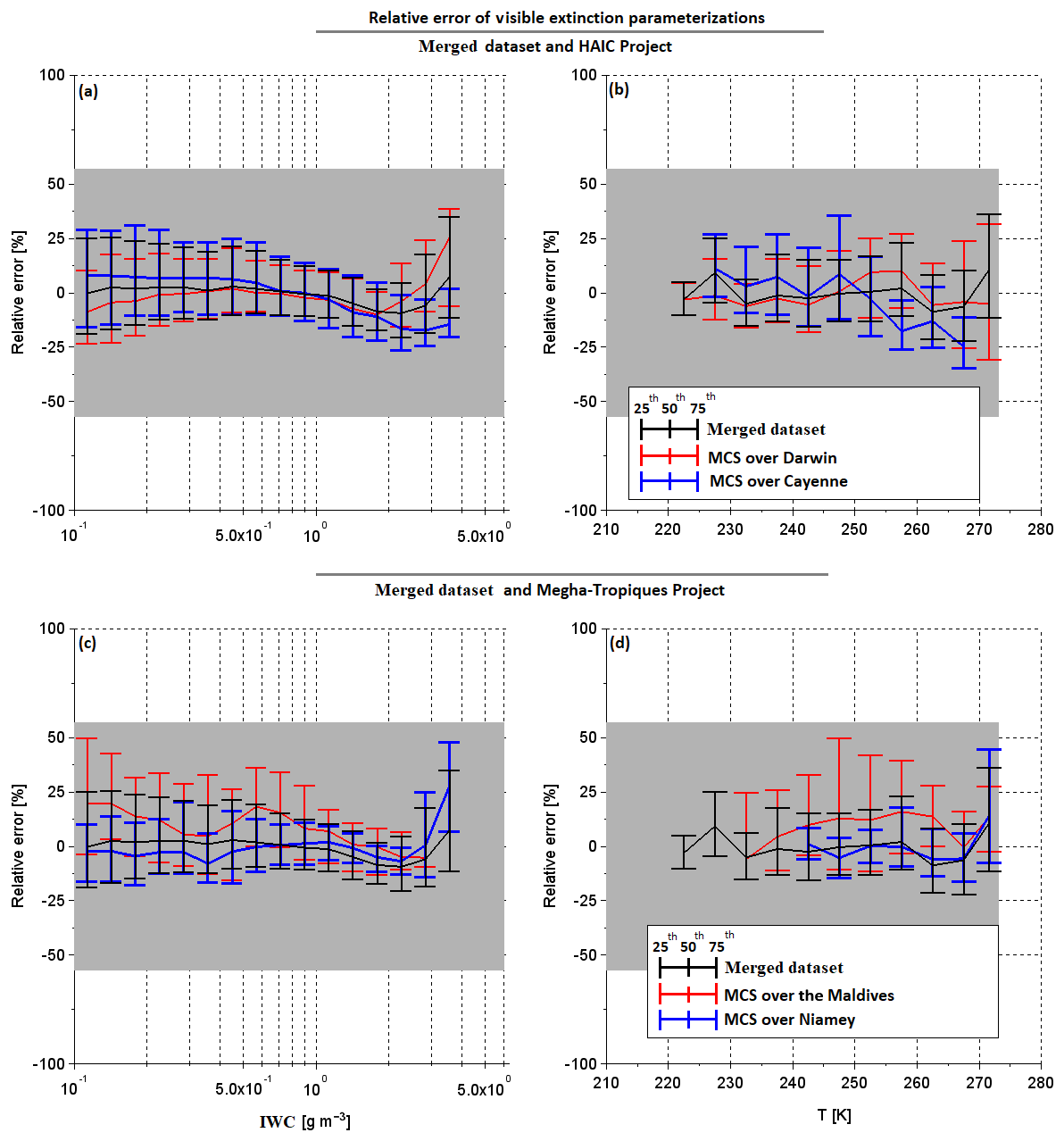
Figure 20 Relative errors of predicted visible extinction, Eq. (8), with respect to measured visible extinction for (a–d). Relative errors as a function of IWC in (a) and (c) and as a function of T in (b) and (d). The black lines in the four panels represent the relative errors when calculated for the merged dataset. In (a) and (b), the red lines show the median relative error for MCS over Darwin and the blue line shows the same for MCS over Cayenne. In (c) and (d), the red line represents the median relative error for MCS over the Maldives and the blue lines show the same for MCS over Niamey. The bottom of the error bar shows the 25th percentile of relative error, and the 75th percentile are given by the top of the error bar.

An evaluation of this parametrization is presented in Fig. 20, where black lines in Fig. 20a–d represent median relative errors of σ (with the 25th and 75th percentiles represented by whiskers) for the merged dataset predicted with Eq. (8) with respect to retrieved σ from OAP images from Eq. (1). In addition, median relative errors of σ for individual MCS datasets over Darwin, Cayenne, the Maldives, and Niamey with respect to σ calculations (Eq. 8) are shown in Fig. 20a–d, respectively. The uncertainty $\pm \frac{U\left(\mathit{\sigma }\right)}{\mathit{\sigma }}$ is given by the grey band. All relative errors (25th–75th percentile) tend to be smaller than $\pm \frac{U\left(\mathit{\sigma }\right)}{\mathit{\sigma }}$, with median relative errors that are smaller than ± 25 % of σ uncertainty calculated from Eq. (2). In general, Eq. (8) seems to produce the smallest relative errors for σ from the Niamey and Darwin datasets (especially for IWC < 2 g m⁻³).

It is worth noting that optically thick clouds are responsible for large errors in retrieved cloud water path and condensed water concentration profiles retrieved from satellite imagery (Smith, 2014; Yost et al., 2010). Parameterizations, such as presented here, could help to improve retrieval methods on cloud water path but more investigations on the benefits of such parameterizations are needed, which is beyond the scope of this study.

6.2 Parameterization of ice hydrometeor distributions

6.2.1 Observations of PSD moment

Moments of PSD are convenient for numerical weather prediction to model microphysics of hydrometeor populations, since knowing the PSD nth-order moment allows us to roughly describe cloud processes and their hydrometeors properties. Commonly, PSD of ice hydrometeors are modeled with gamma distributions (Heymsfield et al., 2013; McFarquhar et al., 2007). The calculation of the nth-order moment is defined in Eq. (9) for PSD obtained from measurements of hydrometeors images, e.g., with OAP as follows:

$$\begin{array}{}\text{(9)}& M_n=\sum _{D_{\text{max}}=\mathrm{50}\mathrm{\mu }\mathrm{m}}^{D_{\text{max}}=\mathrm{1},\mathrm{2}\mathrm{cm}}N\left(D_{\text{max}}\right)\cdot D_{\text{max}}^n\cdot \mathrm{\Delta }{D}_{\text{max}}\left[{\mathrm{m}}^{\mathrm{n}-\mathrm{3}}\right].\end{array}$$

The uncertainty of the nth moment (n=2 and 3 in our study) is as follows:

$$\begin{array}{}\text{(10)}& {\displaystyle \frac{U\left(M_n\right)}{M_n}}=\sqrt{n\cdot {{\displaystyle \frac{U\left(D\right)}{D}}}^{\mathrm{2}}+{{\displaystyle \frac{U\left(N\right)}{N}}}^{\mathrm{2}}}.\end{array}$$

.

Figure 21 The same as Fig. 5 but for M₂ m⁻¹

Figure 21 shows median second-moment M₂ as a function of T for all MCS reflectivity zones for the merged dataset. Median M₂ slightly decrease with temperature for all individual MCS reflectivity zones and distinctly increases with MCS reflectivity zone for a given T. The range of variability of median M₂ shows mainly negligible overlap, if any, of the 25th and 75th percentiles of neighboring MCS reflectivity zones, with the exception of between MCS reflectivity zones 8 and 7 at low altitude (T∈ [265; 273.15[).

Figure 22 The same as Fig. 6 but for MRD-M₂.

All four tropical MCS (Fig. 22a–d) show good agreement with the median of M₂ in MCS reflectivity zones 3 to 8, with MRD-M₂ being significantly smaller than U(M₂)∕M₂. A few minor exceptions can be found for MCS over Cayenne (Fig. 22b) and Darwin (Fig. 22c) in the temperature range [265 K; 273.15[. MCS over Niamey (Fig. 22e) also show a larger MRD-M₂ in MCS reflectivity zones 2 and 3 for T∈ [265 K; 273.15 K[ and T∈ [245 K; 255 K[, respectively.

Figure 23 The same as Fig. 5 but for the M₃ for the unity dimension.

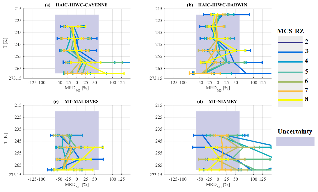
Figure 23 presents median third-moment M₃ for merged dataset as a function of T and for different MCS reflectivity zones. Median M₃ in highest MCS reflectivity zones 8, 7, and (to some extent) 6 resemble the corresponding curves of median IWC (Fig. 5), with a maximum value for median M₃ for T∈ [245 K; 260 K[. We also note an increase in median M₃ with MCS reflectivity zone from 2 to 8. The range of variability for M₃ reveals no overlap of the 25th and 75th percentiles of neighboring MCS reflectivity zones 2–7; only zone 7 overlaps with zone 8 for all temperatures. The third moment of MCS over Cayenne, Darwin, and the Maldives in MCS reflectivity zones 2 to 8 shows MRD-M₃ smaller than U(M₃)∕M₃, with a few minor exceptions in the range of T∈ [265 K; 273.15 K[. MCS over Niamey tend to have MRD-M₃ that are sometimes larger than U(M₃)/ M₃. Indeed, M₃ for MCS over Niamey tend to be larger in MCS reflectivity zones 5 and 2 in the range of T∈ [265 K; 273.15 K[, in MCS reflectivity zone 4 for T larger than 255 K, and in MCS reflectivity zone 3 for T larger than 245 K.

Figure 24 The same as Fig. 6 but for the M₃.

Overall, this section illustrates that the second and third moments of PSD are similar as a function of T and Z for all MCS locations of the underlying dataset. However, there are exceptions in MCS reflectivity zones 2, 3, and 4 in MCS over Niamey where larger third moments are calculated compared to those deduced for the merged dataset. Despite those exceptions, the next section explores the possibility to parameterize the second and third PSD moments as a function of IWC and temperature.

6.2.2 Parameterizations of M₂ and M₃

This section presents parameterizations to predict the second and third moment of the PSD for the merged dataset as a function of T and IWC (for this section IWC is given in kg m⁻³), including IWC data larger than 0.1 g m⁻³. Indeed some moments can be directly linked to bulk properties of hydrometeor populations. For example, moment M₀ for ice and liquid hydrometeors is equal to the total number concentration (N_T); moments M₂ and M₃ for liquid particles are proportional to visible extinction and liquid water content. However, for ice hydrometeors the physical interpretation of moments M₂ and M₃ is less obvious since ice hydrometeors are not spherical particles. The results for α and β coefficients of the m(D_max) relationship presented in Sect. 5.4 illustrate that β varies between 1.5 and 2.3. This means that IWC is proportional to PSD moments between M_1.5 and M_2.3. Uncertainties in the retrieved β coefficients also do not allow us to assess the variability of β as a function of IWC and T. Earlier studies performed in different cloud environments reported mean values of β around 2. For example, Leroy et al. (2016) found β=2.15 for HAIC-HIWC in Darwin, Cotton et al. (2013) suggested β=2.0, Heymsfield et al. (2010) suggested β=2.1, and Brown and Francis (1995) established β=1.9. We are also aware of the fact that findings of β also depend on the utilized size parameter (D_max, D_eq, etc.) of 2-D images (Leroy et al., 2016). Hence, we decide to apply β=2 as an approximation, which was also proposed by Field et al. (2007), in order to link the second moment of hydrometeor PSD with IWC (Eq. 11). Subsequently, the ratio IWC∕M₂ is calculated and denoted as A.

$$\begin{array}{}\text{(11)}& M_{\mathrm{2}}={\displaystyle \frac{\text{IWC}}{A}}\left[{\mathrm{m}}^{-\mathrm{1}}\right]\end{array}$$

Figure 25 The same as Fig. 5 but for the ratio A = IWC∕M₂ in [kg m⁻²].

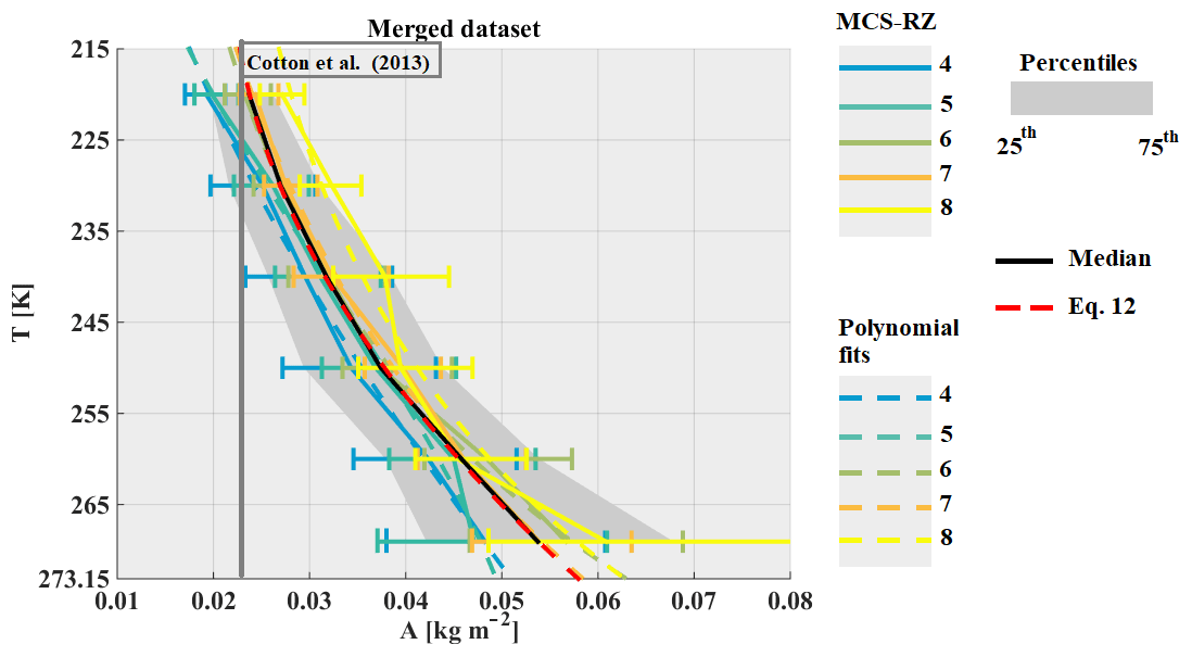
Figure 25 shows retrieved median coefficient A for the merged dataset as a function of MCS reflectivity zones and T. Note that A is calculated in SI units (in Eq. (11) IWC it is in kg m⁻³). The solid black line gives the median of A as a function of T, thereby merging all MCS reflectivity zones for the merged dataset with IWC > 0.1 g m⁻³. The grey band gives the corresponding 25th and 75th percentiles of median A. In addition, calculated median A for all individual MCS reflectivity zones (in Fig. 25) is solely illustrated for zones 4 to 8 for the merged dataset as a function of T. In general, the median A calculated for individual MCS reflectivity zones 5, 6, and 7 is very similar to the median A when merging all MCS reflectivity zones (solid black line), whereas median A calculated for MCS reflectivity zone 4 tends to have smaller A values and median A calculated for MCS reflectivity zone 8 has larger median A values than the overall median A (all MCS reflectivity zones merged) for comparable temperatures.

However, when taking into account the variability in median A calculated for individual MCS reflectivity zones and the associated 25th and 75th percentiles, we can state that median A generally increases with T. However, it is not possible to assess whether A increases with MCS reflectivity zones or IWC at constant temperature. As a comparison, we include the value of the pre-factor α (in SI unity) from the Cotton et al. (2013) mass–size relationship (β=2.0, as it is for second-moment M₂, and α=0.0257). Clearly, α=0.0257 is not suited for deep convective systems as it represents ice crystals for T∈ [215 K; 225 K[.

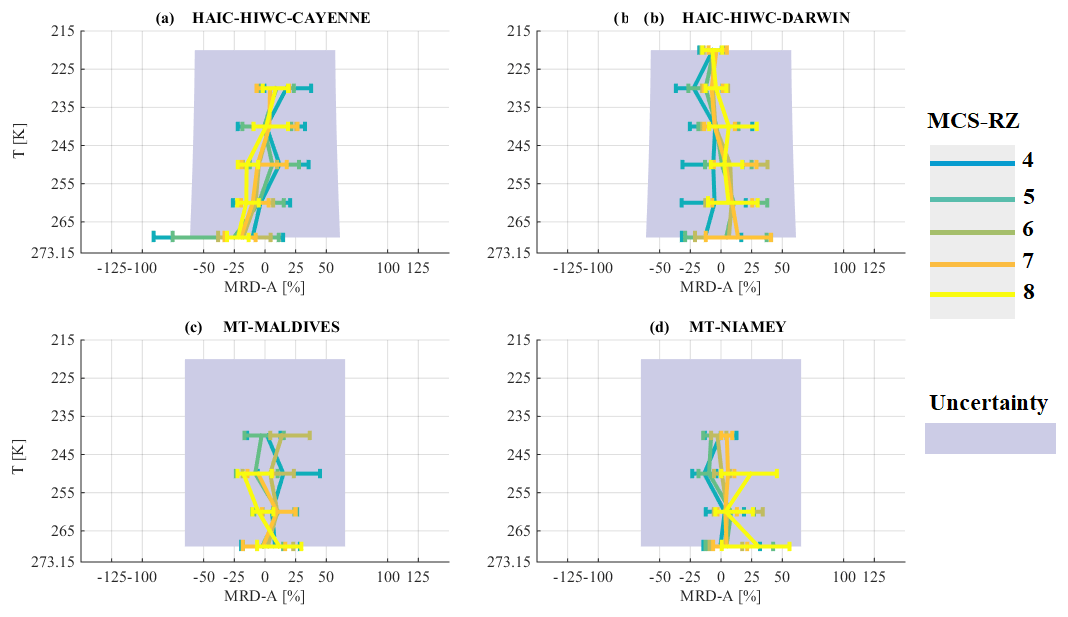
Figure 26a–d illustrates that MRD-A is significantly smaller than U(A)∕A (same uncertainty as α: U(α)/$\mathit{\alpha }=U\left(A\right)/A)$, with median MRD results centered around 0 %. Comparing results of A (Fig. 26) with results presented for α (Fig. 15, Sect. 5.4) it is obvious in terms of variability and MRD in each type of MCS that A is better adapted to parametrize the PSD second moment as a function of T. Equation (12) fits the median of ratio A for the merged dataset (dashed red line, all MCS reflectivity zones merged), as a function of T in deep convective systems for IWC larger 0.1 g m⁻³:

$$\begin{array}{ll}{\displaystyle }A\left(T\right)=& {\displaystyle }\mathrm{0.0000075}\cdot T^{\mathrm{2}}-\mathrm{0.0030598}\cdot T\\ \text{(12)}& {\displaystyle }& {\displaystyle }+\mathrm{0.3334963}\left[\mathrm{kg}{\mathrm{m}}^{-\mathrm{2}}\right].\end{array}$$

Figure 26 The same as Fig. 6 but for the ratio MRD-A.

Hence, Field et al. (2007) proposed retrieving the third-moment M₃ as a function of M₂ and T. These equations are recalled here with (in our case n=3)

$$\begin{array}{}\text{(13)}& M_n=M_{\mathrm{2}}^{F\left(n\right)}\cdot D\left(n\right)\cdot \exp \left(E\right(n)\cdot T_c).\end{array}$$

T_c denotes temperature in ^∘C and D(n), E(n), and F(n) are given by

$$\begin{array}{}\text{(14)}& {\displaystyle }D\left(n\right)& {\displaystyle }=\exp (\mathrm{13.6}-\mathrm{7.76}\cdot n+\mathrm{0.479}\cdot n^{\mathrm{2}}),\text{(15)}& {\displaystyle }E\left(n\right)& {\displaystyle }=-\mathrm{0.0361}+\mathrm{0.0151}\cdot n+\mathrm{0.00149}\cdot n^{\mathrm{2}},\text{(16)}& {\displaystyle }F\left(n\right)& {\displaystyle }=\mathrm{0.807}+\mathrm{0.00581}\cdot n+\mathrm{0.0457}\cdot n^{\mathrm{2}}.\end{array}$$

Figure 27 provides median relative errors (whiskers represent the 25th and 75th percentiles) of parameterized moments M₂ (Fig. 27a and b) and M₃ (Fig. 27c and d) compared to respective moments calculated directly (Eq. 9) from PSD measurements (merged dataset). These relative errors are shown as a function of IWC (Fig. 27a and c) and as a function of T (Fig. 27b and d). Firstly, the red line shows the median relative error of M₂ retrieved from Eq. (12) compared to M₂ derived from measured PSD (Eq. 9). In addition, the grey band illustrates the uncertainty U(M₂)∕M₂. Figure 27a illustrates that below 2 g m⁻³, the median of this relative error is close to 0 %, with the 25th and 75th percentiles being significantly smaller than U(M₂)∕M₂. However, for the largest IWC beyond 2 g m⁻³, median relative errors are increasing in size (40 % for 4 g m⁻³ and 75 % for 4.5 g m⁻³) and need to be corrected in order to reduce the bias between predicted M₂ and observed M₂. This is why Eq. (11) is modified with an expression shown in Eq. (17) in order to improve prediction of M₂ compared to measured M₂ (Eq. 10) for the highest IWC:

$$\begin{array}{}\text{(17)}& M_{\mathrm{2}}={\displaystyle \frac{\text{IWC}}{A\left(T\right)}}\cdot \exp (\mathrm{0.005853}\cdot \exp (\mathrm{1025}\cdot \text{IWC}\left)\right)\left[{\mathrm{m}}^{-\mathrm{1}}\right].\end{array}$$

The effect of the expression added in Eq. (17) is illustrated by the blue line in Fig. 27a and b, where median relative error of predicted M₂ is now also closer to 0 % for large IWC. Note that in Fig. 27b median relative errors of the two above parameterizations (solid red and blue line) of M₂ are superposed as a function of T with a median relative error close to 0 %. This means that the second part of Eq. (17) does not introduce any significant bias as a function of T, since the occurrence of IWC > 2 g m⁻³ is smaller than 1 % for the merged dataset.

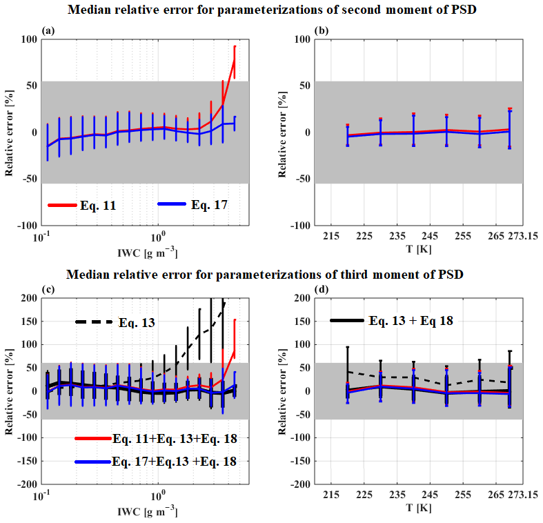
Figure 27 Relative error of parameterized M₂ and M₃ for the merged dataset as a function of IWC in (a) and (c) and as a function of T in (b) and (d). The solid lines give the median relative error and the whiskers denote the 25th and 75th percentiles of relative error. The grey band shows measurement uncertainties for M₂ (55 %; a and b) and M₃ (61 %; c and d), respectively.

In Fig. 27c and d median relative error for parameterizations of the third moment is shown, where the median relative error for all parameterization is calculated as a function of measured M₃. First, we discuss the median relative error for parametrization of third-moment M₃ according to Field et al. (2007) (Eq. (13); dashed black lines) using the measured M₂. Hence, we can see that the parameterization of Field et al. (2007) overestimates M₃ for IWC larger than 1 g m⁻³ and this overestimation of M₃ increases with IWC. Moreover, this overestimation of M₃ tends to decrease a bit as a function of T.

To reduce the significant median relative error in measured M₃, particularly for large IWC in deep convective cloud systems, we provide a M₃ correction function for Eq. (13) as a function of T and IWC:

$$\begin{array}{ll}{\displaystyle }{M}_{\mathrm{3}}=& {\displaystyle }[-\mathrm{5.605}-\mathrm{1.059}\cdot \log (\text{IWC})+\mathrm{0.009536}\cdot T\\ {\displaystyle }& {\displaystyle }-\mathrm{0.0418}\cdot \log (\text{IWC}{)}^{\mathrm{2}}+\mathrm{0.0007889}\cdot \text{log}(\text{IWC})\cdot T]\\ \text{(18)}& {\displaystyle }& {\displaystyle }\cdot M_{\mathrm{2}}^{F\left(\mathrm{3}\right)}\cdot D\left(\mathrm{3}\right)\cdot \exp \left(E\right(\mathrm{3})\cdot T_c).\end{array}$$

Following this, we discuss the three series of median relative error of M₃ where M₃ are computed with Eq. (18). First, Eq. (18) is used with measured M₂ (black solid lines) to show the efficiency of the correction applied as a function of IWC and T and described in Eq. (18). Second, Eq. (18) is applied to M₂ calculated using Eq. (11) where there is no correction as a function of IWC to calculate M₂ (red solid lines). We observe that M₃ are overestimated for IWC larger than 3 g m⁻³ and that there is no bias as a function of T with median relative error close to 0 %. Finally, Eq. (18) is used to compute M₃ from M₂ calculated with Eq. (17) when the impact of large IWC is taken into account. We can see median relative error close to 0 % for the third example of the parameterization (i.e., Eq. 17 and Eq. 18) with no bias as a function of IWC and T.

An identical investigation into median relative errors in the prediction of second and third moment as presented in Fig. 27 has been performed for individual MCS locations (figures not shown). For all types of tropical MCS, we observe that M₂ from Eq. (17) and M₃ from Eq. (18) tend to have smaller or similar median relative errors compared to the relative uncertainties U(M₂)∕M₂ and U(M₃)∕M₃, respectively. Beyond this general statement there are two noticeable observations. The first observation is that median relative errors of M₃ from Eq. (18) calculated either with M₂ from measurements (Eq. 9) or from parameterized M₂ from Eq. (17) for MCS over the Maldives are close to U(M₃)∕M₃ with 75th percentiles reaching 100 % for IWC in the range [0.3; 0.6] g m⁻³. The second observation is that for MCS over Niamey, M₃ from Eq. (18) with M₂ from Eq. (9) or from Eq. (17) tend to overestimate the respective moments calculated directly from PSD measurements by about 30 or 50 % in the area of higher IWC ([2; 3] g m⁻³).

This section aims to produce parameterizations of the second and third moments of ice hydrometeor size distributions, which can be useful for the calculation of hydrometeor size distributions in numerical weather prediction using gamma distributions but also (see the next section) for calculating rescaled ice hydrometeor size distributions (Field et al., 2007).

6.2.3 Rescaling of measured ice hydrometeors size distributions

From bulk properties as mixing ratio and total concentration in numerical weather prediction (NWP), ice hydrometeors size distributions (or PSD) properties can be derived from moment parameterization, allowing simplified prediction of cloud microphysical processes such as precipitation. Usually, ice hydrometeor size distributions are modeled by gamma distributions (Heymsfield et al., 2013; McFarquhar et al., 2007). Since the method of gamma distribution is relatively well documented, we focus this study on another type of PSD parameterization, which studies “rescaled PSD” dealing with a “mean diameter” defined by the ratio of the third moment over the second moment.

In this section, we propose an update for the method proposed by Field et al. (2007) for deep convective cloud systems and IWC larger than 0.1 g m⁻³. For the entire dataset of this study we therefore apply the method using Eqs. (19) and (20) to calculate function Φ_2,3(x) and x for individual measured PSD:

$$\begin{array}{}\text{(19)}& {\mathrm{\Phi }}_{\mathrm{2},\mathrm{3}}\left(x\right)=N\left(D_{\text{max}}\right)\cdot {\displaystyle \frac{M_{\mathrm{3}}^{\mathrm{3}}}{M_{\mathrm{2}}^{\mathrm{4}}}},\end{array}$$

with x being the characteristic size:

$$\begin{array}{}\text{(20)}& x=D_{\text{max}}\cdot {\displaystyle \frac{M_{\mathrm{2}}}{M_{\mathrm{3}}}}={\displaystyle \frac{D_{\text{max}}}{L_{\mathrm{2},\mathrm{3}}}},\end{array}$$

Φ_2,3(x) and x are dimensionless functions. Moreover, Field et al. (2007) deduced Φ_2,3(x) from their dataset, depending on cloud location, i.e., tropical troposphere or midlatitude troposphere (here we focus on the equation established for the tropics):

$$\begin{array}{ll}{\displaystyle }\text{tropics:}{\mathrm{\Phi }}_{\mathrm{2},\mathrm{3}}\left(x\right)=& {\displaystyle }\mathrm{152}\cdot \exp (-\mathrm{12.4}\cdot x)+\mathrm{3.28}\cdot x^{-\mathrm{0.78}}\\ \text{(21)}& {\displaystyle }& {\displaystyle }\cdot \exp (-\mathrm{1.94}\cdot x).\end{array}$$

Hence, the variability of PSD in clouds is not given by Φ_2,3(x) but by the variability of the second and third moments, which allow retrieving functions x and Φ_2,3(x). Following this, knowing x, Φ_2,3(x), M₂, and M₃, concentrations of ice hydrometeors can be parameterized as follows:

$$\begin{array}{}\text{(22)}& D_{\text{max}}=x\cdot {\displaystyle \frac{M_{\mathrm{3}}}{M_{\mathrm{2}}}},\end{array}$$

and

$$\begin{array}{}\text{(23)}& N\left(D_{\text{max}}\right)={\mathrm{\Phi }}_{\mathrm{2},\mathrm{3}}\left(x\right)\cdot {\displaystyle \frac{M_{\mathrm{2}}^{\mathrm{4}}}{M_{\mathrm{3}}^{\mathrm{3}}}}.\end{array}$$

Figure 28 shows the probability distribution function (PDF) of observed rescaled PSD in tropical MCS as a function of the x parameter. The thick black line represents Φ_2,3(x) from Field et al. (2007), the dashed thin grey line represents the median of Φ_2,3(x) for a given range of x with the whiskers showing the 25th and 75th percentiles of Φ_2,3(x). The figure illustrates that Eq. (21) from Field et al. (2007) represents Φ_2,3(x)rather well as a function of x in the highest PDF region (light yellow area) and fits the median plot well for x∈ [0.3; 6]. However, Field et al. (2007) performed their study for diameter larger than 100 µm, while this study calculates rescaled PSD for D_max larger than 15 µm for the underlying dataset. Thus, Eq. (21) does not fit median Φ_2,3(x) for x smaller than 0.3. In addition, for x>6, Eq. (21) decreases too quickly compared to the median of Φ_2,3(x) calculated for the global tropical dataset of this study, although Field et al. (2007) considered ice hydrometeors up to 2 cm, while this study only extrapolates PSD to 1.2845 cm (reconstruction of partial images to calculate particle size, following Korolev and Sussman, 2000). A likely assumption that could explain the differences in large x>6 might be that the merged dataset of this study may have measured PSD with the largest hydrometeors at a far higher frequency than was the case for the dataset of Field et al. (2007).

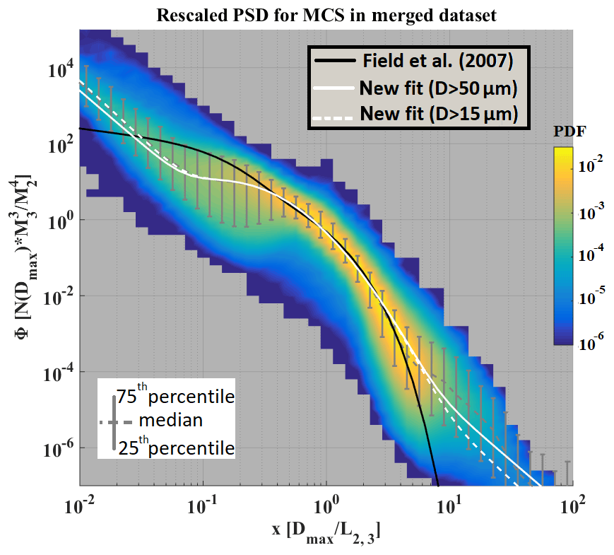
Figure 28 Probability distribution function of rescaled PSD (Φ_2,3) on the y axis as a function of hydrometeor characteristics size (x) on the x axis for the merged datasets. The black lines show fitted functions from Field et al. (2007), the dotted grey lines show the median rescaled PSD with an error bar from the 25th and 75th percentiles of rescaled PSD. The solid white line shows the new fitted function for the merged dataset for PSD beyond 55 µm, and the dashed white line shows the fitted function for PSD beyond 15 µm (Eq. 24).

White lines (dashed and solid) show new fitted Φ_2,3(x) for the merged dataset of this study. The dashed and solid white lines can be represented by the following equation and aim to fit the median (Φ_2,3(x)) of Fig. 28 as a function of x:

$$\begin{array}{ll}{\displaystyle }\text{Tropics:}{\mathrm{\Phi }}_{\mathrm{2},\mathrm{3}}\left(x\right)=& {\displaystyle }\left[\exp \left(a_{\mathrm{1}}\right)\cdot x^{a_{\mathrm{2}}}\right],\\ \text{(24)}& {\displaystyle }& {\displaystyle }+\left[b_{\mathrm{1}}\cdot \exp \left(-{\displaystyle \frac{\left(\ln \right(x)-b_{\mathrm{2}}{)}^{\mathrm{2}}}{b_{\mathrm{3}}^{\mathrm{2}}}}\right)\right],\end{array}$$

where b₁=9.484, $b_{\mathrm{2}}=-\mathrm{1.895}$, and b₃=1.083. Note that dashed and solid white lines use different sets of coefficients a₁ and a₂ (Table 1). For the dashed white line, a₁ and a₂ are calculated for D_max beyond 15 µm, whereas for the solid white line, a₁ and a₂ are calculated for D_max beyond 55 µm. We can notice that the function for D_max≥15 µm produces higher Φ_2,3(x) as compared to the function fitted for D_max≥55 µm. In order to explain this difference, we recall that for MCS over the Maldives concentrations of hydrometeors with D_max≤55 µm are higher compared to the three other tropical MCS locations, which could affect the fitted coefficients a₁ and a₂ in the two different versions of Φ_2,3(x) calculations for the merged dataset. Another difference in small particle measurements could be a pure technical difference in small particle measurements (including shattering, out-of-focus, and small-sample-volume artifacts) between the 2D-S probe (this study) and 2D-C probe (Field et al., 2007).

Table 1 Coefficients a₁ and a₂ for Eq. (24).

The parameterization developed in this study is performed on ice hydrometeor distributions defined as a function of D_max. However, NWP usually assumes that ice hydrometeors are spherical. Thus, Appendix E explores the impact of assuming that ice hydrometeors are spherical in the context of this study, noting that volumes of ice hydrometeors recorded by OAP are not directly measured. This latter short study was performed by supposing that the correct method for defining ice hydrometeor distribution might be around using D_max or spherical diameter. For both assumptions there is a need to perform sensitivity studies to assess which parameterization is more suited for NWP.

7 Discussion and conclusion

In this study we analyze in situ aircraft observations of ice hydrometeor images and simultaneous cloud radar observations collected in tropical MCS in order to characterize the statistical properties of ice microphysics. The results are focused on the tropical MCS that include observations from (i) the rainy season over Cayenne (South America), (ii) the North Australian Monsoon over Darwin, (iii) deep convective systems over Maldives in the ITCZ, and (iv) the West African Monsoon over Niamey.

The overall data analysis of ice hydrometeor properties has been performed as a function of temperature and the range of radar reflectivity factors measured at 94 GHz. Therefore, all vertical profiles of aircraft onboard radar reflectivity measurements have been gathered and statistically analyzed in order to define delimited radar reflectivity zones, thereby reducing possible vertical bias due to the chosen flight track and altitude in the MCS systems. Hence, this study defines eight MCS reflectivity zones that have been determined from radar reflectivity factor percentiles (1st, 10th, 30th, 50th, 70th, 90th, and 99th) as a function of temperature, thereby merging all vertical reflectivity profiles of the entire merged dataset used for this study. Analysis of the retrieved vertical wind speeds in each MCS reflectivity zone reveals that the probability to observe a magnitude of vertical winds larger than 1 m s⁻¹ is similar in MCS reflectivity zones 1 to 5 but then strongly increases from MCS reflectivity zone 6 to 8. Generally, these probabilities increase with decreasing temperature for all MCS reflectivity zones. Additionally, the simple magnitude of vertical wind speeds is larger in MCS reflectivity zones 7 and 8, while in MCS reflectivity zones 1 to 6 the magnitude is rather small and similar; however, the magnitude is a function of T. Our investigation does not allow us to directly link MCS reflectivity zones and the stage of life cycle of MCS (i.e., formation, maturation, decaying). However, the analysis of geostationary satellite data would be more suited for this topic (Fiolleau and Roca 2013). Following this, studying the distribution of MCS reflectivity zones as a function of life cycle of MCS, brightness temperature, and/or visible reflectance could help to answer to this question.

However, this study demonstrates that MCS reflectivity zones 7 and 8 exhibit the highest probability of being related to the active convective zone and/or the most turbulent transition zone between the inaccessible part of the convective core and the stratiform part of MCS clouds, whereas MCS reflectivity zones 1 to 5 are instead associated with the so-called stratiform parts of MCS. MCS reflectivity zone 6 thus represents the transition between the stratiform and convective area of MCS with relatively small median magnitudes of vertical winds but with a relatively high probability of vertical wind magnitudes beyond 1 m s⁻¹.

Subsequently, the study compares microphysical properties (e.g., ice water content, extinction, concentrations, largest hydrometeor sizes) as a function of MCS reflectivity zone and temperature. The statistical analysis (median values and 25th and 75th percentiles) is performed for the individual MCS locations, whereas the merged dataset of the four tropical MCS locations serves as a reference. Relative differences between median microphysical properties in one MCS location and respective median properties of the reference dataset were quantified. Uncertainties for all types of microphysical measurements and retrieved cloud parameters were also calculated from Baumgardner et al. (2017).

Within the range of uncertainties, we showed that the variability of IWC, σ, N_T,50, N_T,500, M₂, and M₃ as a function of temperature and specific MCS reflectivity zones tends to be similar. For example, for IWC these conclusions apply for MCS reflectivity zones 4 to 8. MCS data from the Niamey flight campaign (compared to the three other tropical MCS locations) reveal more exceptions when compared with median parameters calculated for the global tropical dataset, with a trend of larger third PSD moments and larger hydrometeor sizes in the stratiform area of MCS. Assuming that largest hydrometeors (max(D_max)) can be considered a proxy for the aggregation process efficiency, the findings of this study reveal that aggregation process efficiency is higher for MCS over land than over islands and higher over islands close to large land masses than over islands in the middle of an ocean. It seems to confirm the results of Frey et al. (2011) and Cetrone and Houze (2009).

From the tropical dataset a parametrization of visible extinction has been developed as a function of temperature and IWC (Eq. 8). This model allows for retrieving σ from OAP measurements with an accuracy smaller than the measurement uncertainty of σ ($U\left(\mathit{\sigma }\right)/\mathit{\sigma }=\mathrm{57}\mathit{\%}$; Eq. 2) for all four types of tropical MCS. Eq. (8) reveals the best accuracy for representing directly calculated σ in MCS over Darwin and Niamey.

Also in this study, the relationship between mass and size of ice hydrometeors ($m=\mathit{\alpha }\cdot D^{\mathit{\beta }}$) is formulated with a classical power law approximation. A basic finding is that the variability of retrieved β throughout all MCS reflectivity zones is too large compared to its uncertainty. This would mean, for example, that varying β parameterization in NWP is not worth doing. Indeed, NWP schemes are used to describe ice microphysics with PSD moments (here M₂ and M₃). Setting β=2 for the mass–size relationship allows us to link IWC to the second moment directly as stated in Field et al. (2007).

Defining A as the ratio IWC∕M₂, this study illustrates that A increases with temperature. A in MCS reflectivity zones 5, 6, and 7 is also similar to the median A calculated for the entire dataset (Fig. 16a). In MCS reflectivity zone 4 (smaller zones were not considered), A tends to be smaller, and in MCS reflectivity zone 8, A tends to be larger than the median of A for the merged dataset. However, MCS reflectivity zones 4 and 8 share a wide range of variability with MCS reflectivity zones 5, 6, and 7. Hence, we use the variability of A as a function of temperature (parametrization in Eq. 12) to predict the second PSD moment in tropical MCS. Whereas Eq. (11) retrieves M₂ in all types of MCS with a good accuracy, a correction is needed for high IWC (Eq. 17).

Hence, in this study the model of PSD moments presented by Field et al. (2007) has been considerably modified for PSD in deep convective clouds systems in order to predict the third moment (M₃) from the known second moment (M₂), IWC, and temperature T. This new parametrization of M₃ for deep convective clouds systems and IWC larger than 0.1 g m⁻³ is given by Eqs. (12), (17), and (18). The prediction of M₂ (Eq. 17) is more accurate than the prediction of M₃ (Eq. 18), when compared with M₂ and M₃ directly calculated from the measured PSD. Indeed, the predicted M₂ have median relative errors in the range [−25 %; 25 %] (corresponding to the 25th and 75th percentiles of relative error of M₂) with an uncertainty of measured M₂ of about 55 %. The predicted M₃ have median relative errors in the range [−40 %; 55 %] (which corresponds to the 25th and 75th percentiles of relative error of M₃) with an uncertainty of measured M₃ of 61 %. Note that the use of this parameterization might lead an underestimation of the third moments of PSD in NWP of the stratiform part of West African Monsoon's MCS.

Furthermore, we applied the method of Field et al. (2007) on the four tropical datasets of PSD rescaled with the second and third moments of the measured PSD.

For their dataset Field et al. (2007) gave a parameterized function Φ_2,3 that models rescaled PSD in the tropics as a function of the mean diameter (ratio between the third moment and the second moment of the PSD). The calculated rescaled PSD for the four tropical datasets is in good agreement with Φ_2,3 parametrization given by Field et al. (2007) from diameters between 0.3 and 6 times the mean diameter (dimensionless characteristic size x). At 0.3 times the mean diameter, Φ_2,3 of Field et al. (2007) tends to overestimate the rescaled PSD and finally underestimates them again below 0.03 times the mean diameter. These differences can be explained by the different diameter threshold used to calculate the rescaled PSD. In our study, we calculate rescaled PSD starting at 15 µm (or 50 µm; see Table 1 and Eq. 24), while Field et al. (2007) used PSD only beyond 100 µm. For large mean diameters we also note significant differences between the rescaled PSD for the dataset of this study and Φ_2,3 parametrization from Field et al. (2007). Indeed, for diameters larger than 6 times the mean diameter, Φ_2,3 of Field et al. (2007) decreases rapidly and therefore underestimates the rescaled PSD by about an order of magnitude at diameters equal to 10 times the mean diameter. We do not think that these differences are due to the difference in the cutoff diameter of PSD (the last available diameter for PSD), which was 20,000 µm in Field et al. (2007) versus 12,845 µm in this study. Field et al. (2007) used PSD of ice hydrometeors measured in anvils and cirrus clouds, while the entire dataset for this study has been gathered closest to MCS stratiform and convective zones of deep convective systems.

This latter fact more than likely explains differences between the rescaled PSD of this study and parameterized Φ_2,3 from Field et al. (2007). The underlying dataset for this study probably contains more large hydrometeors in non-negligible concentrations and related increased statistics on large hydrometeor concentrations.

The parametrization based on tropical PSD data beyond 15 µm seems to degrade parametrization results for the largest diameters (rescaled concentrations beyond parametrization). We suspect that this is due to very high concentrations of small hydrometeors in the range 15–55 µm in MCS over the Maldives, which would finally suggest recommending the parametrization for tropical MCS solely based on PSD beyond 50 µm in order to retrieve ice properties in deep convective clouds that could serve in NWP.

To conclude on the parameterization of ice hydrometeor distribution, we performed an update of the computation of PSD as a function of IWC and T performed by Field et al. (2007) for tropical convective clouds (see Eqs. 11, 17 and 18). This parameterization was used in the microphysical scheme based on Wilson and Ballard (1999) used in the configuration of the Met Office Global Atmosphere version 6.1 (Walters et al., 2017), which was the version of the Unified Model used operationally by the Met Office for global weather and climate prediction. More precisely, the ice and snow concentrations were computed with the moment parameterization developed by Field et al. (2007) and the mass–diameter relationship from Cotton et al. (2013). Here, we suggest using the new parameterization developed in our study for ice and snow concentrations when IWC are larger than 0.1 g m⁻³. Otherwise, we suggest keeping either the original version of the Field et al. (2007) parameterization with the Cotton et al. (2013) mass–size relationship or the original version of Field et al. (2007) parameterization with A as a function of temperature, which would be a fit of the 25th percentile of A in MCS reflectivity zone 4 (see Table C12 in Appendix C).

We showed that IWC tends to be similar as a function of temperature and MCS reflectivity zone, suggesting that the IWC–Z–T relationship developed by Protat et al. (2016) would be applicable for IWC larger than 0.1 g m⁻³ in tropical MCS. In other words there is a confident relationship between IWC, Z, and T in tropical MCS. Following this, for the evaluation of NWP, we suggest defining the MCS reflectivity zones using the 25th percentiles of IWC as the lower limit of each MCS reflectivity zone (see Table C2 in Appendix C). Hence, for each MCS reflectivity zone visible extinction, hydrometeors concentrations (NT₅₀, NT₅₀₀, M₂, and M₃), reflectivity factors at 94 GHz, and vertical velocities from NWP can be compared with the findings of this study (see Table in Appendix C). This methodology should help to identify where NWP fails to represent the links between different parameters and IWC. Indeed, studying the spatiotemporal variability of IWC in MCS is a complex topic. It needs a time reference and a space reference. For MCS, the time reference can be its life cycle, but there are MCS that have a more complex life cycle than others (merging of MCS, a new growing stage after a decaying stage). Concerning the space reference, there is a common view, which is to observe the MCS from its most active area, i.e., its convective part. There are two difficulties to take into account here. First, there are very few direct measurements of cloud microphysics in the very convective area of MCS. Second, MCS can be the aggregation of many convective cells that can be well organized or poorly organized (Houze, 2004). Moreover, we saw that large IWC tend to be more associated with vertical movement than lower IWC, but this is not always true.

To test NWP of extreme weather events such MCS, we suggest using the statistic performed in this study, by testing the different conditions of others microphysical parameters observed for a given IWC and temperature.

Finally, several findings from this study suggest more investigations into the variability of the relationship between projected surface and mass of ice hydrometeors encountered in underlying observations are required. Indeed, we find that ice “density” is similar as a function of T and Z reflectivity ranges in all four MCS locations. Hence, this is referring to the possibility of investigating a surface–mass relationship in MCS that should be a function of T and Z(IWC). Estimating that aerosol loads and corresponding cloud condensation nuclei and IN properties may be more or less different in these four locations (continental aerosol over Africa with a strong influence of dust from Sahara, cleaner troposphere over the Indian ocean, merging of continental and oceanic influences), we stipulate the need for investigating secondary ice production processes that seem to regulate the concentrations of ice hydrometeors beyond 55 µm.

Appendix A: Total concentrations for D_max>15 µm

Figure A1 shows median total concentration (N_T) as a function of T and MCS reflectivity zone for the merged datasets where concentrations of ice hydrometeors are integrated beyond 15 µm:

$$\begin{array}{}\text{(A1)}& N_T=\sum _{D_{\text{max}}=\mathrm{15}}^{D_{\text{max}}=\mathrm{12845}}N\left(D_{\text{max}}\right)\cdot \mathrm{\Delta }{D}_{\text{max}}\left[{\mathrm{L}}^{-\mathrm{1}}\right].\end{array}$$

Median N_T systematically increases with MCS reflectivity zone and altitude, but there is significant overlap of the 25th and 75th percentiles of neighboring MCS reflectivity zones. Measurement uncertainty in concentrations given for small hydrometeors is about ± 100 % (Baumgardner et al., 2017).

Figure A2a–d shows MRD-N_T of MCS in the different tropical locations. For MCS over Darwin and Cayenne, in all MCS reflectivity zones MRD-N_T are smaller than the measurement uncertainty, whereas for Niamey data this is the case only in MCS reflectivity zones 2, 5, 6, and 7. MCS over the Maldives yield significantly larger MRD-N_T than the measurement uncertainty, and those are primarily positive. Hence, MCS over the Maldives have larger concentrations of hydrometeors for a same range of T and Z than the three other types of tropical MCS. However, these larger concentrations observed do not concern zones where highest concentrations of hydrometeors were observed. For example, in MCS reflectivity zone 4 where MRD-N_T reaches 1000 %, N_T for the Maldives dataset is approximately 1000 L⁻¹, which is similar to N_T observed in MCS reflectivity zones 7 and 8 for the same range of T∈ [235 K; 245 K[ for the merged dataset. We recall that identical image data processing to remove shattering artifacts and to correct out-of-focus images (Field et al., 2003; Korolev and Isaac, 2005; Leroy et al., 2016) has been applied for all four tropical datasets. The presence of supercooled droplets has also been investigated (RICE, CDP probe), and a few periods with supercooled water content have been removed for this study. Moreover, we show in Sect. 5.5 that MCS over the Maldives tend to have smaller max(D_max), especially in MCS reflectivity zones 4, 5, 6, and 7, when compared to the other MCS locations and that concentrations beyond 500 µm in the Maldives observations are in the same range as the other types of MCS.

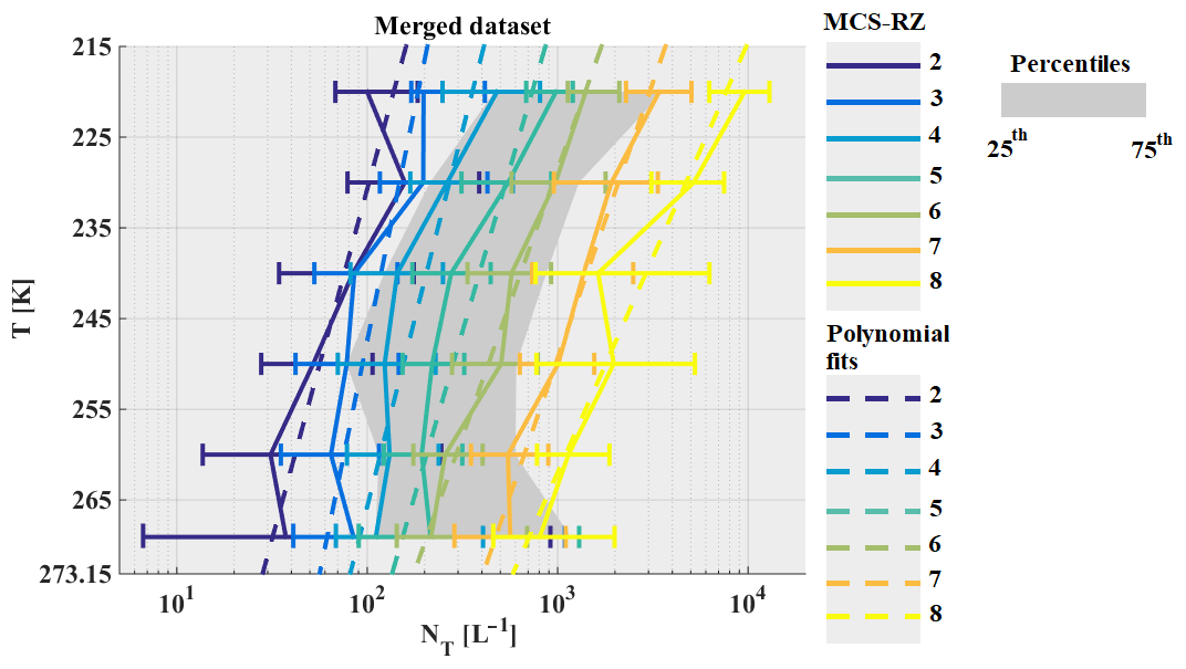
Figure A1 The same as Fig. 5 but for concentrations of hydrometeors integrated beyond D_max=15 µm in L⁻¹.

Figure A2 The same as Fig. 6 but for MRD-NT.

Appendix B: Impact of updraft and downdraft on median relative errors

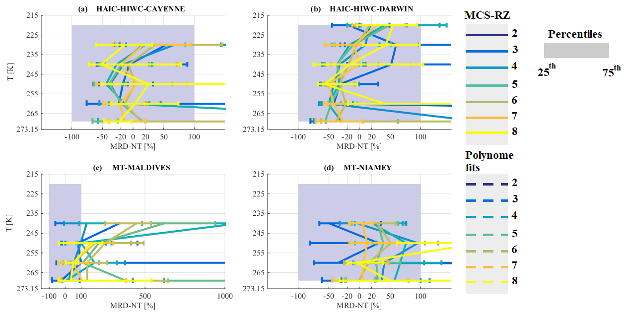
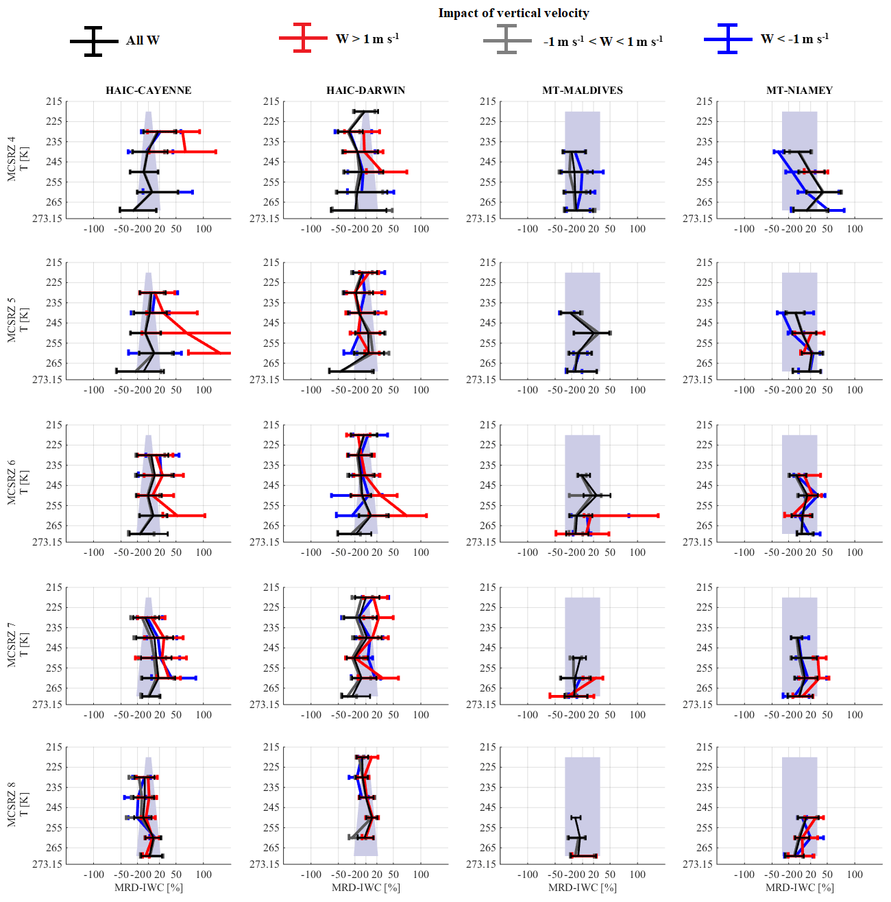
Figure B1 Median relative difference of IWC (MRD-IWC) in regard to median IWC calculated for the merged dataset in each MCS reflectivity zone (Fig. 5). Results are sorted as a function of MCSRZ 4 (top line) to MCSRZ 8 (bottom line). The blue lines represent MRD-IWC for vertical velocity smaller than −1 m s⁻¹. The grey lines represent MRD-IWC for vertical velocity larger than −1 m s⁻¹ and smaller than 1 m s⁻¹. The red lines represent MRD-IWC for vertical velocity larger 1 m s⁻¹. The black lines represent MRD-IWC when there is no distinction as a function of vertical velocity (as in Fig. 6a–d).

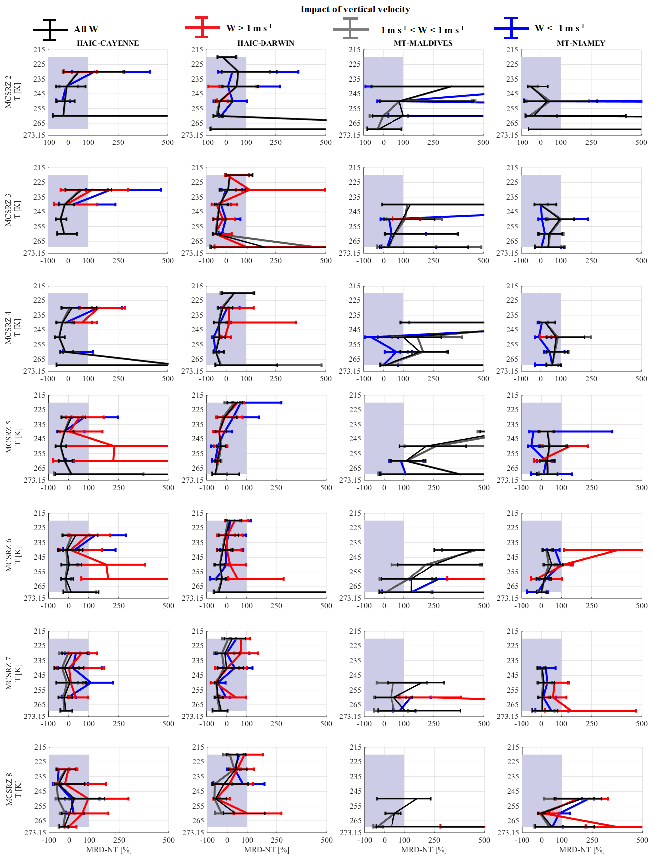
Figure B2 Median relative difference of total concentration of hydrometeors (MRD-NT) in regard to median total concentrations calculated for the merged dataset in each MCS reflectivity zone (Fig. A1). Results are sorted as a function of MCSRZ 2 (top line) to MCSRZ 8 (bottom line). The blue lines represent MRD-NT for vertical velocity smaller than −1 m s⁻¹. The grey lines represent MRD-NT for vertical velocity larger than −1 m s⁻¹ and smaller than 1 m s⁻¹. The red lines represent MRD-NT for vertical velocity larger 1 m s⁻¹. The black lines represent MRD-NT when there is no distinction as a function of vertical velocity (as in Fig. A2a–d).

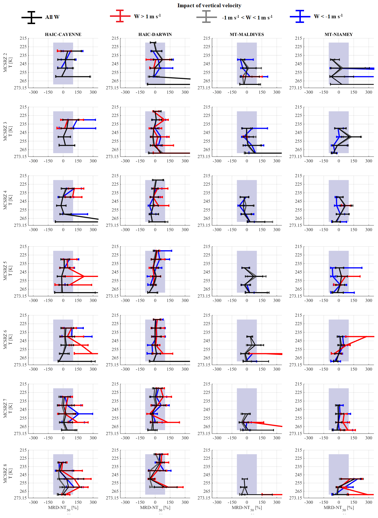
Figure B3 Median relative difference of concentration of hydrometeors summed over D_max for D_max larger than 50 µm (MRD-NT₅₀) in regard to median total concentrations calculated for the merged dataset in each MCS reflectivity zone (Fig. 9). Results are sorted as a function of MCSRZ 2 (top line) to MCSRZ 8 (bottom line). The blue lines represent MRD-NT₅₀ for vertical velocity smaller than −1 m s⁻¹. The grey lines represent MRD-NT₅₀ for vertical velocity larger than −1 m s⁻¹ and smaller than 1 m s⁻¹. The red lines represent MRD-NT₅₀ for vertical velocity larger 1 m s⁻¹. The black lines represent MRD-NT₅₀ when there is no distinction as a function of vertical velocity (as in Fig. 10a–d).

Appendix C: Tables

Table C1 Percentile of radar reflectivity factors (Z) in dBZ, shown as a solid line in Fig. 1.

Table C2 Ice water content (IWC) in g m⁻³ (Fig. 5).

Table C3 Visible extinction (σ) in m⁻¹ (Fig. 7).

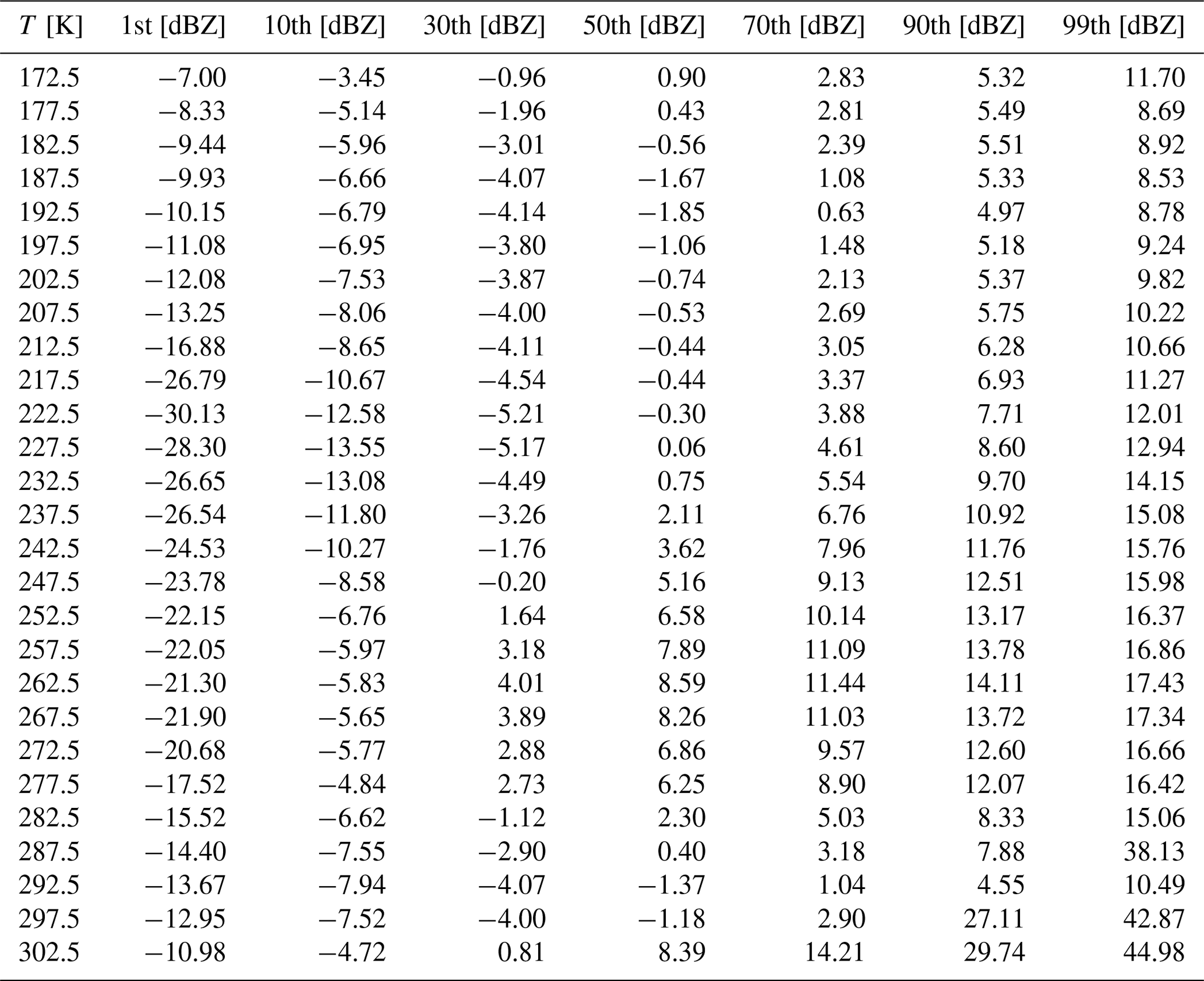
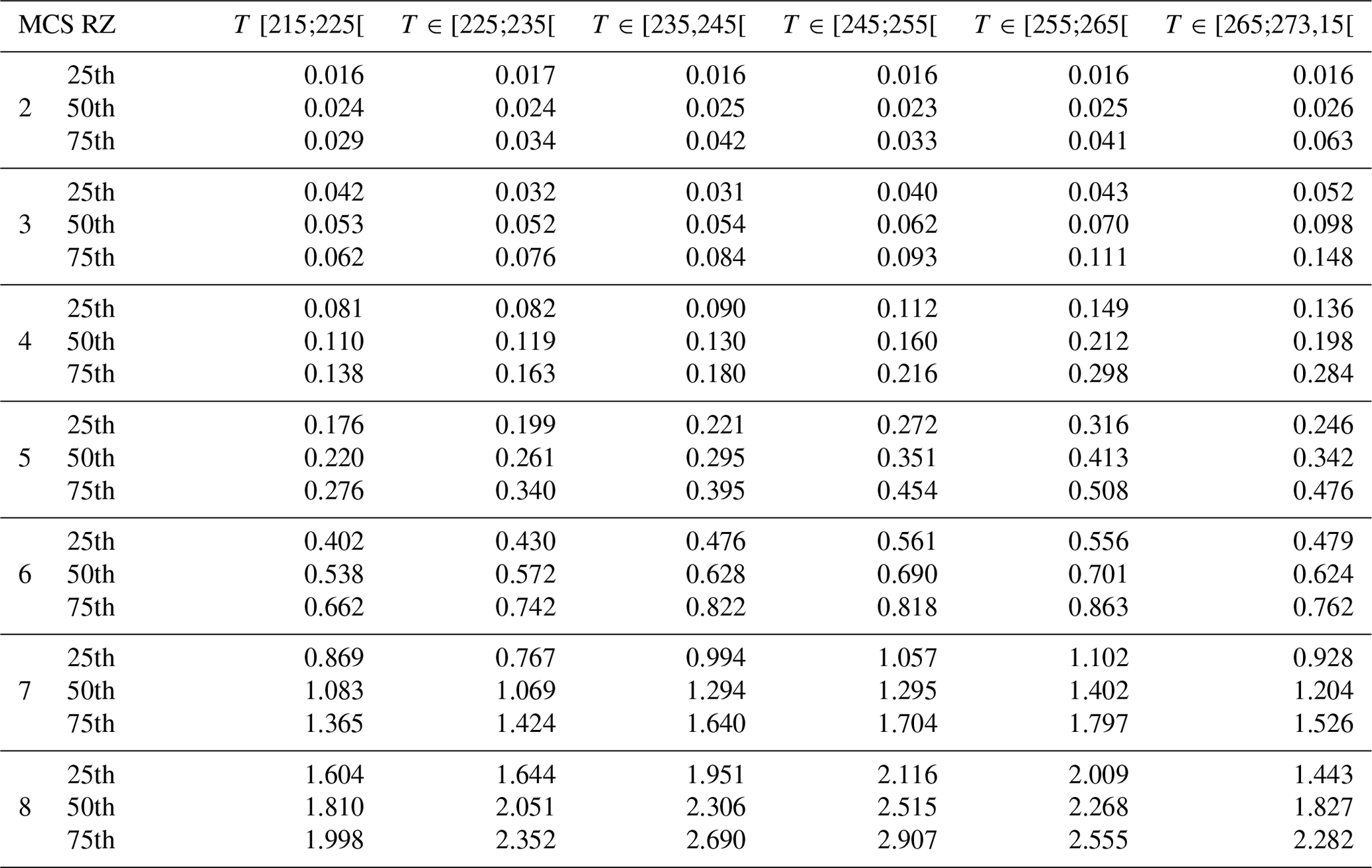
Table C4 Total concentration beyond 15 µm (N_T) in L⁻¹ (Fig. A1).

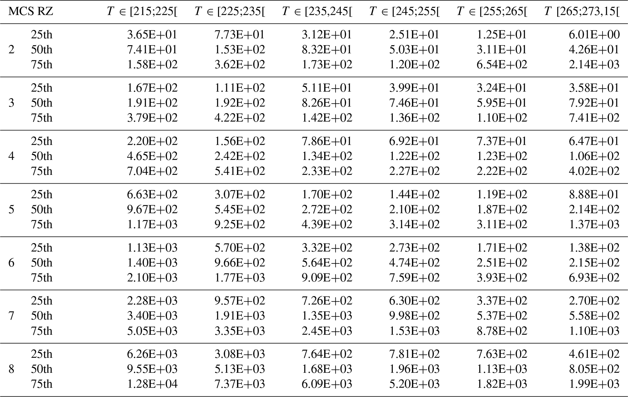
Table C5 Total concentration since 50 µm (N_T 50) in L⁻¹ (Fig. 9).

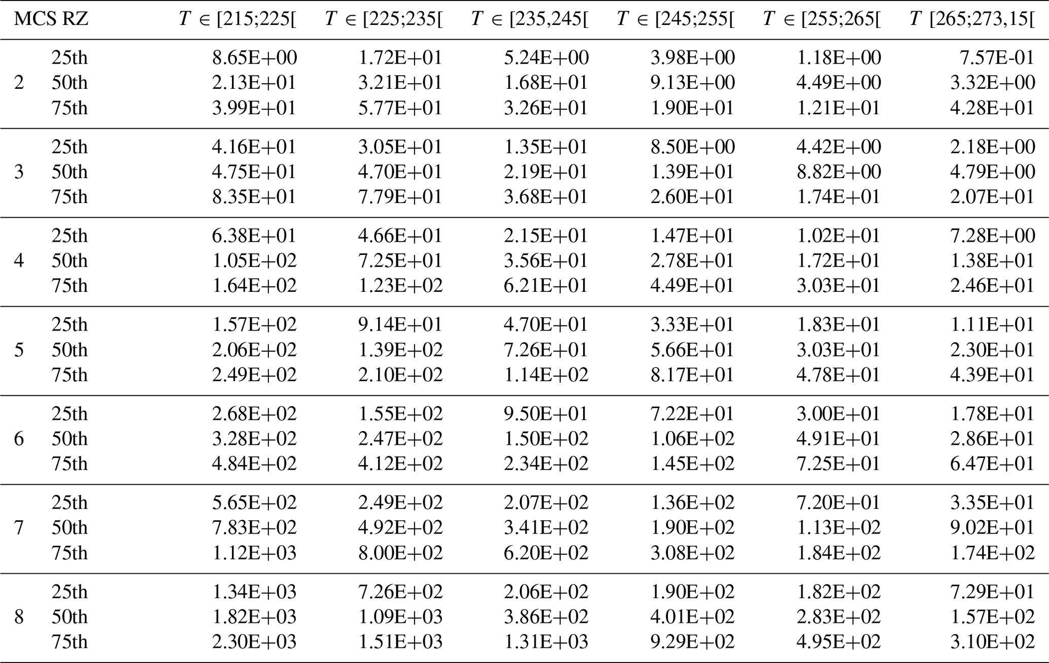
Table C6 Total concentration from 500 µm (N_T 500) in L⁻¹ (Fig. 11).

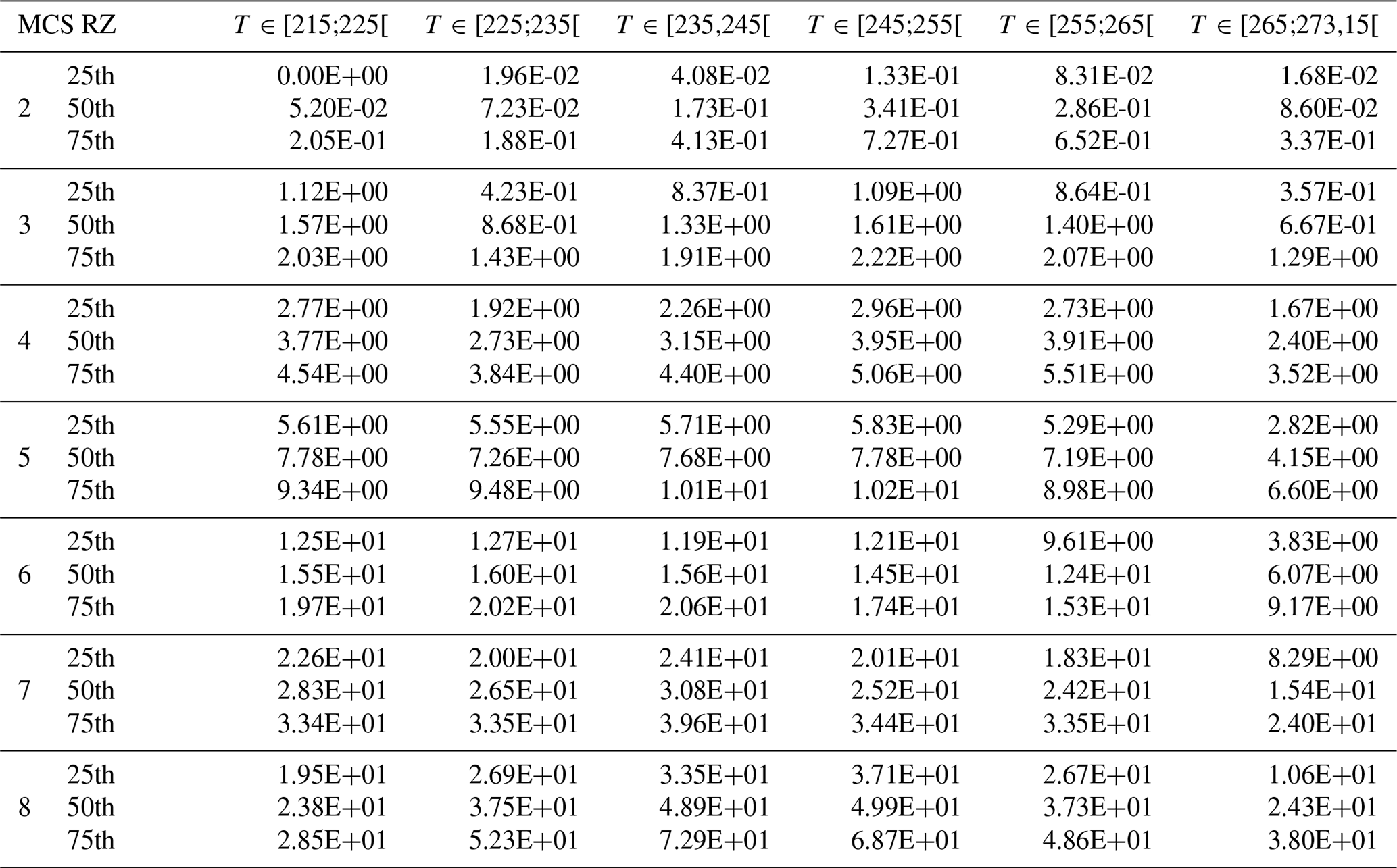
Table C7 Pre-factor α of mass–size relationship in g cm^−β (Fig. 15).

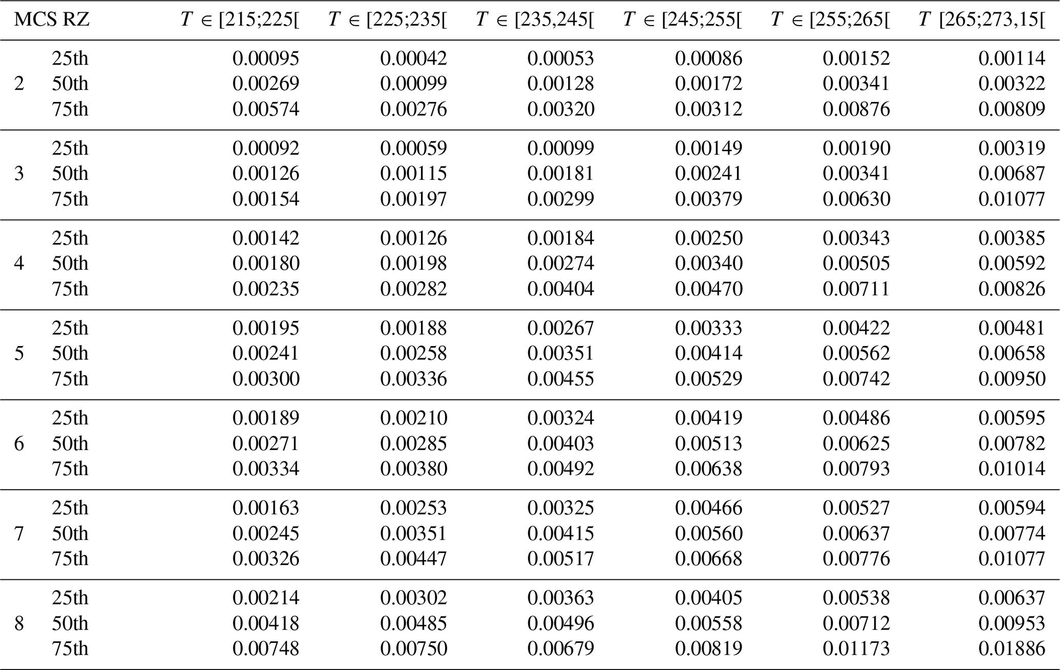
Table C8 Exponent of mass–size relationship β (no dimension) (Fig. 13).

Table C9 The max(D_max) in cm (Fig. 17).

Table C10 The second moment of PSD (M₂) in m⁻¹ (Fig. 21).

Table C11 The third moment of PSD (M₃; no dimension)(Fig. 23).

Table C12 Coefficient A in kg m⁻² (Fig. 25).

Appendix D: Summary of intercomparison of ice microphysical properties in MCS.

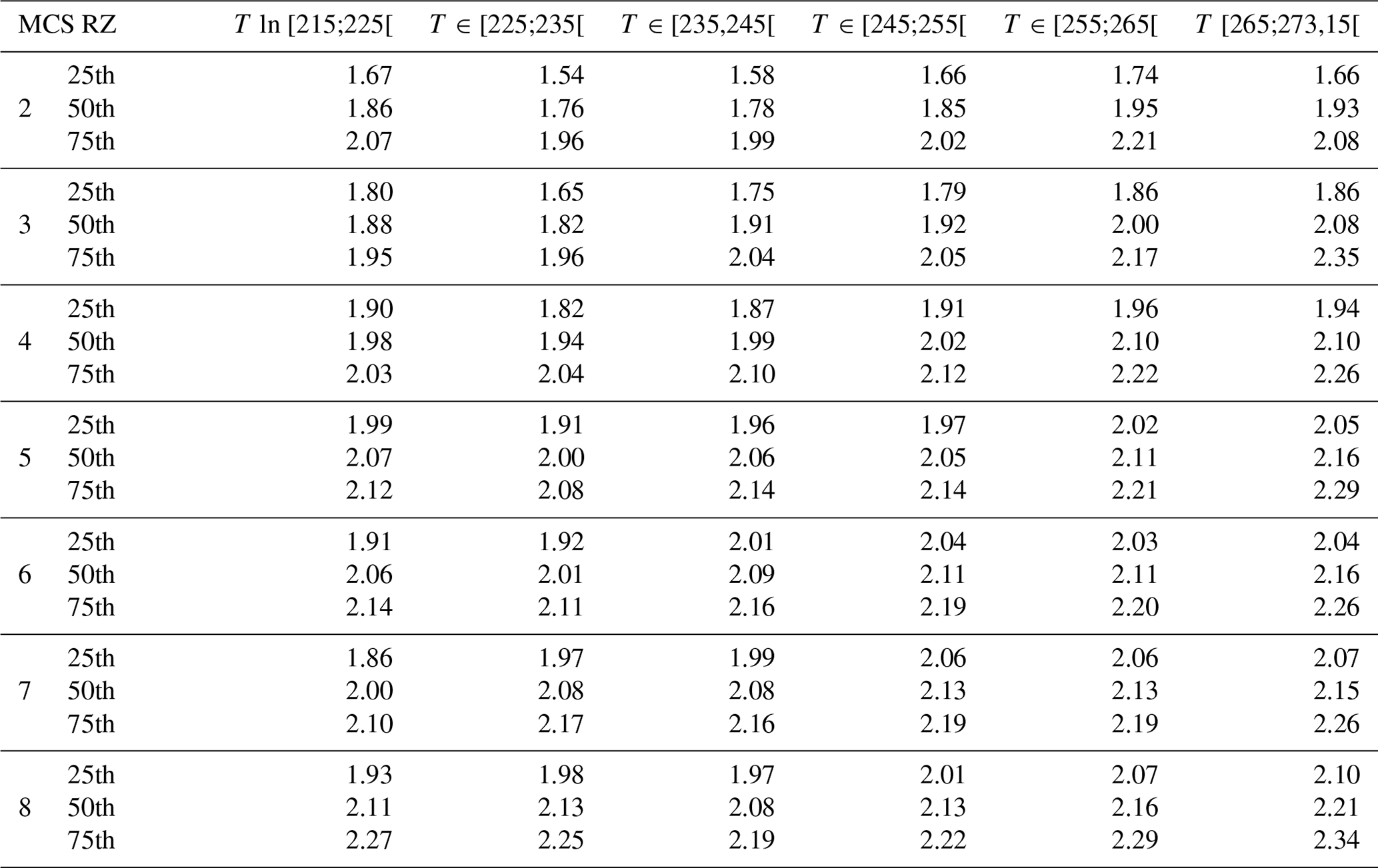
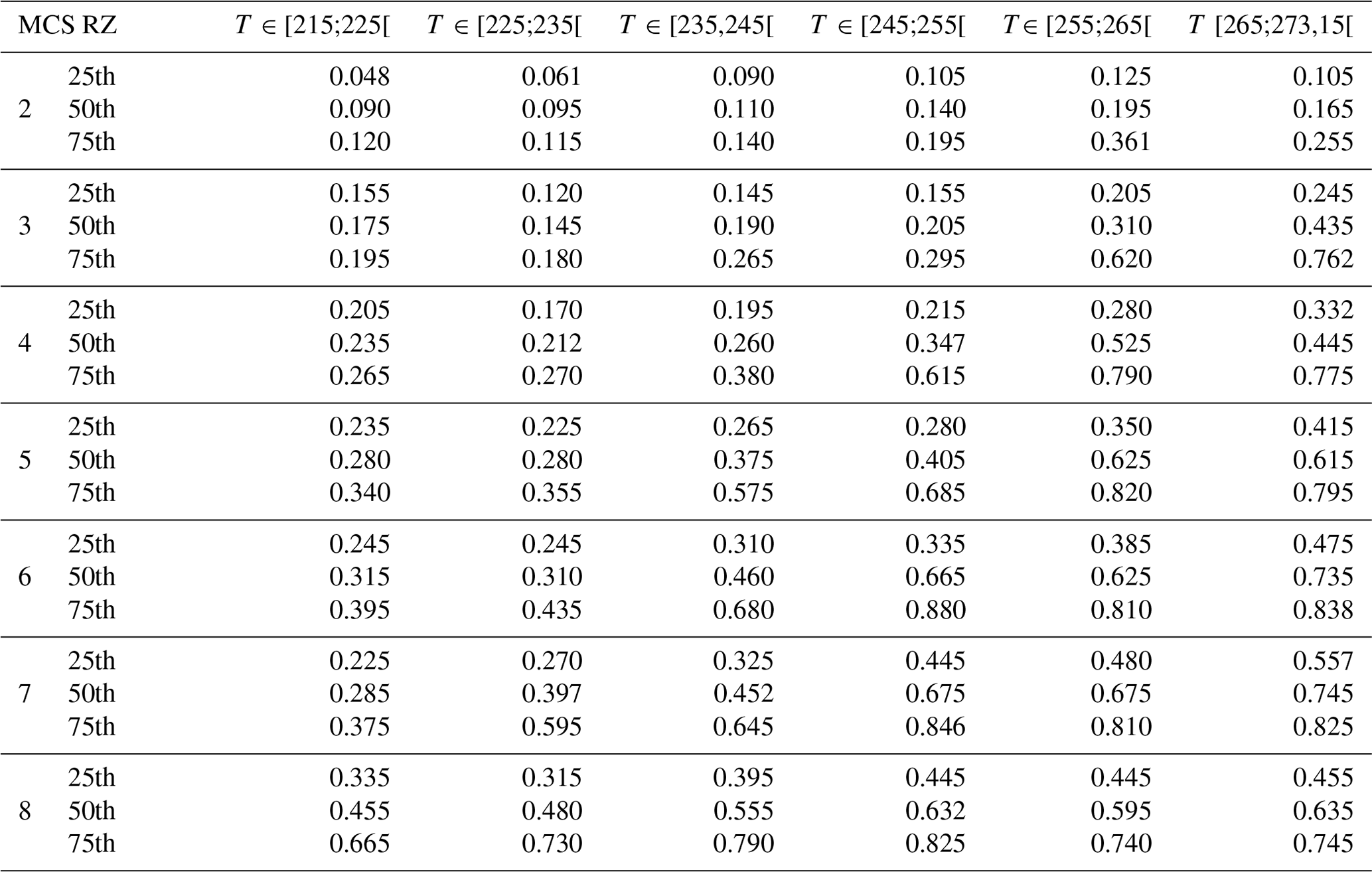
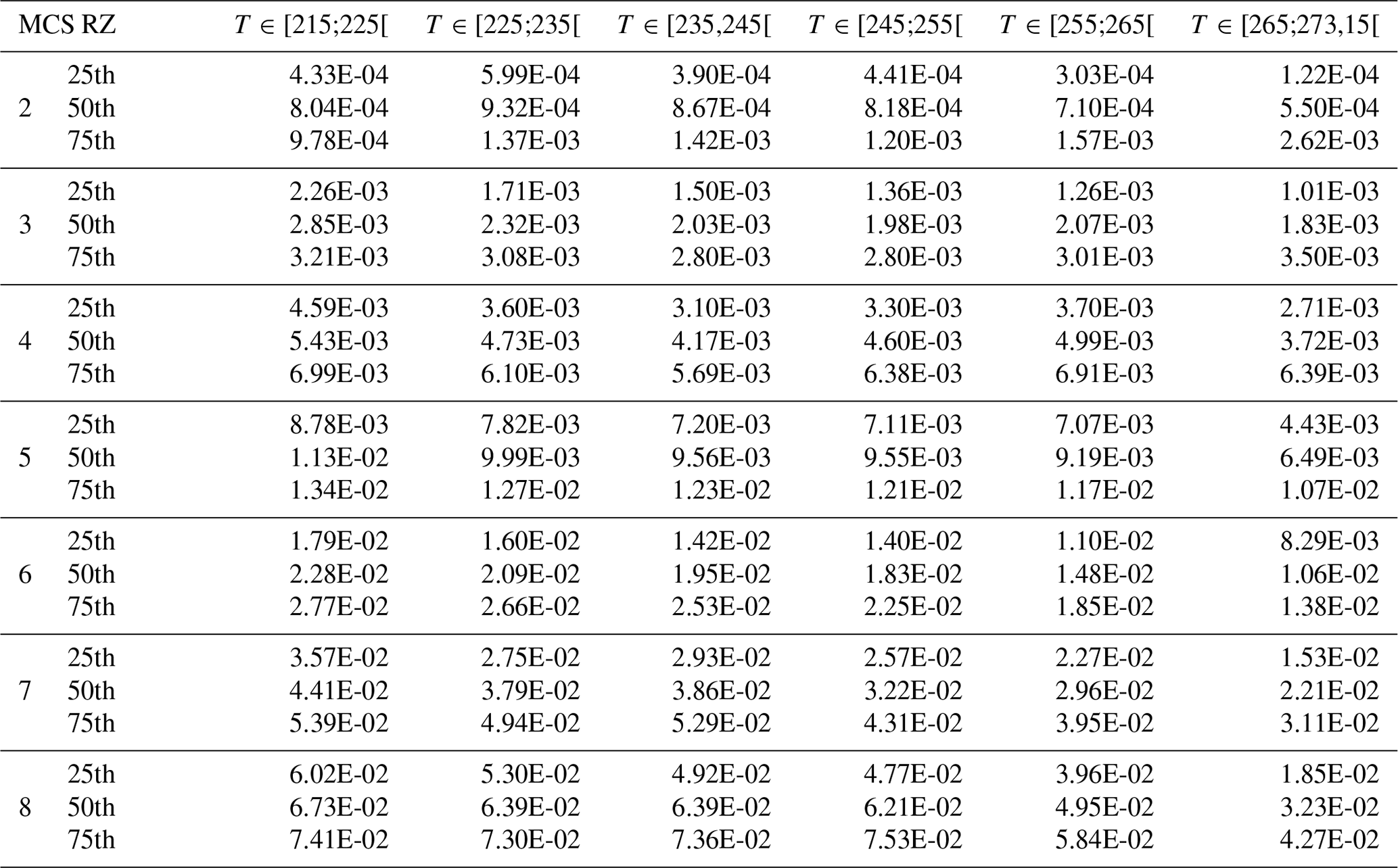
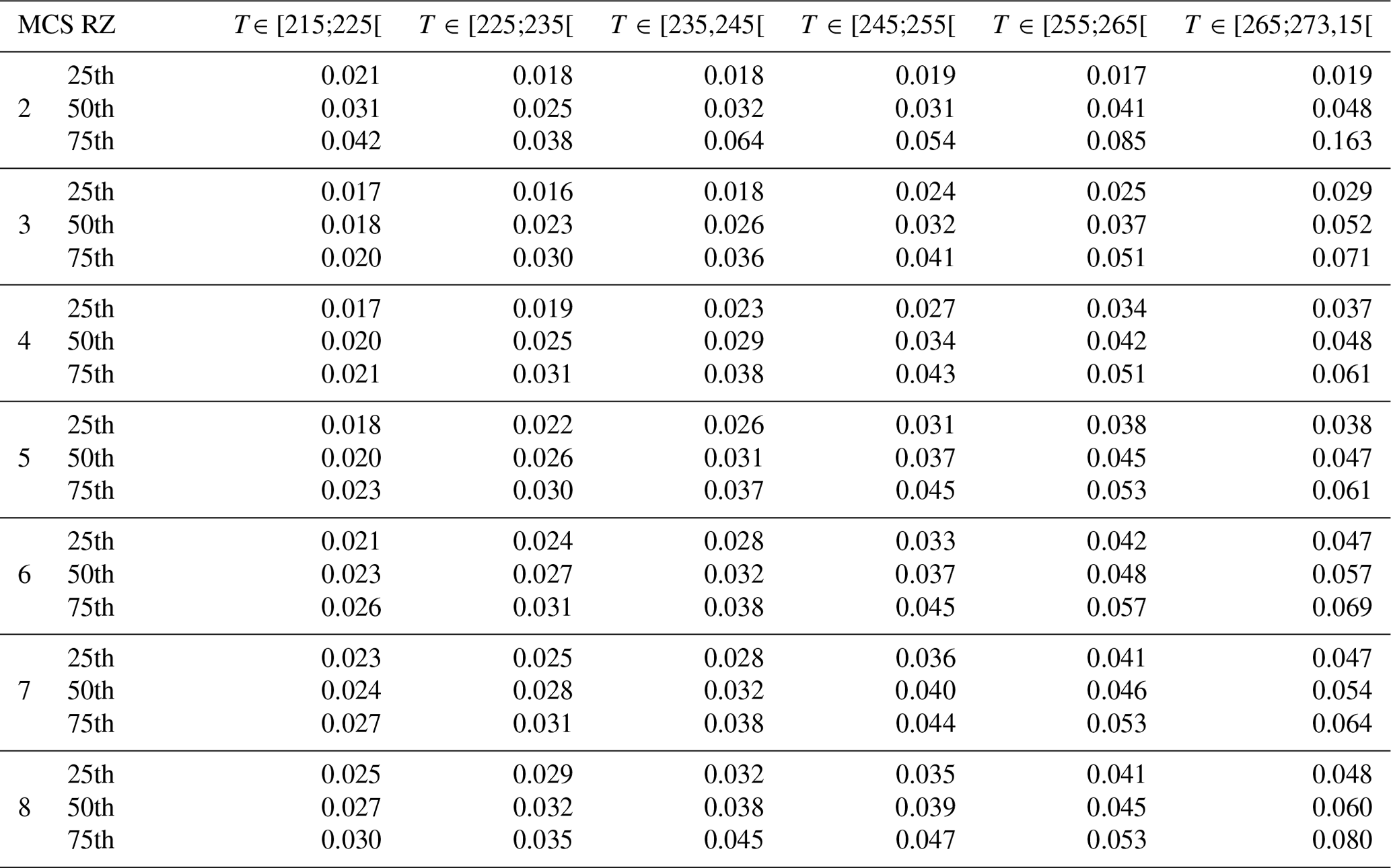
Table D1 qualitatively summarizes the findings for IWC, visible extinction (σ), total concentrations (N_T,50 for D_max>50 µm; N_T,500 for D_max>500 µm), second moment (M₂) and third moment (M₃) of hydrometeor PSD, and the largest hydrometeors sizes (max(D_max)). It highlights the main tendencies of microphysical parameters in each type of MCS with regards to the median calculation performed for the merged dataset, i.e., ≅ for similar values, + for larger values and – for smaller values than the merged dataset. Additionally, this shows the exceptions, noting their location as a function of the temperature range and the MCS reflectivity zones.

Table D1 Evaluation of parameter X (X for IWC, σ, N_T,55, N_T,500, M₂, M₃, and max(D_max)) for each type of tropical MCS (Darwin, Cayenne, the Maldives, Niamey) with respect to the global tropical dataset, thereby comparing median values in corresponding MCS reflectivity zones. There are two sub-columns for each type of MCS: the first column gives an evaluation of the main trend (≅ if MRD-X is comparable to the uncertainty range, + if MRD-X is larger than the uncertainty range, – for smaller values). In the second sub-column the number of exceptions with respect to the main trend (first column) are reported: Z(Y)≅, Z(Y)+, or Z(Y)–. Z number stands for a particular MCS reflectivity zone (with Z=2, 3, 4, 5, 6, 7, 8) and Y number represents a particular T range (with Y=1 for T∈ [265 K; 273.15 K[, Y=2 for T∈ [255 K, 265 K[, Y=3 for T∈ [245 K; 255 K[, Y=4 for T∈ [235 K; 245 K[, Y=5 for T∈ [225 K; 235 K[, and Y=6 for T∈ [215 K; 225 K[).

Appendix E: Rescaled PSD parameterization for spherical equivalent diameter

Models for NWP usually use the assumption that ice hydrometeors are spherical. However, our study presents results using maximum diameter (D_max). There is a possibility that the last definition might not be adapted for NWP. We propose exploring the impact on the proposed parameterizations of PSD calculated in the main text when assuming the volume of spherical hydrometeors. First, we need to compute the volume of the hydrometeors from the in situ measurement. For that we assume that hydrometeors are oblate spheroids. It is possible from the images recorded by the OAP to deduce D_max and the width (length perpendicular to D_max). With this assumption it is possible to calculate the volume of such oblate spheroids ($V\left(D_{\text{max}}\right)=\mathrm{0.25}\cdot \mathit{\pi }\cdot \text{width}\left(D_{\text{max}}\right)\cdot D_{\text{max}}^{\mathrm{2}}$). Following this, we calculate the equivalent spherical diameter for the volume computed for this spheroid ($D_{\text{sp}}\left(D_{\text{max}}\right)=(\mathrm{6}\cdot V(D_{\text{max}})/\mathit{\pi }{)}^{\mathrm{1}/\mathrm{3}}$). For each bin of D_max there is a calculation of the mean width from all its particles and for every 5 s period, hence a D_sp(D_max). Following this, the second and third moment (M_2Dsp and M_3Dsp, respectively) of PSD can be calculated by replacing D_max in Eq. (9) with D_sp (Eq. E1).

$$\begin{array}{}\text{(E1)}& M_n=\sum _{D_{\text{max}}=\mathrm{55}\mathrm{\mu }\mathrm{m}}^{D_{\text{max}}=\mathrm{1},\mathrm{2}\mathrm{cm}}N\left(D_{\text{sp}}\right)\cdot D_{\text{sp}}^n\cdot \mathrm{\Delta }{D}_{\text{sp}}\left[{\mathrm{m}}^{n-\mathrm{3}}\right]\end{array}$$

As it is calculated on measured PSD, N(D_sp)=N(D_max) and ΔD_sp=ΔD_max. The results for the second moment of PSD are presented in Figs. E1 and E2, where Fig. E1 shows M_2Dsp and Fig. E2 shows MRD-M_2Dsp both as a function of MCS reflectivity zones and temperature. The same is true for M_3Dsp and MRD-M_3Dsp, presented in Figs. E3 and E4, respectively. For the second moment of PSD as a function of Dsp, results are similar to those for the second moment for PSD as a function of D_max, except that for a given MCS reflectivity zone M_2Dsp is about 30 % smaller than M₂ from D_max. We obtain the same conclusion for the third moment, but M_3Dsp is about 40 % to 50 % smaller than M₃ from D_max. However, MRD-M_2Dsp and MRD-M_3Dsp are similar to MRD-M₂ and MRD-M₃ from D_max.

As the second and third moments from PSD as a function of Dsp are smaller than the second moment from PSD as a function of D_max, Eqs. (12) and (18) need to be updated as follows (Figs. E5 and E6):

$$\begin{array}{ll}{\displaystyle }A\left(T\right)=& {\displaystyle }\mathrm{1.656}\times {\mathrm{10}}^{-\mathrm{5}}\cdot T^{\mathrm{2}}-\mathrm{0.0070224}\cdot T\\ \text{(E2)}& {\displaystyle }& {\displaystyle }+\mathrm{0.7780590}\left[\mathrm{kg}{\mathrm{m}}^{-\mathrm{2}}\right].\end{array}$$

Hence, Eq. (E2) is used in Eq. (17) to calculate the second moment of PSD as a function of D_sp. Following this, Eq. (E3) is used instead of Eq. (18) to calculate the third moment of PSD as a function of D_sp.

$$\begin{array}{ll}{\displaystyle }{M}_{\mathrm{3}}=& {\displaystyle }\left[-\mathrm{3.066}-\mathrm{0.6124}\cdot \log \left(\text{IWC}\right)+\mathrm{0.004251}\cdot T\right.\\ {\displaystyle }& {\displaystyle }\left.-\mathrm{0.02495}\cdot \log (\text{IWC}{)}^{\mathrm{2}}+\mathrm{0.0002413}\cdot \log (\text{IWC})\cdot T\right]\\ \text{(E3)}& {\displaystyle }& {\displaystyle }\cdot M_{\mathrm{2}}^{F\left(\mathrm{3}\right)}\cdot D\left(\mathrm{3}\right)\cdot \exp \left(E\right(\mathrm{3})\cdot T_c)\end{array}$$

Figure E7 shows the efficiency of the updated parameterization for the second and third moment of PSD as a function of D_sp. Figures E7 and 27 are similar, demonstrating that the parameterization for PSD as a function of D_sp is as accurate as the one for PSD as a function of D_max. Moreover, Fig. E8 shows that the function Φ_2,3(x)(Eqs. 19, 20, and 24) is also valid to describe PSD as a function of equivalent spherical diameter.

This appendix explores the consequences of using PSD as a function of equivalent spherical diameter (as PSD is usually described in NWP) on the parameterization of ice hydrometeor size distribution in MCS developed in the main part of this study. Of the four equations that describe this parameterization, only two equations need to be updated with new coefficients: Eq. (12) becomes Eq. (E2) and Eq. (18) becomes Eq. (E3). While Eqs. (17) and (24) are applicable to both types of PSD whether PSD is a function of D_max or a function of D_sp.

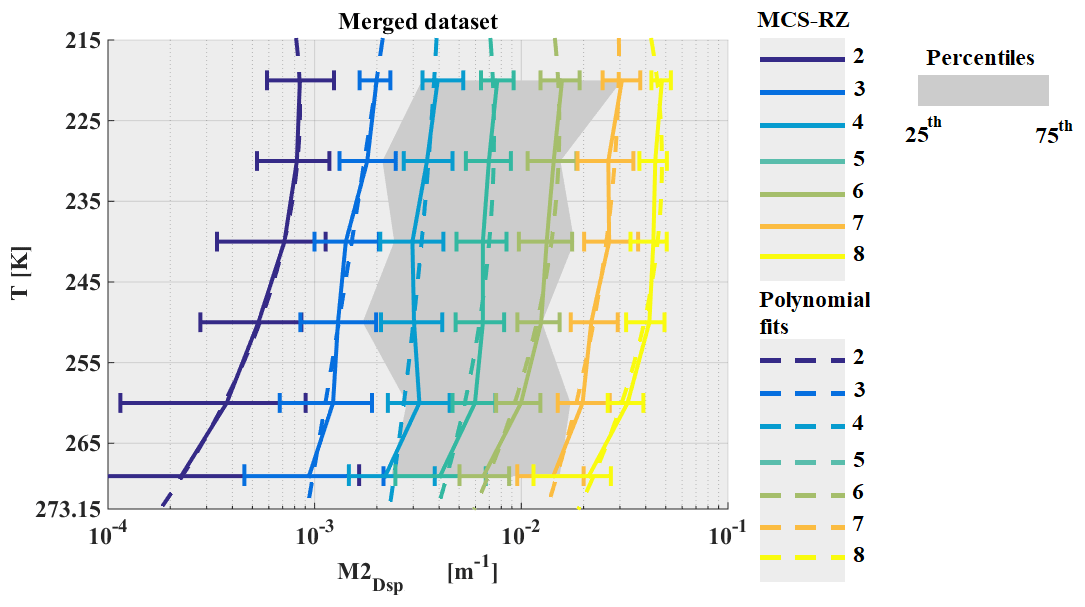
Figure E1 The same as Fig. 5 but for M_2,Dsp m⁻¹, where PSD is used as a function of equivalent spherical diameter.

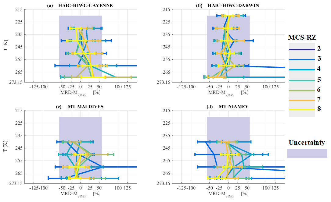
Figure E2 The same as Fig. 6 but for MRD-M_2,Dsp, where PSD is used as a function of equivalent spherical diameter.

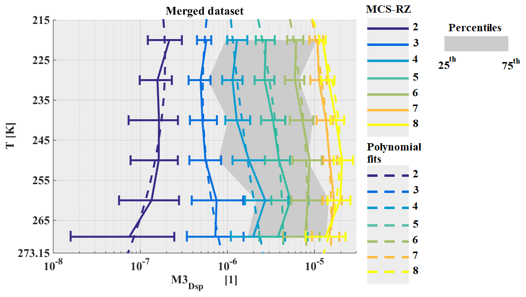
Figure E3 The same as Fig. 5 but for M_3,Dsp m⁻¹, where PSD is used as a function of equivalent spherical diameter.

Figure E4 The same as Fig. 6 but for MRD-M_3,Dsp, where PSD is used as a function of equivalent spherical diameter.

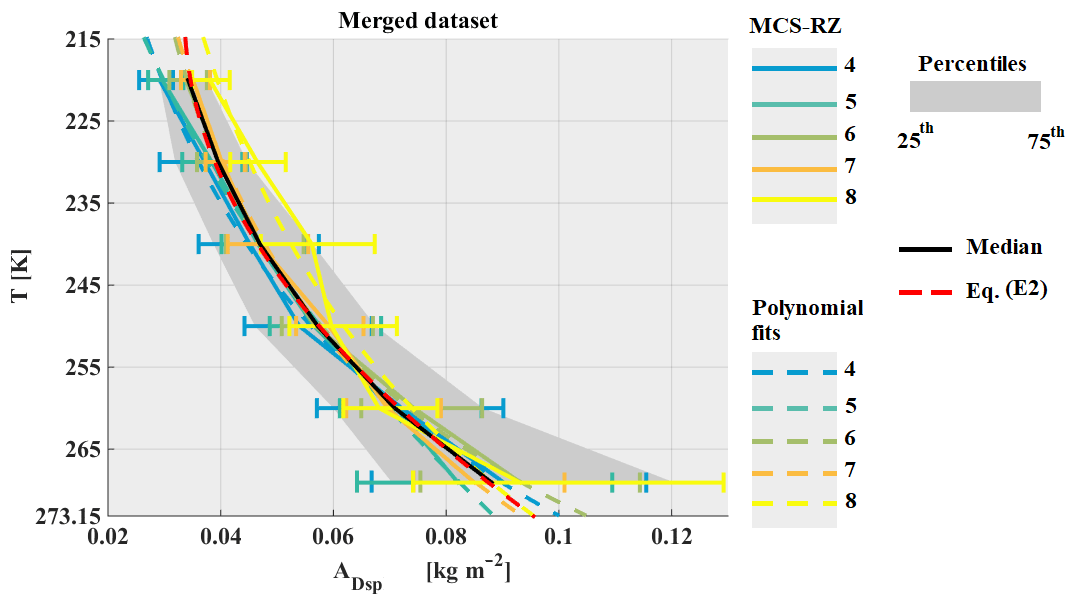
Figure E5 The same as Fig. 5 but for the ratio $A_{\mathrm{Dsp}}=\text{IWC}/M_{\mathrm{2},\mathrm{Dsp}}$ in kg m⁻², where PSD is used as a function of equivalent spherical diameter.

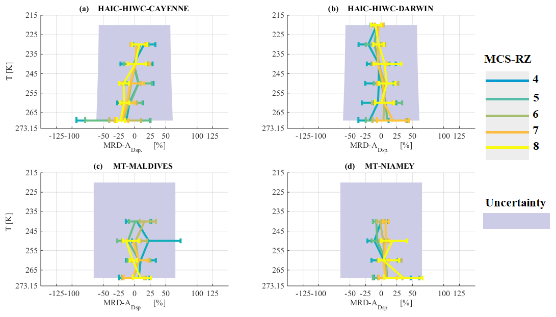
Figure E6 The same as Fig. 6 but for the ratio MRD-A_Dsp, where PSD is used as a function of equivalent spherical diameter.

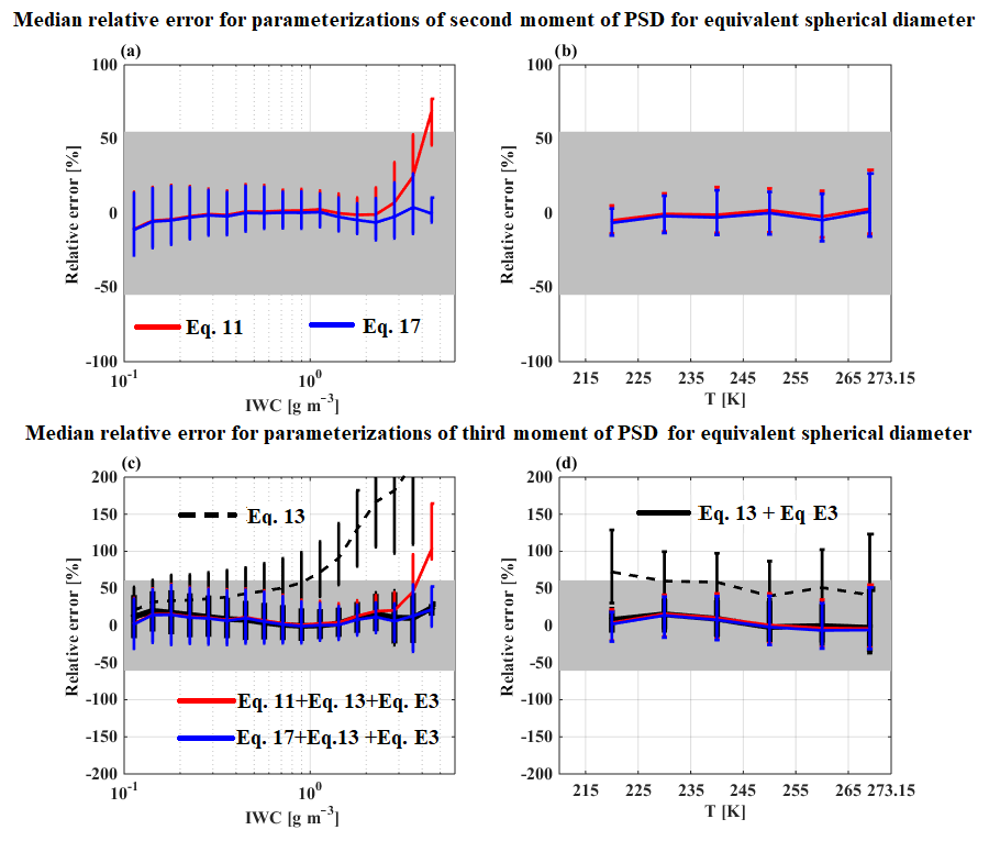
Figure E7 Relative error of parameterized M_2,Dsp and M_3,Dsp for the merged dataset as a function of IWC in (a) and (c) and as a function of T in (b) and (d). The solid lines give the median relative error and the whiskers denote the 25th and 75th percentiles of relative error. The grey bands shows measurement uncertainties for M_2,Dsp (55 %; a and b) and M_3,Dsp (61 %; c and d), respectively, for PSD as a function of equivalent spherical diameter.

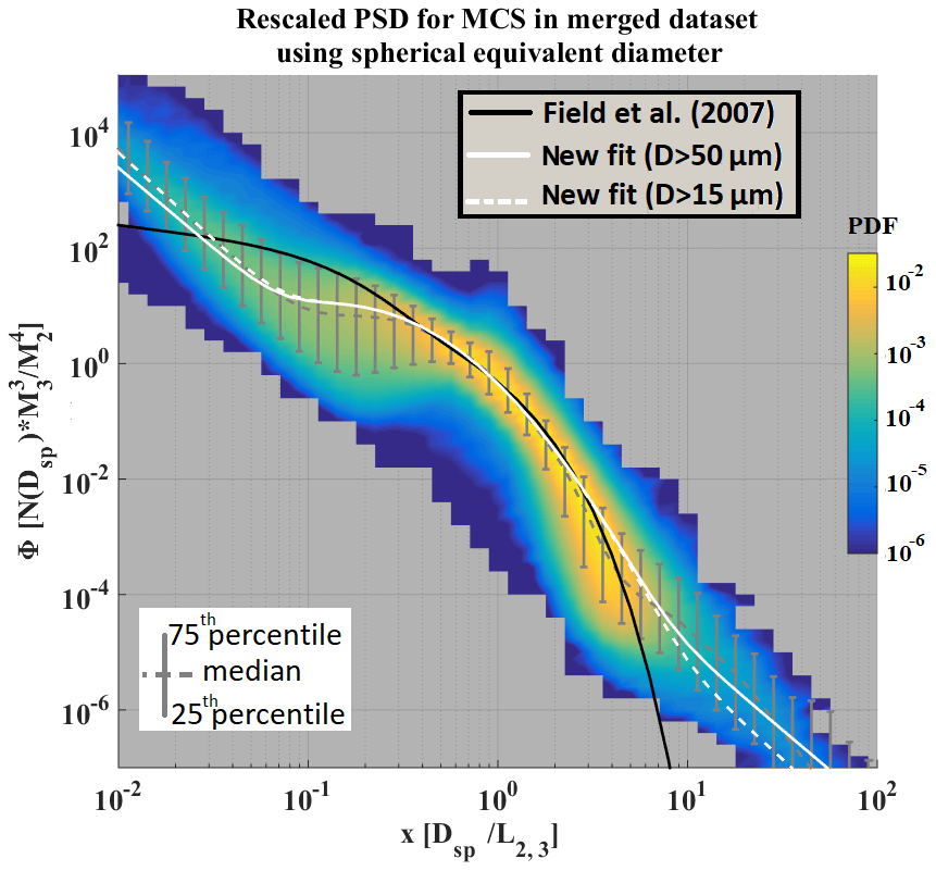
Figure E8 Probability distribution function of rescaled PSD (Φ_2,3) on the y axis as a function of hydrometeor characteristic size (x) on the x axis for the merged datasets. The black lines show fitted functions from Field et al. (2007). The dotted grey lines show the median rescaled PSD with an error bar from the 25th and 75th percentiles of the rescaled PSD. The solid white line shows the new fitted function for the merged dataset for PSD beyond 55 µm, and the dashed white line shows the fitted function for PSD beyond 15 µm (Eq. 24), when PSD are calculated as a function of equivalent spherical diameter.