the Creative Commons Attribution 4.0 License.
the Creative Commons Attribution 4.0 License.
 | 23 Mar 2020
Modeling stratospheric intrusion and trans-Pacific transport on tropospheric ozone using hemispheric CMAQ during April 2010 – Part 2: Examination of emission impacts based on the higher-order decoupled direct method
Syuichi Itahashi
Rohit Mathur
Christian Hogrefe
Sergey L. Napelenok
Yang Zhang
The state-of-the-science Community Multiscale Air Quality (CMAQ) modeling system, which has recently been extended for hemispheric-scale modeling applications (referred to as H-CMAQ), is applied to study the trans-Pacific transport, a phenomenon recognized as a potential source of air pollution in the US, during April 2010. The results of this analysis are presented in two parts. In the previous paper (Part 1), model evaluation for tropospheric ozone (O3) was presented and an air mass characterization method was developed. Results from applying this newly established method pointed to the importance of emissions as the factor to enhance the surface O3 mixing ratio over the US. In this subsequent paper (Part 2), emission impacts are examined based on mathematically rigorous sensitivity analysis using the higher-order decoupled direct method (HDDM) implemented in H-CMAQ. The HDDM sensitivity coefficients indicate the presence of a NOx-sensitive regime during April 2010 over most of the Northern Hemisphere. By defining emission source regions over the US and east Asia, impacts from these emission sources are examined. At the surface, during April 2010, the emission impacts of the US and east Asia are comparable over the western US with a magnitude of about 3 ppbv impacts on monthly mean O3 all-hour basis, whereas the impact of domestic emissions dominates over the eastern US with a magnitude of about 10 ppbv impacts on monthly mean O3. The positive correlation (r=0.63) between surface O3 mixing ratios and domestic emission impacts is confirmed. In contrast, the relationship between surface O3 mixing ratios and emission impacts from east Asia exhibits a flat slope when considering the entire US. However, this relationship has strong regional differences between the western and eastern US; the western region exhibits a positive correlation (r=0.36–0.38), whereas the latter exhibits a flat slope (r < 0.1). Based on the comprehensive evaluation of H-CMAQ, we extend the sensitivity analysis for O3 aloft. The results reveal the significant impacts of emissions from east Asia on the free troposphere (defined as 750 to 250 hPa) over the US (impacts of more than 5 ppbv) and the dominance of stratospheric air mass on upper model layer (defined as 250 to 50 hPa) over the US (impacts greater than 10 ppbv). Finally, we estimate changes of trans-Pacific transport by taking into account recent emission trends from 2010 to 2015 assuming the same meteorological condition. The analysis suggests that the impact of recent emission changes on changes in the contribution of trans-Pacific transport to US O3 levels was insignificant at the surface level and was small (less than 1 ppbv) over the free troposphere.
- Article
(10646 KB) - Full-text XML
- Companion paper
-
Supplement
(11709 KB) - BibTeX
- EndNote


Tropospheric ozone (O3) is a secondary air pollutant produced through photochemical reactions including nitrogen oxides (NOx) and volatile organic compounds (VOCs) (Haagen-Smit and Fox, 1954). Tropospheric O3 plays an important role by producing hydroxyl radicals (OH) which control the oxidizing capacity (Logan, 1985). O3 at the surface level poses significant human health impacts; hence, many countries have an air quality standard for its ambient mixing ratios. The National Ambient Air Quality Standard (NAAQS) of O3 in the US is set on the annual fourth highest maximum daily 8 h concentration (MD8O3) averaged over 3 years. Its threshold value was set at 70 ppbv in 2015 (U.S. EPA, 2018). An analysis of trends in surface O3 observation during the periods of 1998 and 2013 in the US indicated that the highest O3 mixing ratios have been decreasing in response to reductions in O3 precursor emissions (Simon et al., 2015). Regarding O3 pollution in the US, sources enhancing O3 mixing ratios are not limited to national emissions. One issue of potential concern is the dramatic variation of anthropogenic emissions in east Asia which has been recognized as an important source for the US through previous research on trans-Pacific transport (e.g., Jacob et al., 1999; Fiore et al., 2002; Wang et al., 2009, 2012; Lin et al., 2012a; Huang et al., 2017; Guo et al., 2018; Jaffe et al., 2018). Stratosphere–troposphere transport (STT) is another process affecting tropospheric O3 pollution (Lelieveld and Dentener, 2000). The fraction of stratospheric origin on tropospheric O3 varies by location and season, is strongly dependent on the tropopause altitudes, and is an active research area (e.g., Fiore et al., 2003; Lin et al., 2012b; Mathur et al., 2017). Literature estimates of the contributions of these two factors are summarized our previous study (see Table 1 of Itahashi et al., 2020; hereafter referred to as Part 1). The occurrence of this trans-Pacific transport and stratospheric intrusion can be related to the midlatitude jet stream, and this is controlled by La Niña and El Niño. The springtime trans-Pacific transport may be enhanced following an El Niño winter due to the eastward extension of the atmospheric circulation over the Pacific North American sector and the southward shift of the subtropical jet stream. The stratospheric intrusions may be enhanced following a La Niña winter due to a meandering of the jet stream (Lin et al., 2015). Because enhancement of trans-Pacific transport is expected after the 2009–2010 El Niño winter, April 2010 is selected as the study period in the current analysis.
As illustrated in the Part 1 paper, the objective of this sequential research is to better understand the relative contributions of precursor emissions from the US and east Asia and also the impacts of STT on air quality in the US during springtime. To quantify these contributions, we used the model of Community Multiscale Air Quality (CMAQ) version 5.2 applied for hemispheric-scale analysis (H-CMAQ) (Mathur et al., 2017). The current study extends Part 1. A brief summary of the findings from that analysis and the motivation for this study is presented subsequently.
The model of H-CMAQ was configured with a horizontal grid spacing of 108 km with 187×187 grids to cover the entire Northern Hemisphere on 44 terrain-following vertical layers from the surface to 50 hPa (Mathur et al., 2017). The emission inputs are based on the modeling experiments of Hemispheric Transport of Air Pollution version 2 (HTAP2), and the description of this emission dataset can be found in relevant studies (Janssens-Maenhout et al., 2015; Pouliot et al., 2015; Galmarini et al., 2017; Hogrefe et al., 2018). For gas-phase and aerosol chemistry representation, cb05e51 and aero6 with nonvolatile primary organic aerosol (POA) were used, respectively (Simon and Bhave, 2012; Appel et al., 2017), and further included a condensed representation of halogen chemistry which relates to O3 loss in maritime environments (Sarwar et al., 2015). In terms of the stratospheric O3 behavior, a robust indicator to distinguish between stratospheric and tropospheric air masses is potential vorticity (PV). A value of 2 PVU (1 PVU m2 K kg−1 s−1) is suggested as the identification of stratospheric air (e.g., Hoskins et al., 1985). O3 mixing ratios and PV are correlated, and O3∕PV ratios are used in H-CMAQ to specify the model top O3 mixing ratio. Starting with H-CMAQ version 5.2, a dynamic O3∕PV function has been implemented to account for the seasonal, latitudinal, and altitude dependencies of this relationship (Xing et al., 2016). The H-CMAQ simulation in this study started from 1 March 2010 and was initialized by three-dimensional chemical fields from prior model simulations for 2010, described in Hogrefe et al. (2018); March was discarded as a spin-up period and April was selected as an analysis period.
To evaluate the performance of H-CMAQ simulations, the Part 1 paper computed Pearson's correlation coefficient (R) with Student's t test for the statistical significance level, the normalized mean bias (NMB), and the normalized mean error (NME) (e.g., Emery et al., 2017). The analysis of ground-based mixing ratios included observations at 52 sites of the World Data Centre for Greenhouse Gases (WDCGG) over the Northern Hemisphere (WDCGG, 2018), 9 sites of the Acid Deposition Monitoring Network in East Asia (EANET) over Japan (EANET, 2018), and 81 sites of the Clean Air Status and Trends Network (CASTNET) over the US (CASTNET, 2018). Based on more than 4000 observation–model pairs of MD8O3, the results of this analysis showed good model performance, with R around 0.5–0.6, NMBs around −10%, and NMEs around 10 %–20 %. In addition to this ground-based analysis, vertical O3 profiles were evaluated for three vertical layer ranges: from the surface to approximately 750 hPa (i.e., boundary layer), approximately 750–250 hPa (i.e., free troposphere), and approximately 250–50 hPa (i.e., upper model layers) following the previous work of Hogrefe et al. (2018). Comparisons of the vertical O3 profile with ozonesonde (WOUDC, 2020; NOAA, ESRL and GMD, 2018a) and airplane (NOAA, ESRL and GMD, 2018b) observations revealed that H-CMAQ can capture O3 behavior well over the boundary layer. However, systematic underestimations by H-CMAQ over free troposphere were found with NMBs up to −30%, especially during strong STT events. Comparisons of modeled tropospheric O3 columns with observed satellite data (NASA and GSFC, 2018) indicate that H-CMAQ can generally capture the Northern Hemisphere tropospheric O3 column distributions with lower column amounts over the Pacific Ocean near the Equator and higher column amounts over the midlatitudes.
For the estimation of STT, a air mass characterization technique was newly developed. This was derived based on the ratio of modeled O3 mixing ratios and a those of inert tracer for stratospheric O3 to judge the relative importance of photochemistry and then determine whether an air mass is of stratospheric origin if the photochemistry is weak. The estimated STT showed day-to-day variations both in the impact magnitude and the air mass origin. The relationship between surface O3 levels and estimated stratospheric air mass in the troposphere showed a negative slope, indicating that high surface O3 mixing ratios at most locations were driven by other factors (e.g., emissions). In contrast, the relationship at elevated sites exhibits a slight positive slope, indicating a steady STT contribution to O3 levels.
Because high surface O3 mixing ratios were determined to be caused by emissions, this subsequent paper (Part 2) focuses on the analysis of emission impacts from the US and east Asia. To examine these emission impacts, the traditional brute force method (BFM) approach of varying input parameters (e.g., emission) one at a time is frequently used (e.g., Clappier et al., 2017). The application of the decoupled direct method (DDM) in H-CMAQ has been initiated to investigate the trends of O3 distribution (Mathur et al., 2018a). In this study, we use the higher-order decoupled direct method (HDDM) implemented in H-CMAQ, which enables accurate and computationally efficient calculations of the sensitivity coefficients required for evaluation of the impact of input parameters variations on output chemical concentrations (Hakami et al., 2003, 2004; Cohan et al., 2005; Napelenok et al., 2008, 2011; Kim et al., 2009; Itahashi et al., 2013, 2015). The paper is organized as follows. The HDDM is described in Sect. 3. Analysis of O3 sensitivity regimes over the entire Northern Hemisphere is presented in Sect. 4.1. By defining source regions over the US and east Asia, the impacts of emissions from these regions on surface-level O3 over the US are examined in Sect. 4.2. We then extend the analysis to O3 aloft and present the results in Sect. 4.3. Trans-Pacific transport may have changed due to recent emission changes in east Asia, and the effects of these changes are estimated by considering the emission changes after 2010. This is discussed in Sect. 4.4. Finally, Sect. 5 summarizes the conclusions of our sequential papers.
Response of chemical concentrations to perturbations in model parameters (e.g., emissions, initial condition, boundary condition, reaction rate constants) can be investigated through sensitivity analysis. A perturbed sensitivity parameter, pi, has the following relationship with the unperturbed sensitivity parameter, Pi, in the base-case simulation:
where εi is a scaling factor with a nominal value of 1, and Δεi is a perturbed scaling factor (e.g., εi is 0 and then Δεi is −1 for zero emission simulation). Here, the response of a chemical concentration, C, against the perturbations in a sensitivity parameter, pi, is defined as the sensitivity coefficient, Si. The semi-normalized first- and second-order sensitivity coefficients, and , are defined as follows:
Because εi and εj are unitless, and have the same units as the chemical concentration, C. Physically, represents the impact of one variable pi on the concentration, C, and measures how a first-order sensitivity of changes under the changes of another variable, pj, and can be used to explore the nonlinearities in a system. When i=j, represents the local curvature of the relationships between concentration and one parameter. HDDM calculates semi-normalized first- and second-order sensitivity coefficients simultaneously in a single model simulation based on a governing set of sensitivity equations which have a formulation analogous to the atmospheric species equations in the CMAQ modeling system.
To project the fractional perturbation from the base-case simulation, the corresponding concentration can be approximated by a Taylor series expansion of the sensitivity coefficient:
where C(Pi,Pj) is concentration in the base-case simulation, and the higher-order terms greater than third order were summarized into higher order terms (h.o.t.). The zero-out contribution (ZOC) is defined as the difference between the base-case simulation and the concentration that would occur if the sensitivity parameter did not exist (Cohan et al., 2005). It is derived as follows:
Throughout this study, we investigate the emission impacts based on this ZOC formulation in Eq. (5). The emissions of the O3 precursor species NOx and non-methane volatile organic compounds (NMVOCs; hereafter simply referred to as VOCs) are used as sensitivity parameters (i and j). For example, the expression of indicates the first-order sensitivity of O3 to NOx emission.
In addition, DDM was extended to examine the sensitivity of O3 mixing ratios towards stratospheric O3. A dynamic O3∕PV function considering the seasonal, latitudinal, and altitude dependencies is constructed at three vertical levels of 58, 76, and 95 hPa fitted as a fifth-order polynomial function, and applicable in the range between 50 and 100 hPa (Xing et al., 2016). The sensitivity to this stratospheric O3 is calculated by differentiating the equations used to introduce stratospheric O3 through potential vorticity in the same matter as all other DDM sensitivity calculations. When a user specifies the desire to know the PV sensitivity, a sensitivity field corresponding to the calculation is initialized at the beginning of the model run and then updated with the derivatives in each time step and location where PV calculations occur (typically the uppermost two layers in the model). Since PV ozone in CMAQ is essentially a “replacement” of the ozone field in the top layers before the PV calculations by a scaling function, the same replacement is applied to the first-order sensitivity field. Note that the higher-order sensitivity to this stratospheric O3 is not calculated. This sensitivity is hereafter referred to as O3VORT. Moreover, to examine the effect of initial and boundary condition in H-CMAQ modeling system, we also calculated the sensitivities of O3 to initial and boundary conditions, and these sensitivities are hereafter referred to as O3IC and O3BC.
4.1 Sensitivity regime in April 2010
Sensitivity coefficients towards domain-wide emissions (i.e., emissions across the entire simulation domain) calculated by HDDM are shown in Fig. 1; these values represent monthly means and in turn are computed from hourly sensitivity coefficient output by the CMAQ model configured with HDDM. Generally, the response of O3 to NOx emissions exhibits positive first-order sensitivities (Fig. 1a) and negative second-order sensitivities (Fig. 1c) because of the concave response of O3 to NOx emissions. Exceptions are found over eastern China to the Korean Peninsula, some parts of Europe, and some cities in the western US (e.g., Seattle, San Francisco, and Los Angeles), around the Great Lakes, and the northeastern US (e.g., New England region). These regions show negative first-order sensitivity to NOx emissions due to the NO titration effect by dense NOx emission sources. Note that due to the use of a coarse horizontal grid resolution to cover the entire Northern Hemisphere, the simulation may not adequately capture the chemical regime in urban areas where O3 chemistry is VOC sensitive. The values of sensitivity coefficients to VOC emissions (Fig. 1b and d) are small compared to those to NOx emissions. In addition, the second-order sensitivity coefficients of O3 to VOC emissions are also smaller, indicating that the nonlinear response of large-scale O3 distributions to VOC emissions is negligible. A positive second-order cross sensitivity of O3 to domain-wide NOx and VOC emissions (Fig. 1e) demonstrates O3 will become less responsive to NOx emissions with a concurrent reduction of VOC emissions, and vice versa. While these sensitivities were calculated towards total (i.e., both anthropogenic and biogenic) emissions, the main interest from a policy-making perspective is on the sensitivities towards anthropogenic emissions. To estimate these sensitivities, we recalculated sensitivity coefficients of O3 to isoprene emissions as a proxy for biogenic emissions (Fig. S1 in the Supplement). By comparing these sensitivities to isoprene emissions (Fig. S1) to the sensitivities towards all emissions (Fig. 1), it can be concluded that O3 is more sensitive to NOx emissions than to biogenic VOC emissions during April 2010. It should be also noted that the positive first-order and negative second-order sensitivities to VOC found near the lateral boundary with ring shape in the modeling domain could be the perimeter sensitivity. In this H-CMAQ modeling system, the boundary conditions are taken from the clean tropospheric background values with updates to the physical and chemical sinks for organic nitrate species (Mathur et al., 2017). For these boundary conditions, the NO concentration was set to zero, the NO2 concentration was set to 10−5 ppmv, and the O3 concentration was set to 30 ppbv. These low-NOx boundary conditions likely caused the perimeter sensitivities to VOC, although it should also be noted that the absolute values of these sensitivities are small. The effect of boundary conditions is further discussed later in Sect. 4.3.
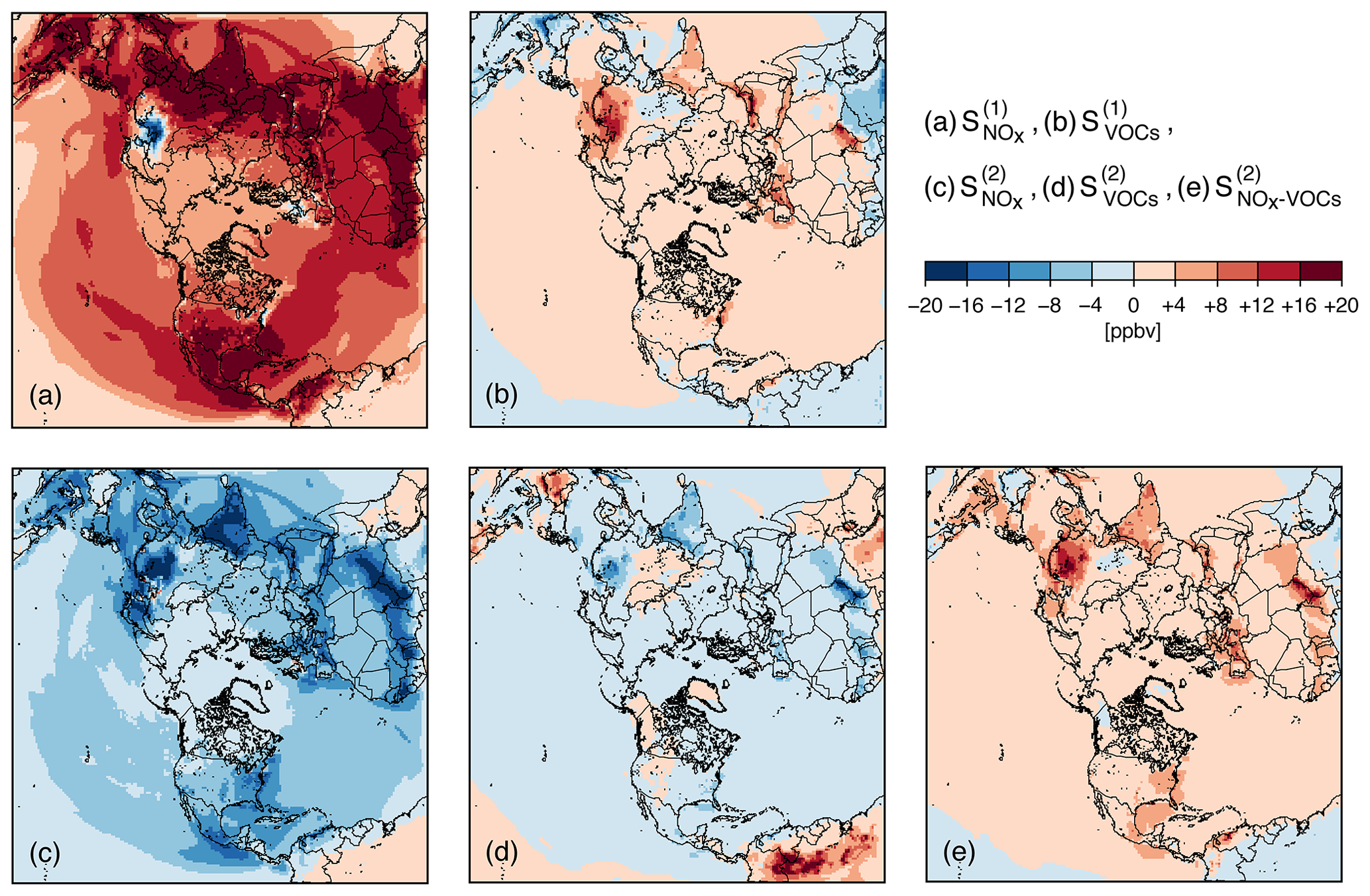
Figure 1Spatial distribution of the sensitivity coefficients of O3 to domain-wide emissions. (a) First-order sensitivity to NOx emissions, (b) first-order sensitivity to VOC emissions, panel (c) is the same as (a) but second order, panel (d) is the same as (b) but second order, and (e) second-order sensitivity to NOx and VOC emissions during April 2010. The sensitivity coefficients are monthly means computed from all hourly data on April 2010.
Determining the O3 sensitivity regime can provide useful information to policy makers designing emission reduction strategies by clarifying the relative importance of precursor emissions. Based on the relationships between the sensitivity coefficients, we determined O3-sensitivity regimes from threshold values revised from previous studies (Wang et al., 2011; Itahashi et al., 2013) as follows.
Grid cells meeting neither of these two criteria are considered to be in a transition regime. This classification is applied to all hourly HDDM results during April 2010 and then averaged. The O3-sensitivity regimes obtained through this analysis are shown in Fig. 2. The shading of NOx (purple) or VOC sensitive (green) indicates the high frequency of occurrence of sensitivity to NOx or VOC regime. As already suggested by the relative magnitudes of the sensitivity coefficients towards NOx and VOC emissions shown in Fig. 1, O3 during April 2010 is in a NOx-sensitive regime over the midlatitude Northern Hemisphere with the exception over the locations that had negative first-order sensitivity to NOx emission and were classified as VOC sensitive. Therefore, controls on NOx emissions can be an effective way to reduce surface O3 across almost the entire Northern Hemisphere but it may cause an increase of O3 mixing ratios over eastern China and some areas in Europe and the US. Due to the coarse grid resolution, H-CMAQ could partly missed the VOC-sensitive regime characterized over urban areas, and our previous study reported the dependency of photochemical indicators to judge the O3 regime (e.g., )) on model grid resolution (Zhang et al., 2009). Through the analysis of HDDM results for domain-wide emissions, this section provided an overview of O3 sensitivities and the response of O3 to precursor emissions over the Northern Hemisphere. The following section further investigates the sensitivity of surface O3 over the US by defining different emission source regions over the US and east Asia.
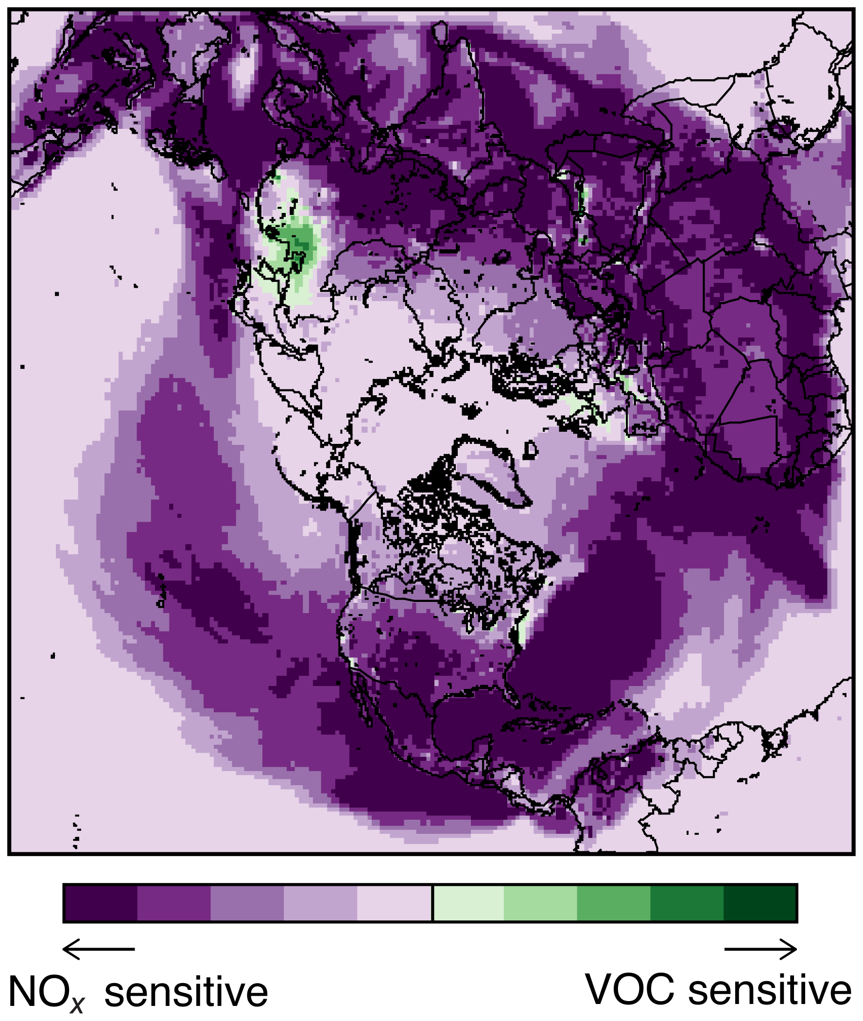
Figure 2Spatial distributions of the ozone-sensitive regime during April 2010.
4.2 Emission impacts from the US and east Asia at surface level
To investigate the emission impacts from the US and east Asia, we defined two source regions as shown in Fig. 3a. In this study, east Asia includes China, Taiwan, Mongolia, the Korean Peninsula (North and South Korea), and Japan. We conducted additional HDDM simulations using these two source regions and then calculated their sensitivity coefficients, which are shown in Figs. S2 and S3. The sensitivities from other regions except the US and east Asia are illustrated in Fig. S4. Based on these sensitivity coefficients, ZOCs of emissions from the US and east Asia are derived according to Eq. (5) and the resulting emission impacts are shown in Fig. 3b and c. The ZOCs of emissions from the US show more than 10 ppbv over the southeastern US and relatively small impacts around 2–8 ppbv in the western US. In some areas over the US that are characterized by a weak VOC-sensitive regime in Fig. 2 (e.g., Seattle, San Francisco, Los Angeles, around the Great Lakes, and New England regions), emissions from the US have small negative impacts. The US emission impacts extend to the Atlantic Ocean with impacts of more than 2 ppbv, which are comparable to those found over the western US, and then decrease over Africa. The ZOC of emissions from east Asia also shows positive impacts greater than 10 ppbv over China, Taiwan, Japan, and the western Pacific Ocean, with the exception of negative impacts over eastern China. These negative impacts indicate that the elimination of emissions can lead to O3 increase, because NO titration works to reduce the O3 mixing ratio over these areas, which have a high emission density. The analysis of the ZOC from east Asian emissions clearly illustrates the presence of trans-Pacific transport of O3. This transport on a monthly mean basis is estimated to be more than 2 ppbv over almost the entire Pacific Ocean and reaches many parts of North America, i.e., almost the entire US and Canada and western Mexico.
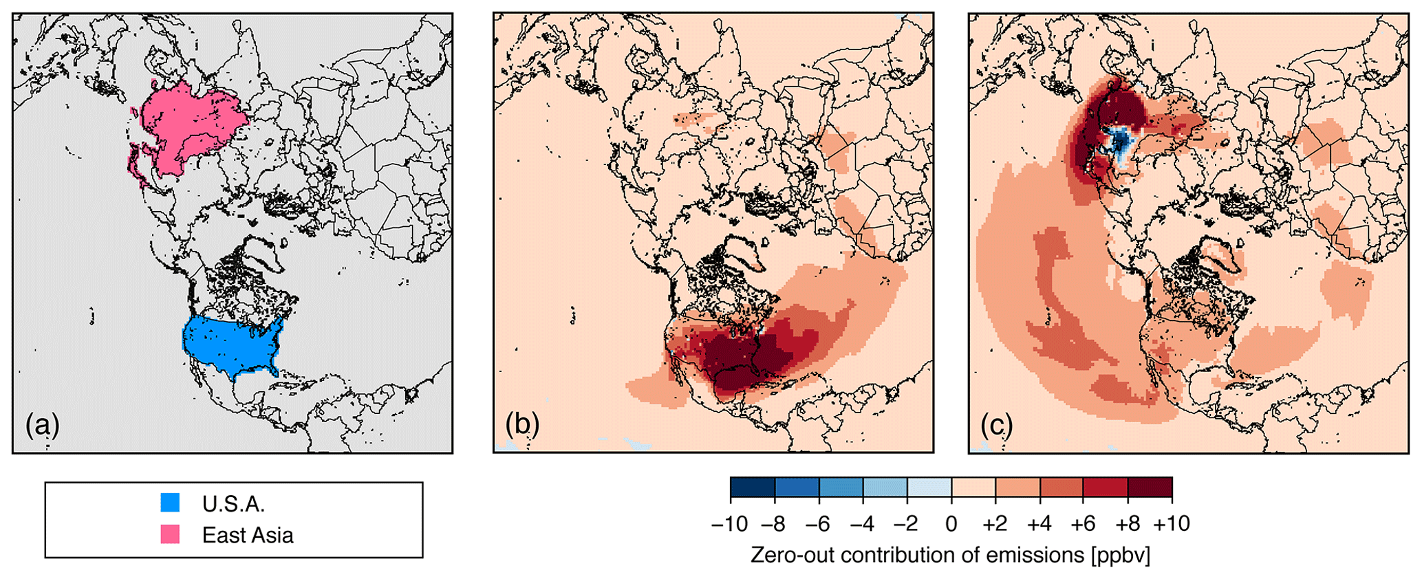
Figure 3(a) Source regions of the US and east Asia, and zero-out contribution of emissions from the (b) US and (c) east Asia during April 2010. East Asia is defined as China, Taiwan, Mongolia, the Republic of Korea, Democratic People's Republic of Korea, and Japan.
Detailed analyses of these impacts over the US are conducted by focusing on longitudinal differences. In this study, we use four time zones of Pacific, Mountain, Central, and Eastern Standard Time (abbreviated as PST, MST, CST, and EST, respectively) in the US and investigate O3 mixing ratio and ZOC of emission from the US and east Asia in these zones. Results for monthly and daily means are shown in Fig. 4. Consistent with previous studies (e.g., Simon et al., 2015), O3 mixing ratios have a longitudinal gradient with lower values in the west and higher values in the east (modeled monthly mean concentrations are 35.8, 39.3, 39.1, and 40.6 ppbv over PST, MST, CST, and EST, respectively). The results of the ZOC analysis reveal varying impacts from US and east Asian emissions across the four regions. For the US on a monthly mean domain-wide basis, the impact of domestic emissions surpasses that of east Asian emissions. Over the PST region, the monthly averaged impact of domestic emissions is 3.2 ppbv, while that of east Asian emissions is 2.8 ppbv; i.e., the impacts from both source regions over the PST zone are comparable. It should be noted that the daily averaged impact of east Asian emissions can exceed that of US emissions on some days (e.g., in early April and during 27–30 April), suggesting the significant role of episodic trans-Pacific transport on air quality over the western US. In contrast to the situation over the PST zone, the impact from domestic emissions always clearly exceeds the impact from east Asian emissions in the MST, CST, and EST zones; this feature strengthens towards the east. For example, the temporal variations of daily averaged O3 mixing ratios and the impacts of domestic emissions are well correlated over the EST zone. The impact of east Asian emissions is small compared to that of US emissions over the CST and EST zones, but it is not negligible. These impacts are 2.1 ppbv on a monthly average basis (ranging between 1.2 and 3.0 ppbv on a daily basis) over CST and 1.9 ppbv on a monthly average basis (ranging between 1.2 and 2.8 ppbv on a daily basis) over EST through April 2010.
Table 1Summary of the correlation between modeled MD8O3 and the zero-out contribution of emissions from the US and east Asia.
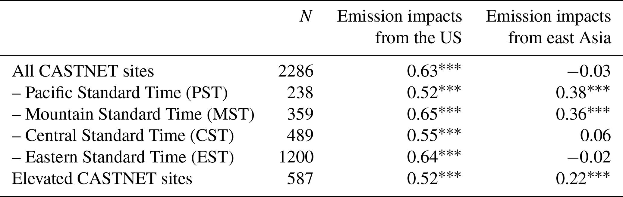
Note: significance levels by Student's t test for correlation coefficients between observations and simulations are marked as *p < 0.05, , and , and lack of a mark indicates no significance.
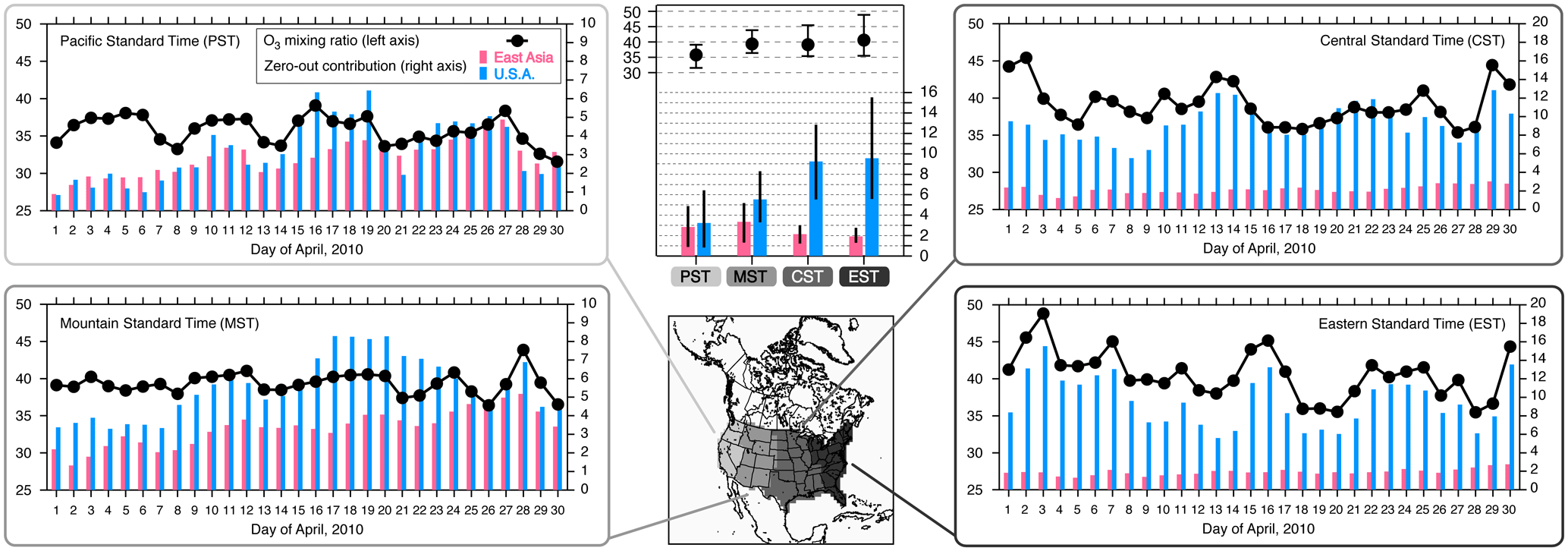
Figure 4Daily and monthly averaged O3 mixing ratio (left axis; black circles and thick lines) and zero-out contribution from the US and east Asia (right axis; light blue and light red bars, respectively) summarized over four time zones of Pacific, Mountain, Central, and Eastern Standard Time (PST, MST, CST, and EST) in the US. The units of the left and right axes are ppbv. On a monthly average basis (center panel), whiskers indicates daily minimum and maximum. Note that the axis of zero-out contributions is different in the left (PST and MST) and right panels (CST and EST).
To illuminate the relationship between surface O3 mixing ratio and impacts from US and east Asian emissions, in Fig. 5, scatter plots were constructed using model-derived estimates at all CASTNET sites and at elevated CASTNET sites only (refer to Fig. 10 of Itahashi et al., 2020). The statistical analysis of R and its significance level by Student's t test between surface O3 mixing ratio and these impacts by emissions is listed in Table 1. At all CASTNET sites, the relationship between the modeled MD8O3 and the impact of emissions from the US shows a positive slope with R of 0.63 and p < 0.001, confirming that domestic emissions are generally the cause of high surface O3 mixing ratios. On the other hand, the relationship between modeled MD8O3 and the impact of emissions from east Asia is flat, with R of −0.03 and no significance, suggesting that constant impacts are found in the US but do not directly relate to high surface O3 mixing ratios. A noticeable result is that the relationship varies across the regions. Each point in the scatter plots is shaded by time zone, and it can be seen that high O3 mixing ratios over the CST and EST zones (darker black in Fig. 5c) are not linked to the impacts of east Asian emissions (R of 0.06 and −0.03, respectively, and not significant), while moderately higher O3 mixing ratios found over PST and MST (lighter black in Fig. 5c) appear to be linked to higher impacts from east Asian emissions (R values were 0.36 and 0.36, respectively, and p < 0.001). These analyses are repeated using data from sites with an elevation higher than 1000 m (see Table S1 in the Supplement). At this subset of stations, the O3 mixing ratio shows a positive relationship with emissions from both the US (R of 0.52 with p < 0.001) and east Asia (R of 0.22 with p < 0.001). This might be partly because most of the elevated CASTNET sites are located in the western US (17 of 21 elevated sites are located in the PST or MST zones). Since long-range transport occurs aloft and since changes in pollutant concentrations influence their ground-level values (e.g., Mathur et al., 2018b), in the next section, we specifically investigate the impacts of emissions from different source regions on O3 aloft.

Figure 5Relationship between modeled MD8O3 at the surface and zero-out contribution of emissions from (a, b) the US and (c, d) east Asia. The points are shaded by four time zones in the US: (a, c) all CASTNET sites and (b, d) elevated CASTNET sites defined as having an elevation greater than 1000 m (see also Table S1).
4.3 Emission impacts on O3 aloft
In this section, we focus on the impacts of US and east Asian emissions on O3 distributions through the troposphere over the US. Monthly averaged O3 mixing ratios and ZOCs of emissions from the US and east Asia at different altitudes in the free troposphere are shown in Fig. 6. As the reference, monthly averaged ZOCs of domain-wide emissions at different altitudes at surface and in the free troposphere are shown in Fig. S5. Throughout this study, we define the free troposphere as ranging from 750 to 250 hPa and refer to pressure levels of 750, 500, and 250 hPa as the bottom, middle, and top of the free troposphere, respectively. The results of this analysis are also summarized in Table 2. O3 mixing ratios are larger over continents from the surface to 750 hPa (i.e., boundary layer) but are more dispersed over midlatitudes to high latitudes at 500 and 250 hPa (Fig. 6). O3 mixing ratios at the surface exhibit a longitudinal gradient with lower values over the western US and higher values over the eastern US, and the same gradient is seen at 750 hPa. However, there are no longitudinal gradients at 500 hPa with 54 ppbv over the entire US, and a reversed longitudinal gradient with western highs and eastern lows is found at 250 hPa (Table 2).
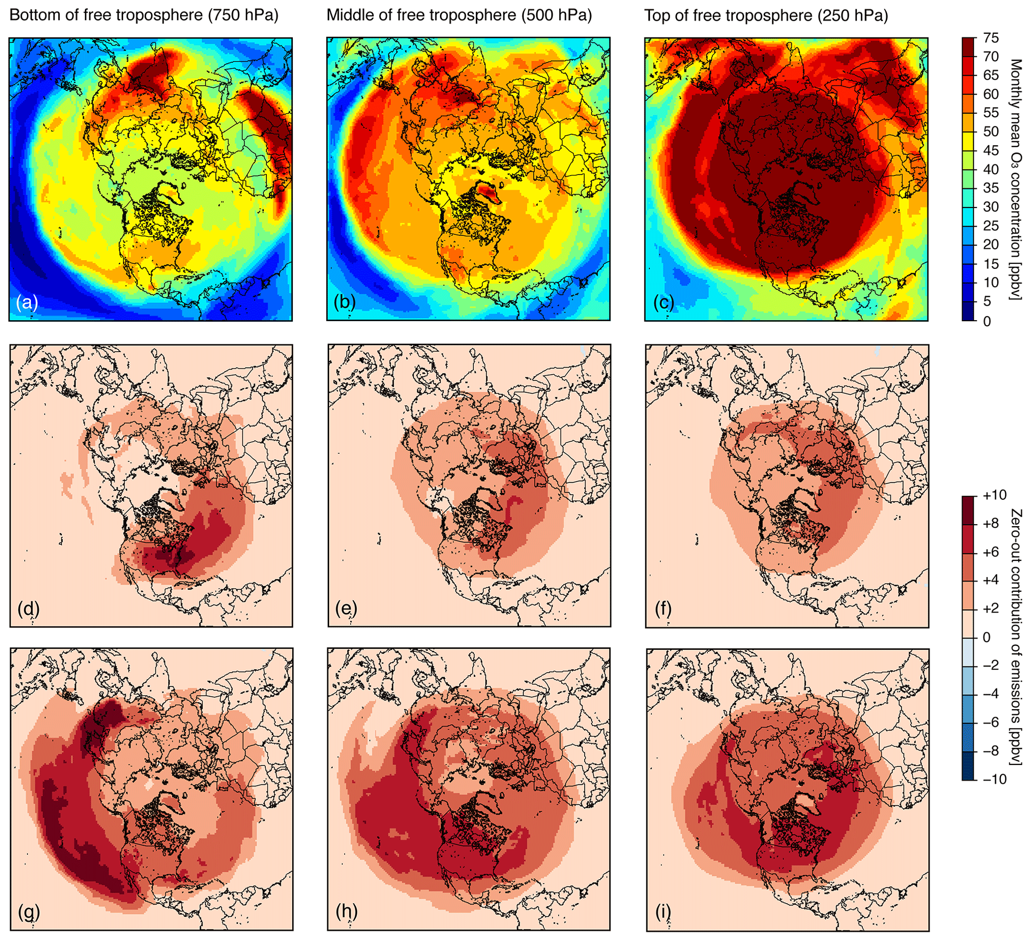
Figure 6Monthly averaged (a–c) O3 concentration and zero-out contribution from the (d–f) US and east (g–i) Asia at the bottom of free troposphere (750 hPa; a, d, g), middle of free troposphere (500 hPa; b, e, h), and top of free troposphere (250 hPa; c, f, i).
Table 2Summary of O3 concentration and zero-out contribution of emissions from the US and east Asia, and sensitivity of O3VORT over four time zones in the US during April 2010.
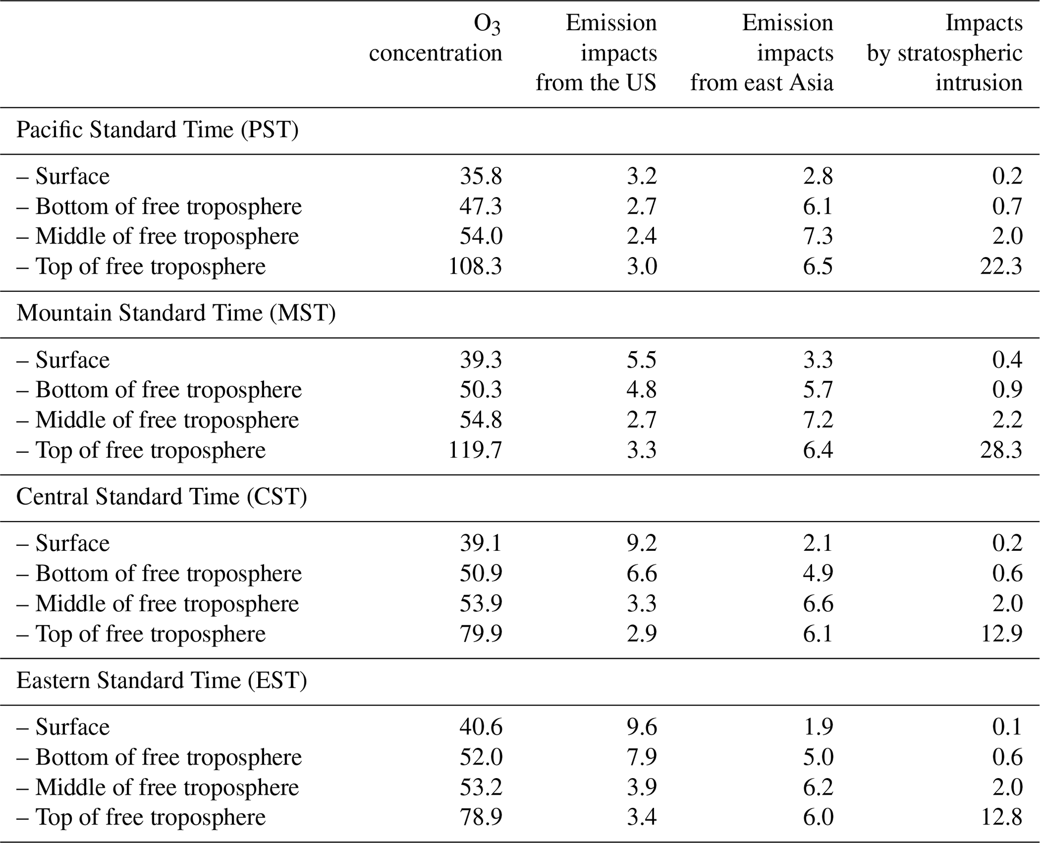
Note: all units are ppbv.
Once O3 is lofted to free troposphere, its sinks are not effective, and consequently it can be transported further. For ZOC of US emissions, the largest contribution is found over the southeast US at 750 hPa but the impacts of US emissions stretch far across the Atlantic to Europe, north Africa, Eurasia, and even Japan with values above 2 ppbv. Areas where the impact of US emissions exceeds 2 ppbv are shown over the entire Northern Hemisphere at 500 and 250 hPa (Fig. 6). It should also be noted that the impacts of US emissions on the US remained constant or declined with increasing altitude. In particular, constant impacts from US emissions with increasing altitude are found over the PST zone, whereas decreasing impacts are found over the MST, CST, and EST zones. From the middle to the top of the free troposphere, the impacts of US emissions on the US are around 2–3 ppbv (Table 2). For ZOC of east Asian emissions, extended impacts on the US when increasing altitude are shown (Fig. 6). At 750 hPa, the impacts are found over the entire Pacific Ocean with more than 10 ppbv around Hawaii and contribution as high as 4–8 ppbv over the entire US. At 500 hPa, its impacts are smaller over the Pacific Ocean with less than 8 ppbv; however, the impacts are above 6 ppbv almost across the entire US, surpassing the impacts found at 750 hPa. At 250 hPa, the impacts are slightly decreased beyond the US but stretch across a broader range to Europe and western Russia (Fig. 6). It is shown that the impacts of east Asian emissions are around 5 ppbv or more over the entire free troposphere over the US (Table 2). From the middle to the top of the free troposphere, the impacts of emissions from east Asia are twice or more those of US emissions over the eastern and western US, respectively.
In characterizing the dominant sources of O3 aloft, the role of stratospheric air masses also needs to be considered. In our Part 1 paper, we developed an air mass characterization technique, but it was limited to estimate the air mass burden on column O3. In this Part 2 paper, to unify the methodology investigating sensitivities to model parameters, the sensitivity towards O3 specification near the tropopause based on a potential vorticity scaling, hereafter referred to as O3VORT, is directly calculated. The results of the O3 sensitivity towards O3VORT are shown in Fig. 7 at the surface, 750, 500, and 250 hPa with different color scales. Not surprisingly, the sensitivity of O3 to O3VORT shows increasing values with increasing altitude. At the surface level and on a monthly averaged timescale, the impact of STT is less than 1 ppbv, except over the Tibetan Plateau because of its elevation. In other regions, smaller impacts of STT are noted over the western US and north Africa; the former is due to the high elevation of the Rocky Mountains, whereas the latter may be related to active convection. Impacts of STT exceeding 1 ppbv are found over midlatitudes areas at 750 hPa, and stronger impacts exceeding 5 ppbv are found at 500 hPa. At 250 hPa, the impacts of STT are shifted towards high latitudes and exceed 25 ppbv, reflective of the lower tropopause height at higher latitudes (Fig. 7). Over the US, the monthly averaged impacts of STT are below 1 ppbv at the surface and 750 hPa and increase from around 2 ppbv at 500 hPa to more than 10 ppbv at 250 hPa (Table 2). At 250 hPa, the impacts of STT range from more than 20 ppbv in the west and a low of around 10 ppbv in the east; therefore, these differences partly account for the longitudinal gradient of the O3 mixing ratio modeled at the top of free troposphere.

Figure 7Monthly averaged sensitivity of O3VORT at (a) surface, (b) bottom of free troposphere (750 hPa), (c) middle of free troposphere (500 hPa), and (d) top of free troposphere (250 hPa).
Note that O3 concentration fields and the sum of sensitivities do not generally equal each other because of nonlinearities in O3 formation. Moreover, the zero-out contributions for US and east Asian emissions represent only a portion of the total emissions burden, and the emissions' sensitivity calculations can also be affected by initial and boundary conditions. To investigate this further, the temporal evolution of O3 concentrations and sensitivities towards O3VORT, O3IC, O3BC, and domain-wide emissions' ZOC are presented in Figs. S6–S9. The figures show time series of these contributions averaged over the PST, MST, CST, and EST areas in the US at the surface, 750, 500, and 250 hPa, corresponding to the results presented in Table 2. These figures show that the domain-wide emission zero-out contributions (Fig. S5) are larger than those of zero-out contributions from the US and east Asia (Fig. 6 and Table 2), pointing to the impact of emissions from other regions on simulated ozone concentrations. As expected, the impact of O3BC is small over the US due to the distance from the equatorial boundaries. At the beginning of the simulation, O3 concentrations are dominated by initial conditions, as shown by the close agreement between the O3 concentration and O3IC curves during the first half of March. The sensitivity towards O3IC declines throughout the simulation, while O3VORT and ZOC increase and begin to dominate the O3 variation by April. However, even after the 1-month spin-up period, O3IC is still present over all time zones and all altitudes. In this study, we initiated the H-CMAQ simulation from the prior model simulation for 2010 (Hogrefe et al., 2018); however, this result suggest that spin-up periods longer than 1 month may be necessary to fully capture the effects of emissions and O3VORT contributions through calculating HDDM sensitivities over a hemispheric-scale modeling domain. Finally, Figs. S6–S9 still show differences between simulated concentrations and the sum of O3VORT, O3IC, O3BC, and ZOC. Aside from the nonlinearities and interactions mentioned above, this likely is also caused by contributions of initial conditions of species other than O3 (e.g., PAN or N2O5) to the simulated O3 levels.
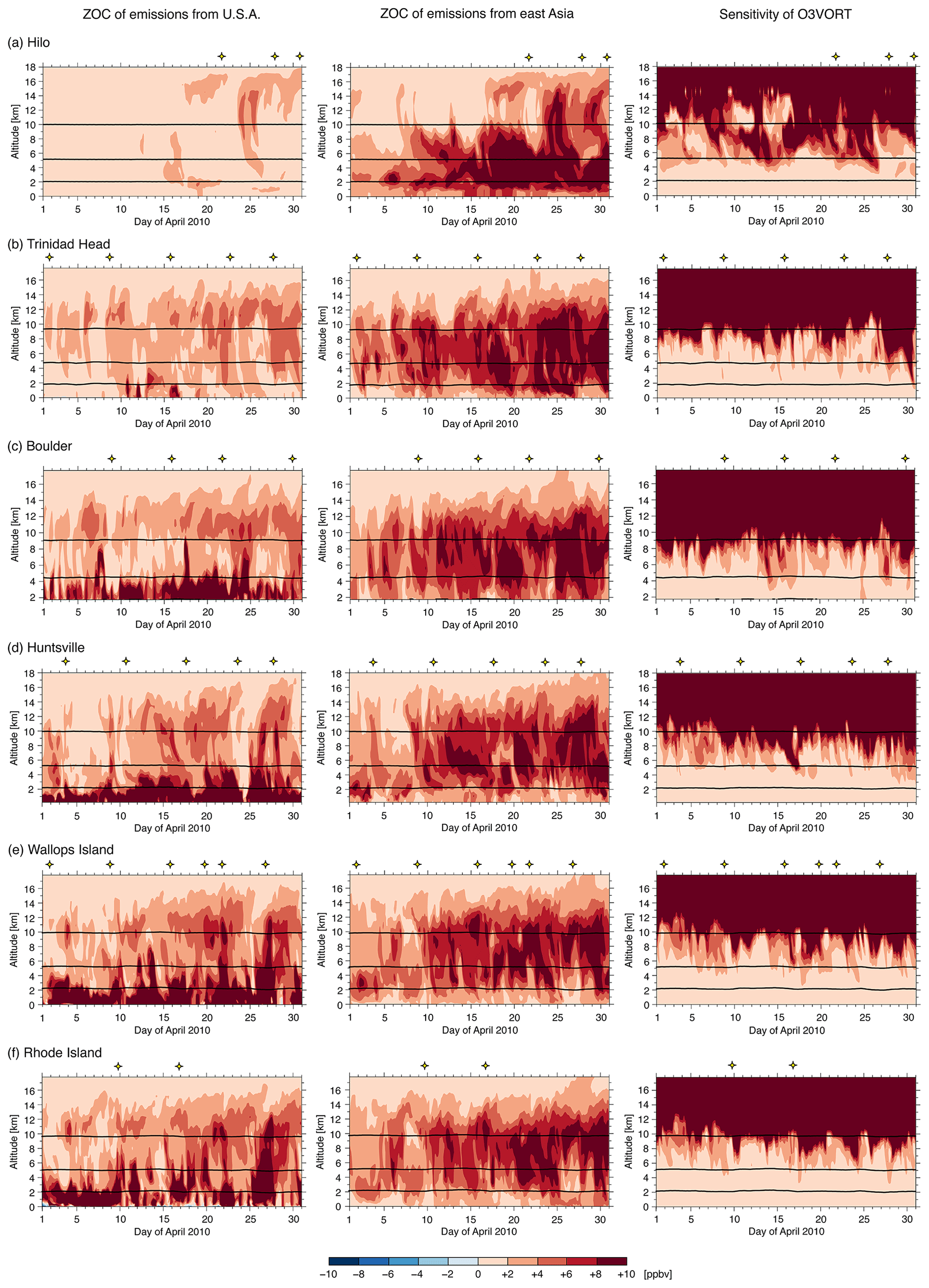
Figure 8Curtain plots of (left) ZOC of emissions from the US, (center) ZOC of emissions from east Asia, and (right) sensitivity of O3VORT at US ozonesonde sites of (a) Hilo (HI), (b) Trinidad Head (CA), (c) Boulder (CO), (d) Huntsville (AL), (e) Wallops Island (VA), and (f) Rhode Island during April 2010. Yellow stars indicate the time of available ozonesonde measurements. Thick lines from bottom to top indicate 750, 500, and 250 hPa as a representative bottom, middle, and top of free troposphere.
To illustrate altitude dependencies of the impacts of US and east Asian emission and STT, vertical cross sections (“curtain plots”) of these impacts at six ozonesonde sites across the US are examined in Fig. 8 (refer to Figs. 4 and S5 of Itahashi et al., 2020). In these curtain plots, the pressure levels of 750, 500, and 250 hPa are marked to indicate the representative altitude of the bottom, middle, and top of the free troposphere. The comparison of the ZOCs from US and east Asian emissions clearly shows the differences of their vertical structures. Over these ozonesonde sites, except Hilo (Fig. 8a), the emission impacts from the US greater than 10 ppbv are mostly confined to below 750 hPa (within the boundary layer) and occasionally extend into the free troposphere. In contrast, the emission impacts from east Asia can predominantly be found in the free troposphere and sometimes extend into the boundary layer (below 750 hPa) and/or the upper model layers (above 250 hPa). These patterns further confirm that pollution lofted to the free troposphere over Asia can undergo efficient transport across the Pacific and entrain to the lower troposphere and boundary layer over the US. The sensitivity towards O3VORT is the dominant factor over the upper model layers (above 250 hPa) and downward into the upper part of the free troposphere, but most of its episodic impact does not reach the middle of the free troposphere (500 hPa) or below. The strong STT events seen in these cross sections, i.e., the events in early and late April at Trinidad Head (Fig. 8b), early April at Boulder (Fig. 8c), late April at Huntsville (Fig. 8d), and mid-April at Wallops Island (Fig. 8e) and Rhode Island (Fig. 8f), are generally consistent with the results inferred from the air mass classification technique presented in the Part 1 paper. It should be however noted that a more robust quantification of the fraction of ground-level O3 that originated in the stratosphere and its seasonal and spatial distributions would require conduct of longer-term sensitivity simulations than those examined here.
4.4 Perspective on the changes in trans-Pacific transport
As has been shown in previous studies and affirmed in the current work, trans-Pacific transport can impact air quality in the US. April 2010 was used as the target period for our analysis because El Niño conditions during that time period favored trans-Pacific transport. In this section, we estimate the variation of trans-Pacific transport caused by recent emission changes. According to the NOAA Climate Prediction Center (CPC), strong and long-lasting El Niño conditions occurred from late 2014 to the middle of 2016 (NOAA and CPC, 2018). Observed average MD8O3 over the US was 46.9 ppbv in April 2015, a decline from its April 2010 values of 52.2 ppbv, and the number of sites exceeding the NAAQS declined from 39 sites in April 2010 to 7 sites in April 2015. From 2010 to 2015, annual NOx (VOC) emissions in the US decreased from 13.4 (13.6) Tg to 10.6 (12.9) Tg (see Fig. S1 of Itahashi et al., 2020). These emission reductions likely contributed to the decline of the observed O3 mixing ratios relative to the 2010 values. How about the trans-Pacific transport? Anthropogenic emissions in China grew during the 2000s (Itahashi et al., 2014) and reached the highest levels in the world in 2010; however, substantial reductions have been measured by satellites since then (Irie et al., 2016; Krotkov et al., 2016; van der A et al., 2017; Itahashi et al., 2018). In addition, bottom-up emission inventories indicate that Chinese NOx emissions were reduced as a consequence of clean air actions (Zheng et al., 2018). In particular, Zheng et al. (2018) report that annual NOx emissions were reduced from 26.5 Tg in 2010 to 23.7 Tg in 2015, while annual VOC emissions increased from 25.9 Tg in 2010 to 28.5 Tg in 2015. While NOx emissions have been regulated and subsequently declined after reaching a peak of 29.2 Tg in 2012, the situation is more complex for VOC emissions which show decreases from the residential and transportation sectors but increases from the industrial sector and solvent use. Applying the percentage changes in Chinese emissions from 2010 to 2015 to the HDDM sensitivities for east Asian emissions (assuming that changes in east Asian emissions are dominated by changes in China), we estimated their impacts on tropospheric O3 mixing ratios.
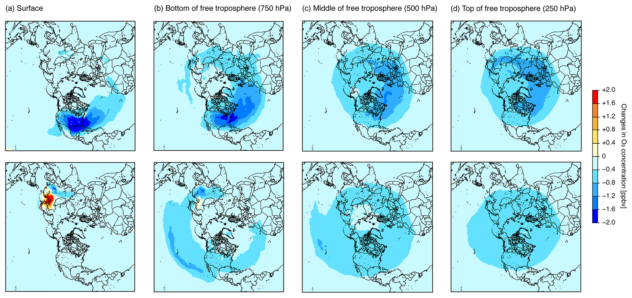
Figure 9Perspective of changes in O3 concentration resulting from estimated 2010–2015 emission changes over (top panels) the US and (bottom panels) east Asia at the (a) surface, (b) bottom of free troposphere (750 hPa), (c) middle of free troposphere (500 hPa), and (d) top of free troposphere (250 hPa).
The changes in O3 mixing ratio caused by emission changes between 2010 and 2015 over the US and east Asia can be investigated via Eq. (4). Based on the emission changes noted above, the resulting values of εi and εj in Eq. (4) are −20.9 % and −5.1 % for NOx and VOC emissions from the US, and −10.6 % and 10.0 % for NOx and VOC emissions from east Asia, respectively. The estimated spatial changes in O3 mixing ratios at the surface and aloft are shown in Fig. 9, and estimates for monthly and daily means over four time zones in the US are shown in Fig. 10 in a similar manner to Fig. 4. The US emission reductions between 2010 and 2015 resulted in generally reducing surface O3 mixing ratios with changes of at least −0.5 ppbv across the entire US and up to −5.0 ppbv over the southeast US. Exceptions are found over Seattle, San Francisco, Los Angeles, around the Great Lakes, and in New England regions that were characterized as VOC sensitive in Sect. 3.2. These changes are expected because reductions in NOx emission were greater than those in VOC emissions across the US. It is also shown that the US emission reductions cause a reduction of O3 mixing ratio over the free troposphere. On the time-zone-averaged basis, the changes in monthly mean O3 mixing ratios are −0.5, −1.1, −1.8, and −1.5 ppbv over PST, MST, CST, and EST, respectively (Fig. 10). The maximum reductions are found over CST because EST contains the complex sensitivity over New England regions. In contrast, the changes in east Asian emissions between 2010 and 2015 do not cause a noticeable reduction in surface O3 mixing ratios over the US, while they led to O3 mixing ratio increases of more than 1 ppbv over eastern China, the Korean Peninsula, and some parts of Japan on a monthly average basis (Fig. 9). These increases are expected both because these areas were shown to be VOC sensitive in Sect. 3.2 and because of the increase in VOC emissions. On a time-zone-averaged basis, changes in east Asian emissions between 2010 and 2015 are estimated to change the monthly mean O3 mixing ratio across the US by about −0.1 to −0.3 ppbv. The corresponding changes in daily average surface-level O3 mixing ratio were also less than −0.5 ppbv (Fig. 10). A slight reduction in monthly mean O3 mixing ratios of around −0.5 ppbv was estimated across large parts of the Northern Hemisphere free troposphere, indicating that the reductions in east Asian emissions that occurred between 2010 and 2015 can partly contribute to a weakening of trans-Pacific O3 transport over the free troposphere. However, the reductions in Asian emissions during 2010 and 2015 did not appear to alter the monthly mean surface-level O3 mixing ratio across the US.

Figure 10Perspective of daily and monthly averaged changes in O3 mixing ratio resulting from estimated 2010–2015 emission changes over the US (light blue bars) and east Asia (light red bars) summarized over four time zones of Pacific, Mountain, Central, and Eastern Standard Time (PST, MST, CST, and EST) in the US. The units are ppbv. On a monthly average (center panel), whiskers indicate daily minimum and maximum. Note that the axis is different in the left (PST and MST) and right panels (CST and EST).
In this study, the regional chemical transport model extended for hemispheric applications, H-CMAQ, is applied to investigate trans-Pacific transport during April 2010. The previous paper (Part 1) demonstrated that STT can cause impacts on tropospheric O3 but did not relate to the enhancement of surface O3 mixing ratios. Therefore, in this Part 2 paper, emission impacts are investigated based on the sensitivity analysis through HDDM. The sensitivities to domain-wide emissions indicate NOx-sensitive conditions during April 2010 for tropospheric O3 across most of the Northern Hemisphere except over eastern China and a few urban areas over the US and Europe. Contributions of emissions from source regions covering the US and east Asia were examined through propagation of emission sensitivities in H-CMAQ. Analyses of estimated zero-out contributions from the computed sensitivities demonstrate comparable impacts of US and east Asian emissions on surface-level O3 over the western US during April 2010, whereas contributions from US emissions dominate O3 distributions over the eastern US. The analyses also reveal the significant impacts of east Asian emissions on free tropospheric O3 over the US which surpass the estimated impacts of US emissions, further confirming the long-range pollution transport conceptual view wherein pollution from source regions is convectively lofted to the free troposphere and efficiently transported intercontinentally. Finally, the effects of recent emission changes on the trans-Pacific transport of O3 are estimated. Under the assumed similar meteorological conditions in 2010 and 2015, it can be concluded that trans-Pacific transport resulting from emission changes did not lead to significant changes in O3 mixing ratio over the US at the surface level even on a daily mean basis in April. The year 2015 was selected because of El Niño conditions favorable to trans-Pacific transport; however, the impacts of changes in year-specific meteorological conditions are not investigated here. The possible impacts of changing climate on trans-Pacific transport (e.g., Glotfelty et al., 2014) should however be further examined. Long-term trend analysis taking into account both emission and meteorological changes (e.g., Mathur et al., 2018a) will be conducted in future work to further understand variability in trans-Pacific transport patterns and contributions. While the 1-month simulation period and analysis of a representative springtime month helped characterize aspects of trans-Pacific transport, longer-term simulations need to be conducted to further quantify the seasonal source region contributions to trans-Pacific transport. The results presented here are based on monthly or daily mean ozone during April 2010 and are not expected to be consistent with other metrics (e.g., MD8O3) not analyzed here or times of the year when transport is less favorable and local ozone production is more favorable. The longer-term calculations will also help better quantify the STT contributions to surface-level O3 which appear to be lower in the current analysis relative to previous studies (e.g., Lelieveld and Dentener, 2000; Lin et al., 2015; Mathur et al., 2017).
Source code for version 5.2 of the CMAQ model can be downloaded from https://github.com/USEPA/CMAQ/tree/5.2 (U.S. EPA and ORD, 2017a, b). For further information, please visit the US Environmental Protection Agency website for the CMAQ system: https://www.epa.gov/cmaq (U.S. EPA, 2020).
The supplement related to this article is available online at: https://doi.org/10.5194/acp-20-3397-2020-supplement.
SI performed the analysis of observation and model simulation, and prepared the manuscript with contributions from all co-authors. RM and CH contributed to establishing the hemispheric modeling application for this study and prepared the emission dataset and initial condition from previous long-term simulation results. SLN contributed to the discussion of sensitivity analysis based on the higher-order decoupled direct method. YZ contributed to the literature review of trans-Pacific transport and refined this research through simulation designs and results' interpretation.
The authors declare that they have no conflict of interest.
The views expressed in this paper are those of the authors and do not necessarily reflects the views or policies of the US Environmental Protection Agency.
Yang Zhang acknowledges support from the 2017–2018 NC State Internationalization Seed Grant and the 2019–2020 NC State Kelly Memorial Fund for US-Japan Scientific Cooperation.
This paper was edited by Robert Harley and reviewed by two anonymous referees.
Acid Deposition Monitoring Network in East Asia (EANET): available at: http://www.eanet.asia, last access: 19 April 2018.
Appel, K. W., Napelenok, S. L., Foley, K. M., Pye, H. O. T., Hogrefe, C., Luecken, D. J., Bash, J. O., Roselle, S. J., Pleim, J. E., Foroutan, H., Hutzell, W. T., Pouliot, G. A., Sarwar, G., Fahey, K. M., Gantt, B., Gilliam, R. C., Heath, N. K., Kang, D., Mathur, R., Schwede, D. B., Spero, T. L., Wong, D. C., and Young, J. O.: Description and evaluation of the Community Multiscale Air Quality (CMAQ) modeling system version 5.1, Geosci. Model Dev., 10, 1703–1732, https://doi.org/10.5194/gmd-10-1703-2017, 2017.
Clappier, A., Belis, C. A., Pernigotti, D., and Thunis, P.: Source apportionment and sensitivity analysis: two methodologies with two different purposes, Geosci. Model Dev., 10, 4245–4256, https://doi.org/10.5194/gmd-10-4245-2017, 2017.
Clean Air Status and Trends Network (CASTNET), U.S. Environmental Protection Agency Clean Air Markets Division: available at: https://www.epa.gov/castnet, last access: 26 April 2018.
Cohan, D. S., Hakami, A., Hu, Y. T., and Russell, A. G.: Nonlinear response of ozone to emissions: Source apportionment and sensitivity analysis, Environ. Sci. Technol., 39, 6739–6748, https://doi.org/10.1021/es048664m, 2005.
Emery, C., Liu, Z., Russell, A. G., Odman, M. T., Yarwood, G., and Kumar, N.: Recommendations on statistics and benchmarks to assess photochemical model performance, J. Air Waste Manage., 67, 582–598, https://doi.org/10.1080/10962247.2016.1265027, 2017.
Fiore, A., Jacob, D. J., Liu, H., Yantosca, R. M., Fairlie, T. D., and Li, Q.: Varaiability in surface ozone background over the United States: Implications for air quality policy, J. Geophys. Res., 108, 4787, https://doi.org/10.1029/2003JD003855, 2003.
Fiore, A. M., Jacob, D. J., Bey, I., Yantosca, R. M., Field, B. D., Fusco, A. C., and Wilkinson, J. G.: Background ozone over the United States in summer: Origin, trend, and contribution to pollution episodes, J. Geophys. Res., 107, 4275, https://doi.org/10.1029/2001JD000982, 2002.
Galmarini, S., Koffi, B., Solazzo, E., Keating, T., Hogrefe, C., Schulz, M., Benedictow, A., Griesfeller, J. J., Janssens-Maenhout, G., Carmichael, G., Fu, J., and Dentener, F.: Technical note: Coordination and harmonization of the multi-scale, multi-model activities HTAP2, AQMEII3, and MICS-Asia3: simulations, emission inventories, boundary conditions, and model output formats, Atmos. Chem. Phys., 17, 1543–1555, https://doi.org/10.5194/acp-17-1543-2017, 2017.
Glotfelty, T., Zhang, Y., Karamchandani, P., and Streets, D. G.: Will the role of intercontinental transport change in a changing climate?, Atmos. Chem. Phys., 14, 9379–9402, https://doi.org/10.5194/acp-14-9379-2014, 2014.
Guo, J. J., Fiore, A. M., Murray, L. T., Jaffe, D. A., Schnell, J. L., Moore, C. T., and Milly, G. P.: Average versus high surface ozone levels over the continental USA: model bias, background influences, and interannual variability, Atmos. Chem. Phys., 18, 12123–12140, https://doi.org/10.5194/acp-18-12123-2018, 2018.
Haagen-Smit, A. J. and Fox, M. M.: Photochemical Ozone Formation with Hydrocarbons and Automobile Exhaust, Air Repair, 4, 105–136, https://doi.org/10.1080/00966665.1954.10467649, 1954.
Hakami, A., Odman, M. T., and Russell, A. G.: High-order, direct sensitivity analysis of multidimensional air quality models, Environ. Sci. Technol., 37, 2442–2452, https://doi.org/10.1021/es020677h, 2003.
Hakami, A., Odman, M. T., and Russell, A. G.: Nonlinearity in atmospheric response: A direct sensitivity analysis approach, J. Geophys. Res., 109, D15303, https://doi.org/10.1029/2003JD004502, 2004.
Hogrefe, C., Liu, P., Pouliot, G., Mathur, R., Roselle, S., Flemming, J., Lin, M., and Park, R. J.: Impacts of different characterizations of large-scale background on simulated regional-scale ozone over the continental United States, Atmos. Chem. Phys., 18, 3839–3864, https://doi.org/10.5194/acp-18-3839-2018, 2018.
Hoskins, B. J., McIntyre., M. E., and Robertson, A. W.: On the use and significance of isentropic potential vorticity maps, Q. J. Roy. Meteor. Soc., 111, 877–946, 1985.
Huang, M., Carmichael, G. R., Pierce, R. B., Jo, D. S., Park, R. J., Flemming, J., Emmons, L. K., Bowman, K. W., Henze, D. K., Davila, Y., Sudo, K., Jonson, J. E., Tronstad Lund, M., Janssens-Maenhout, G., Dentener, F. J., Keating, T. J., Oetjen, H., and Payne, V. H.: Impact of intercontinental pollution transport on North American ozone air pollution: an HTAP phase 2 multi-model study, Atmos. Chem. Phys., 17, 5721–5750, https://doi.org/10.5194/acp-17-5721-2017, 2017.
Itahashi, S., Uno, I., and Kim, S-T.: Seasonal source contributions of tropospheric ozone over East Asia based on CMAQ-HDDM, Atmos. Environ., 70, 204–217, https://doi.org/10.1016/j.atmosenv.2013.01.026, 2013.
Itahashi, S., Uno, I., Irie, H., Kurokawa, J.-I., and Ohara, T.: Regional modeling of tropospheric NO2 vertical column density over East Asia during the period 2000–2010: comparison with multisatellite observations, Atmos. Chem. Phys., 14, 3623–3635, https://doi.org/10.5194/acp-14-3623-2014, 2014.
Itahashi, S., Hayami, H., and Uno, I.: Comprehensive study of emission source contributions for tropospheric ozone formation over East Asia, J. Geophys. Res., 120, 331–358, https://doi.org/10.1002/2014JD022117, 2015.
Itahashi, S., Yumimoto, K., Uno, I., Hayami, H., Fujita, S.-I., Pan, Y., and Wang, Y.: A 15-year record (2001–2015) of the ratio of nitrate to non-sea-salt sulfate in precipitation over East Asia, Atmos. Chem. Phys., 18, 2835–2852, https://doi.org/10.5194/acp-18-2835-2018, 2018.
Itahashi, S., Mathur, R., Hogrefe, C., and Zhang, Y.: Modeling stratospheric intrusion and trans-Pacific transport on tropospheric ozone using hemispheric CMAQ during April 2010 – Part 1: Model evaluation and air mass characterization for stratosphere–troposphere transport, Atmos. Chem. Phys., 20, 3373–3396, https://doi.org/10.5194/acp-20-3373-2020, 2020.
Irie, H., Muto, T., Itahashi, S., Kurokawa, J., and Uno, I.: Turnaround of tropospheric nitrogen dioxide pollution trends in China, Japan, and South Korea, SOLA, 12, 170–174, https://doi.org/10.2151/sola.2016-035, 2016.
Jacob, D. J., Logan, J. A., and Murti, P.: Effect of rising Asia emissions on surface ozone in the United States, Geophys. Res. Lett., 26, 2175–2178, 1999.
Jaffe, D. A., Cooper, O. R., Fiore, A. M., Henderson, B. H., Tonnesen, G. S., Russell, A. G., Henze, D. K., Langford, A. O., Lin, M., and Moore, T.: Scientific assessment of background ozone over the U.S.: Implications for air quality management, Elem. Sci., Anth., 6, 56, https://doi.org/10.1525/elementa.309, 2018.
Kim, S.-T., Byun, D. W., and Cohan, D. S.: Contribution of inter- and intra-state emissions to ozone over Dallas-Fort Worth, Texas, Civil Eng. Environ. Syst., 26, 103–116, 2009.
Krotkov, N. A., McLinden, C. A., Li, C., Lamsal, L. N., Celarier, E. A., Marchenko, S. V., Swartz, W. H., Bucsela, E. J., Joiner, J., Duncan, B. N., Boersma, K. F., Veefkind, J. P., Levelt, P. F., Fioletov, V. E., Dickerson, R. R., He, H., Lu, Z., and Streets, D. G.: Aura OMI observations of regional SO2 and NO2 pollution changes from 2005 to 2015, Atmos. Chem. Phys., 16, 4605–4629, https://doi.org/10.5194/acp-16-4605-2016, 2016.
Lelieveld, J. and Dentener, F. J.: What controls tropospheric ozone?, J. Geophys. Res., 105, 3531–3551, 2000.
Lin, M., Fiore, A. M., Horowitz, L. W., Cooper, O. R., Naik, V., Holloway, J., Johnson, B. J., Middlebrook, A. M., Oltmans, S. J., Pollack, I. B., Ryerson, T. B., Warner, J. X., Wiedinmyer, C., Wilson, J., and Wyman, B.: Transport of Asian ozone pollution into surface air over the western United States in spring, J. Geophys. Res., 117, D00V07, https://doi.org/10.1029/2011JD016961, 2012a.
Lin, M., Fiore, A. M., Cooper, O. R., Horowitz, L. W., Langford, A. O., Levy II, H., Johnson, B. J., Naik, V., Oltmans, S. J., and Senff, C. J.: Springtime high surface ozone events over the western United States: Quantifying the role of stratospheric intrusions, J. Geophys. Res., 117, D00V22, https://doi.org/10.1029/2012JD018151, 2012b.
Lin, M., Fiore, A. M., Horowitz, L. W., Langford, A. O., Oltmans, S. J., Tarasick, D., and Rieder, H. E.: Climate variability modulates western US ozone air quality in spring via deep stratospheric intrusions, Nat. Commun., 6, 7105, https://doi.org/10.1038/ncomms8105, 2015.
Logan, J. A.: Tropospheric ozone: Seasonal behavior, trends and anthropogenic influences, J. Geophys. Res., 90, 10463–10482, 1985.
Janssens-Maenhout, G., Crippa, M., Guizzardi, D., Dentener, F., Muntean, M., Pouliot, G., Keating, T., Zhang, Q., Kurokawa, J., Wankmüller, R., Denier van der Gon, H., Kuenen, J. J. P., Klimont, Z., Frost, G., Darras, S., Koffi, B., and Li, M.: HTAP_v2.2: a mosaic of regional and global emission grid maps for 2008 and 2010 to study hemispheric transport of air pollution, Atmos. Chem. Phys., 15, 11411–11432, https://doi.org/10.5194/acp-15-11411-2015, 2015.
Mathur, R., Xing, J., Gilliam, R., Sarwar, G., Hogrefe, C., Pleim, J., Pouliot, G., Roselle, S., Spero, T. L., Wong, D. C., and Young, J.: Extending the Community Multiscale Air Quality (CMAQ) modeling system to hemispheric scales: overview of process considerations and initial applications, Atmos. Chem. Phys., 17, 12449–12474, https://doi.org/10.5194/acp-17-12449-2017, 2017.
Mathur R, Kang, D., Napelenok, S., Xing, J., and Hogrefe, C.: Chapter 2: A modeling study of the influence of hemispheric transport on trends in O3 distributions over North America, in: Air Pollution Modeling and its Application XXV, edited by: Mensink, C. and Kallos, G., Springer, 13–18, 2018a.
Mathur, R., Hogrefe, C., Hakami, A., Zhao, S., Szykman, J., and Hagler, G.: A call for an aloft air quality monitoring network: need, feasibility, and potential value, Environ. Sci. Technol., 52, 10903–10908, https://doi.org/10.1021/acs.est.8b02496, 2018b.
Napelenok, S. L., Cohan, D. S., Odman, M. T., and Tonse, S.: Extension and evaluation of sensitivity analysis capabilities in a photochemical model, Environ. Modell. Softw., 23, 994–999, https://doi.org/10.1016/j.envsoft.2007.11.004, 2008.
Napelenok, S. L., Foley, K. M., Kang, D., Mathur, R., Pierce, T., and Rao, S. T.: Dynamic evaluation of regional air quality model's response to emission reduction in the presence of uncertain emission inventories, Atmos. Environ., 45, 4091–4098, https://doi.org/10.1016/j.atmosenv.2011.03.030, 2011.
National Aeronautics and Space Administration (NASA), Goddard Space Flight Center (GSFC): Chemistry and Dynamics Branch, available at: https://acd-ext.gsfc.nasa.gov/Data_services/cloud_slice/index.html, last access: 31 August 2018.
National Oceanic and Atmospheric Administration (NOAA), Climate Prediction Center (CPC), available at: http://www.cpc.ncep.noaa.gov, last access: 10 October 2018.
National Oceanic and Atmospheric Administration (NOAA), Earth System Research Laboratory (ESRL), Global Monitoring Division (GMD): ESRL/GMD Ozonesondes, available at: https://www.esrl.noaa.gov/gmd/ozwv/ozsondes/, last access: 31 August 2018a.
National Oceanic and Atmospheric Administration (NOAA), Earth System Research Laboratory (ESRL), Global Monitoring Division (GMD): ESRL/GMD Tropospheric Aircraft Ozone Measurement Program, available at: https://www.esrl.noaa.gov/gmd/ozwv/aircraft/index.html, last access: 31 August 2018b.
Pouliot, G., Denier van der Gon, H. A. C., Kuenen, J., Zhang, J., Moran, M. D., and Maker, P. A.: Analysis of the emission inventories and model-ready emission datasets of Europe and North America for phase 2 of the AQMEII project, Atmos. Environ., 115, 345–360, https://doi.org/10.1016/j.atmosenv.2014.10.061, 2015.
Sarwar, G., Gantt, B., Schwede, D., Foley, K., Mathur, R., and Saiz-Lopez, A.: Impact of enhanced ozone deposition and halogen chemistry on tropospheric ozone over the Northern Hemisphere, Environ. Sci. Technol., 49, 9203–9211, https://doi.org/10.1021/acs.est.5b01657, 2015.
Simon, H. and Bhave, P. V.: Simulating the degree of oxidation in atmospheric organic particles, Environ. Sci. Technol., 46, 331–339, https://doi.org/10.1021/es202361w, 2012.
Simon, H., Reff, A., Wells, B., Xing, J., and Frank, N.: Ozone trends across the United States over a period of decreasing NOx and VOC emissons, Environ. Sci. Technol., 49, 186–195, https://doi.org/10.1021/es504514z, 2015.
U.S. Environmental Protection Agency (EPA), Office of Research and Development (ORD): Community Multiscale Air Quality (CMAQ) Model Version 5.2, available at: https://github.com/USEPA/CMAQ/tree/5.2, 2017a.
U.S. Environmental Protection Agency (EPA), Office of Research and Development (ORD): CMAQ, https://doi.org/10.5281/zenodo.1167892, Washington, DC, USA, 2017b.
U.S. Environmental Protection Agency (EPA): Ground-level Ozone Pollution, available at: https://www.epa.gov/ozone-pollution/table-historical-ozone-national-ambient-air-quality-standards-naaqs, last access: 1 April 2018.
U.S. Environmental Protection Agency (EPA): CMAQ: The Community Multiscale Air Quality Modeling System, available at: https://www.epa.gov/cmaq, last access: 3 March 2020.
van der A, R. J., Mijling, B., Ding, J., Koukouli, M. E., Liu, F., Li, Q., Mao, H., and Theys, N.: Cleaning up the air: effectiveness of air quality policy for SO2 and NOx emissions in China, Atmos. Chem. Phys., 17, 1775–1789, https://doi.org/10.5194/acp-17-1775-2017, 2017.
Wang, K., Zhang, Y., Jang, C., Phillips, S., and Wang, B.: Modeling intercontinental air pollution transport over the trans-Pacific region in 2001 using the Community Multiscale Air Quality modeling system, J. Geophys. Res., 114, D04307, https://doi.org/10.1029/2008JD010807, 2009.
Wang, K., Zhang, Y., Nenes, A., and Fountoukis, C.: Implementation of dust emission and chemistry into the Community Multiscale Air Quality modeling system and initial application to an Asian dust storm episode, Atmos. Chem. Phys., 12, 10209–10237, https://doi.org/10.5194/acp-12-10209-2012, 2012.
Wang, X., Zhang, Y., Hu, Y., Zhou, W., Zeng, L., Hu, M., Cohan, D. S., and Russell, A. G.: Decoupled direct sensitivity analysis of regional ozone pollution over the Pearl River Delta during the PRIDE-PRD2004 campaign, Atmos. Environ., 45, 4941–4949, https://doi.org/10.1016/j.atmosenv.2011.06.006, 2011.
World Data Centre for Greenhouse Gases (WDCGG): available at: http://ds.data.jma.go.jp/gmd/wdcgg/, last access: 26 April 2018.
World Ozone and Ultraviolet Radiation Data Centre (WOUDC): Data Search/Download, available at: https://woudc.org/data/explore.php?lang=en, last access: 3 March 2020.
Xing, J., Mathur, R., Pleim, J., Hogrefe, C., Wang, J., Gan, C.-M., Sarwar, G., Wong, D. C., and McKeen, S.: Representing the effects of stratosphere–troposphere exchange on 3-D O3 distributions in chemistry transport models using a potential vorticity-based parameterization, Atmos. Chem. Phys., 16, 10865–10877, https://doi.org/10.5194/acp-16-10865-2016, 2016.
Zhang, Y., Wen, X-Y., Wang, K., Vijayaraghavan, K., and Jacobson, M. Z.: Probing into regional O3 and particulate matter pollution in the United States: 2. An examination of formation mechanisms through a process analysis technique and sensitivity study, J. Geophys. Res., 114, D22305, https://doi.org/10.1029/2009JD011900, 2009.
Zheng, B., Tong, D., Li, M., Liu, F., Hong, C., Geng, G., Li, H., Li, X., Peng, L., Qi, J., Yan, L., Zhang, Y., Zhao, H., Zheng, Y., He, K., and Zhang, Q.: Trends in China's anthropogenic emissions since 2010 as the consequence of clean air actions, Atmos. Chem. Phys., 18, 14095–14111, https://doi.org/10.5194/acp-18-14095-2018, 2018.