Long-term sub-micrometer aerosol chemical composition in the boreal forest: inter- and intra-annual variability

The Station for Measuring Ecosystem–Atmosphere Relations (SMEAR) II is well known among atmospheric scientists due to the immense amount of observational data it provides of the Earth–atmosphere interface. Moreover, SMEAR II plays an important role for the large European research infrastructure, enabling the large scientific community to tackle climate- and air-pollution-related questions, utilizing the high-quality long-term data sets recorded at the site. So far, this well-documented site was missing the description of the seasonal variation in aerosol chemical composition, which helps understanding the complex biogeochemical and physical processes governing the forest ecosystem. Here, we report the sub-micrometer aerosol chemical composition and its variability, employing data measured between 2012 and 2018 using an Aerosol Chemical Speciation Monitor (ACSM). We observed a bimodal seasonal trend in the sub-micrometer aerosol concentration culminating in February (2.7, 1.6, and 5.1 µg m⁻³ for the median, 25th, and 75th percentiles, respectively) and July (4.2, 2.2, and 5.7 µg m⁻³ for the median, 25th, and 75th percentiles, respectively). The wintertime maximum was linked to an enhanced presence of inorganic aerosol species (ca. 50 %), whereas the summertime maximum (ca. 80 % organics) was linked to biogenic secondary organic aerosol (SOA) formation. During the exceptionally hot months of July of 2014 and 2018, the organic aerosol concentrations were up to 70 % higher than the 7-year July mean. The projected increase in heat wave frequency over Finland will most likely influence the loading and chemical composition of aerosol particles in the future. Our findings suggest strong influence of meteorological conditions such as radiation, ambient temperature, and wind speed and direction on aerosol chemical composition. To our understanding, this is the longest time series reported describing the aerosol chemical composition measured online in the boreal region, but the continuous monitoring will also be maintained in the future.

1 Introduction

Both climate change and air pollution represent grand global-scale challenges. Detailed monitoring of environments showing vulnerability towards them is crucial. The Arctic and boreal forest are examples of such regions (Prăvălie, 2018; Kulmala, 2018). The boreal forest represents ∼15 % of the Earth's terrestrial area, spanning between 45 and 70^∘ N, and making up ∼30 % of the world's forests (Prăvălie, 2018). Over the course of the predicted warming, the boreal forest is likely to move further north, resulting in Arctic greening. In addition, the presence of southerly tree species are projected to increase in the southern regions of the biome (Settele et al., 2014). These large-scale changes are linked to numerous complex biogeochemical and physical processes. These complexities greatly hamper our ability to make detailed predictions of future changes, as exemplified by diversities in global model outputs of many important ecosystem- and climate-relevant parameters (Fanourgakis et al., 2019). To help improve and constrain modeling efforts, comprehensive long-term high-quality observational data are of utmost importance (Kulmala, 2018). Among the important parameters to monitor, atmospheric composition, including both gaseous and particulate matter, provides a crucial link between the ecosystems and climate.

Atmospheric aerosol particles affect Earth's radiative balance, influence ecosystems and human health, and reduce visibility (Ramanathan et al., 2001; Boucher et al., 2013; Myhre et al., 2013). These particles can be emitted directly into the atmosphere or form through gas-to-particle transition reactions from atmospheric vapors (Kulmala et al., 2004). The composition of atmospheric aerosol particles has an extensive degree of variability depending on their origin. Their composition covers a wide range of organic and inorganic species with differing physicochemical properties. These properties affect the aerosol-related disturbances on the Earth's radiative forcing, as salt particles scatter radiation efficiently, whereas soot particles absorb it. In addition to this direct radiative effect, aerosol particles also participate in cloud formation and processing. Indeed, every cloud droplet forms from an aerosol particle seed, termed a cloud condensation nucleus (CCN). Moreover, these cloud seeds are often hygroscopic, which is directly linked to their chemical composition. Important contributors to discrepancies estimating aerosol sensitivity of the boreal climate are challenges in reproducing observations of aerosol chemical composition and properties (Fanourgakis et al., 2019).

Solar radiation and ambient temperature control both biogenic and human (anthropogenic) behavior. In the northern latitudes, the amount of radiation varies considerably in the course of a year, yielding a large seasonal variation in ambient temperature. The ambient temperature also fluctuates notably on diurnal scales. Ambient temperature influences emissions of various biogenic volatile organic compounds (BVOCs) including monoterpenes (Guenther et al., 1993), whereas solar radiation enables the photochemical reactions leading to oxidation products having lower volatilities. Secondary organic aerosol (SOA) is formed from the partitioning of oxidized VOCs to the condensed phase. SOA is a key component in tropospheric PM worldwide (Zhang et al., 2007a; Jimenez et al., 2009). While warmer conditions promote the emissions of BVOCs, cold temperatures enhance the need for residential heating, leading to emissions of primary particles as well as a large variety of anthropogenic trace gases.

The major inorganic sub-micrometer aerosol species, of which the majority also originate from anthropogenic activities, are sulfate, nitrate, and ammonium (Zhang et al., 2007b; Jimenez et al., 2009). The presence of sulfur dioxide (SO₂), emitted to the atmosphere from industrial processes and volcanic activity, has significantly increased compared to pre-industrial conditions (Tsigaridis et al., 2006). It forms sulfuric acid upon oxidation that, aside from participating in the formation of new particles, also readily condenses onto preexisting aerosol particles increasing the particle mass loading and ultimately modifying the acidity of atmospheric particles. Ammonia (NH₃), emitted in large quantities from industry and agriculture, can partly neutralize particulate sulfuric acid, forming ammonium sulfate, acknowledged as one of the main contributors to sub-micrometer aerosol mass. In addition, ammonium nitrate, formed from the reaction between ammonia and nitric acid, is a common inorganic PM constituent. Nitrogen oxides (NO_x = NO + NO₂) from traffic emissions and industry are the major nitric acid precursors in the atmosphere. These radicals play an important role in atmospheric chemistry due to their high reactivity.

The concentrations of primary aerosol particles and the aerosol precursors, such as NO_x, NH₃, SO₂, and (B)VOCs, vary during the year especially in the northern latitudes, where temperature differences between summer and winter are drastic. Besides differences in the emissions, the dynamics (thickness) of the atmospheric boundary layer also influence airborne pollutant concentrations. For example, during sunny summer days the boundary layer height can exceed 2 km in height in the Northern Hemisphere (McGrath-Spangler and Denning, 2013) and emissions from the surface are widely dispersed in a large volume. During wintertime, the boundary layer can be more than a kilometer shallower than in summer, and the pollutant loadings become concentrated closer to the surface. The boundary layer thickness is determined by atmospheric stability. In unstable conditions, the air is rising and well mixed due to heating from below. In stable conditions, generally caused by cooling from below, turbulence is suppressed and mixing occurs only close to the Earth's surface. Shallow, nocturnal boundary layers are often stable due to radiative cooling from the Earth's surface.

To conclude, the aerosol chemical composition and loading in the lower troposphere are highly dependent on different emission sources and meteorological conditions. As these vary over the course of a year, seasonal variation can also be expected in aerosol composition and loading. Importantly, variation also occurs invariably on inter-annual scales. For example, year-to-year variation in ambient temperature is normal but expected to increase with increased frequency of climate extremes introduced by climate change (Pachauri and Meyer, 2014; Kim et al., 2018). Such variations could affect air pollutant loadings in the boreal region, as milder winters might lead to a decrease in emissions from domestic wood burning and warmer summers might enhance the emissions from frequent and intense wildfires, as well as promote SOA formation from oxidized BVOCs. Inter-annual variability in aerosol composition and loading can also be introduced by emission regulations. For example, atmospheric PM₁₀, PM_2.5, SO₂, and NO_x concentrations have shown decreasing trends in the past decades in United States and Europe (Wang et al., 2012; Aas et al., 2019; Anttila and Tuovinen, 2010; Simon et al., 2014). Hence, for a representative overview of aerosol climatology and to truly capture seasonal variations regarding air pollutants in the ruling boreal climate, a long-enough time series is required for analysis. Only then can a good overview be given of trends, variability, and seasonal and diurnal cycles of aerosol concentrations and composition.

The current study focuses on the seasonal variation in aerosol chemical composition and its year-to-year fluctuation at the Station for Measuring Ecosystem–Atmosphere relations (SMEAR) II (Hari and Kulmala, 2005), located in the boreal forest of Finland. The measurement period spans over 7 years. SMEAR II is well known for its comprehensive, simultaneous measurements tracking >1000 different environmental parameters within the Earth–atmosphere interface, covering forest, wetland, and lake areas (Hari and Kulmala, 2005). Furthermore, SMEAR II is part of large research networks such as Aerosols, Clouds and TRace gases InfraStructure (ACTRIS), Integrated Carbon Observation System (ICOS), Europe's Long-term Ecosystem Research (LTER), and the infrastructure for Analysis and Experimentation on Ecosystems (AnaEE).

The chemical composition of aerosol particles at SMEAR II has been studied previously in multiple short (<1–10 month) measurement campaigns with both offline (Saarikoski et al., 2005; Kourtchev et al., 2005; Cavalli et al., 2006; Finessi et al., 2012; Corrigan et al., 2013; Kourtchev et al., 2013; Kortelainen et al., 2017) and online methods (Allan et al., 2006; Finessi et al., 2012; Häkkinen et al., 2012; Corrigan et al., 2013; Crippa et al., 2014; Hong et al., 2014, 2017; Makkonen et al., 2014; Äijälä et al., 2017, 2019; Kortelainen et al., 2017; Riva et al., 2019). The previous studies include several important discoveries regarding SMEAR II aerosol composition. For example, a large mass fraction of particulate matter has been found to be (oxidized) organic aerosol (Corrigan et al., 2013; Crippa et al., 2014; Äijälä et al., 2017, 2019) and recognized as terpene oxidation products (Kourtchev et al., 2005, 2013; Allan et al., 2006; Cavalli et al., 2006; Finessi et al., 2012; Corrigan et al., 2013). In addition to this forest-generated SOA, a nearby sawmill also contributes significantly to the OA loading in the case of southeasterly winds (e.g., Liao et al., 2011; Corrigan et al., 2013; Äijälä et al., 2017). The composition of the sawmill OA is found to significantly resemble biogenic OA (Äijälä et al., 2017). Biomass burning organic aerosol (BBOA) also contributes to the OA mass (Corrigan et al., 2013; Crippa et al., 2014; Äijälä et al., 2017, 2019). The BBOA presence in the summertime aerosol depends on long-range transport of wildfire plumes. Inorganic species from anthropogenic activities, the majority identified as ammonium sulfate and nitrate, are also transported to the station. Ammonium sulfate represents the dominating inorganic species (e.g., Saarikoski et al., 2005; Äijälä et al., 2019). Despite the long list of studies and discoveries, the measurement and sampling periods have occurred mostly between early spring and late autumn, leaving the description of the wintertime aerosol composition nearly fully lacking. Hence, based on these studies alone, the understanding of the degree of variability in aerosol chemical composition at SMEAR II is incomplete on both intra- and inter-annual scales.

Here, we provide a comprehensive overview of sub-micrometer aerosol chemical composition at SMEAR II. This study not only provides the analysis of the longest time series of sub-micrometer aerosol chemical composition measured online in the climate-sensitive boreal environment but also introduces the data set to the scientific community for further utilization with other SMEAR II, ACTRIS, ICOS, LTER, and AnaEE data to improve our understanding of the aerosol sensitivity of the (boreal) climate.

2 Measurements and methods

In this chapter, we introduce the SMEAR II measurement site, data processing and analysis tools. As the meteorological conditions that predominate at the station are of high importance in influencing sub-micrometer aerosol chemical composition, we will first focus on giving an overview of the SMEAR II climate. The instrument operation, data processing, and analysis section briefly describes the instrumentation used, focusing mainly on the aerosol chemical speciation monitor (ACSM) that serves as the key instrument for the current study.

2.1 SMEAR II description

The measurements reported here were conducted at the SMEAR II station ($\mathrm{61}{}^{\circ }{\mathrm{51}}^{\prime }$ N, $\mathrm{24}{}^{\circ }{\mathrm{17}}^{\prime }$ E, 181 m above sea level) (Hari and Kulmala, 2005) between the years 2012 and 2018. However, they also continue after 2018 as part of the station's long-term measurements. SMEAR II is located in a stand dominated by nearly 60-year-old Scots pine (Pinus sylvestris). A previous land use survey reveals that a majority of the area surrounding the station is forested, as 80 % of the land within 5 km radius and 65 % within 50 km radius is covered by mixed forest (Williams et al., 2011). The forested area located northwest of the station is shown to have the fewest anthropogenic air pollutant sources (Williams et al., 2011; Tunved et al., 2006). However, 90 % of the forests in the Fennoscandia region are introduced to anthropogenic influence via forest management (Gauthier et al., 2015). The city of Tampere (population approximately 235 000) lies within a 50 km radius to the southwest, introducing a notable source of anthropogenic pollution. Other evident nearby sources of anthropogenic pollution are the town of Orivesi (population approximately 9200), 19 km south of SMEAR II, and the nearby village of Korkeakoski, containing two saw mills and a pellet factory, 6–7 km to the southeast of SMEAR II (Liao et al., 2011; Äijälä et al., 2017). Nonetheless, the dominating source of air pollutants are air masses advected from industrialized areas over southern Finland, the St. Petersburg region in Russia, and continental Europe (Kulmala et al., 2000; Patokoski et al., 2015; Riuttanen et al., 2013). The anthropogenic emissions are minor at the station. Monoterpenes, notably α-pinene and Δ³-carene, are the dominating emitted biogenic non-methane VOCs from the forest (Hakola et al., 2012; Barreira et al., 2017).

The mean annual temperature at the measurement station during the measurement period (2012–2018), recorded at 4.2 m a.g.l., was 5.4 ^∘C. On average, January was the coldest month ($T_{\mathrm{avg}}=-\mathrm{6.2}$ ^∘C) and July the warmest (T_avg=16.6 ^∘C). The mean annual temperature recorded was ca. 2 ^∘C higher than the 1981–2010 annual mean reported (Pirinen et al., 2012). The seasonal and diurnal variation in temperature is presented in Fig. 1a, followed by the corresponding data for global radiation above the forest (Fig. 1b). November and December were the darkest months, whereas the radiation maximum was reached in late May and early June, which is earlier than is generally observed at the top of the atmosphere. The reason for the early radiation maximum peaking time is the increased fractional cloud cover in July (Tuononen et al., 2019), likely promoted by convection. The formation of convective clouds hinders the transmission of solar radiation to the lower troposphere, and increases the intensity of precipitation, making the 1981–2010 mean precipitation maximum occur in July (92 mm) (Pirinen et al., 2012). However, November, December, and January hold the greatest amount of precipitation days (≥0.1 mm for ca. 21 d per month). The annual 1981–2010 mean cumulative precipitation is 711 mm (Pirinen et al., 2012). The first snow on the ground can be expected in November, and the snow depth maximum is commonly reached in March. The snow cover is roughly lost in April (Pirinen et al., 2012). The wind direction recorded above the forest canopy during the measurement period is normally from the southwest, with enhanced southerly influence during winter months (especially in January and February), and has large scatter during summer months (Figs. 1c and A1a–c). The diurnal mean of wind speeds above the forest canopy were usually greatest during wintertime, as can be expected based on overall Northern Hemispheric behavior. The seasonal cycles of wind speed show the most diurnal variability from May to September (Figs. 1d and A1a–c).

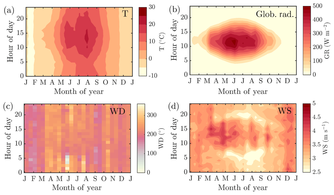
Figure 1 The seasonal evolution of diurnal cycles of ambient temperature measured at 4.2 m a.g.l. (a), global radiation above the forest canopy (b), wind direction above the forest canopy (c) and wind speed above the forest canopy (d) recorded at SMEAR II station in 2012–2018. The y axes in the figures represent the local time of day (UTC+2), and the x axes represent the time of the year. The color scales correspond to the temperature in degrees Celsius, global radiation in W m⁻², wind direction in degrees and wind speed in m s⁻¹, respectively. Panels (a), (b) and (d) include interpolation of the 14 d ×1 h resolution data grid into isolines based on the MATLAB 2017a contourf function. Panel (c) has no interpolation involved due to challenges related to interpolating over a circularly behaving variable. The plot is produced with MATLAB 2017a pcolor function.

2.2 ACSM measurements

The Aerosol Chemical Speciation Monitor (ACSM; Aerodyne Research Inc. USA) was first described by Ng et al. in 2011. It was developed based on the Aerosol Mass Spectrometer (AMS) (Canagaratna et al., 2007) but simplified at the cost of mass and time resolution to achieve a robust instrument for long-term measurements. The ACSM samples ambient air with a flow rate of 1.4 cm³ s⁻¹ through a critical orifice (100 µm in diameter) towards an aerodynamic lens, efficiently transmitting particles between approximately 75 and 650 nm in vacuum aerodynamic diameter (D_va) and passing through particles further up to 1 µm in D_va with a less efficient transmission (Liu et al., 2007). After this, the particles are flash vaporized at a 600 ^∘C hot surface in high vacuum and ionized with electrons from a tungsten filament (70 eV, electron impact ionization, EI). These processes lead to substantial fragmentation of the molecules forming the aerosol particles. The resulting ions are guided to a mass analyzer, a residual gas analyzer (RGA) quadrupole, scanning through different mass-to-charge ratios (m∕Q). The detector is a secondary electron multiplier (SEM). The particulate matter detected by the ACSM is referred to as non-refractory sub-micrometer particulate matter (PM₁). The word “non-refractory” (NR) is attributed to the instrument limitation to detect material flash evaporating at 600 ^∘C, thus being unable to measure heat-resistant material such as minerals or soot. The word “PM₁” is linked to the aerodynamic lens approximate cutoff at 1 µm. Importantly, the NR-PM₁ reported from these ACSM measurements is a difference between the signal of particle-laden air and signal recorded when the sampling flow passed a particle filter (filtered air).

The ACSM measurements for the current study were conducted within the forest canopy through the roof of an air-conditioned container. A PM_2.5 cyclone was used to filter out big particles that could cause clogging of the critical orifice. A Nafion dryer was installed in 2013 upstream of the instrument, ensuring a sampling relative humidity (RH) below 30 %. Before this, the RH was neither controlled nor recorded. Thus, the RH was likely high during summer but low during winter. Moreover, a 3 L min⁻¹ overflow, which was ejected only before the aerodynamic lens, was used to minimize losses in the sampling line (length approximately 3 m). The data were acquired using the ACSM data acquisition software (DAQ) provided by Aerodyne Research Inc., the instrument manufacturer. The DAQ version was updated upon new releases. The ACSM was operated to perform m∕Q scans with a 200 ms Th⁻¹ scan rate in the mass-to-charge range of m∕Q 10 Th to 140 Th. Filtered and particle-laden air were measured interchangeably for 28 quadrupole scans resulting in ca. 30 min averages. The air signal, obtained from the automatic filter measurements, was subtracted from the sample raw signal, yielding the signal from aerosol mass only. The data processing was performed using the ACSM local v. 1.6.0.3 toolkit within the Igor Pro v. 6.37 (Wavemetrics Inc., USA). Upon data processing, the different detected ions were assigned into organic or inorganic species bins (i.e., total organics, sulfate, nitrate, ammonium, and chloride) using a fragmentation table (Allan et al., 2004). Moreover, the data were normalized to account for N₂ signal variations related to ACSM flow rate and sensitivity changes (due to SEM voltage response decay).

The ACSM raw signal (IC) is converted to mass concentration (C) via the following equation obtained from Ng et al. (2011):

$$\begin{array}{}\text{(1)}& \begin{array}{rl}& C_s={\displaystyle \frac{\mathrm{1}}{\mathrm{CE}\times T_{\frac{m}{Q}}}}\times {\displaystyle \frac{{\mathrm{10}}^{\mathrm{12}}}{{\mathrm{RIE}}_s\times {\mathrm{RF}}_{{\mathrm{NO}}_{\mathrm{3}}}}}\\ & \times {\displaystyle \frac{Q_{\mathrm{cal}}\times G_{\mathrm{cal}}}{Q\times G}}\times \sum _{i=\mathrm{0}}^n{\mathrm{IC}}_{s,\mathrm{i}},\end{array}\end{array}$$

where C_s is the concentration of species s, CE is the particle collection efficiency (see Sect. 2.4), and T_m∕Q the m∕Q-dependent ion transmission efficiency in the RGA quadrupole mass analyzer. The T_m∕Q is constantly recorded based on naphthalene fragmentation patterns and their comparison to naphthalene fragmentation pattern in the NIST database (75 eV EI; http://webbook.nist.gov/, last access: 12 March 2020). Naphthalene is used as an internal standard in the ACSM and is thus always present in the mass spectrum (Ng et al., 2011). The RIE_s is the relative ionization efficiency of species s, and RF${}_{{\mathrm{NO}}_{\mathrm{3}}}$ is the ACSM response factor determined through ionization efficiency (IE) calibrations with ammonium nitrate (NH₄NO₃). The RF${}_{{\mathrm{NO}}_{\mathrm{3}}}$ explains the ACSM ion signal (A) per µg m⁻³ of nitrate. Q_cal and G_cal are the ACSM volumetric flow rate and detector gain during ACSM calibration, whereas Q and G are the values during the measurement period for volumetric flow rate and detector gain, respectively. They generally correspond to the calibration values. The final parameter is the sum of the signal introduced by individual ions (IC_s,i) originating from species s.

The ionization efficiency calibration was performed with dried and size-selected ammonium nitrate (NH₄NO₃) particles to retrieve the RF${}_{{\mathrm{NO}}_{\mathrm{3}}}$ parameter required in Eq. (1). In addition, ammonium sulfate ((NH₄)₂SO₄) calibrations were carried out, albeit less frequently, providing a value for the sulfate relative ionization efficiency (RIE${}_{{\mathrm{SO}}_{\mathrm{4}}}$). RIE${}_{{\mathrm{NH}}_{\mathrm{4}}}$ was derived from the ammonium nitrate calibration. Constant RF and RIE values were used for each year, respectively. The conversion from ACSM raw signal to mass concentration was performed with the ACSM Local v. 1.6.0.3 provided by Aerodyne Research Inc.

2.3 Additional measurements

In addition to the ACSM measurements, the SMEAR II station has a large number of other air-composition-related measurements. In the current study, we investigate only a small fraction of them. The particle measurements, i.e., ACSM, Differential Mobility Particle Sizer (DMPS), Dekati cascade impactor, aethalometer, Organic Carbon and Elemental Carbon (OCEC) analyzer, and Monitor for AeRosols and Gases in ambient Air (MARGA) 2S, were conducted in two measurement containers and a cabin, all located within ca. 50 m from each other. The gas-phase sampling of NO_x, SO₂, CO, and VOCs as well as temperature, wind, and global radiation measurements, were conducted from a station mast that has several measurement heights from near the ground up to 127 m height. The temperature measurement was conducted with a Pt100 sensor (4.2 m a.g.l.), and the global shortwave radiation measurement was performed with a Middleton SK08 pyranometer (125 m a.g.l.). The horizontal wind measurements were conducted with Thies 2D Ultrasonic anemometers above the forest canopy (16.8 to 67.2 m a.g.l.). The NO_x measurements were performed with a TEI 42 iTL chemiluminescence analyzer equipped with a photolytic Blue Light Converter (NO₂ to NO), SO₂ was measured with a TEI 43 iTLE fluorescence analyzer, and CO was measured with IR absorption analyzers Horiba APMA 370 (until January 2016) and API 300EU (from February 2016 onwards). The NO_x, SO₂, CO, and proton transfer reaction quadrupole mass spectrometer (PTR-MS) sampling was conducted 67.2 m a.g.l. The SO₂, NO_x, CO, PTR-MS (only 2012–2013), and meteorology data were uploaded from SmartSMEAR database (https://avaa.tdata.fi/web/smart, last access: 11 March 2020) (Junninen et al., 2009). The DMPS, Dekati impactor, aethalometer, OCEC analyzer, and MARGA-2S measurements conducted within the forest canopy are described in more detail in the sections below. The data availability is shown in Fig. A2.

2.3.1 DMPS

The Differential Mobility Particle Sizer (DMPS) measures the aerosol size distribution below 1 µm electrical mobility diameter. SMEAR II holds the world record in online aerosol size distribution measurements (Dada et al., 2017), as the measurements had already started in 1996. The DMPS system is described in detail previously (Aalto et al., 2001). Briefly, the SMEAR II DMPS is a twin DMPS setup that samples 8 m a.g.l. from an inlet with a flow rate of 150 L min⁻¹. The measurement cycle is 10 min. The first DMPS (DMPS-1) has a 10.9 cm long Vienna-type differential mobility analyzer (DMA) and a model TSI3025 condensation particle counter (CPC) that was changed to model TSI3776 after October 2016. The sheath flow rate in the DMA is 20 L min⁻¹, and the aerosol flow rate is 4.0 L min⁻¹. The measurement range of the DMPS-1 is 3–40 nm. The second DMPS (DMPS-2) has a 28 cm long Vienna type DMA and a TSI3772 CPC. The sheath flow rate is 5 L min⁻¹ and the aerosol flow rate 1 L min⁻¹. The measurement range is 20 nm–1 µm. The sheath flows are dried (RH <40 %), controlled with regulating valves, and measured with TSI mass flow meters operated in volumetric flow mode. The aerosol flow is brought to charge balance with 370 MBq C-14 and, after March 2018, with a 370 MBq Ni-63 radioactive beta source. The aerosol flow rates are monitored with pressure drop flow meters. The aerosol flows were not dried. Temperatures and RHs are monitored from DMPS excess flow and from the aerosol inlet. The aerosol flow rates were checked and adjusted every week against a Gilian Gilibrator flow meter throughout the measurement period. The DMA high voltages were also validated with a multimeter. The CPC concentrations were compared against each other with size-selected ammonium sulfate particles in the 6–40 nm range and also compared against the TSI3775 particle counter that measures the total aerosol particle number concentration at the station. The sizing accuracy of the two DMAs were cross-compared with 20 nm ammonium sulfate particles. In addition, the accuracies of the RH, temperature, and pressure probes were validated each year.

2.3.2 Cascade impactor

The PM₁ and PM_2.5 (particulate mass of aerosol particles with an aerodynamic diameter below 2.5 µm) mass concentrations measured between 2012 and 2017, which were included in the current study, were retrieved from the cascade impactor measurements. This gravimetric PM₁₀ impactor, produced by Dekati Ltd., is a three-stage impactor with cut points at 10, 2.5 and 1 µm. The collection is conducted on greased (Apiezon vacuum grease diluted in toluene) Nuclepore 800 203 25 mm polycarbonate membranes with 30 L min⁻¹ flow rate, approximately 5 m a.g.l. The filter smearing was performed to avoid losses due to particle bouncing. The filters were weighed manually every 2–3 d and stored in a freezer for possible further analysis.

2.3.3 PTR-MS

The monoterpene concentration was measured using the proton transfer reaction quadrupole mass spectrometer (PTR-MS) manufactured by Ionicon Analytik GmbH, Innsbruck, Austria (Lindinger and Jordan, 1998). The monoterpene measurement setup has been described in detail previously (Rantala et al., 2015). In short, the PTR-MS was placed inside a measurement cabin on the ground level, and the sample air was drawn down from a measurement mast to the instrument using 157 m long PTFE tubing (16 mm o.d. and 14 mm i.d.). The sampling line was heated and the sample flow was 45 L min⁻¹. However, the sample entering the PTR-MS was only 0.1 L min⁻¹. During the study period, the primary ion signal H₃O⁺ (measured at isotope m∕Q 21 Th) varied slightly around 5–30×10⁶ c.p.s. (counts per second). The instrument was calibrated every 2–4 weeks using three different VOC standards (Apel–Riemer), and the instrumental background was measured every third hour using VOC-free air produced by a zero air generator (Parker ChromGas, model 3501). Normalized sensitivities and the volume mixing ratios were then calculated using the method introduced previously (Taipale et al., 2008). For example, the normalized sensitivity of α-pinene (measured at m∕Q 137 Th) varied between 2 and 5 n.c.p.s. ppb⁻¹ over the study period. Only the signal of monoterpenes at m∕Q 137 Th were analyzed in the current study.

2.3.4 Aethalometer

The concentration of equivalent black carbon (eBC) in the PM₁ size range was measured by using two different Magee Scientific aethalometer models: AE-31 during 2012–2017 and AE-33 in 2018. The sample air was taken through an inlet, equipped with a PM₁₀ cyclone and a Nafion dryer, and a PM₁ impactor. Aethalometers determine the concentration of eBC by collecting aerosols on a filter medium and measuring the change in light attenuation through the filter. Both of the aethalometers quantify eBC concentration optically at seven wavelengths (370, 470, 520, 590, 660, 880, and 950 nm). Only the eBC concentration determined at 880 nm was used in the current study. AE-31 data were corrected for a filter loading error with a correction algorithm derived previously (Collaud Coen et al., 2013). A mass absorption cross section of 4.78 m² g⁻¹ at 880 nm was used in the eBC concentration calculation. The AE-33 used a “dual-spot” correction, which has been described previously (Drinovec et al., 2015).

2.3.5 OCEC analyzer

Organic carbon (OC) and elemental carbon (EC) concentrations were measured using a semicontinuous Sunset OCEC analyzer (Bauer et al., 2009) produced by Sunset Laboratories Inc. (USA). The aerosol sampling was conducted through the same container roof as the ACSM. The inlet length was approximately the same as for the ACSM (ca. 3 m). The sample flow was guided through a PM_2.5 cyclone and a carbon plate denuder to avoid collection of large particles and a positive artifact introduced by organic vapors. In the OCEC, the sample is collected on a quartz filter for 2.5 h with an 8 L min⁻¹ flow rate. The sampling procedure is followed by the analysis phase. The analysis phase includes thermal desorption of PM from the filter following the EUSAAR-2 protocol (Cavalli et al., 2010), and introducing the aerosol sample to inert helium gas that is used to carry the OC to a MnO₂ oxidizing oven. This leads to OC oxidation to CO₂, which is then quantified with a nondispersive infrared (NDIR) detector. Afterwards the remaining sample is introduced to a mixture of oxygen and helium, enabling EC transfer to the oven. The resulting CO₂ from EC desorption and combustion is also quantified using the NDIR detector. An additional optical correction was used to account for the amount of pyrolyzed OC during the helium phase. EC was also quantified using a laser installed in the analyzer. This method is similar to the aethalometer (see Sect. 2.3.4). After each analysis phase, a calibration cycle was performed via methane oxidation. The instrument was maintained extensively in November 2017, thus making the year 2018 most reliable for ACSM comparison. Only data measured in 2018 was used in this study.

2.3.6 MARGA-2S

Inorganic gases (HCl, HNO₃, HONO, NH₃, SO₂) and major inorganic ions in PM_2.5 and PM₁₀ fraction (Cl⁻, ${\mathrm{NO}}_{\mathrm{3}}^{-}$, ${\mathrm{SO}}_{\mathrm{4}}^{\mathrm{2}-}$, ${\mathrm{NH}}_{\mathrm{4}}^{+}$, Na⁺, K⁺, Mg²⁺, Ca²⁺) were measured with 1 h time resolution using the online ion chromatograph MARGA 2S ADI 2080 (Applikon Analytical BV, the Netherlands). In the MARGA instrument, ambient air was taken through the inlet to a wet rotating denuder where the gases were diffused in absorption solution (10 ppm hydrogen peroxide). Aerosol particles that passed through denuder were collected in a steam jet aerosol collector. The sample solutions from the denuder and the steam jet aerosol collector were collected in syringes and injected in an anion and cation ion chromatograph with an internal standard solution (LiBr). Cations were separated in a Metrosep C4 (100∕4.0) cation column using 3.2 mmol L⁻¹ MSA eluent. For anion separation, we used a Metrosep A Supp 10 (75∕4.0) column with an eluent comprised of Na₂CO₃ and NaHCO₃ (7 mmol L⁻¹∕8 mmol L⁻¹). The detection limits for all the components were 0.1 µg m⁻³ or smaller. The unit used for the current study has been described in more detail previously (Makkonen et al., 2012).

2.4 ACSM collection efficiency correction

The ACSM data processing includes correcting for the measurement collection efficiency (CE) that is estimated to be approximately 0.45–0.5 on average for AMS-type instruments (Middlebrook et al., 2012). The reduction is caused by particle bouncing at the instrument vaporizer (Middlebrook et al., 2012). Middlebrook et al. (2012) provide a method to estimate the CE based on aerosol chemical composition. However, this method was not applicable to our data set due to low, and thus noisy, ammonium signals that were most of the time near the instrument detection limit. Thus, we chose to calculate the collection efficiency based on the ratio between the NR-PM₁ (total mass concentration measured by the ACSM) and a Differential Mobility Particle Sizer (DMPS)-derived mass concentration (after subtracting the equivalent black carbon, eBC). The DMPS-derived mass concentration is determined as follows: (1) calculation of aerosol volume concentration (m³ m⁻³) of the ACSM detectable size range, where the aerodynamics lens transmission is most efficient (50–450 nm in electrical mobility = ∼75–650 nm in vacuum aerodynamic diameter) and assuming spherical particles; (2) estimating aerosol density based on the ACSM-measured chemical composition (${\mathit{\rho }}_{({\mathrm{NH}}_{\mathrm{4}}{)}_{\mathrm{2}}{\mathrm{SO}}_{\mathrm{4}}}=\mathrm{1.77}$ g cm⁻³, ${\mathit{\rho }}_{{\mathrm{NH}}_{\mathrm{4}}{\mathrm{NO}}_{\mathrm{3}}}=\mathrm{1.72}$ g cm⁻³, ρ_Org=1.50 g cm⁻³, ρ_BC=1.00 g cm⁻³); and (3) calculating the mass concentration (µg m⁻³; mass concentration = density × volume concentration). As direct scaling of ACSM data to the DMPS-derived and eBC subtracted mass concentration is strongly not recommended, we chose to use 2-month running medians of the ratio between the NR-PM₁ and eBC-subtracted DMPS-derived mass concentration. The 2-month running median approach diminishes the effect of instrument noise in the DMPS-derived mass concentration that could otherwise be introduced as additional uncertainty into the ACSM data. The 2-month median CEs were within 10 % of the annual mean values in the years 2013–2018. In 2012 the CE had stronger seasonal variation (16 % variation around the mean, peaking in summer), likely due to the lack of the aerosol dryer in the sampling line. The magnitudes of the CEs can be obtained from Fig. 2a.

Figure 2 (a) The NR-PM₁ mass concentration without collection efficiency (CE) correction vs. the DMPS-derived eBC subtracted mass concentration. The linear fits are displayed with solid lines for each year. The slopes of the linear fits (k) and Pearson correlation coefficients (R²) are presented in the figure legend. (b) CE-corrected NR-PM₁ mass concentration vs. the DMPS-derived eBC subtracted mass concentration. The black line represents the overall linear fit. (c) The NR-PM₁ mass concentration without collection efficiency (CE) correction vs. the Dekati impactor PM₁ concentration. The linear fits are displayed with solid lines for each year, respectively. (d) CE-corrected NR-PM₁ mass concentration vs. correction vs. the Dekati impactor PM₁ concentration. The linear fits are displayed with solid lines for each year. (e) The ACSM organics vs. the PM_2.5 organic carbon (OC) detected with a semicontinuous OC/EC analyzer. The dashed black line represents the overall linear fit (Pearson R²=0.72), and the solid orange and pink linear fit lines represent the February and July fits, respectively. The color coding indicates the month of the year in 2018. (f) The ACSM sulfate vs. the PM_2.5 sulfate detected with MARGA-2S. The black line represents the overall linear fit. In all of the panels, dots represent all the measurement points collected in the course of the measurement period.

Figure 2a depicts the linear regression fits for ACSM mass concentration (without CE correction) and eBC-subtracted DMPS-derived mass concentration scatter plots for each year. The correlation coefficients (Pearson R²) between these two independently measured variables are high, indicating that both ACSM and DMPS functioned well throughout the long data set. The years 2012 and 2016–2018 have linear regression fit slopes (k) corresponding to CE values reported in the literature (Middlebrook et al., 2012), whereas slopes for the years 2013–2015 were higher than expected. The most likely reason for these high values were calibration difficulties that might have led to underestimation of the instrument RF${}_{{\mathrm{NO}}_{\mathrm{3}}}$ that is required in the mass concentration calculation. This possible RF${}_{{\mathrm{NO}}_{\mathrm{3}}}$ underestimation was accounted for in the DMPS-based CE correction with higher CE values than theoretically suggested for ACSM systems. The resulting agreement between the eBC-subtracted DMPS-derived mass concentration and the CE-corrected ACSM-derived mass concentration is presented in Fig. 2b. As the NR-PM₁ incorporates the 2-month running median of the CE calculated using DMPS data, it is not surprising that a good correlation was achieved.

Figure 2c and d visualize the relationship between ACSM-derived mass concentration and a Dekati impactor PM₁ data (see Sect. 2.3.2) before and after CE correction, respectively. The impactor PM₁ is not eBC subtracted as it would have significantly decreased the number of points in the analysis. The degree of agreement between the ACSM and impactor measurements is significantly lower compared to the agreement between the ACSM and DMPS. The reason for this is likely the fact that the Dekati impactor measurements are prone to uncertainties due to long sampling times and manual weighing. This scatter is reduced slightly in Fig. 2d compared to Fig. 2c due to the DMPS-based CE correction and the slope value (k) increase. As the agreement between the ACSM-derived mass concentration and impactor PM₁ is better after CE correction, due to both increased correlation coefficients (R²) and slopes (k), the (2-month running median) DMPS-based CE correction is justified. Hereafter, all the ACSM data presented and discussed are CE corrected. We refer to it as NR-PM₁. The CE correction method applied importantly also ensures more quantitative year-to-year comparability of the ACSM data acquired, as it also corrected for the overestimated calibration values obtained during 2013–2015.

2.5 ACSM chemical speciation validation

To validate the ACSM chemical speciation process, the ACSM organics (Org) and sulfate (SO₄) were compared against the organic carbon (OC) was measured by a Sunset OCEC analyzer (see Sect. 2.3.5) (Fig. 2e) and water-soluble sulfate measured by a MARGA-2S (see Sect. 2.3.5) (Fig. 2f), respectively. Both of these reference instruments sample the PM_2.5 range, and thus we expect them to also detect larger particles and thus a higher mass loading than the ACSM, when particles exceeding 1 µm in aerodynamic diameter are present in the ambient air. The OC and Org measurements show a high degree of agreement, indicated by Pearson R² of 0.72 during the overlapping measurement period at SMEAR II. The slope of the linear regression fit (k=1.52) is comparable to literature values of organic matter to organic carbon ratios (OM:OC) (Turpin and Lim, 2001; Lim and Turpin, 2002; Russell, 2003). The linear regression is calculated using all the overlapping data from the year 2018, when the OCEC was functioning well after instrument service. Regarding the water-soluble inorganic ions, only the ${\mathrm{SO}}_{\mathrm{4}}^{\mathrm{2}-}$ concentration (in PM_2.5), retrieved from the MARGA measurements, was used for the current analysis for ACSM data validation purposes. The nitrate time series, for example, are known to be different between the two measurements at SMEAR II (Makkonen et al., 2014). The scatter between the nitrate measurements, also visualized here, in Fig. A3, could serve as evidence of organic nitrates, which are not efficiently detected by MARGA (Makkonen et al., 2014). The presence of organic nitrates are discussed later in the paper (see Sect. 3.2). Other factors influencing the nitrate agreement could arise from the MARGA nitrate background subtraction procedure, the overall low nitrate signal at SMEAR II (Makkonen et al., 2014), an organic CH₂O⁺ fragment coinciding with NO⁺ at m∕Q 30 Th, leading to ACSM nitrate overprediction under certain conditions, and the difference between the ACSM and MARGA size cuts (PM₁ vs. PM_2.5). The ACSM sulfate, however, correlates well with MARGA (Pearson R²=0.77) but has a slightly lower Pearson R² compared to an earlier <11-month MARGA vs. AMS comparison from SMEAR II (Pearson R²=0.91) (Makkonen et al., 2014). Overall, based on the good agreement between ACSM and Sunset OCEC, MARGA, DMPS, and Dekati cascade impactor measurements, we are confident of the year-to-year comparability of our ACSM data set.

2.6 Openair polar plots with ZeFir pollution tracker

The wind direction dependence of different NR-PM₁ chemical species observed at SMEAR II were investigated with openair bivariate polar plots. Openair is an open-source, R-based package described previously (Carslaw and Ropkins, 2012). Briefly, the openair polar plots show how the pollutant concentration varies under different wind speed and direction. The calculation of the polar plots are based on binning pollutant concentration data into different wind direction and speed bins, followed by the concentration field interpolation. As the polar plots do not take the frequencies of the wind direction nor wind speed into account, they should be investigated together with a traditional wind rose, representing the likelihood of each wind direction and wind speed combination. The ZeFir pollution tracker (Petit et al., 2017), an Igor Pro (Wavemetrics Inc, USA) graphical interface for producing openair polar plots, among other functionalities, was utilized in the current study. Median statistics with fine resolution were set in the ZeFir-based openair initialization. These plots provide an informative first step for tracking PM₁ and its precursors' wind direction and speed dependence.

3 Results and discussion

First, we state that the ACSM data set was not long enough to provide sufficient statistics for investigation of long-term trends of NR-PM₁ or its components' loading, hence no analysis of such is presented here. In this section we discuss the inter- and intra-annual variation in sub-micrometer non-refractory aerosol chemical composition at SMEAR II in 2012–2018. We first introduce the monthly scale behavior and year-to-year variability. We briefly introduce two case studies, one linked to elevated sulfate loading at the station due to a lava field eruption in Iceland and another discussing the effect of heat waves on PM₁ loading and composition. Hereafter, we introduce the overall median diurnal profiles of individual chemical species observed in the NR-PM₁ and the chemical composition observations linked to wind speed and direction observations above the forest canopy.

3.1 Inter- and intra-annual variation

The monthly median seasonal cycles of NR-PM₁ and PM_2.5 show bimodal distributions, as the PM loading has two maxima: one peak in February and another in summer (June, July, and August); the latter being more significant. This can be observed from Fig. 3a and b, where the monthly median PM loading for each year is visualized. The NR-PM₁ seasonal cycle (Fig. 3a) is more pronounced compared to the PM_2.5 cycle (Fig. 3b). A possible reason for this could be the lack of PM_2.5 data in 2018 that has a high impact on the NR-PM₁ July peak. The PM₁ ∕ PM_2.5 ratio (Fig. 3c) in turn, calculated using the Dekati Impactor data alone, demonstrates that most of the time 60 %–80 % of PM_2.5 can be explained by PM₁. The ratio is lowest (60 %–70 %) in wintertime (December, January, February), implying an increased mass fraction of particles with aerodynamic diameters greater than a micrometer compared to the summertime when the ratio is nearly 80 %.

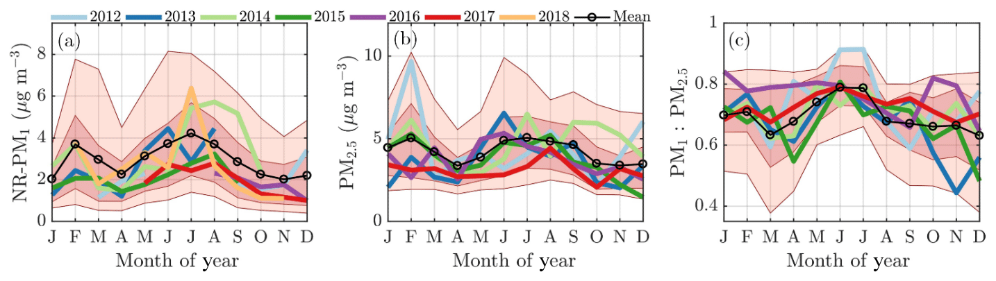
Figure 3 The monthly cycles of NR-PM₁ (a), PM_2.5 (b), and the ratio between PM₁ and PM_2.5 (c). The median monthly values for each year are individually displayed with the colored solid lines. The circled black line represents the overall monthly mean values. The shaded dark red area is drawn between the overall 25th and 75th percentiles and the shaded lighter red area is drawn between the overall 10th and 90th percentile. The x axes represent the time of the year and the y axes in panels (a) and (b) represent mass concentration in µg m⁻³ and a unitless ratio in (c).

The February PM maximum is linked to an enhanced loading of inorganic aerosol species, such as nitrate and especially sulfate, as well as a slight increase in organics (Fig. 4a–c), whereas the summertime maximum is explained by a massive enhancement of organics alone (Fig. 4a). The main precursors for inorganic aerosols, i.e., SO₂ and NO_x, peak during winter albeit less sharply than in February alone (Fig. 4e and f). As fossil fuel combustion processes are the major sources of SO₂ and NO_x, their emissions likely increase during cold months due to enhanced need for residential heating, for example. More importantly, these emissions are trapped in a shallow atmospheric boundary layer, increasing the concentration recorded within it. One possible reason for the “lack” of sulfate and nitrate aerosol outside February, despite the great availability of SO₂ and NO_x, is likely related to wind direction transitioning, discussed later in the paper. Another effect could be the darkness prohibiting photochemistry needed for inorganic aerosol formation. Indeed, the global radiation measured above the forest canopy shows only a minimal shortwave radiation flux in November, December, and early January, but it increases from mid-January onwards (Fig. 1b). As February is generally drier (in terms of less precipitation) than the other winter months (Pirinen et al., 2012), the lifetime of aerosols could be greater, making the inorganic particles more likely to reach SMEAR II. The inorganic nitrate (ammonium nitrate) formation is highly dependent on ammonia availability. The ammonia concentration during wintertime is nearly negligible at SMEAR II and increases rapidly in spring (Makkonen et al., 2014). The low nearby ammonia availability suggests that the wintertime nitrate is long-range transport.

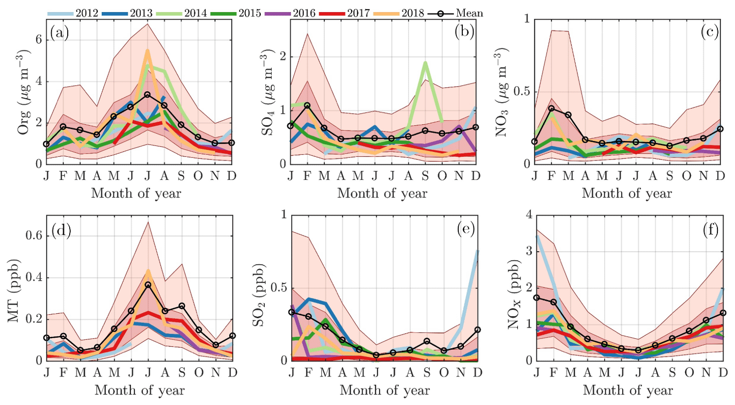
Figure 4 The monthly cycles of organics (a), sulfate (b), and nitrate (c) concentrations in the NR-PM₁ and their major precursors, i.e., monoterpenes (d), sulfur dioxide (e), and nitrogen oxides (f). The median monthly concentrations for each year are individually displayed with the solid colored lines. The circled black line represents the overall monthly mean values. The shaded dark red area is drawn between the overall 25th and 75th percentiles, and the shaded lighter red area is drawn between the overall 10th and 90th percentile. The x axes represent the time of the year and the y axes in panels (a)–(c) represent mass concentration in µg m⁻³ and (d)–(f) in parts per billion (ppb).

Monoterpenes also show a nonzero loading during all winter months (Fig. 4d). Their source is likely anthropogenic, such as the nearby sawmills, rather than biogenic due to the low ambient temperature limiting their biogenic emissions (Guenther et al., 1993; Hakola et al., 2012; Kontkanen et al., 2016). Their wintertime presence could be linked to their overall decreased photochemical sink and them being emitted to the shallower atmospheric boundary layer with little vertical dilution. The monoterpene mixing ratio starts increasing rapidly in April, achieving its maximum monthly median value during July (Fig. 4d), simultaneous with NR-PM₁ organics (Fig. 4a). Previous studies have shown that monoterpene emissions increase exponentially with ambient temperature (Guenther et al., 1993; Aalto et al., 2015). As the current study does not incorporate monoterpene emission data, we visualize the behavior of monoterpene mixing ratio with increasing ambient temperature in Fig. 5b. The increase in monoterpene mixing ratio is likely a combined result from increased biological plant activity in the forest and the increased emissions due to higher temperature. Organic aerosol concentration behaves in a similar manner as a function of temperature, as depicted in Fig. 5a. Such behavior in organic aerosol loading is often attributed to biogenic SOA formation from BVOCs (Daellenbach et al., 2017; Stefenelli et al., 2019; Vlachou et al., 2018; Paasonen et al., 2013).

Besides biogenic SOA, open fire biomass burning organic aerosol (BBOA) is also a major contributor to summertime organics worldwide, from wildfires during dry conditions (Bond et al., 2004; De Gouw and Jimenez, 2009; Mikhailov et al., 2017; Corrigan et al., 2013). An enhancement in eBC concentration, a tracer for BBOA, was observed as a function of temperature at SMEAR II, implying the possible presence of BBOA in the summertime sub-micrometer aerosol (Fig. 5d). However, uncertainties can be attributed to the eBC concentration as scattering coatings, such as salts or even photochemically aged SOA, can also generate a lensing effect, leading to an overestimation of eBC (Bond and Bergstrom, 2006; Zhang et al., 2018). Such an effect could lead to a substantial overestimation of eBC, especially in summertime when the organic loading is highest. Some certainty of the BBOA and BC enhancement with high temperatures can, however, be retrieved from Fig. 5c, where carbon monoxide (CO) mixing ratio also increases at relatively high ambient temperatures (T>15 ^∘C). CO is known to be emitted from incomplete combustion processes. Nonetheless, as the increase in eBC visualized in Fig. 5d is less drastic than for monoterpenes, we suggest the biogenic SOA production as the major organic aerosol source in summertime. While the quantification and separation of BBOA from SOA will be the topic of an upcoming independent publication centered on the analysis of organic aerosol mass spectral fingerprints at SMEAR II, we briefly introduce the behavior of f₆₀. f₆₀, which equals the contribution of m∕Q 60 Th signal to the total organic signal recorded by the ACSM, is a marker for levoglucosan-like species originating from cellulose pyrolysis in biomass burning (Schneider et al., 2006; Alfarra et al., 2007). f₆₀ is present at high percentages in fresh BBOA plumes (Cubison et al., 2011) but decays due to BBOA photochemical aging into oxidized organic aerosol. The fairly rapid (on the order of several hours to days) photochemical aging of BBOA has been a topic of earlier chamber (Grieshop et al., 2009; Jimenez et al., 2009) and ambient studies (DeCarlo et al., 2010; Cubison et al., 2011). Here, unlike CO and eBC, f₆₀ does not increase as a function of temperature in the highest temperature bins but stays rather constant, albeit lower than the f₆₀ values recorded under cold temperatures at SMEAR II (Fig. 5e). As the possible wildfires contributing to SMEAR II CO and eBC under high ambient temperatures also occur further away, it is likely that the BBOA is oxidized before it is detected at SMEAR II. CO and eBC can be considered as more inert BBOA markers compared to f₆₀. The wintertime f₆₀ is likely linked to wintertime biomass burning (for domestic heating purposes) emissions trapped in the shallow mixing layer. These emissions are discussed more later on in the paper (see Sect. 3.2).

3.1.1 Case study: the effect of warm summers on organic aerosol loading

The highest NR-PM₁ mass concentrations were detected during the summers of 2014 and 2018. These summers were the hottest during the whole measurement period (Fig. 6a), and linked to persistent high pressure conditions (Sinclair et al., 2019; FMI, 2014). The nonparametric probability densities (kernel distributions) for temperature for July in 2012–2018, displayed individually in Fig. 4a, clearly show higher temperatures in July 2014 and 2018. Indeed, these months were abnormally warm as July 2014 and July 2018 were 2.2 ^∘C and 3.4 ^∘C higher than the 7-year July mean (16.6 ^∘C), respectively. Compared to the 30-year July climate at SMEAR II (1981–2010) (Pirinen et al., 2012), the mean temperature in July 2014 and July 2018 were 2.8 ^∘C and 4.0 ^∘C higher, respectively. As can be seen from Fig. 4a and d, both organic aerosol and monoterpene concentration positively responded to this temperature change with high median values. The same phenomenon is visualized in Fig. 4b and c through kernel densities for particulate organics and monoterpenes, respectively, for July of each year. The recorded organic aerosol concentration was 50 % higher and 70 % higher than the 7-year mean in July 2014 and 2018, respectively. The monoterpene concentration in turn was 50 % higher in 2018 compared to the mean of all available July data (due to PTR-MS sensitivity issues, the 2014 data were chosen to be excluded from the analysis).

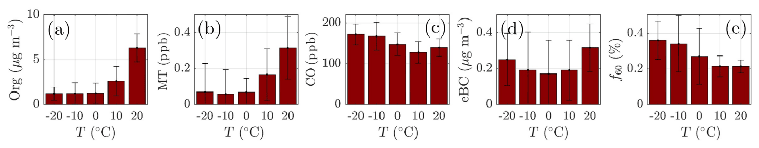
Figure 5 The daily mean organic aerosol (Org, a), monoterpene (MT, b), carbon monoxide (CO, c), equivalent black carbon (eBC, d) concentrations, and the fraction of the ACSM Org signal made up by levoglucosan-like species (f₆₀, e) recorded under different ambient temperatures. The values recorded are assigned into 10 ^∘C wide bins based on the daily ambient temperature mean. The marker error bars show the standard deviation of the values in each bin.

As the high-pressure weather ruling in July 2014 and 2018 further promoted clear-sky conditions, the oxidation capacity of the air was also likely affected. This could have led to efficient monoterpene oxidation towards condensable low-volatility products. Furthermore, their condensation onto particles could explain the observed high organic aerosol mass concentration. The SOA formation enhancement as a function of temperature has also been investigated previously in a modeling study, where a significant global increase in monoterpene-derived organic aerosol concentration was projected to future, following different climate scenarios introduced by the Intergovernmental Panel of Climate Change (IPCC) (Heald et al., 2008). Kourtchev et al. (2016) investigated the effect of high ambient temperature on biogenic SOA loading and composition utilizing measurement data from SMEAR II. They include the summers of 2011 and 2014 in their analysis, where summer 2011 represents a significantly colder summer (average ambient temperature was 8 ^∘C less than in 2014). By utilizing ultra-high-resolution offline mass spectrometry on filter samples collected at SMEAR II, they detected a significantly higher SOA oligomer content during 2014. Their results not only highlight the large increase in SOA mass as a function of temperature but also the SOA composition differences affected by the large SOA content that further influenced the CCN formation potential of SOA.

A quick revisit of the OCEC vs. ACSM comparison performed earlier in the paper (Fig. 2e) shows relatively high Org ∕ OC values (k=1.68) for July 2018, which further indicates high oxygenation of OA (Aiken et al., 2008). However, the time series of the ruling monthly Org ∕ OC values, visualized in Fig. A5, reveal an even higher Org ∕ OC for August 2018. Further analysis of Org ∕ OC recorded from SMEAR II is needed to answer whether such behavior is frequently occurring at SMEAR II, or whether July 2018 organic aerosol was less functionalized (oxidized) than usual due to higher presence of primary organic aerosol, such as BBOA, than usual. Thus, in order to not link the organic aerosol increase to biogenic SOA formation exclusively, we also investigated the presence of BBOA in the sub-micrometer aerosol during July 2014 and 2018 via kernel distributions for eBC and f₆₀, as presented in Fig. 6d and e. The eBC distribution clearly hints towards BBOA presence during July 2018, whereas July 2014 seems much less affected. Importantly, we also want to inform that in July 2018 we had only 1 week of eBC data available. The July 2018 eBC could be linked to the severe wildfires occurring in Sweden during July and August 2018. The July eBC measurement period overlaps with the forest fire occurrence period. Sweden also suffered from wildfires in August 2014, which are not depicted in Fig. 6 because it focuses on months of July alone. The f₆₀ in turn follows the conclusions made earlier in the context of Fig. 5 as the f₆₀ values remain low each July, and approach thef₆₀ background levels of 0.3 % (Cubison et al., 2011; Fig. 6e). Importantly, such negligible f₆₀ signals were detected under the influence of an aged BBOA plume originating from Moscow and northern Ukraine wildfires at SMEAR II in 2010 as well (Corrigan et al., 2013). An AMS, which was used as one of the measurement tools in the campaign, detected mass spectra resembling oxidized organic aerosol during the biomass burning influence. These data correlated well with multiple biomass burning markers including CO, potassium, and acetonitrile despite the lack of resemblance with fresh BBOA mass spectra with high f₆₀. Corrigan et al. (2013) finally attributed up to 25 % of the organic aerosol to BBOA originating from the Moscow and northern Ukraine wildfires. A total of 35 % of the organic aerosol mass was associated with biogenic SOA formation. The weather during the Corrigan et al. (2013) study period in 2010 was also unusually warm (T_avg=20 ^∘C) and resembled summers 2014 and 2018 regarding the ruling anticyclonic circulation pattern.

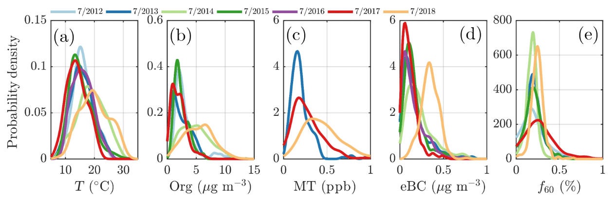
Figure 6 Nonparametric probability densities (kernel distributions) of temperature (a), organic aerosol (b), monoterpenes (c), equivalent black carbon (d) concentrations, and the fraction of the ACSM organic signal made up by levoglucosan-like species (f₆₀; e) during individual months of July across the measurement period (2012–2018). The data availability for eBC was 1 week in July 2018. The x axes represent the T, Org, MT, and eBC values recorded, respectively, and the y axes the nonparametric probability densities. Briefly, the kernel distributions are similar to smoothed histograms of the measurement data. This visualization was chosen to avoid assumptions of the nature of distribution that might hide important features of the measurement data if presented with normal distributions, for instance.

The frequency, duration, and intensity of heat waves are projected to increase in the future Finnish climate due to positive pressure anomalies over Finland and to the east of Finland, as well as a negative pressure anomaly over Russia between 90 and 120^∘ E (Kim et al., 2018). Moreover, the IPCC states that droughts and insect outbreaks are projected to be boosted in the warming climate (IPCC, 2014). Recent findings by Zhao et al. (2017) show how such biotic and abiotic stress factors enhance VOC emissions from plants that further contribute to organic aerosol after oxidation (Zhao et al., 2017). Wildfires in turn are likewise globally likely to occur more frequently in the future due to the increasing number of long-lasting heat waves (Spracklen et al., 2009). Indeed, BBOA loadings due to wildfires already show a slight increase in the United States (Ridley et al., 2018). Based on these previous studies, as well as our observations together with the Corrigan et al. (2013) study from SMEAR II, the increasing frequency of heat waves and wildfires will enhance the particulate matter loading at SMEAR II in the future, and continuous long-term measurements, like the ones presented here, will be important in monitoring such changes.

3.1.2 Case study: sulfate transport from Holuhraun flood lava eruption

The sulfate loading in September 2014 represents the largest outlier in Fig. 4b, with the average mass concentration 5 times greater than the overall September mean. The mean SO₂ concentration during September 2014 was 0.66 ppb, which is 0.50 ppb higher than the mean SO₂ mixing ratio representing all the Septembers during the measurement period (0.16 ppb). The elevated median SO₂ concentration during September 2014 is also visible in Fig. 4e. To investigate the source of sulfur, we displayed the full atmospheric column SO₂ concentration during September 2014 utilizing satellite observations (Fig. A6a). The SO₂ concentration hot spot was located in Iceland and is linked to the fissure Bárðarbunga–Veiðivötn eruption at Holuhraun (31 August 2014–28 February 2015) that yielded 20–120 kt d⁻¹ of SO₂ (Schmidt et al., 2015). The concentration above SMEAR II was obviously not comparable to the loading near the eruption site. However, based on a rough trajectory analysis (Fig. A6b), we link our observations of elevated sulfate and SO₂ during September 2014 to the diluted plume from Holuhraun.

3.2 Diurnal variation in NR-PM₁ composition

The year-to-year variation in the NR-PM₁ monthly median seasonal cycles shows rather consistent behavior throughout the measurement period, and even the overall 10th percentile of the PM data suits the bimodal trend discussed in the section above. The 10th percentile also agrees with the seasonal trends associated with individual NR-PM₁ chemical species, i.e., organics, sulfate, and nitrate, as well as their precursors (Fig. 4). A few observed outliers are discussed in the sections above (see Sect. 3.1.1 and 3.1.2). As the year-to-year variability is rather minimal, we decided to investigate the overall median temporal behavior of aerosol chemical composition further via Fig. 7. The subplots in this figure are based on data matrices of median diurnal cycles (1 h resolution) for every 2 weeks of a year (24×26 matrix). The matrices are visualized with contour plots (contourf, MATLAB 2017a) except for Fig. 7h, due to the high noise level of the time trace.

Figure 7 The median diurnal cycles of NR-PM₁ (a), organic to inorganic ratio (b), organic aerosol (c), sulfate (d), nitrate (e), ammonium (f), m∕Q  30 : m∕Q46 Th fragmentation ratio (g), and the ratio between measured and predicted ammonium (h). The y axes represent the local time of day (UTC+2), and the x axes represent the month. The color scales present the mass concentration (a, c–f) or ratios (b, g–h). Note that the scaling of the color bar is different in all of the figures. Panels (a)–(g) include interpolation of the 14 d ×1 h resolution data grid based on the MATLAB 2017a contourf function. Panel (h) has no interpolation involved due to the high noise level of the variable. The plot is produced with MATLAB 2017a pcolor function.

Neither the NR-PM₁ concentration nor its chemical species have large diurnal variability during wintertime (Fig. 7a) due to low solar radiation and the lack of diurnal variability in ambient temperature (Fig. 1a and b) prolonging the lifetime of aerosols. Thus, the wintertime chemical composition of NR-PM₁ stays stable over the course of the day (Fig. 7b and d). As wintertime PM is presumably mostly long-range transport, its components' diurnal patterns are less obvious due their cumulative build-up in the atmosphere. For example, as sulfate aerosols, the most prominent inorganic species, are long lived due to their low volatility, we do not expect sulfate to have diurnal variation in wintertime because of the lack of major SO₂ sources in SMEAR II's proximity. The ammonium mass concentration lacks diurnal pattern as well and peaks at the same time of the year as sulfate. The degree of aerosol neutralization by ammonia can be estimated by the ratio between the measured ammonium and the amount of ammonium needed to neutralize the anions detected by the ACSM (termed “NH₄ predicted”) (Zhang et al., 2007b). The overall ratio was 0.66, hinting towards moderately acidic ammonium sulfate aerosols (Figs. A7 and 7h), though the uncertainty in this value is high due to the low loadings of ammonium at SMEAR II. We also acknowledge that the ratio between measured and predicted ammonium concentration is not fully accurate for acidity estimations, and if such information is needed, a better estimation could be provided with thermodynamic models. The temporal variation in the ammonium balance does not show diurnal variability either but instead shows a very modest decrease during January (Fig. 7h), when the ambient temperature was the lowest. In the case of wintertime organic aerosol, the lack of a diurnal trend (Fig. 7c) indicates that nearby residential heating (expected mainly in evenings) emissions are not a dominating source of organics at the site despite their clear presence in the wintertime aerosol, as depicted by the seasonal f₆₀ trend depicted in Fig. A4. In general, the lack of a distinct diurnal pattern instead hints towards long-range transported organics. Such conclusions can also be made based on the rather high Org ∕ OC linear regression slope for February data (k=1.65) depicted in Fig. 2e (see also Fig. A5). As mentioned earlier, a high Org ∕ OC ratio indicates a higher degree of functionalization/oxidation of organic aerosol (Aiken et al., 2008).

From March onwards, when the solar radiation flux has significantly increased, the aerosol chemical composition starts to show modest diurnal variability. The ratio between organic and inorganic aerosol chemical species (OIR) exhibits diurnal variability from March to October, when ambient temperature also has strong diurnal variation. The OIR achieves its minimum during daytime and maximum during the night (Fig. 7b). In other words, particles have the highest organic fraction during nighttime and early mornings. The organic aerosol mass concentration increases during the night (Fig. 7c), likely due to more efficient partitioning of semi-volatile species into the aerosol phase. This effect is seen even more clearly in the nitrate concentration (Fig. 7e), with a strong diurnal pattern largely tracking the diurnal temperature trends over the year.

The nature of particulate nitrate can be estimated via fragmentation ratios of NO⁺ and ${\mathrm{NO}}_{\mathrm{2}}^{+}$ ions detected by the ACSM, as described by Farmer et al. (2010) for the AMS. A higher ratio (>5) generally means a greater presence of organic nitrates and a lower ratio (2–3) indicates inorganic ammonium nitrate. As the ACSM has a low mass resolving power, here we estimate the ratio between m∕Q 30 and m∕Q 46 Th as a proxy for the ${\mathrm{NO}}^{+}:{\mathrm{NO}}_{\mathrm{2}}^{+}$ ratio. We note that there is possible interference of organic mass fragments at these m∕Q ratios. Nonetheless, we observe that the wintertime nitrate resembles ammonium nitrate and the summertime nitrate hints towards the presence of organic nitrates (Fig. 7g). This is in line with the recent study stating that more than 50 % of the nitrates detected in the sub-micrometer particles at SMEAR II are estimated to contain organic nitrate functionalities (Äijälä et al., 2019). However, we should stress the fact that the data coverage of wintertime was limited in the Äijälä et al. (2019) study that could lead to an overestimation of annual organic nitrate mass fraction. Such high organic nitrate fraction could also explain some of the scatter observed in the ACSM NO₃ and MARGA NO₃ comparison discussed earlier in the paper (Fig. A3 and Sect. 2.5). We observe no clear diurnal pattern in the fragmentation ratio.

3.3 Wind direction dependence

The wind direction plays a key role together with other meteorological conditions determining the aerosol chemical composition at SMEAR II. While the sections above focus more on the role of radiation and temperature on sub-micrometer aerosol composition, this section explains the role of wind direction and speed. We want to stress that this section does not include any definite geographical source analysis of the NR-PM₁ components. A detailed trajectory analysis is a better tool for understanding the actual footprint areas of air pollutants as wind direction analysis might lead to a systematic bias in the pollutant origins due to prevailing weather patterns.

3.3.1 Wind-sector-dependent diurnal cycles of organics and sulfate

To explore the wind direction dependence of the seasonal cycles of the main NR-PM₁ chemical species, organics, and sulfate, we visualized their monthly median diurnal cycles with 4 h time resolution (12×6 matrix) for four different wind direction bins in Fig. 8: 0–90^∘ (I), 90–180^∘ (II), 180–270^∘ (III), and 270–360^∘ (IV). The frequency of different wind directions are depicted in Fig. A1, showing that, e.g., sector I was the least likely, while wind from sector III was the dominant direction.

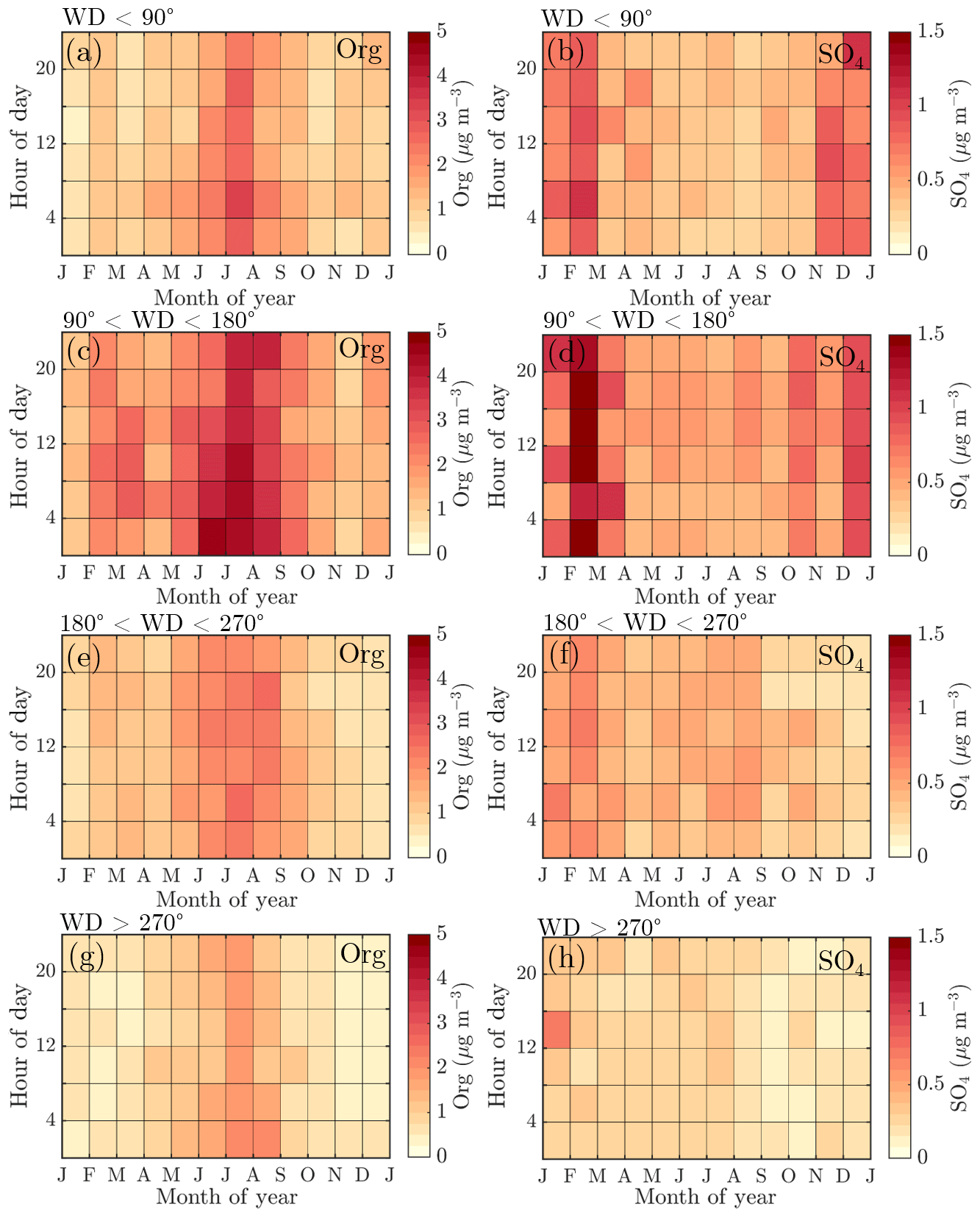
Figure 8 Diurnal cycles of organic aerosol and sulfate divided into different wind direction bins: (a–b) wind direction <90^∘, (c–d) wind direction 90–180^∘, (e–f) wind direction 180–270^∘, and (g–h) wind direction >270^∘. The y axes represent the local time of day (UTC+2), and the x axes represent the time of the year. The color scales represent the organic aerosol and sulfate aerosol mass concentrations in µg m⁻³. Figure A1 introduces the likelihoods of each wind direction bin via a traditional wind rose plot.

The highest organic aerosol loading was observed during summer for all of the wind direction bins (I–IV) with rather modest diurnal variability, perhaps due to the coarse time resolution used (Fig. 8a, c, e, g). The greatest organic aerosol concentration was associated with sector II that covers the direction of the Korkeakoski sawmills located 6–7 km to the SE (Fig. 8c). Moreover, the February peak in organic aerosol was also most distinguishable from sector II (Fig. 8c). Sulfate aerosol in turn was mostly detected with winds from sector I and II (Fig. 8b, d, f, h). Sector I shows a general wintertime enhancement (Fig. 8b), whereas sector II shows a clear maximum during February (Fig. 8d). The westerly sectors (III and IV) were associated with cleaner air (Fig. 8e–h).

3.3.2 Openair: organics and monoterpenes

Finally, we investigate the aerosol chemical composition dependence of wind speed and direction utilizing openair polar plots. As the polar plots do not take into account the frequency of certain wind direction and speed combinations, Figs. 1c–d and A1 are important when drawing conclusions based on them.

Organic aerosol concentration at SMEAR II increased with SE–S winds, as already visualized in Fig. 8c (Fig. 9a). The monoterpene mixing ratio also peaked, with a more narrow range of wind directions, analogous with the direction of the nearby Korkeakoski sawmills (Fig. 9d). With higher wind speeds, monoterpenes were also observed from a wider span of wind directions. Organic aerosol showed wind speed dependence with SE–S winds, with lower concentrations associated with wind speed exceeding 25 km h⁻¹ (ca. 6.9 m s⁻¹). A possible explanation is that the monoterpene emissions from the sawmills did not have time to oxidize and form SOA with such high wind speeds before reaching SMEAR II. Organic aerosol concentration was relatively constant outside the sawmill interference, though the lowest loadings were detected when air masses arrived with wind speeds exceeding 20 km h⁻¹ (ca. 5.5 m s⁻¹) from the NW sector. In contrast, monoterpene mixing ratio was rather constant with varying wind directions and wind speeds, except for from the direction of the sawmills (approximately 130^∘). Similar observations of the wind direction dependence of monoterpene mixing ratios have been reported before, with a subsequent organic aerosol mass concentration increase at SMEAR II with SW winds (Eerdekens et al., 2009; Liao et al., 2011).

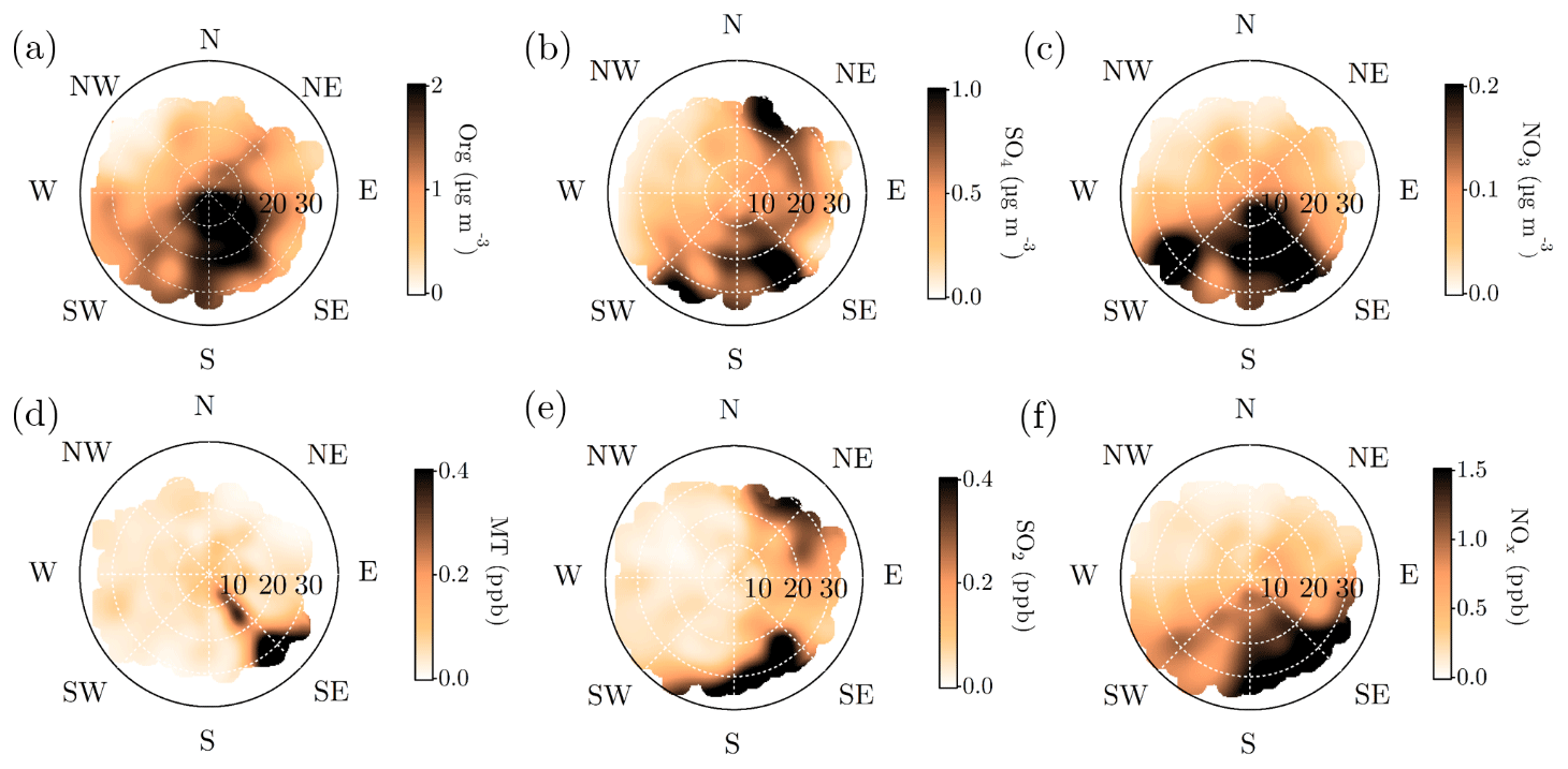
Figure 9 Openair polar plots for organic aerosol (a), sulfate (b), nitrate (c), monoterpenes (d), SO₂ (e), and NO_x (f). The distances from the origin indicates wind speeds in km h⁻¹. The wind speed grid lines are presented with dashed white circles. The color scales represent the concentrations observed with each wind speed and direction combination. As the figures do not indicate any likelihood of the wind speed and distance combinations, Fig. A1 is important to keep in mind while interpreting them. Briefly, N–NE–E is the least probable wind direction, whereas S–SW–W is the most likely. Wind speeds generally stay below 20 km h⁻¹.

A simplified seasonal analysis on aerosol chemical composition wind dependence was performed by investigating the openair polar plots for all data recorded in February (Fig. A8) and July (Fig. A9). Korkeakoski sawmills represented the main monoterpene source in February, as the concentration coinciding with air masses arriving from other directions was negligible (Fig. A8d). In February, the sawmill emissions did not significantly enhance the organic aerosol concentration at the site, due to low oxidation rates (monoterpene lifetime up to 10 h; Peräkylä et al., 2014) and higher wind speeds (Fig. A8a). The organic aerosol concentration approached zero with NW winds during February regardless of the wind speed. A major wind speed influence can be observed with SW winds, as higher wind speeds coincide with elevated organic loading.

In July, the monoterpene mixing ratio increased regardless of the wind direction due to increased biogenic emissions from the surrounding forest, but the sawmill influence also remained elevated (Fig. A9d). The monoterpene lifetime in July is roughly 2 h (Peräkylä et al., 2014) indicating an efficient photochemical sink. Thus, monoterpene sources are likely not that far. The organic aerosol concentration was clearly overall elevated; however, the overall easterly interference was more pronounced compared to February (Fig. A9a). It could be linked to the high-pressure systems often associated with easterly winds that bring warm air and clear sky conditions to SMEAR II promoting BVOC emissions and SOA formation, as discussed earlier in the paper.

3.3.3 Openair: sulfate and SO₂

Relatively high concentrations of sulfate aerosols and sulfur dioxide were detected with N-NE and SE–SW winds (Fig. 9b and e). Riuttanen et al. (2013) performed a HYSPLIT trajectory analysis for SMEAR II for 1996–2008 with SO₂ concentration fields showing similar results. They attribute the detected SO₂ to anthropogenic emission sources in St. Petersburg, the Baltic region, the Kola Peninsula, and the SE corner of the White Sea. In addition to the major emission sources introduced by Riuttanen et al. (2013), the paper and pulp industry is a major known SO₂ emitter. Several paper and pulp mills are situated in Finland, mostly NE and SE of SMEAR II (Metsäteollisuus, 2018). Another national major SO₂ source is certainly the Kilpilahti (Porvoo) oil refinery, located ∼200 km SE–S of SMEAR II. This area represents the most extensive oil refinery and chemical industry in the Nordic countries, and the SO₂ concentrations measured downwind from the area have been close to those obtained from Kola Peninsula outflow (Sarnela et al., 2015).

Large emission sources located SW of SMEAR II listed by EMEP (European Monitoring and Evaluation Programme) did not stand out in the analysis performed by Riuttanen et al. (2013), but a wind direction dependence is visible in the current study, associated only with high wind speeds. Similar wind speed dependence was observed with SE–S and N–NE winds, as the concentration of sulfate and SO₂ clearly increased when wind speeds exceeded 20 km h⁻¹ (ca. 5.5 m s⁻¹). Such wind speed dependence can be observed with long-range transported air pollutants: their transport is generally more efficient with higher wind speeds. The results presented here are also consistent with hygroscopicity measurements conducted at SMEAR II (Petäjä et al., 2005), where the hygroscopic growth factor was greatest when SO₂-rich air arrived fast to the station from the NE.

NE and SE represented the major SO₂ sources in February. The NE SO₂ was detected with lower wind speed dependence than generally observed (Fig. A8b and e). The lifetime of SO₂ is dependent on wet and dry deposition, and oxidation to sulfate (photochemistry or aqueous-phase chemistry in cloud droplets). These factors influence the likelihood of detecting SO₂ from distant sources. The higher wintertime concentrations are also linked to the atmospheric boundary layer dynamics, as discussed earlier. The SW and SE–S winds with wind speeds exceeding 16 km h⁻¹ (ca. 4.4 m s⁻¹) were associated with sulfate during February (Fig. A8b). Sulfate was also detected with a wide range of wind directions during low wind speeds. In the case of low wind speeds, it is hard to determine the wind direction accurately. However, it was clear that sulfate was not associated with W-NW winds, as shown previously in the paper (Fig. 8b, d, f, h).

The sulfate openair polar plot for July (Fig. A9b) reveals that the sulfate transport was more wind speed dependent than in February. Moreover, the wind directions linked to sulfate presence at SMEAR II were NW-N, NE, and E–SE but observed only when the wind speeds exceeded 16 km h⁻¹ (ca. 4.4 m s⁻¹). SO₂ was only observed with wind speeds exceeded 16 km h⁻¹ (ca. 4.4 m s⁻¹) with NE winds (Fig. A9e). High wind speeds are needed in July to transport rather short-lived pollutants, such as SO₂, to SMEAR II from distant sources.

As can be seen from Figs. 9e, A8e, and A9e, elevated SO₂ concentrations (dark areas in the concentration fields) are associated with very specific, rather narrow, ranges of easterly (mainly NE and SE) wind directions and elevated wind speeds (>16–20 km h⁻¹). These figures illustrate the sensitivity of the recorded SO₂ concentration towards even moderate wind direction and speed variations. As wind direction and speed can vary significantly on an inter-annual scale, inter-annual variability in SO₂ concentration can also be expected. This could finally explain the SO₂ inter-annual variability highlighted especially in winter months (Fig. 4e). Such strong variability is not reflected further on the sulfate aerosol (Fig. 4b) year-to-year scales due to its long lifetime and build-up in the atmosphere.

3.3.4 Openair: nitrate and NO_x

The nitrate concentration field visualized in Fig. 9c was highest when the wind direction was between SE and SW. No wind speed dependence could be attributed to the nitrate associated with SE–S, whereas for SW nitrate concentration clearly elevated when wind speed exceeded 20 km h⁻¹ (ca. 5.5 m s⁻¹). NO_x concentration, in turn, was not significantly elevated with SW winds regardless of the wind speed but shows similar behavior to nitrate with SE–S winds (Fig. 9f). The nitrates arriving with SW wind likely spend more time in the atmosphere than in the case of SE–S source. A previous study focusing on organic nitrates at SMEAR II linked their occurrence to SE winds (Kortelainen et al., 2017). They suggest nighttime nitrate radical oxidation of sawmill BVOCs as their major source. The same study attributes inorganic ammonium nitrate with SW winds. The study was conducted in springtime. Also our results suggested an increased organic nitrate presence in spring compared to wintertime (Fig. 7g).

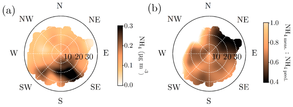
Figure 10 Openair polar plots for ammonium (a) and the ratio between measured and predicted ammonium (b). The distances from the origin indicates wind speeds in km h⁻¹. The wind speed grid lines are presented with dashed white circles. The color scales represent the concentration (a) and the unitless ammonium ion balance ratio (b) observed with each wind speed and direction combination. As the figures do not indicate any likelihood of the wind speed and distance combinations, Fig. A1 is important to keep in mind while interpreting them. Briefly, N–NE–E is the least probable wind direction, whereas S–SW–W is the most likely. Wind speeds generally stay below 20 km h⁻¹.

In February, the nitrate concentration field resembles the overall concentration field depicted in Fig. 9c, but the highest loadings were typically associated with low wind speeds from SE–S (Fig. A8c). The reason for not observing nitrate with high wind speeds could be the fact that there is not enough time for nitrate aerosol formation. NO_x concentration was overall elevated between NE and SE, and the clean NW–S sector had negligible NO_x loading (Fig. A8f). Despite the NO_x availability in the north, no nitrate aerosol was observed. This could be due to limited ammonia availability in wintertime. Most NO_x was detected with E–SE winds when wind speed was 8–16 km h⁻¹ (ca. 2.2–4.4 m s⁻¹).

In July, SW winds blew most of the nitrate to SMEAR II (Fig. A9c). However, slightly elevated concentrations can also be observed with SE–E winds (Fig. A9c). The nitrate associated with SW winds again requires high wind speeds. The NO_x concentration was significantly lower in July compared to February, as already shown in Fig. 4f (Fig. A9f). No clear wind speed dependence was observed.

3.3.5 Openair: ammonium and ion balance

The overall polar plot for ammonium, visualized in Fig. 10a, did not show elevated abundance with N-NE winds in contrast to sulfate polar plot (Fig. 9b). Moreover, the ammonium ion balance showed the lowest values with the N–NE winds that often carry the sulfate-rich aerosols to SMEAR II (Figs. 9b and 10b). Such observations hint towards acidic aerosols. Riva et al. (2019) observed acidic aerosols likely originating from the Kola Peninsula that support this hypothesis. Moreover, the particle acidity further drove chemical transformations in the aerosol organic leading to a higher presence of oligomers in the aerosol. The hygroscopicity analysis carried out at SMEAR II back in 2005 also showed how the particles arriving from NE were the most hygroscopic (Petäjä et al., 2005), which is a property boosted in acidic aerosols. The clean NW sector shows bright values for the ammonium balance field. Here, the ammonium balance exceeds 1, due to the noisiness of the data introduced by both ammonium and nitrate used in the ammonium balance calculation being below their detection limits during NW winds.

4 Conclusions

To better understand the boreal forest aerosol, an aerosol chemical speciation monitor (ACSM) was installed for long-term monitoring of sub-micrometer aerosol chemical composition in 2012 at the research site of SMEAR II. The measurements continue to this day. Such measurements at the site had been previously conducted only in short-term intensive measurement campaigns, leaving our understanding of the seasonal and year-to-year variability lacking. The current study spans over the first seven years (2012–2018) of online monitoring of the sub-micrometer non-refractory aerosol composition, finally providing this missing piece in SMEAR II aerosol documentation.

The median mass concentration over the measurement period was 2.3 µg m⁻³ (1.2 and 4.0 µg m⁻³ for the 25th and 75th percentiles, respectively) of which 68 % was organics, 20 % was sulfate, 6 % was nitrate, and 6 % was ammonium. Chloride concentrations in the non-refractory sub-micrometer particles were negligible (<1 %). As many factors, such as ambient temperature, solar radiation, atmospheric boundary layer height, and wind influence the aerosol particle concentrations and trace gas emissions, oxidation, and volatility, we observed a clear seasonal cycle in NR-PM₁ loading and composition.

During warm months, biogenic VOC emissions increase and upon oxidation produce SOA, which represents a major source of PM at SMEAR II. Organic aerosol mass concentration achieved its annual maximum in July (3.3, 1.7, and 4.6 µg m⁻³ for the median, 25th, and 75th percentiles, respectively) that further lead to the annual maximum in the total NR-PM₁ loading (4.2, 2.2, and 5.7 µg m⁻³ for the median, 25th, and 75th percentiles, respectively). Organics on average made up 80 % of the NR-PM₁ in summer. During the exceptionally hot months of July of 2014 and 2018, the organic aerosol concentrations were up to 70 % higher than the 7-year July mean. Most of the mass could be associated with increased biogenic SOA production. The projected increase in heat wave frequency over Finland (and in general) will most likely influence the loading and chemical composition of aerosol particles, and subsequently affect the Earth's radiative balance. Also from this perspective, continuing the long-term measurements at SMEAR II is essential.

Winter months indicate low amounts of solar radiation and a shallow boundary layer. NO_x and SO₂, the main precursors for particulate nitrate and sulfate, respectively, achieved their maximum mixing ratios during the darkest months while emitted into the shallow boundary layer during the period of low photochemical activity. These species are generally emitted in combustion processes that lead to high wintertime concentrations both due to the additional need of residential heating as well as the shallow boundary layer prohibiting their vertical mixing. The maximum wintertime NR-PM₁ concentration was most commonly detected in February, and explained by an enhancement of inorganic aerosol species. The particulate sulfate and nitrate peaked in February, which was later than their precursors, as a combined result of wind patterns, deposition mechanisms and photochemistry affecting their formation and removal rates. The contribution of inorganic aerosol species was ca. 50 % of the total NR-PM₁ (2.7, 1.6, 5.1 µg m⁻³ for the median, 25th, and 75th percentiles, respectively) in February, of which 30 % was sulfate, 10 % was nitrate, and 10 % was ammonium. Importantly, much of these inorganic aerosol species were most likely from long-range transport. If emission regulations regarding SO₂ and NO_x become stricter in the future in Europe, especially in Russia, the wintertime NR-PM₁ might decrease significantly at SMEAR II.

In our understanding, this is the longest time series reported describing the aerosol chemical composition measured online in the boreal region. Long-term monitoring of changes introduced by emission regulations, together with the changes introduced by the changing climate, are crucial for understanding the aerosol sensitivity of the (boreal) climate. Thus, we will keep the ACSM measurements going at SMEAR II to obtain an even longer data set. The data presented here will be publicly available, and we welcome collaborative work in utilizing this information for broadening the understanding of the boreal environment.

Appendix A: Supporting figures

Figure A1 Wind rose diagrams during the overall measurement period (a), February (b), and July (c). The distance from origin reflects the likelihood of each direction (%) and the color scale reflects the likelihoods of different wind speeds associated with the direction.

Figure A2 Data availability during the measurement period. The instrument and measurement parameter is on the y axis, and time is on the x axis. Gaps in the red line correspond to times when no data were available.

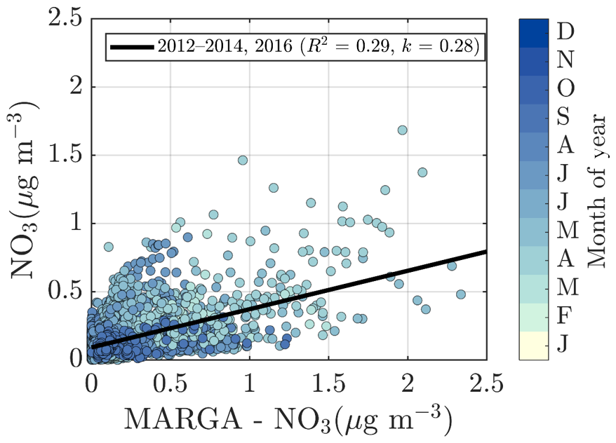
Figure A3 The ACSM nitrate vs. the PM_2.5 nitrate detected with MARGA-2S. The color coding represents the month of the year. The black line represents the overall linear fit.

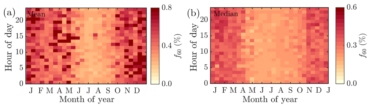
Figure A4 The mean (a) and median (b) f₆₀ (the fraction of m∕Q 60 Th signal of the total OA signal) values derived from the ACSM measurements (2012–2018 at SMEAR II). The x axes represent the time of the year and the y axes the hour of the day (UTC+2). The colored pixels represent the f₆₀ values. Note the different color scales between the mean and median figures. It is also worth mentioning that due to the rather low signal to noise ratio of the ACSM, the f₆₀ estimates can be very noisy. To avoid the weight of the high and low noise extremes in (a) (mean f₆₀), only the range of $\mathrm{0}\ge f_{\mathrm{60}}\le \mathrm{1}$ were included in the f₆₀ mean field calculation.

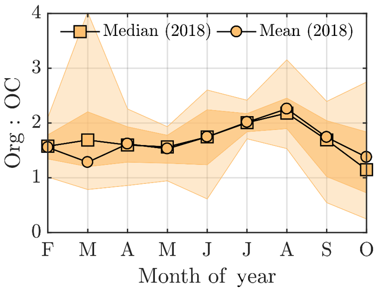
Figure A5 Organic carbon concentration (OC) vs. the organic aerosol concentration (Org) in 2018 at SMEAR II. The darker yellow shadings indicate the area between the 25th and 75th percentiles and the lighter yellow shadings indicate the area between the 10th and 90th percentiles.

Figure A6 (a) Average SO₂ concentration in the atmospheric column derived from the ozone monitoring instrument (OMI) aboard Aura satellite for September 2014. High values near Iceland are due to the 2014–2015 flood lava eruption of the Bárðarbunga volcano. (b) A 2-D normalized histogram of air parcel back trajectories arriving at the SMEAR II station for September 2014. The trajectories are computed using the HYSPLIT model going back 96 h in time with a resolution of nine arriving trajectories per hour. Each air parcel path is recorded for each hour. These points are binned in 2×2^∘ cells. The counting of each cell is then normalized by multiplying it with the square of the distance to the SMEAR II station (black disk marker) in order to highlight the long-range transport patterns.

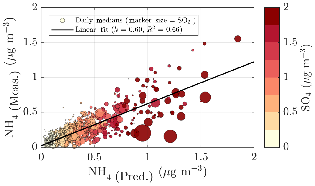
Figure A7 The relationship between the measured and predicted ammonium concentrations. The marker size reflects the ambient SO₂ concentration and the color scale sulfate concentration. The linear fit represents the ratio between the measured and predicted ammonium concentration. Drifting from 1 could be linked to more basic or acidic aerosols. The linear fit of 0.66 indicates a possibility of acidic aerosols that decreases in the presence of SO₂. A better acidity approximation could be derived with thermodynamical models.

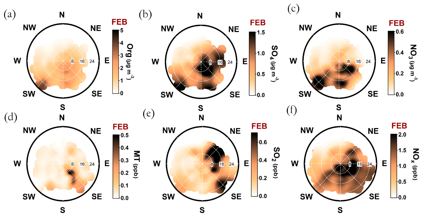
Figure A8 Openair polar plots for organic aerosol (a), sulfate (b), nitrate (c), monoterpenes (d), SO₂ (e), and NO_x (f) during February. The distance from the origin indicates wind speeds in km h⁻¹. The wind speed grid lines are presented with dashed white circles. The color scales represent the concentrations observed with each wind speed and direction combinations. As the figures do not indicate any likelihood of the wind speed and distance combinations, Fig. A1 is important to keep in mind while interpreting them. Briefly, N–NE–E is the least probable wind direction, whereas S–SW–W is the most likely. Wind speeds generally stay below 20 km h⁻¹.

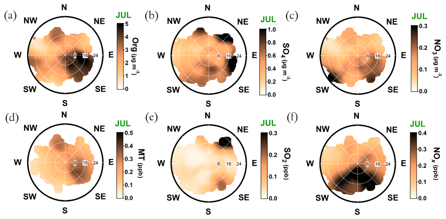
Figure A9 Openair polar plots for organic aerosol (a), sulfate (b), nitrate (c), monoterpenes (d), SO₂ (e), and NO_x (f) during July. The distance from the origin indicates wind speeds in km h⁻¹. The wind speed grid lines are presented with dashed white circles. The color scales represent the concentrations observed with each wind speed and direction combinations. As the figures do not indicate any likelihood of the wind speed and distance combinations, Fig. A1 is important to keep in mind while interpreting them. Briefly, N–NE–E is the least probable wind direction, whereas S–SW–W is the most likely. Wind speeds generally stay below 20 km h⁻¹.