the Creative Commons Attribution 4.0 License.
the Creative Commons Attribution 4.0 License.
 | 14 Feb 2020
Uncertainty analysis of a European high-resolution emission inventory of CO2 and CO to support inverse modelling and network design
Stijn N. C. Dellaert
Antoon J. H. Visschedijk
Hugo A. C. Denier van der Gon
Quantification of greenhouse gas emissions is receiving a lot of attention because of its relevance for climate mitigation. Complementary to official reported bottom-up emission inventories, quantification can be done with an inverse modelling framework, combining atmospheric transport models, prior gridded emission inventories and a network of atmospheric observations to optimize the emission inventories. An important aspect of such a method is a correct quantification of the uncertainties in all aspects of the modelling framework. The uncertainties in gridded emission inventories are, however, not systematically analysed. In this work, a statistically coherent method is used to quantify the uncertainties in a high-resolution gridded emission inventory of CO2 and CO for Europe. We perform a range of Monte Carlo simulations to determine the effect of uncertainties in different inventory components, including the spatial and temporal distribution, on the uncertainty in total emissions and the resulting atmospheric mixing ratios. We find that the uncertainties in the total emissions for the selected domain are 1 % for CO2 and 6 % for CO. Introducing spatial disaggregation causes a significant increase in the uncertainty of up to 40 % for CO2 and 70 % for CO for specific grid cells. Using gridded uncertainties, specific regions can be defined that have the largest uncertainty in emissions and are thus an interesting target for inverse modellers. However, the largest sectors are usually the best-constrained ones (low relative uncertainty), so the absolute uncertainty is the best indicator for this. With this knowledge, areas can be identified that are most sensitive to the largest emission uncertainties, which supports network design.
- Article
(9053 KB) - Full-text XML
- BibTeX
- EndNote


Carbon dioxide (CO2) is the most abundant greenhouse gas and is emitted in large quantities from human activities, especially from the burning of fossil fuels (Berner, 2003). A reliable inventory of fossil fuel CO2 (FFCO2) emissions is important to increase our understanding of the carbon cycle and how the global climate will develop in the future. The impact of CO2 emissions is visible on a global scale and international efforts are required to mitigate climate change, but cities are the largest contributors to FFCO2 emissions (about 70 %, IEA, 2008). Therefore, emissions should be studied at different spatial and temporal scales to get a full understanding of their variability and mitigation potential.
One way of describing emissions is an emission inventory, which is a structured set of emission data, distinguishing different pollutants and source categories. Often, emission inventories are based on reported emission data, for example, from the National Inventory Reports (NIRs) (UNFCCC, 2019), which are national, yearly emissions based on energy statistics. These country-level emissions can be spatially and temporally disaggregated (scaled-down) to a certain level using proxies (e.g. the inventories of the Netherlands Organisation for Applied Scientific Research (TNO); Denier van der Gon et al., 2017; Kuenen et al., 2014). Other emission inventories are based on local energy consumption data and reported emissions, which are (dis)aggregated to the required spatial scale (e.g. Hestia, Gurney et al., 2011, 2019) or rely on (global) statistical data and a consistent set of (non-country-specific) emission factors representing different technology levels, e.g. Emissions Database for Global Atmospheric Research (EDGAR) (http://edgar.jrc.ec.europa.eu, last access: 6 May 2019). Most inventories, including the one used in this study, rely on a combination of methods, using large-scale data supplemented with local data. Gridded emission inventories are essential as input for atmospheric transport models to facilitate comparison with observations of CO2 concentrations, as well as in inverse modelling as a prior estimate of the emission locations and magnitude.
During the compilation of an emission inventory, uncertainties are introduced at different levels (e.g. magnitude, timing or locations), and increasingly more attention is given to this topic. Parties of the United Nations Framework Convention on Climate Change (UNFCCC) report their annual emissions (disaggregated over source sectors and fuel types) in a NIR (UNFCCC, 2019), which includes an assessment of the uncertainties in the underlying data and an analysis of the uncertainties in the total emissions following IPCC (Intergovernmental Panel on Climate Change) guidelines. The simplest uncertainty analysis is based on simple equations for combining uncertainties from different sources (Tier 1 approach). A more advanced approach is a Monte Carlo simulation, which allows for non-normal uncertainty distributions (Tier 2 approach). The Tier 2 approach has been used by several countries, for example, Finland (Monni et al., 2004) and Denmark (Fauser et al., 2011).
These reports provide a good first step in quantifying emission uncertainties, but the uncertainty introduced by using proxies for spatial and temporal disaggregation is not considered. These are, however, an important source of uncertainty in the gridded emission inventories (Andres et al., 2016). Inverse modelling studies are increasingly focusing on urban areas, the main source areas of FFCO2 emissions, for which emission inventories with a high spatiotemporal resolution are used to better represent the variability in local emissions affecting local concentration measurements. Understanding the uncertainty at higher resolution than the country level is thus necessary, which means that the uncertainty caused by spatiotemporal disaggregation becomes important as well.
The uncertainties in emission inventories are important to understand for several reasons. First, knowledge of uncertainties helps to pinpoint emission sources or areas that require more scrutiny (Monni et al., 2004; Palmer et al., 2018). Second, knowledge of uncertainties in prior emission estimates is an important part of inverse modelling frameworks, which can be used for emission verification and in support of decision-making (Andres et al., 2014). For example, if uncertainties are not properly considered, there is a risk that the uncertainty range does not contain the actual emission value. In contrast, if uncertainties are overestimated, the initial emission inventory gives little information about the actual emissions and more independent observations are needed. Third, local inverse modelling studies often rely on daytime (12:00–16:00 LT) observations, which are easier to simulate. Given the small size of the urban domain, these observations only contain information on recent emissions, which have to be extrapolated using temporal profiles to calculate annual emissions. Therefore, knowledge of uncertainties in temporal profiles helps to better quantify the uncertainty in these annual emissions. Finally, emission uncertainties can support atmospheric observation system design, for example, for inverse modelling studies. An ensemble of model runs can represent the spread in atmospheric concentration fields due to the uncertainty in emissions. Locations with a large spread in atmospheric concentrations are most sensitive to uncertainties in the emission inventory and are preferential locations for additional atmospheric measurements. To conclude, emission uncertainties are a critical part of emission verification systems and require more attention. To better understand how uncertainties in underlying data affect the overall uncertainty in gridded emissions, a family of 10 emission inventories is compiled within the CO2 Human Emissions (CHE) project, which is funded by the Horizon 2020 EU Research and Innovation programme (see data availability). The methodology used to create this family of emission inventories also forms the basis for the work described here.
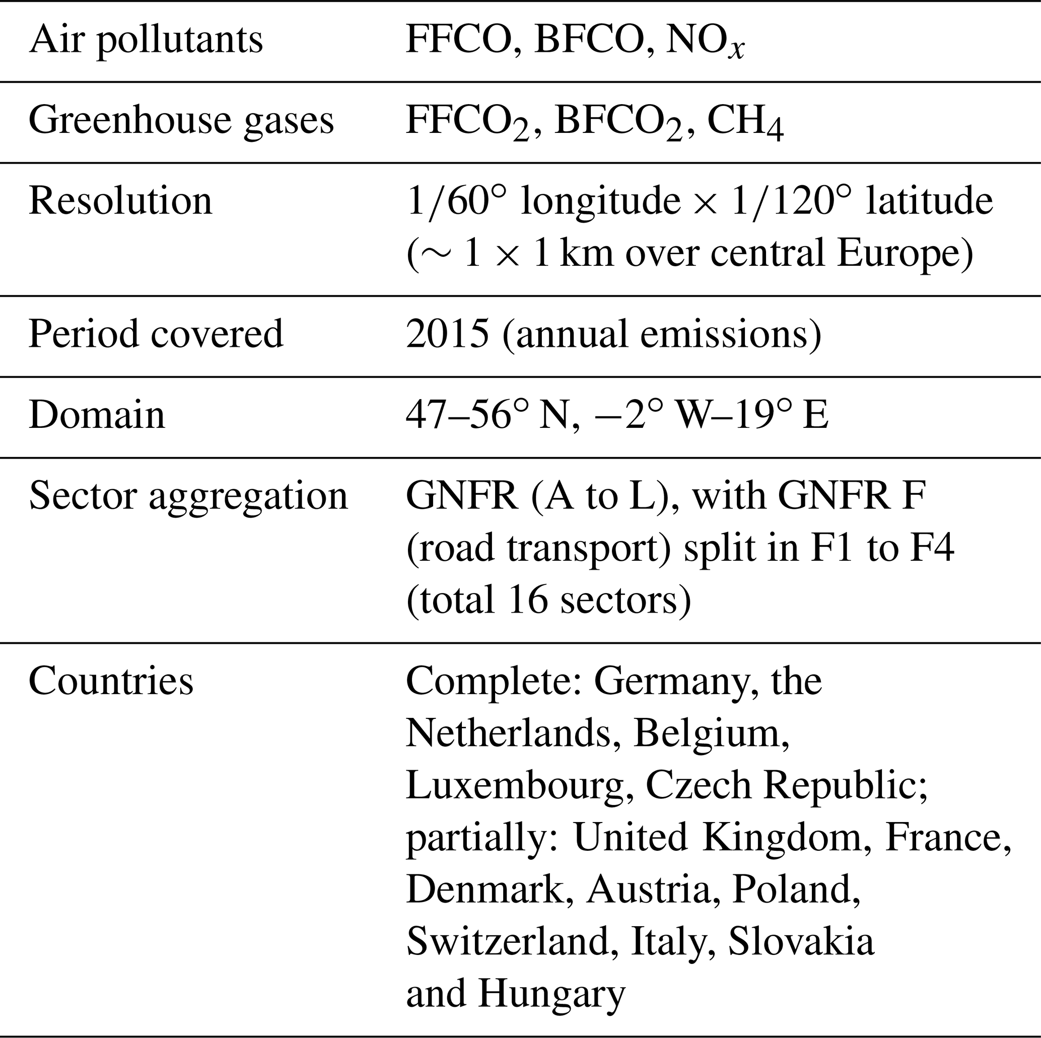
In this paper, we illustrate a statistically coherent method to assess the uncertainties in a high-resolution emission inventory, including uncertainties resulting from spatiotemporal disaggregation. For this purpose, we use a Monte Carlo simulation to propagate uncertainties in underlying parameters into the total uncertainty in emissions (like the Tier 2 approach). We illustrate our methodology using a new high-resolution emission inventory for a European region centred over the Netherlands and Germany (Table 1, Fig. 1). We illustrate the magnitude of the uncertainties in emissions and how this affects simulated concentrations. The research questions are as follows:
-
How large are uncertainties in total inventory emissions, and how does this differ per sector and country?
-
How do uncertainties in spatial proxy maps affect local measurements?
-
How important is the uncertainty in temporal profiles for the calculation of annual emissions from daytime (12:00–16:00 LT) emissions, which result from urban inverse modelling studies using only daytime observations?
-
What information can we gain from high-resolution gridded uncertainty maps by comparing different regions?
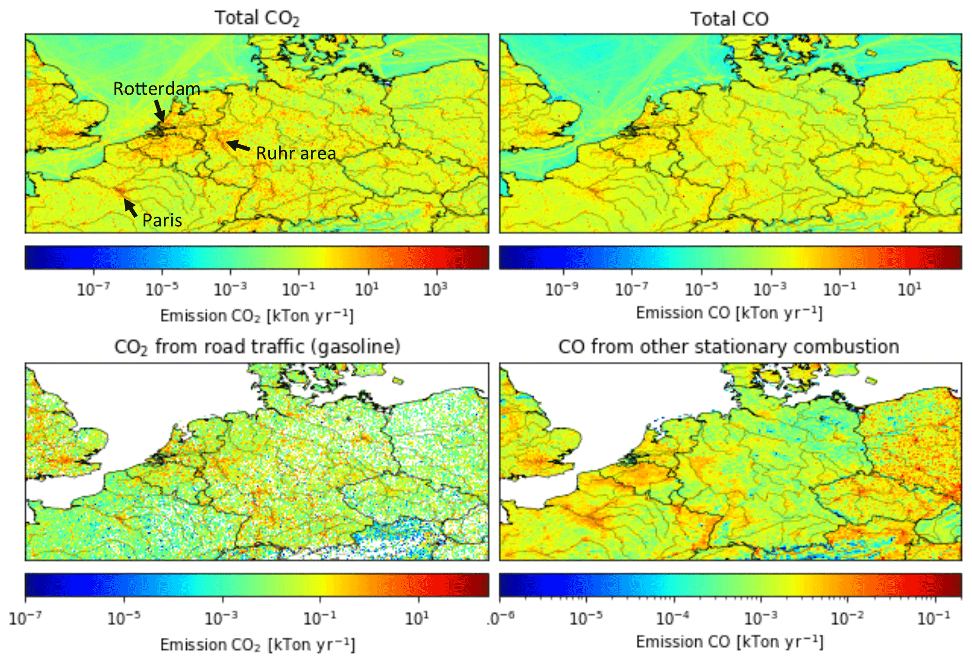
Figure 1Total emissions of CO2 and CO, road traffic (gasoline) emissions of CO2 and other stationary combustion emissions of CO for 2015 in kt yr−1 (defined per grid cell).
Inverse modelling studies often focus on a single species like CO2, but co-emitted species are increasingly included to allow source apportionment (Boschetti et al., 2018; Zheng et al., 2019). In this study, we look into CO2 and CO to illustrate our methodology, but the methodology can be applied to other (co-emitted) species.
Table 1Characteristics of the high-resolution emission inventory TNO GHGco v1.1 containing fossil fuel (FF) and biofuel (BF) emissions.
2.1 The high-resolution emission inventory
The basis of this study is a high-resolution emission inventory for the greenhouse gases CO2 and CH4 and the co-emitted tracers CO and NOx for the year 2015 (TNO GHGco v1.0; see details in Table 1). In this paper, we only use CO2 and CO, which are divided into fossil fuel (FF) and biofuel (BF) emissions (no land use and land use change emissions are included). The emission inventory covers a domain over Europe, including Germany, Netherlands, Belgium, Luxembourg and the Czech Republic, and parts of Great Britain, France, Denmark, Austria and Poland (see also Fig. 1).
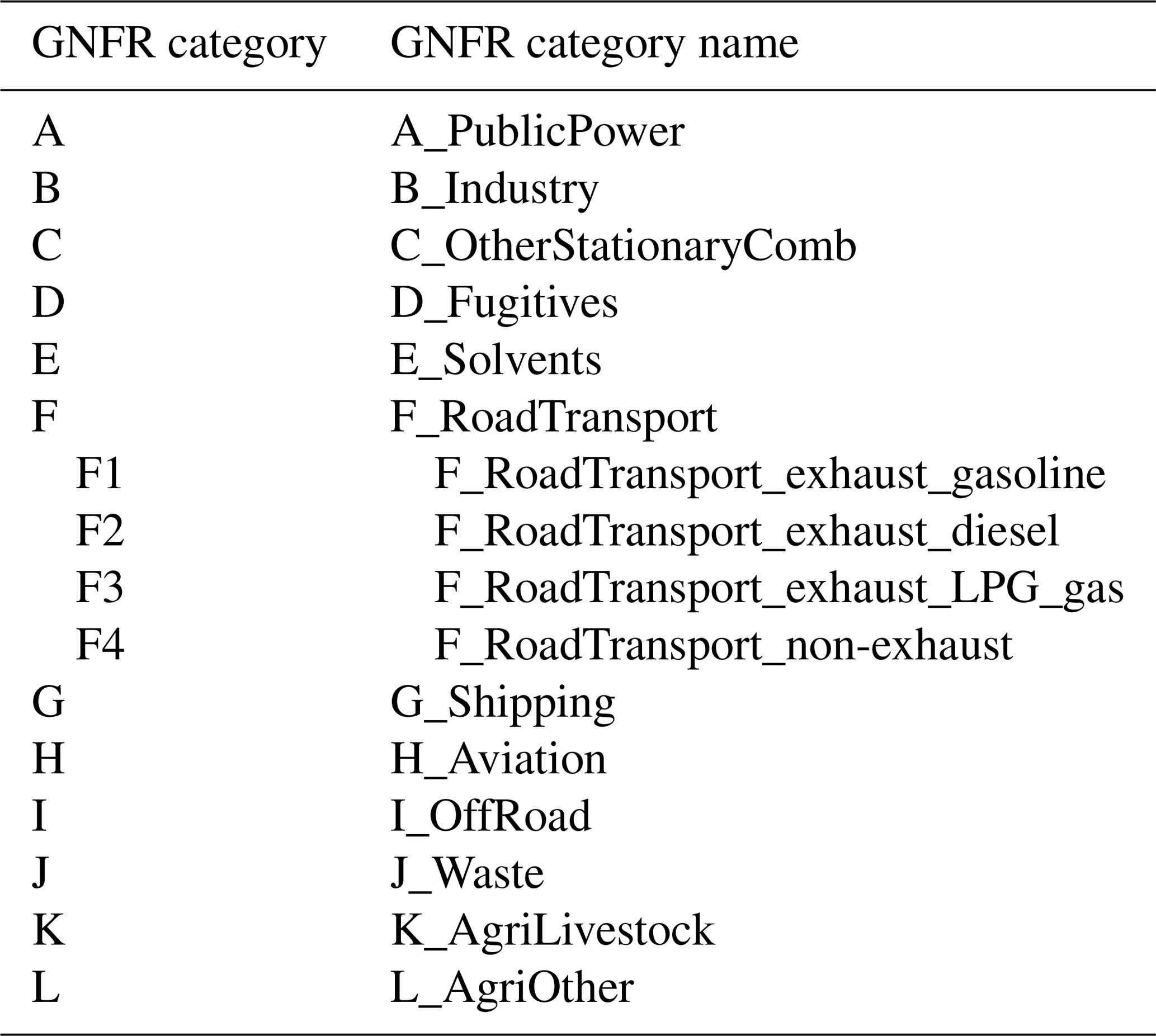
The emission inventory is based on the reported emissions by European countries to the UNFCCC (only greenhouse gases) and to EMEP/CEIP (European Monitoring and Evaluation Programme/Centre on Emission Inventories and Projections, only air pollutants). UNFCCC CO2 emissions have been aggregated to ∼250 different combinations of Nomenclature For Reporting (NFR) sectors and fuel types. EMEP/CEIP CO emissions have been split over the same NFR sector–fuel type combinations by TNO using the GAINS model (Amann et al., 2011) and/or TNO data. In some cases, the reported data were gap filled or replaced with emissions from the GAINS model, EDGAR inventory or internal TNO estimates to obtain a consistent dataset. Next, each NFR sector is linked to a high-resolution proxy map (e.g. population density for residential combustion of fossil fuels or AIS (Automatic Identification System) data for shipping regridded to ), which is used to spatially disaggregate the reported country-level emissions. Where possible, the exact location and reported emission of large point sources are used (e.g. from the European Pollutant Release and Transfer Register; E-PRTR). The third step is temporal disaggregation, for which standard temporal profiles are used (Denier van der Gon et al., 2011). Finally, the emissions are aggregated to GNFR (gridded NFR) sectors (see Table 2) for the emission inventory. The final emission maps of CO2 and CO are shown in Fig. 1, together with two examples of a source sector map. Note that these maps do not clearly show the large point source emissions, while these make up almost 45 % of all CO2 emissions and 26 % of all CO emissions.
Table 2Overview of aggregated NFR (GNFR) sectors distinguished in the emission inventory.
2.2 Uncertainties in parameters
The emission inventory is used as basis for an uncertainty analysis by assigning an uncertainty to each parameter underlying the UNFCCC-EMEP/CEIP emission inventories and further disaggregation thereof. Although the aggregation to GNFR sectors makes the emission inventory more comprehensible, we use the more detailed underlying data for the uncertainty analysis. The reason is that the uncertainties can vary enormously between subsectors and fuel types. Generally, the emission at a certain time and place is determined by four types of parameters: activity data, emission factor, spatial distribution and temporal profile. The activity data and emission factors are used by countries to calculate their emissions. The spatial proxy maps and temporal profiles are used for spatiotemporal disaggregation. All uncertainties need to be specified per NFR sector–fuel type combination that is part of the Monte Carlo simulation. In the following sections, the steps taken to arrive at a covariance matrix for the Monte Carlo simulation are described. Tables with uncertainty data can be found in Appendix A.
2.2.1 Parameter selection
The first step is to identify which parameters should be included in the Monte Carlo simulation. As mentioned before, there are about 250 different combinations of NFR sectors and fuel types, and including all of them would be a huge computational challenge. However, a selection of 112 combinations makes up most of the fossil fuel emissions (96 % for CO2 and 92 % for CO), and therefore a preselection was made. This results in a covariance matrix of 224×224 parameters (112 sector–fuel combinations for two species). To further reduce the size of the problem, the emissions are partly aggregated before starting the Monte Carlo simulation for the spatial proxies (mostly fuels are combined per sector, because they have the same spatial distribution). This results in a total of 59 NFR sector–spatial proxy combinations, which are put in a separate covariance matrix. The temporal profiles are applied to the aggregated GNFR sectors, which make up the last covariance matrix. Note that the spatial proxies and temporal profiles are the same for CO2 and CO. Only the spatially explicit E-PRTR point source data can have a different spatial distribution for CO2 and CO, but they also use the same temporal profiles.
2.2.2 Uncertainties in reported emissions
Country-level emissions are estimated from the multiplication of activity data and emission factors. Activity data consist for the most part of fossil fuel consumption data available from national energy balances. Some fuel consumptions are better known than others and uncertainties vary across sectors. An emission factor is the amount of emission that is produced per unit of activity (e.g. amount of fuel consumed). For CO2, this depends mainly on the carbon content of the fuel. In contrast, CO emissions are extremely dependent on combustion conditions, choice of industrial processes and in-place technologies.
The NIRs for greenhouse gases (GHGs) provide a table with uncertainties in activity data and CO2 emission factors on the level of NFR sector–fuel combinations. The uncertainties reported by each country are averaged to get one uncertainty per NFR sector–fuel combination for the entire domain. Overall, the differences in reported uncertainties between countries are small. The uncertainties in activity data and CO2 emission factors are relatively low and normally distributed.
The CO emission factors are mostly based on uncertainty ranges provided in the EMEP/EEA Guidebook (European Environment Agency, 2016) and supplemented by BAT reference documents from which reported emission factor ranges are taken as uncertainty range (http://eippcb.jrc.ec.europa.eu/reference/, last access: 24 January 2019). The CO emission factor uncertainties are generally expressed by a factor, which means that the highest and lowest limit values are either the specified factor above or below the most common value. Therefore, these uncertainties have a lognormal distribution and are relatively large.
To estimate the overall uncertainty in the emissions per NFR sector–fuel combination, the uncertainties in the activity data and emission factors need to be combined (shown in Fig. 2 for the aggregated GNFR sectors). When both uncertainties are of the same order and relatively small, as well as both having a normal distribution, the overall emission uncertainty is calculated with the standard formula for error propagation for non-correlated normally distributed variables (see Sect. 2.4). For most CO emission factors, uncertainties are much higher and have a lognormal distribution instead of normal. In that case, the uncertainty of the variable with the highest uncertainty is assumed to be indicative of the overall uncertainty of the emission, which in general means the uncertainty of the CO emission factor determines the overall uncertainty of the CO emission, with the distribution remaining lognormal. The error introduced by fuel type disaggregation for CO is not considered.
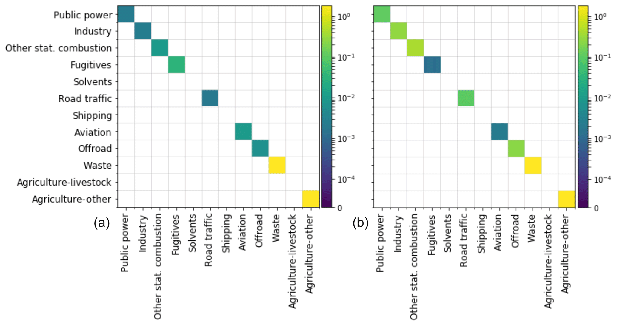
Figure 2Covariance matrices for total emissions of CO2 (a) and CO (b) per aggregated source sector. A white space on the diagonal indicates this sector is not included in the Monte Carlo simulation.
Finally, for power plants and road traffic, we assumed error correlations to exist between different subsectors per fuel type and between different fuel types per subsector for other NFR sectors. In some cases, correlations also exist between different NFR sectors belonging to the same GNFR sector. The definition of correlations is important, because they affect the total uncertainties. For example, if emission factors of subsectors are correlated, deviations can amplify each other, leading to higher overall uncertainties. In contrast, the division of the well-known total fuel consumption of a sector over its subsectors includes an uncertainty which is anti-correlated (i.e. if too much fuel consumption is assigned to one subsector, too little is assigned to another). This has little impact on the total emissions, because uncertainties only exist at lower levels.
2.2.3 Uncertainties in spatial proxies
The proxy maps used for spatial disaggregation can introduce a large uncertainty coming from the following sources:
-
The proxy is not correctly representing real-world locations of what it is supposed to represent, either because there are cells included in which none of the intended activity takes place or cells are missing in which the intended activity does take place (proxy quality).
-
The proxy is not fully representative of the activity it is assumed to represent, for example, if there is a non-linear relationship between the proxy value and the emission (proxy representativeness): a grid cell with twice the population density does not necessarily have double the amount of residential heating emissions, because heating can be more efficient in densely populated areas and/or apartment blocks.
-
The cell values themselves are uncertain, e.g. the population density or traffic intensity (proxy value).
We attempt to capture the second and third source of uncertainty in a single numerical indicator representing the uncertainty at cell level (see Fig. 3 for the uncertainty per aggregated GNFR sector). The overall uncertainties are based on expert judgement and inevitably include a considerable amount of subjectivity. This type of uncertainty is often large and has a lognormal distribution, except for proxies related to road traffic and some proxies related to commercial/residential emissions sources. We assume no error correlations exist. The first source of uncertainty is also considered in one of the experiments (see Sect. 2.4 for a description of this experiment).
2.2.4 Uncertainties in temporal profiles
For each GNFR sector, the emission timing is described using three temporal profiles: one profile that describes the seasonal cycle (monthly fractions), one profile that describes the day-to-day variations within a week (daily fractions) and one profile that describes the diurnal cycle (hourly fractions). These profiles are based on long-term average activity data and/or socioeconomic characteristics and are applied for each year and for the entire domain, considering only time zone differences. In reality, the temporal profiles can differ between countries, from year to year, and the diurnal cycle can vary between weekdays and weekends. For example, residential emissions are strongly correlated with the outside temperature, which follows a different pattern each year.
To quantify the uncertainty in temporal profiles, a range of temporal profiles (for a full year, hourly resolution) was created for each source sector based on activity data (such as traffic counts). These profiles can be from different years and countries, so that the full range of possibilities is included. These are compared to the fixed temporal profiles to estimate the uncertainties, which are normally distributed (see Fig. 3 for the uncertainty per aggregated GNFR sector). We assume no error correlations exist.
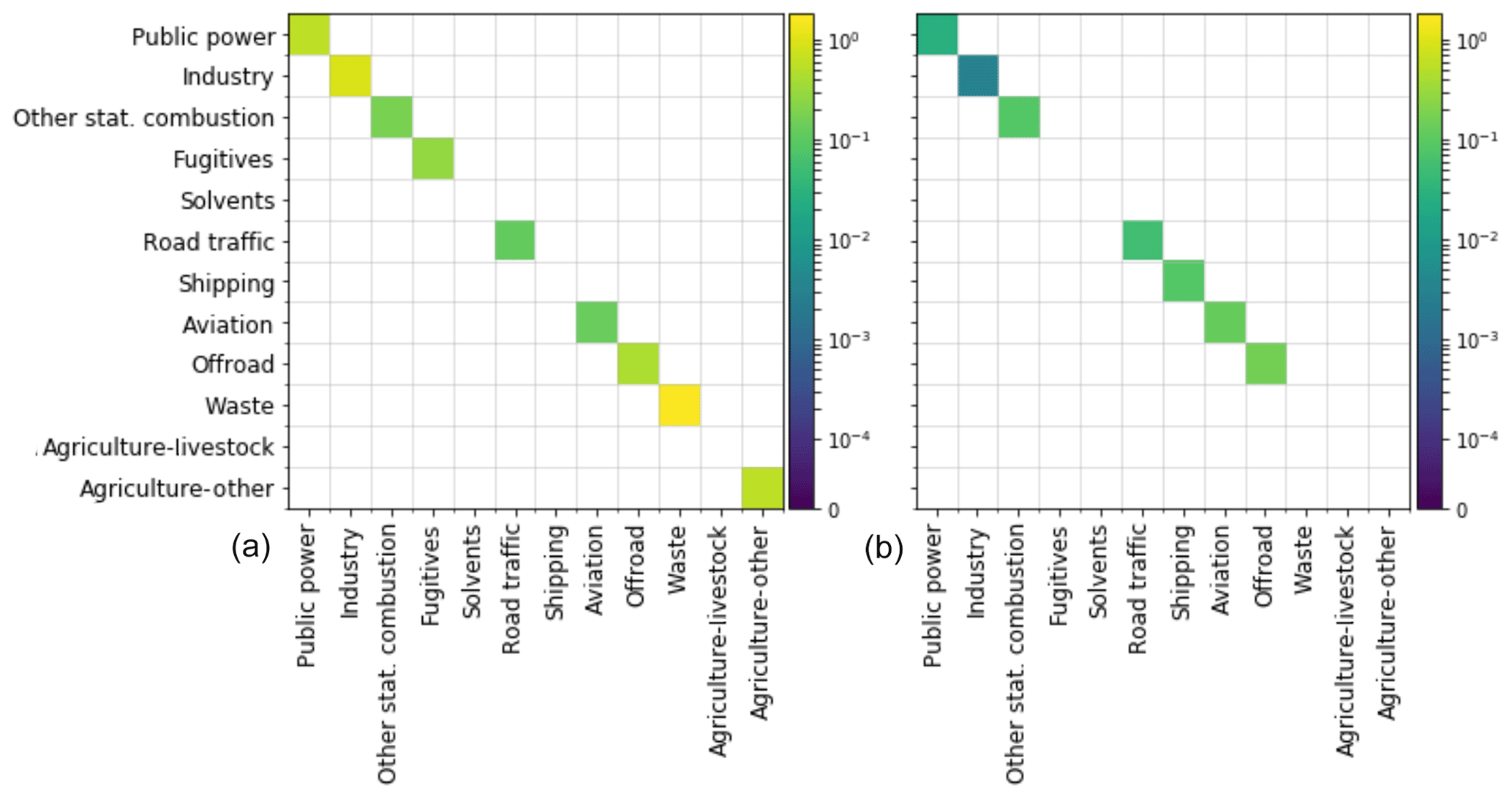
Figure 3Covariance matrices for spatial proxies (a) and time profiles (b) per aggregated source sector. These are the same for CO2 and CO. A white space on the diagonal indicates this sector is not included in the Monte Carlo simulation.
2.3 The Monte Carlo simulation
Within a Monte Carlo simulation, we create an ensemble (size N) of emissions, spatial proxies and temporal profiles by drawing random samples from the covariance matrices described in Sect. 2.2. This creates a set of possible solutions in the emission space, reflecting the uncertainties in the underlying parameters. The entire process is shown in Fig. 4. As mentioned before, not all subsectors are included in the Monte Carlo simulation and the non-included emissions are added to each ensemble member at the final stage. It is important to ensure that the temporal profiles and the spatial proxies do not affect the total emissions, so proxies should sum up to 1 for each country and temporal profiles should be on average 1 over a full year. Before doing this, negative values are removed.
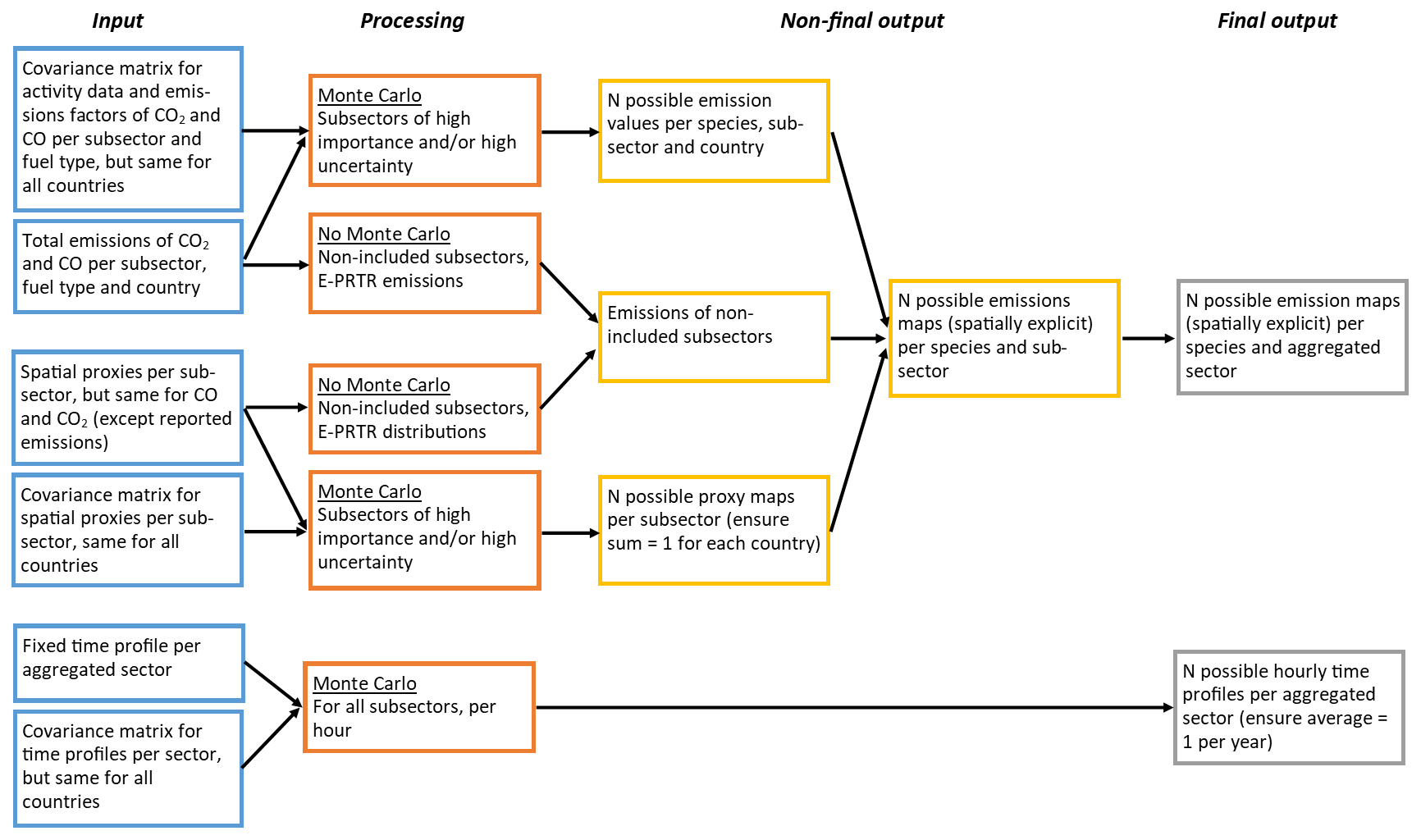
Figure 4Flow diagram showing the input, processing and output of the Monte Carlo simulation.
The source sectors that include point source emissions (mainly public power and industry) are treated separately. The large point source emissions and their locations are relatively well known and available from databases (e.g. from E-PRTR) and therefore not included in the Monte Carlo simulation. The remaining part of the emissions (non-point source or small point sources) from these sectors is distributed using generic proxies (e.g. industrial areas) and is calculated as the difference between the total emissions (activity data multiplied by the emission factor) and the sum of the point source emissions. If negative emissions result from this subtraction of reported point source emissions, the residual is set to zero. Note that the spatial uncertainty of this residual part is often high. The fractions of the public power and industrial emissions that are attributed to large point sources are shown in Table 3 for several countries.
Table 3Percentage (%) of emissions of CO2 and CO (FF plus BF) that are attributed to large point sources (accounted for in databases) for public power and industry source sectors.

2.4 Experiments to explore uncertainty propagation
In this paper, several experiments are performed to examine the impact of the uncertainties in different parameters on the overall emissions and simulated concentrations:
-
The first experiment uses a Monte Carlo simulation (N=500) to illustrate the spread in emissions per sector due to uncertainties in emission factors and activity data (no spatial/temporal variability is considered). This sample size is based on an analysis of the robustness of the uncertainty estimate (Janssen, 2013), which shows that a sample size of 500 is sufficient to get robust results (Appendix B). This experiment is used to show the contribution of specific sectors to the overall uncertainty and to illustrate how uncertainties vary between sectors and countries. For this experiment, country totals are used, also for the countries that are partially outside the zoom domain shown in Fig. 1. The results are presented in Sect. 3.1.
-
The second experiment uses a Monte Carlo simulation (N=500) to illustrate how the uncertainty in spatial proxy maps is translated into uncertainties in simulated concentrations (emissions are taken constant; no temporal variability is included). We use emissions of other stationary combustion (CO2) and road traffic (CO) to illustrate the importance of having a correct spatial distribution for measurements close to the source area and further away. The results are presented in Sect. 3.2.
-
The third experiment compares two spatial proxy maps for distributing “residual” power plant emissions (i.e. those not accounted for in point source databases) to illustrate the potential impact of spreading out small point source emissions when zooming in on small case study areas (emissions are taken constant; no temporal variability is included). The results are presented in Sect. 3.2.
-
The fourth experiment uses a Monte Carlo simulation (N=500) to illustrate the spread in temporal profiles (emissions are taken constant; no spatial variability is considered). We use this information to determine the error introduced when extrapolating daytime (12:00–16:00 LT) emissions (for example, resulting from an inversion) to annual emissions using an incorrect temporal profile. Figure 5 shows two possible daily cycles, which have 46 % (blue) and 25 % (orange) of their emissions between 12:00 and 16:00 LT. Therefore, both temporal profiles will give a different total daily emission when used to derive the daytime emissions. The results are presented in Sect. 3.3.
-
For the final experiment, maps are made of the (absolute and relative) uncertainty in each pixel, including uncertainties in emission factors, activity data and spatial proxies (no temporal variability). For this, we used a Tier 1 approach, using the following equations:
for the summation of uncorrelated quantities (e.g. sectoral emissions) and
for the multiplication of random variables, such as used to combine activity data and emission factors. Here, the (total) relative uncertainty is the percentage uncertainty (uncertainty divided by the total) and the standard deviations are expressed in units of the uncertain quantity (percentage uncertainty multiplied with the uncertain quantity). These maps are used to explore spatial patterns in uncertainties and examine what we can learn about different countries or regions. The results are presented in Sect. 3.4.
For experiments 2 and 3, a smaller domain is selected to represent a local case study (Fig. 6). We used the Rotterdam area, which has been studied in detail before (Super et al., 2017a, b). The domain is about 34×26 km and centred over the city, which includes some major industrial activity as well. To translate the emissions into atmospheric concentrations, a simple plume dispersion model is used, the Operational Priority Substances (OPS) model. This model was developed to calculate the transport of pollutants, including chemical transformations (Van Jaarsveld, 2004; Sauter et al., 2016) and was adapted to include CO and CO2 (Super et al., 2017a). The short-term version of the model calculates hourly concentrations at specific receptor points, considering hourly variations in wind direction and other transport parameters. Although the model is often used for point source emissions, it can also handle surface area sources. This model was chosen because of its very short runtime, which makes it suitable for a large ensemble. The model is run for each of the alternative emission maps.

Figure 5Schematic overview of two possible temporal profiles, which represent a different fraction of the total daily emissions during the selected period (12:00–16:00 LT, illustrated by the dashed lines).

Figure 6Emissions of CO2 (a) and CO (b) for part of the Netherlands, including the subdomain (black rectangle) over Rotterdam. Black stars indicate the receptor locations.
The OPS model is run for each ensemble member for 5 January 2014 from the start of the day until 16:00 LT. On this day, the wind direction is relatively constant at about 215∘ and the wind speed is around 6 m s−1. We specify receptor points downwind from the centre of our domain at increasing distance (5, 10, 15, 20, 30 and 40 km). We use the last hour of the simulation for our analyses. We assume emissions from other stationary combustion and road traffic (experiment 2) to take place at the surface. The initial emissions of “residual” power plants, smeared out over all industrial areas, are also emitted at the surface. However, we raise the height of the emissions to 20 m when these emissions are appointed to specific pixels. This height is representative of stack heights of small power plants.
3.1 Uncertainties in total emissions
Using the uncertainties in emission factors and activity data, we can evaluate the uncertainty in the total emissions of CO2 and CO per sector. Figure 7 shows the normalized spread in emissions per sector based on the Monte Carlo simulation (N=500). The CO2 emissions have a relatively small uncertainty range and the uncertainty in the total emissions (if we sum all GNFR sector emissions for each of the 500 solutions) is only about 1 % (standard deviation). The largest uncertainties are for fugitives and aviation, which are only small contributors to the total CO2 emissions (1.3 % and 0.4 %, respectively). Therefore, their contribution to the total emission uncertainty is very small, as is shown in Fig. 8. The largest uncertainty in the total CO2 emissions is caused by the public power sector. Despite the relatively small uncertainty in the emissions from this sector, it is the largest contributor to the total CO2 emissions (33 %), and therefore the uncertainty in the public power sector contributes about 45 % to the uncertainty in the total CO2 emissions.
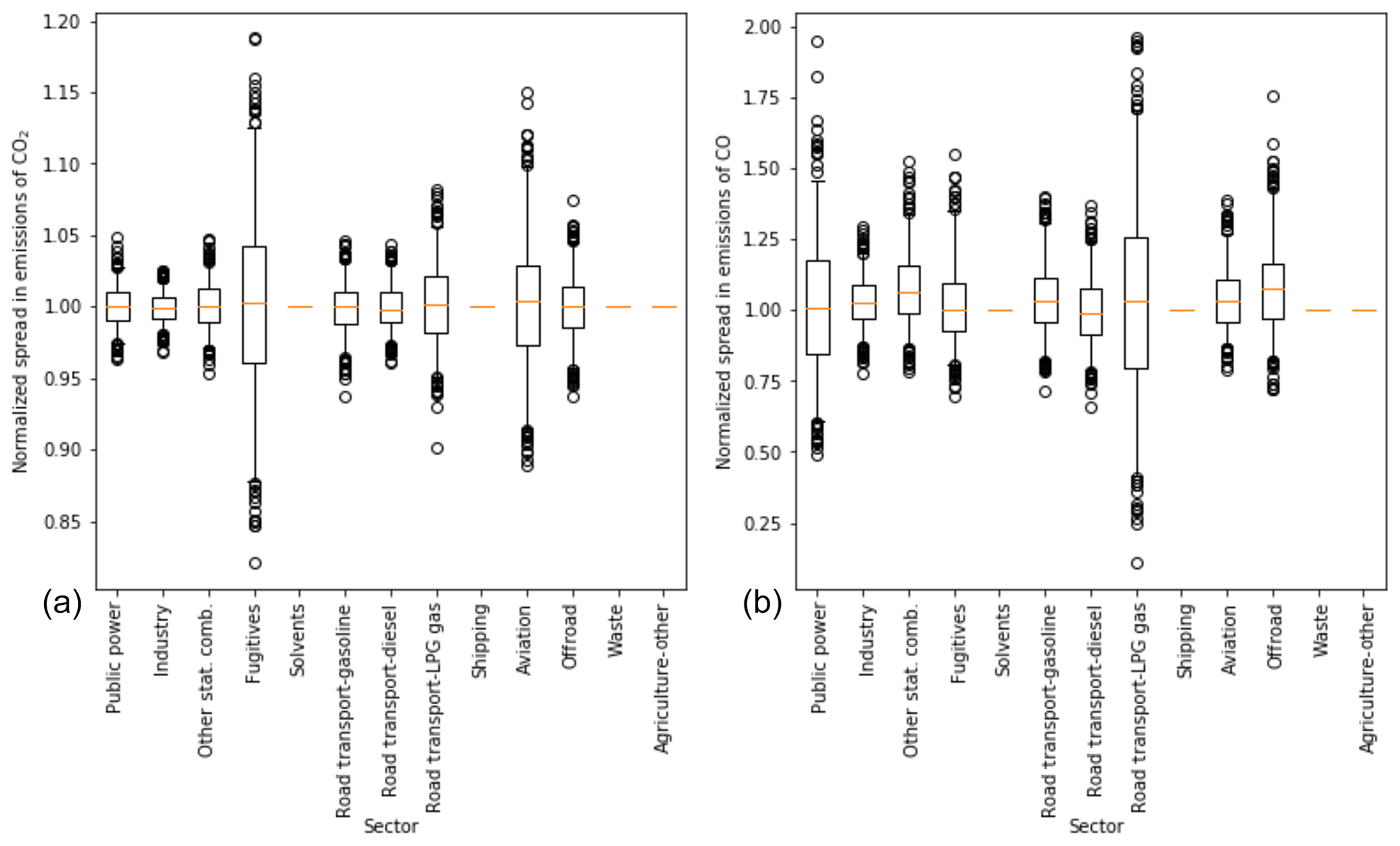
Figure 7Normalized spread in emissions of CO2 (a) and CO (b). The box represents the interquartile range, the whiskers the 2.5–97.5 percentiles, the lines the median values, and the circles are outliers. For sectors where no box is drawn, there are no data included in the Monte Carlo simulation. Note the different scales of the y axis.
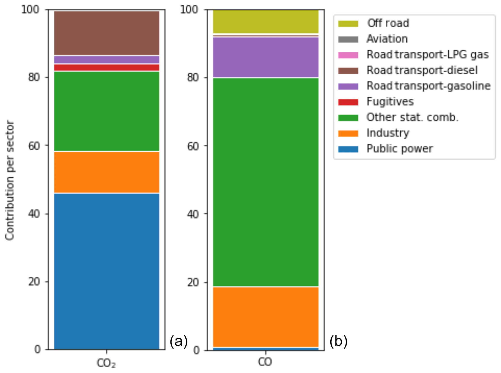
Figure 8Contribution of source sectors to the total uncertainty in CO2 (a) and CO emissions (b), summing to 100 %.
In contrast, the CO emissions show a larger uncertainty bandwidth, with many high outliers caused by the lognormal distribution of uncertainties in the emission factors. The uncertainty in the total emissions is 6 % for CO (standard deviation). Here, again, the largest uncertainties are related to sectors (public power and road transport (LPG fuel)) that are relatively small contributors to the total CO emissions. The main contributor to the uncertainty in total CO emissions is other stationary combustion, which contributes about 31 % to the total emissions and is responsible for more than 60 % of the total uncertainty.
Although the uncertainty in each parameter is assumed to be the same for each country, how a sector is composed of subsectors can vary per country. Therefore, the uncertainty per aggregated sector can also vary per country. An example is shown in Fig. 9a, which shows the normalized spread in CO2 emissions of other stationary combustion for all countries within the domain. We find a much larger uncertainty in countries where the relative fraction of biomass combustion is larger, because biomass burning has a much larger uncertainty in both the activity data and the emission factor. For example, the percentage of biomass burning in the residential sector is 54 % for the Czech Republic and 65 % for Denmark, compared to only 11 % and 9 % for the Netherlands and Great Britain. Thus, differences in the fuel composition of countries result in differences in the overall emission uncertainties, even if the uncertainty per parameter is estimated to be the same. For the total CO2 emissions, the differences between countries are small, with standard deviations between 1.2 % and 2.3 % (Fig. 9b).
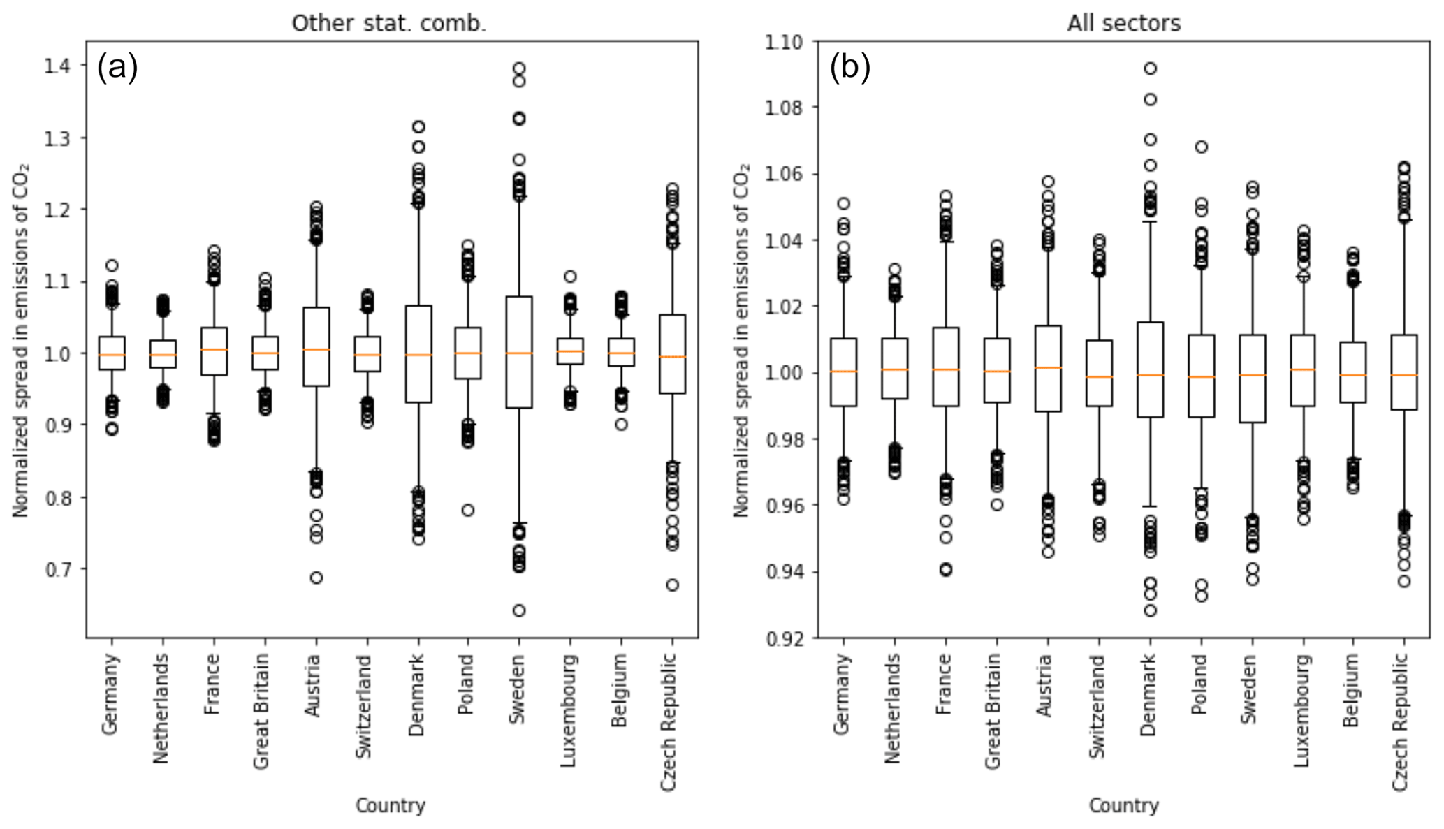
Figure 9Normalized spread in emissions of CO2 for other stationary combustion (a) and all sectors combined (b) for a range of countries. The box represents the interquartile range, the whiskers the 2.5–97.5 percentiles, the lines the median values, and the circles are outliers.
3.2 Uncertainties in spatial proxies
We examined the impact of uncertainties in spatial proxies on modelled CO2 and CO concentrations for major source sectors. For CO2, we selected other stationary combustion (only commercial/residential; no agriculture/forestry/fishing). The largest fraction (> 90 %) of CO2 emissions from this sector is distributed using population density as proxy, which is used here (the remainder of the emissions is not considered). The uncertainty in this sector–proxy combination is estimated to be 50 % (normal distribution), mainly due to the disaggregation to the 1×1 km resolution. For CO, we selected road transport (all fuels but only passenger cars). The spatial proxy for distributing passenger car emissions is based on traffic intensities compiled using Open Transport Map and Open Street Map, vehicle emission factors per road type/vehicle type/country and fleet composition. The uncertainty in this proxy is estimated to be 30 % (normal distribution) due to a higher intrinsic resolution.
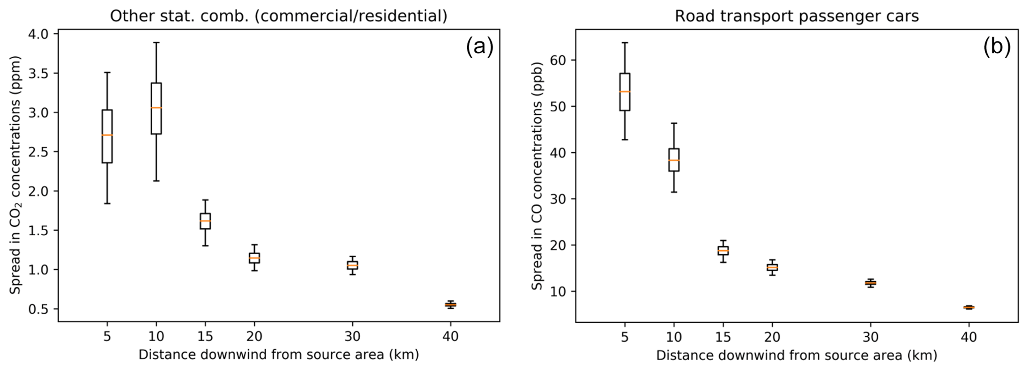
Figure 10Spread in simulated concentrations of CO2 resulting from commercial/residential emissions due to uncertainties in the total population proxy map (a) and spread in concentrations of CO resulting from road transport (passenger cars) emissions due to uncertainties in the passenger cars proxy map (b). The box represents the interquartile range, the whiskers the 2.5–97.5 percentiles, and the lines the median values of the full ensemble.
Figure 10 shows the resulting spread in atmospheric concentrations as a function of downwind distance from the source area. Note that the concentrations are enhancements caused by local emissions of the selected source sectors and do not include ambient concentrations or other sources. For CO2 (Fig. 10a), we see a concentration of about 3.0 ppm at 10 km from the source area centre but with a large uncertainty bandwidth. This signal is large enough to measure, but with this large uncertainty such measurements are difficult to use in an inversion. The measurement at 5 km from the source area centre is slightly lower than the one at 10 km, because it is upwind of a part of the emissions. At longer distances, the concentration enhancement decreases drastically and so does the absolute spread in concentrations. The enhancement becomes too small compared to the uncertainties occurring in a regular inversion framework to be useful. Figure 10b shows a similar picture for the CO concentrations resulting from passenger car emissions. Again, the spread in concentrations is large close to the source area centre and decreases with distance, but also the absolute concentration enhancement decreases. However, in this case, the concentration at 5 km from the source area centre is larger, because it is very close to an emission hotspot (see also Fig. 6). Note that we focus here on a single source sector and the overall enhancements will be larger and therefore easier to use. Nevertheless, the large spread in concentrations shows that a good representation of the spatial distribution is important for constraining sectoral emissions.
Both proxy maps discussed here are the main proxy maps for the selected sectors. As mentioned before, some sectors have residual emissions that are distributed using an alternative proxy map. An example is public power. Large power plants are listed in databases, including the reported emissions (Table 3). The remainder of the country emissions is spatially distributed over all industrial areas. However, it is more likely that the residual emissions should be attributed to specific point sources (small power plants not listed in databases). That means that instead of spreading the emissions over a large area, leading to very small local emissions and a low concentration gradient, there could be relatively large emissions at a few locations. Therefore, the uncertainty in these sector–proxy combinations is assumed to have a lognormal distribution, in part because of the absence of a better estimation.
We illustrate the effect of this assumption by creating a new proxy map for residual (small) power plants. We find that for the Netherlands a total capacity of 3655 MWe by 676 combustion plants is not included as a point source (source: S&P Global Platts World Electric Power Plants database (https://www.spglobal.com/platts/en/products-services/electric-power/world-electric-power-plants-database, last access: 25 April 2019)). At least 70 % of this capacity, attributed to 280 plants, is assumed to be in industrial areas. Given 4052 grid cells designated as industrial area in the Netherlands, this is just 7 % of the total amount of industrial area grid cells assuming no more than one plant per grid cell. The remainder is mainly related to cogeneration plants from glasshouses, which are located outside the industrial areas. Therefore, we create a new proxy map for power plants by equally assigning 70 % of the emissions from the residual power plants to 20 randomly chosen pixels (7 % of the total amount of industrial area pixels in the case study area, i.e. the same density as for the Netherlands as a whole). As mentioned before, we also raise the height of the emissions from surface level to 20 m, which is a better estimate of the stack height for small power plants.
The effect on local measurements is large (Fig. 11). Instead of measuring a small and constant signal from this sector, the assumed presence of small power plants results in measuring occasional large peak concentrations. Thus, despite being relatively unimportant at the national level, for local studies, the impact of the uncertainty in these “residual” proxies can be large.

Figure 11Spread in simulated concentrations of CO2 resulting from public power emissions due to differences in the proxy map: emissions are distributed using the new proxy map with only 20 randomly chosen pixels containing emissions. The box represents the interquartile range, the whiskers the 2.5–97.5 percentiles, the lines the median values, and the black circles are outliers of the full ensemble. The red dots show concentrations of CO2 when the original proxy map is used (industrial area).
3.3 Uncertainties in temporal profiles
The timing of emissions is important to interpret measurements correctly. During morning rush hour, a peak is expected in road traffic emissions, but the magnitude of this peak can differ from one day to the next. Also, the seasonal cycle in emissions due to heating of buildings can vary between years due to varying weather conditions. Yet, often fixed temporal profiles are used to describe the temporal disaggregation of annual emissions. The range of possible values for the temporal profile of other stationary combustion is shown in Fig. 12. The range can be very large, especially during the winter. However, note that the average of each temporal profile is 1.0 for a full year, so that the temporally distributed emissions add up to the annual total. Therefore, changes in the temporal profile indicate shifts in the timing in the emissions and not changes in the overall emissions due to cold weather, which are accounted for by the activity data.
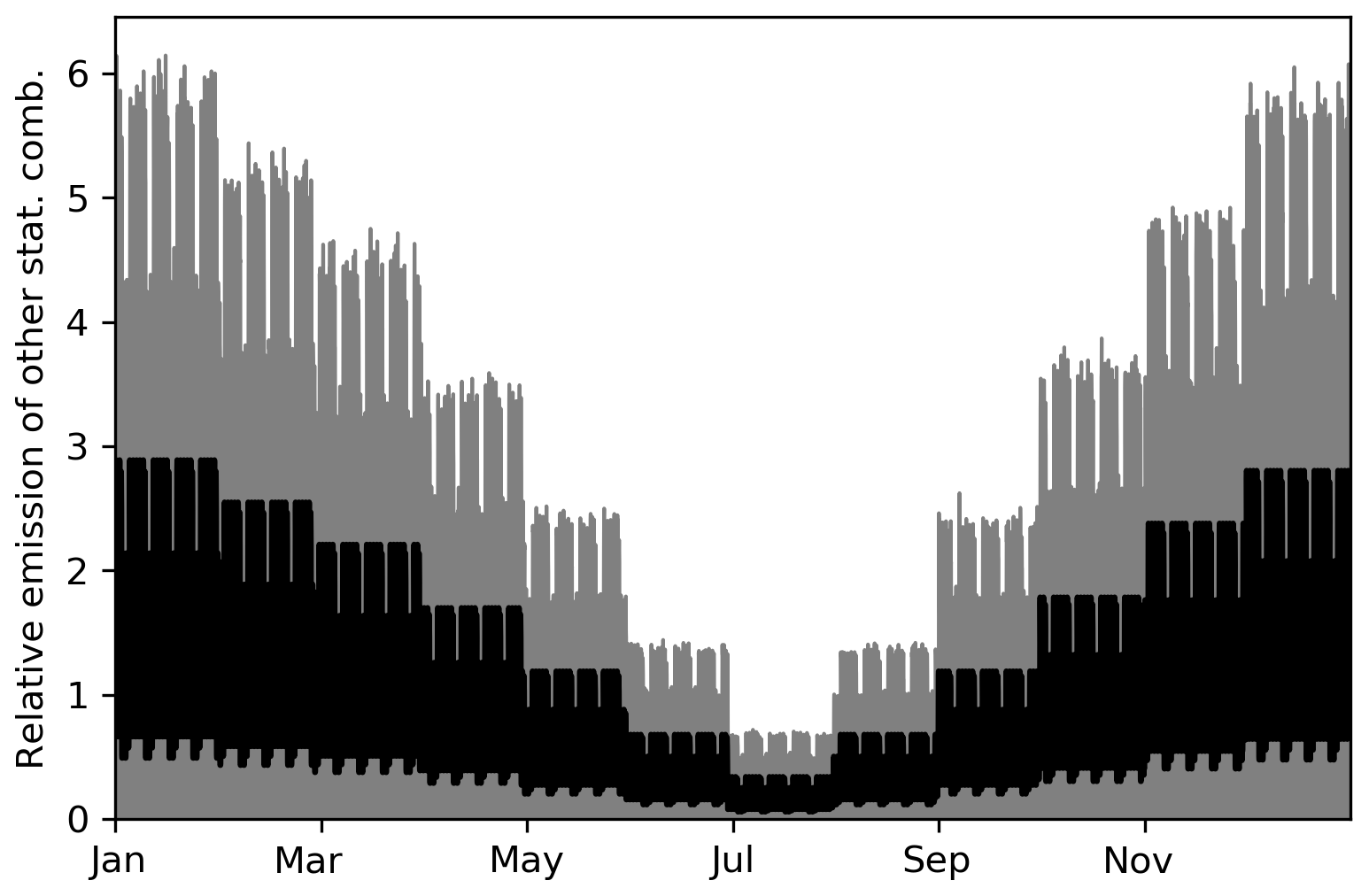
Figure 12Spread in temporal profiles for other stationary combustion (N=500), resulting from the Monte Carlo simulation (grey shading). The black line represents the standard time profile.
In inverse modelling, often well-mixed (non-stable) daytime measurements are selected (Boon et al., 2016; Breón et al., 2015; Lauvaux et al., 2013), because these are least prone to errors in model transport. For local studies, where transport times are short, this means that only afternoon emissions are optimized. The total annual emissions can then be calculated using a temporal profile. However, if the temporal profile is not correct, an incorrect fraction of the emissions can be attributed to the selected hours. We examined the impact of using an incorrect temporal profile on the total yearly emissions by calculating yearly emissions for each ensemble member. Figure 13 shows the normalized spread in sectoral emissions for all ensemble members. The error in the total annual emissions, resulting from the upscaling of daytime emissions using an incorrect temporal profile, can reach up to about 1 %–2 %. This is a significant source of error for country-level CO2 emissions but less important for CO, as the other uncertainties for CO are much larger.

Figure 13Normalized spread in emissions of CO2 and CO per sector due to uncertainties in temporal profiles. The box represents the interquartile range, the whiskers the 2.5–97.5 percentiles, the lines the median values, and the circles are outliers. The spread is the same for CO2 and CO, because they have the same temporal profiles.
3.4 Uncertainty maps and spatial patterns
As mentioned before, the uncertainty of the emission value in a grid cell is determined by the uncertainties in activity data, emission factors and spatial distribution proxies. The gridded uncertainty maps in Figs. 14 and 15 illustrate that countries or (types of) regions differ significantly in their emission uncertainty, both in absolute and relative values. Concerning the uncertainty in CO2 and CO emissions, several observations can be made.
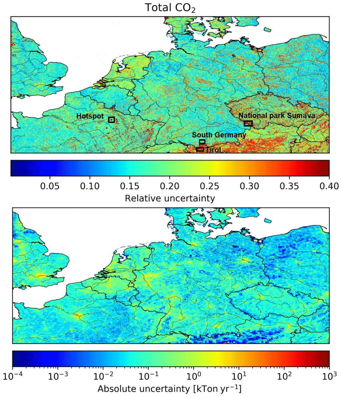
Figure 14Maps of the relative and absolute uncertainty in CO2 emissions. Areas that are examined in more detail are outlined by black squares in the top panel.
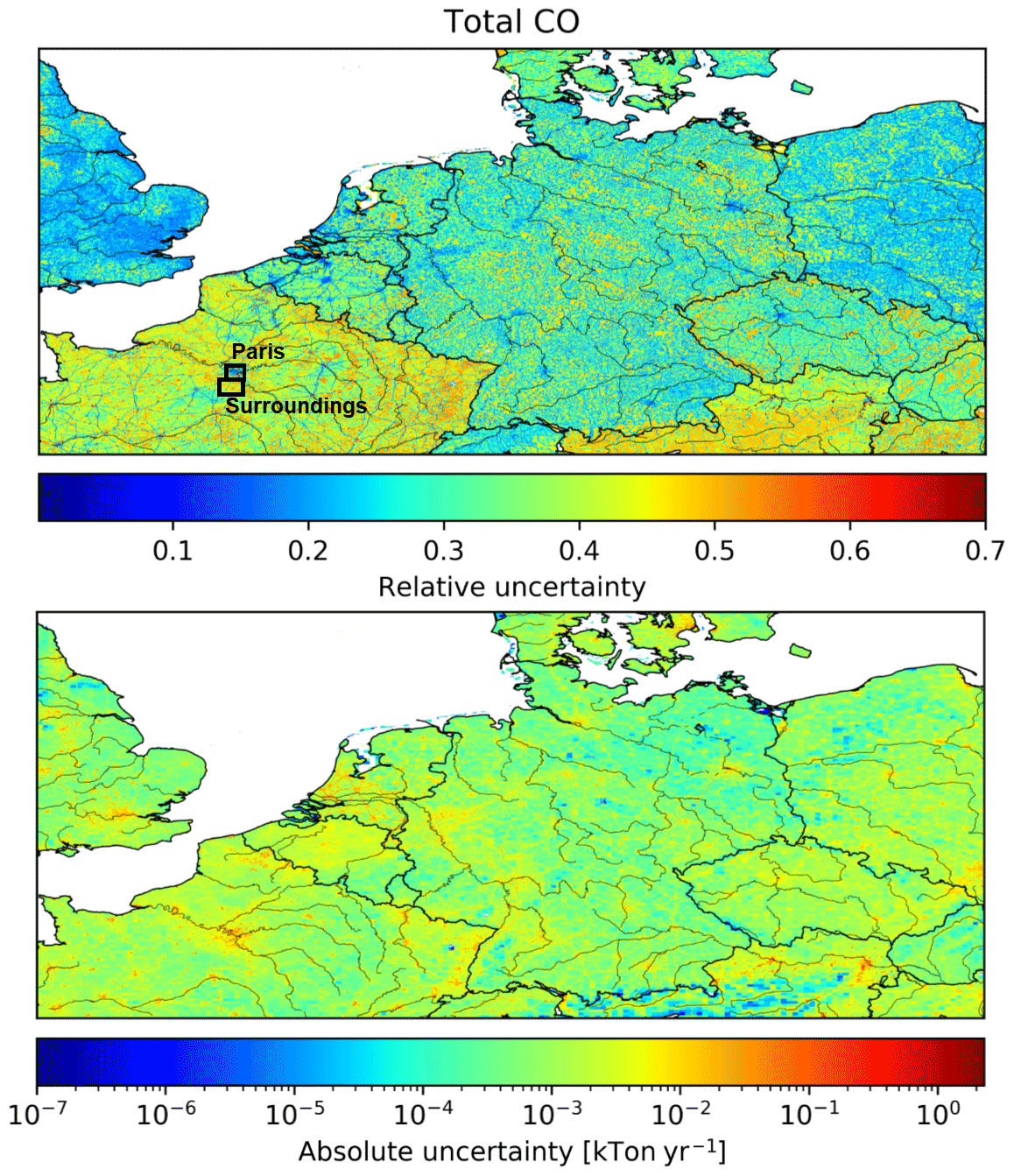
Figure 15Maps of the relative and absolute uncertainty in CO emissions. Areas that are examined in more detail are outlined by black squares in the top panel.
First, for both CO and CO2, the road network is visible due to low relative uncertainties and high absolute uncertainties compared to the surroundings. This indicates that, despite having large emissions per pixel, the spread in road traffic emissions among ensemble members is relatively small. This is likely due to the small (normally distributed) uncertainty in the spatial proxies for road traffic; i.e. the location of the roads is well known. The surrounding rural areas are dominated by other stationary combustion, which has a slightly larger spatial uncertainty.
Second, in Austria (Tirol mainly), a large area of high relative uncertainty in CO2 emissions is visible (average pixel emission is 220 t CO2 yr−1), which we compare to an area just on the other side of the border in southern Germany (average pixel emission is 495 t CO2 yr−1). The uncertainty in both areas is dominated by other stationary combustion. Yet, in Austria, a lot of biofuel is used (52 % of the total emissions for this source sector) with a large uncertainty in the emission factor and spatial distribution, whereas in Germany only 20 % of the emissions in this sector are caused by biofuel combustion. On the other hand, the absolute uncertainty is very small in Tirol because of the low population density (and thus small emissions) in this mountainous area.
Third, some large patches of high relative uncertainty in CO2 emissions are visible in the Czech Republic and the northeast of France. The location of these patches seems to correspond to natural areas/parks. Therefore, absolute uncertainties are low in these areas given the low emissions (average pixel emission in the Sumava national park is 22 t CO2 yr−1). The total uncertainty can be explained for 60 % by the uncertainty in other stationary combustion, mainly wood burning (Fig. 16). Also, agriculture (field burning of residues) plays a significant role. In addition to these natural areas, there are also some very small dark red areas (relative uncertainty) in northern France. These areas are military domain and have a lower absolute uncertainty than their surroundings because very few emissions are distributed to these areas (average pixel emission is 250 t CO2 yr−1). The public power and industrial emissions are probably too small to be reported, hence the large relatively uncertainty.
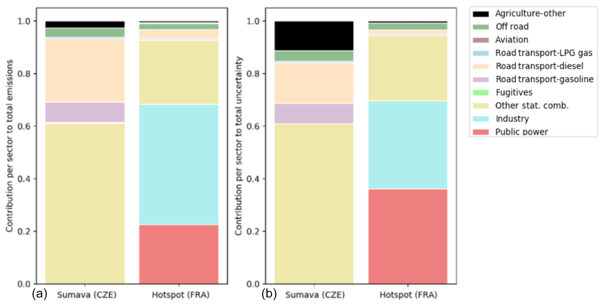
Figure 16Contribution of source sectors to the total emissions (a) and the total uncertainty (b) in CO2 for the Sumava national park in the Czech Republic and a hotspot in France, summing to 100 %. See Fig. 14 for the exact locations of these areas.
Fourth, strongly urbanized areas like Paris, the Ruhr area in Germany and Rotterdam (also see Fig. 1 for their locations) are clearly visible as areas where the relative uncertainty in CO emissions is lower than in the surrounding areas. Compared to its surroundings, the uncertainty in Paris is mainly determined by the industrial sector (Fig. 17). Since industrial emissions are relatively well known, the relative uncertainty is small. However, the absolute uncertainty is large for big cities because of the high emissions in these densely populated areas (average pixel emission is 64 t CO yr−1 for Paris). In the surrounding areas, the emissions are again dominated by other stationary combustion, which has a larger uncertainty. Yet, the absolute uncertainty is smaller because of the lower emissions (average pixel emission is 12 t CO yr−1).
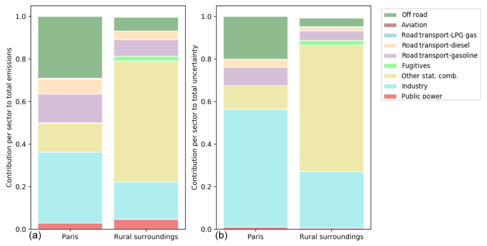
Figure 17Contribution of source sectors to the total emissions (a) and the total uncertainty (b) in CO for Paris and its surroundings, summing to 100 %. See Fig. 15 for the exact locations of these areas.
Finally, the relative uncertainties seem to be consistently higher in some countries than in others. For example, the relative uncertainty in the total emissions of France and Great Britain (only pixels within the domain) are 39 % and 25 %, respectively. For France, the main sources of uncertainty are industry and other stationary combustion, whereas the off-road and road transport sectors have a significant contribution to the uncertainty in Great Britain (Fig. 18). The main difference between the countries is again the amount of biomass used in the other stationary combustion sector (26 % in France and 8 % in Great Britain). This is likely to explain why in rural areas the relative uncertainty is much higher in France.

Figure 18Contribution of source sectors to the total emissions (a) and the total uncertainty (b) in CO for France and Great Britain, summing to 100 %.
Several previous studies have examined the uncertainty in emissions, either globally or nationally. For example, Andres et al. (2014) studied the uncertainty in the Carbon Dioxide Information Analysis Center (CDIAC) emission inventory on a global scale, suggesting that the largest uncertainties are related to the fuel consumption (i.e. activity data). A similar concern was identified for China, for which the uncertainty in energy statistics resulted in an uncertainty ratio of 15.6 % in the 2012 CO2 emissions (Hong et al., 2017). In the present study, the uncertainties in activity data and emission factors are similar for CO2, whereas the uncertainty in CO emission factors is much larger than the uncertainty in activity data. A possible explanation for this is that the energy statistics for the European countries included here are more reliable than for developing countries. The occurrence of large differences in the reliability of reported emissions between countries is also illustrated by Andres et al. (2014). In addition to these scientific studies, many countries report uncertainties in emission estimates in their National Inventory Reports (UNFCCC, 2019). Yet, their methods for uncertainty calculation differ and can even vary over time. Several scholars have examined the uncertainty in national greenhouse gas emissions in more detail. For example, Monni et al. (2004) (Finland) and Fauser et al. (2011) (Denmark) used a Tier 2 approach (Monte Carlo simulation) to determine the uncertainty in the total greenhouse gas emissions (in CO2 equivalents). They found an uncertainty of about 5 %–6 % for the year 2001 for Finland and an uncertainty of 4 %–5 % for the year 2008 for Denmark, also considering non-normal distributions in uncertainties. Moreover, Oda et al. (2019) found a 2.2 % difference in total CO2 emissions in Poland between two emission inventories, which is in agreement with our total CO2 emission uncertainty.
Even fewer studies have focused on uncertainties in the proxy maps used for spatial disaggregation. Some studies compared emission inventories to get an idea of the spatial uncertainties (Gately and Hutyra, 2017; Hutchins et al., 2017), but these studies are likely to underestimate uncertainties due to systematic errors that occur when different emission inventories use similar methods and/or proxies for spatial allocation. Moreover, exact quantification of uncertainties is often limited, dependent on the spatial scale, and the uncertainties are not specified per source (i.e. total emissions and spatial disaggregation) (Oda et al., 2019). Sowden et al. (2008) used a qualitative approach to identify the uncertainty of different components of their emission inventory for reactive pollutants (activity, emission factors, spatial and temporal allocation and speciation) by giving each component a quality rating. They suggest that spatial allocation is an important source of uncertainty for residential burning but not so much for point sources and road traffic. Indeed, the locations of large point sources and roads are relatively well known. However, we consider the allocation of emissions to pixels that include roads to have a significant (pixel value) uncertainty. Therefore, our results show that uncertainties in the spatial proxy used for road traffic can cause a significant spread in CO concentrations.
Andres et al. (2016) did a more extensive analysis of the spatial distribution in CDIAC, including uncertainties in pixel values (e.g. due to incorrect accounting methods or changes over time) and due to the representativeness of the proxy for the spatial distribution of emissions (also see Sect. 2.2.3). We considered these sources of uncertainty as well. However, Andres et al. (2016) also mention spatial discretization as a source of error, because they assign each pixel (1×1∘ resolution) to one country. The proxy maps used in this study include country fractions in each pixel, reducing this uncertainty. In contrast, we suggest another source of uncertainty, namely the fact that some pixels can include emissions while no activity takes place there, or vice versa (proxy quality). Based on the listed uncertainties, Andres et al. (2016) found an average uncertainty (2σ) in individual pixels of 120 % (assuming normal distributions). Here, we find an average uncertainty (2σ) of 36 %. However, a small number of large outliers occur (less than 0.01 % of the pixels has an uncertainty of > 1000 %) due to lognormal error distributions, although these are related to pixels with small emissions. A large part of the difference can be explained by the large pixel size of CDIAC and the large error introduced by spatial discretization (e.g. due to pixels that cover large areas of two different countries). Also, their emissions are spatially distributed based on population density, while we use a range of proxy maps depending on the source sector and use specific locations for large point sources. However, the uncertainty estimates are partially based on expert judgement and remain subjective. Moreover, the uncertainty related to the location of actual activities is not included in our uncertainty estimate, even though we have shown this can have a large impact locally.
The country-level CO2 emissions used for our emission inventory are based on NIRs, which are assumed to be relatively accurate because of the use of detailed fuel consumption statistics and country-specific emission factors (Andres et al., 2014; Francey et al., 2013). The uncertainties reported in the NIRs were determined following specified procedures and are deemed the most complete and reliable estimates available. Yet, because of the use of prescribed methods and in some cases general emission factors, systematic errors can occur both in the estimate of parameters and in the estimate of uncertainties. We choose to average the uncertainties reported by several countries, because the uncertainty estimates are relatively consistent across countries. However, this would not eliminate such systematic errors. The effect of systematic errors could be analysed by comparing different sources of information. Additionally, we assume point source emissions are relatively certain, yet a recent study showed that significant uncertainties exist in reported emissions of US power plants (Quick and Marland, 2019). A similar study for Europe is recommended, not only to improve the knowledge for the European situation but also to understand continental differences.
One source of uncertainty that is not considered in this study is the incompleteness of the emission inventory (i.e. if sources are missing) or double-counting errors. For example, during the compilation of the base inventory, we found that in several cases the CO2 emissions from airports were very low. The reason was that emissions from international flights are not reported in the NIRs and are therefore not part of the emission data used to create the inventory. Once discovered, this was corrected, and aircraft landing and take-off emissions from international flights were added in a later stage. Such discrepancies caused by reporting guidelines could be present for other source types as well. Although overall this error is likely to be small, locally the errors might be significant.
Finally, Sowden et al. (2008) mention (dis)aggregation as another source of error, i.e. the calculation of emissions on a different scale (spatially, temporally or at sector level) than the input data. In principle, fuel consumption data are available on aggregated levels and then separated over different subsectors. This increases the uncertainty at the lower level, but on the aggregated level the uncertainties remain the same. A similar note was made by Andres et al. (2016) about the use of higher-resolution proxy maps, which might increase the uncertainty due to lack of local data. However, when local data are available, this might also decrease the uncertainties. For example, the EDGAR emission database uses non-country-specific emission factors based on technology levels and sector aggregated energy statistics (Muntean et al., 2018). The reason is that the level of detail we used in this paper is not available globally. However, using generic emission factors can introduce large uncertainties when subsectoral chances occur. Therefore, regional/local studies could benefit from using a dedicated emission inventory for their region of interest instead of a global inventory.
Our results can be used to support network design and inverse modelling. The uncertainty maps are helpful to identify regions with large emission uncertainties, which can be the focus point of an inversion with the aim to optimize emissions in those regions. However, inverse modelling requires an observational network that is sensitive to the emissions from the regions of interest. A site is sensitive to specific emissions when it is often affected by them, taking into account the dominant wind direction and the magnitude of concentration enhancements, which should be larger than the uncertainties that affect model–observation comparison (e.g. measurement uncertainty and model errors). Plumes from emission hotspots can travel a long distance, and sites up to 30 km downwind have shown to be able to detect urban signals (Super et al., 2017a; Turnbull et al., 2015). The concentration enhancement in these plumes is large and therefore easy to detect. In contrast, the concentration enhancements of a single source (sector) are much smaller, as shown in Figs. 10 and 11, and therefore they become undetectable at much shorter distances. For example, vehicle exhaust emissions were shown to decrease by a factor 2 at 200 m from a highway (Canagaratna et al., 2010), while power plants plumes have been detected several kilometres downwind (Lindenmaier et al., 2014). Dilution is strongly dependent on the atmospheric conditions, and also the height of the measurement site plays an important role. To conclude, the optimal network design is strongly dependent on which question needs to be answered and the focus area and resolution needed to reach this goal.
In this work, we studied the uncertainties in a high-resolution gridded emission inventory for CO2 and CO, considering uncertainties in the underlying parameters (activity data, emission factors, spatial proxy maps and temporal profiles). We find that all factors play a significant role in determining the emission uncertainties, but that the contribution of each factor differs per sector. Disaggregation of emissions introduces additional sources of uncertainty, which makes uncertainties at a higher resolution larger than at the scale of a country/year and can have a large impact on (the interpretation of) local measurements. This is an important consideration for inverse modellers, and our methodology can be used to better define local uncertainties for, e.g. urban inversions. Inverse modellers should be aware that the use of erroneous temporal profiles to extrapolate emission data could result in errors of a few percent, which for CO2 is significant. In the future, the temporal profiles could be improved by using detailed activity data, e.g. from power plants. Moreover, we found that large regional differences exist in absolute and relative uncertainties. By looking in more detail at specific regions (or countries), more insight can be gained about the emission landscape and the main causes of uncertainty. Interestingly, areas with larger absolute uncertainties often have smaller relative uncertainties. A likely explanation is that large sources of CO2 and CO emissions received more attention and are therefore relatively well constrained, for example, in the case of large point sources. Nevertheless, since we are most interested in absolute emission reductions, the map with absolute uncertainties can be used to define an observational network that is able to reduce the largest absolute uncertainties. Finally, we believe that an uncertainty product based on a well-defined, well-documented and systematic methodology could be beneficial for the entire modelling community and support decision-making as well. However, specific needs can differ significantly between studies, for example, the scale/resolution, source sector aggregation level and which species are included. Therefore, the creation of a generic uncertainty product is challenging and needs further research.
Table A1Relative uncertainties (fraction) in activity data and CO2 emission factors as taken from the NIRs (country average) and in CO emission factors as derived from literature (assumed equal for all countries in the domain). The quoted uncertainty ranges are assumed to be representative of 1 standard deviation. Uncertainties in activity data and CO2 emission factors are often relatively low and symmetrically distributed, and normal distributions (Norm) are assumed for these activities. Compared to CO2 emission factors, the uncertainty in CO emission factors is much higher, up to an order of magnitude. Uncertainties in CO emission factors are often lognormally distributed (Logn) and are assumed equal for all countries in the HR domain. The uncertainty in the activity of open burning of waste (not covered by the NIRs) is also assumed to have a lognormal distribution.

Table A2Relative uncertainties (fractions) at cell level resulting from the spatial distribution. The values listed represent the (1 standard deviation) uncertainty of the emission per cell due to uncertainty sources 2 and 3 as listed in Sect. 2.2.3. All values in the table below are based on expert quantification and inevitably include a considerable amount of subjectivity. The data should therefore be considered as a first-order indication only. Note that the natural logarithm (Ln) of the uncertainty fraction is given in the event that uncertainty has a lognormal distribution.
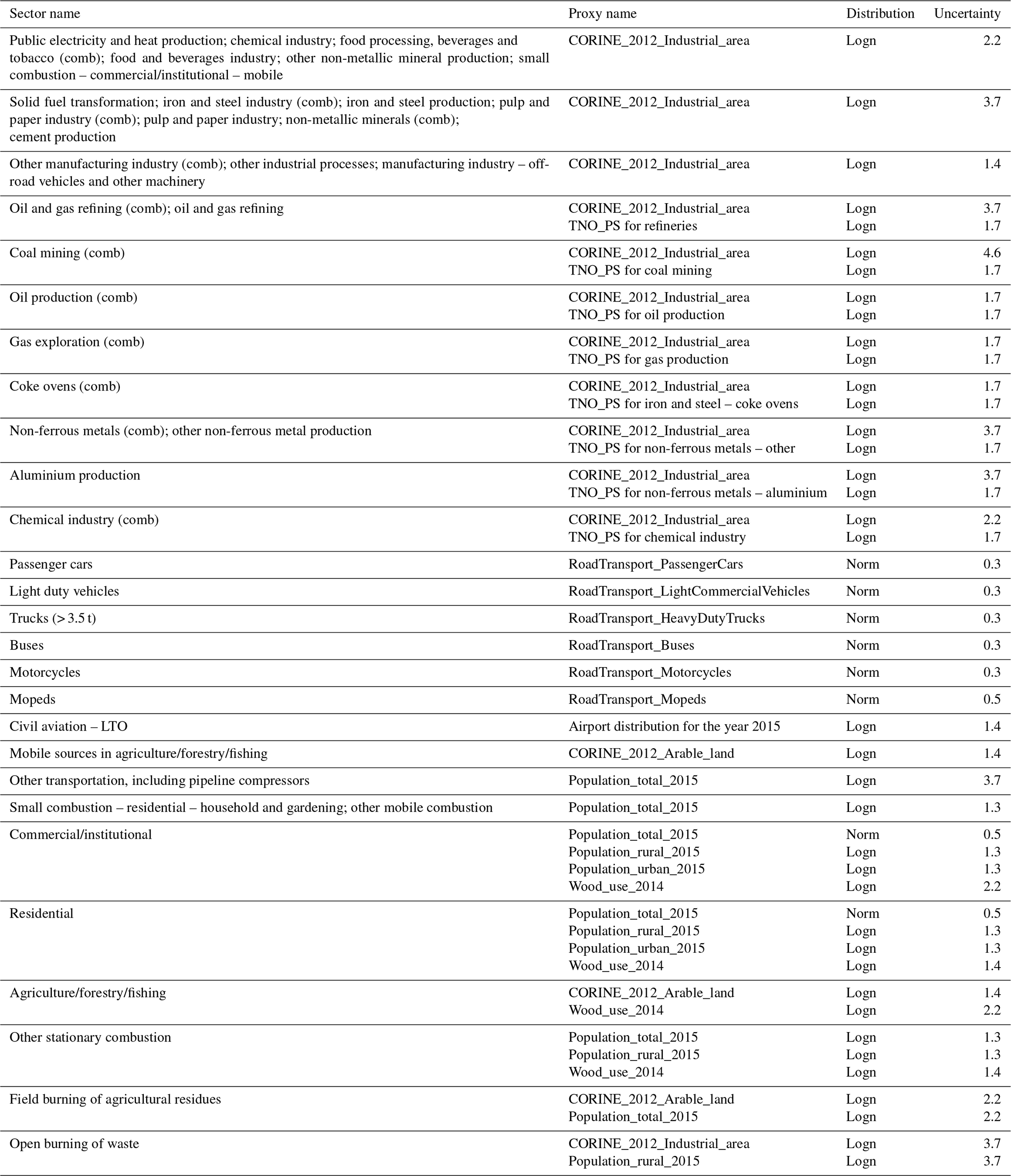
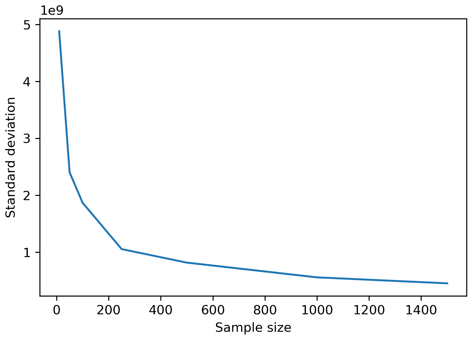
Figure B1Spread in the standard deviations if the Monte Carlo simulation were to be repeated multiple times for a specific sample size, based on a bootstrapping method.
The family of 10 emission inventories is available for non-commercial applications and research (https://doi.org/10.5281/zenodo.3584549, Super et al., 2019).
AJHV assembled the uncertainty data used in this work. SNCD and HACDvdG are responsible for the base emission inventory. IS designed the experiments, carried them out and prepared the manuscript with contributions from all co-authors.
The authors declare that they have no conflict of interest.
This study was supported by the CO2 Human Emissions (CHE) project, funded by the European Union's Horizon 2020 research and innovation programme under grant agreement no. 776186 and the VERIFY project, funded by the European Union's Horizon 2020 research and innovation programme under grant agreement no. 776810.
This research has been supported by the European Commission (project CHE (grant no. 776186) and project VERIFY (grant no. 776810)).
This paper was edited by Ronald Cohen and reviewed by two anonymous referees.
Amann, M., Bertok, I., Borken-Kleefeld, J., Cofala, J., Heyes, C., Höglund-Isaksson, L., Klimont, Z., Nguyen, B., Posch, M., Rafaj, P., Sandler, R., Schöpp, W., Wagner, F., and Winiwarter, W.: Cost-effective control of air quality and greenhouse gases in Europe: Modeling and policy applications, Environ. Modell. Softw., 26, 1489–1501, https://doi.org/10.1016/j.envsoft.2011.07.012, 2011.
Andres, R. J., Boden, T. A., and Higdon, D.: A new evaluation of the uncertainty associated with CDIAC estimates of fossil fuel carbon dioxide emission, Tellus B, 66, 1–15, https://doi.org/10.3402/tellusb.v66.23616, 2014.
Andres, R. J., Boden, T. A., and Higdon, D. M.: Gridded uncertainty in fossil fuel carbon dioxide emission maps, a CDIAC example, Atmos. Chem. Phys., 16, 14979–14995, https://doi.org/10.5194/acp-16-14979-2016, 2016.
Berner, R. A.: The long-term carbon cycle, fossil fuels and atmospheric composition, Nature, 426, 323–326, https://doi.org/10.1038/nature02131, 2003.
Boon, A., Broquet, G., Clifford, D. J., Chevallier, F., Butterfield, D. M., Pison, I., Ramonet, M., Paris, J. D., and Ciais, P.: Analysis of the potential of near-ground measurements of CO2 and CH4 in London, UK, for the monitoring of city-scale emissions using an atmospheric transport model, Atmos. Chem. Phys., 16, 6735–6756, https://doi.org/10.5194/acp-16-6735-2016, 2016.
Boschetti, F., Thouret, V., Maenhout, G. J., Totsche, K. U., Marshall, J., and Gerbig, C.: Multi-species inversion and IAGOS airborne data for a better constraint of continental-scale fluxes, Atmos. Chem. Phys., 18, 9225–9241, https://doi.org/10.5194/acp-18-9225-2018, 2018.
Breón, F. M., Broquet, G., Puygrenier, V., Chevallier, F., Xueref-Remy, I., Ramonet, M., Dieudonné, E., Lopez, M., Schmidt, M., Perrussel, O., and Ciais, P.: An attempt at estimating Paris area CO2 emissions from atmospheric concentration measurements, Atmos. Chem. Phys., 15, 1707–1724, https://doi.org/10.5194/acp-15-1707-2015, 2015.
Canagaratna, M. R., Onasch, B. T., Wood, E. C., Herndon, S. C., Jayne, J. T., Cross, E. S., Miake-Lye, R. C., Kolb, C. E., and Worsno, D. R.: Evolution of vehicle exhaust particles in the atmosphere, J. Air Waste Manag., 60, 1192–1203, https://doi.org/10.3155/1047-3289.60.10.1192, 2010.
Denier van der Gon, H. A. C., Hendriks, C., Kuenen, J., Segers, A., and Visschedijk, A.: Description of current temporal emission patterns and sensitivity of predicted AQ for temporal emission patterns, TNO, Utrecht, the Netherlands, 1–22, 2011.
Denier van der Gon, H. A. C., Kuenen, J. J. P., Janssens-Maenhout, G., Döring, U., Jonkers, S., and Visschedijk, A.: TNO_CAMS high resolution European emission inventory 2000–2014 for anthropogenic CO2 and future years following two different pathways, Earth Syst. Sci. Data Discuss., https://doi.org/10.5194/essd-2017-124, in review, 2017.
European Environment Agency: EMEP/EEA air pollutant emission inventory guidebook 2016: Technical guidance to prepare national emission inventories, Luxembourg, 1–28, 2016.
Fauser, P., SØrensen, P. B., Nielsen, M., Winther, M., Plejdrup, M. S., Hoffmann, L., GyldenkÆrne, S., Mikkelsen, H. M., Albrektsen, R., Lyck, E., Thomsen, M., Hjelgaard, K., and Nielsen, O.-K.: Monte Carlo Tier 2 uncertainty analysis of Danish Greenhouse gas emission inventory, Greenh. Gas Meas. Manag., 1, 145–160, https://doi.org/10.1080/20430779.2011.621949, 2011.
Francey, R. J., Trudinger, C. M., Van der Schoot, M., Law, R. M., Krummel, P. B., Langenfelds, R. L., Paul Steele, L., Allison, C. E., Stavert, A. R., Andres, R. J., and Rödenbeck, C.: Atmospheric verification of anthropogenic CO2 emission trends, Nat. Clim. Change, 3, 520–524, https://doi.org/10.1038/nclimate1817, 2013.
Gately, C. K. and Hutyra, L. R.: Large uncertainties in urban-scale carbon emissions, J. Geophys. Res.-Atmos., 122, 242–260, https://doi.org/10.1002/2017JD027359, 2017.
Gurney, K. R., Zhou, Y., Mendoza, D., Chandrasekaran, V., Geethakumar, S., Razlivanov, I., Song, Y., and Godbole, A.: Vulcan and Hestia: High resolution quantification of fossil fuel CO2 emissions, in: MODSIM 2011 – 19th International Congress on Modelling and Simulation – Sustaining Our Future: Understanding and Living with Uncertainty, Perth, Australia, 12–16 December 2011, 1781–1787, 2011.
Gurney, K. R., Patarasuk, R., Liang, J., Song, Y., O'Keeffe, D., Rao, P., Whetstone, J. R., Duren, R. M., Eldering, A., and Miller, C.: The Hestia fossil fuel CO2 emissions data product for the Los Angeles megacity (Hestia-LA), Earth Syst. Sci. Data, 11, 1309–1335, https://doi.org/10.5194/essd-11-1309-2019, 2019.
Hong, C., Zhang, Q., He, K., Guan, D., Li, M., Liu, F., and Zheng, B.: Variations of China's emission estimates: Response to uncertainties in energy statistics, Atmos. Chem. Phys., 17, 1227–1239, https://doi.org/10.5194/acp-17-1227-2017, 2017.
Hutchins, M. G., Colby, J. D., Marland, G., and Marland, E.: A comparison of five high-resolution spatially-explicit, fossil-fuel, carbon dioxide emission inventories for the United States, Mitig. Adapt. Strat. Gl., 22, 947–972, https://doi.org/10.1007/s11027-016-9709-9, 2017.
IEA: World Energy Outlook 2008, Paris, 1–569, 2008.
Janssen, H.: Monte-Carlo based uncertainty analysis: Sampling efficiency and sampling convergence, Reliab. Eng. Syst. Safe, 109, 123–132, https://doi.org/10.1016/j.ress.2012.08.003, 2013.
Kuenen, J. J. P., Visschedijk, A. J. H., Jozwicka, M., and Denier van der Gon, H. A. C.: TNO-MACC-II emission inventory; A multi-year (2003–2009) consistent high-resolution European emission inventory for air quality modelling, Atmos. Chem. Phys., 14, 10963–10976, https://doi.org/10.5194/acp-14-10963-2014, 2014.
Lauvaux, T., Miles, N. L., Richardson, S. J., Deng, A., Stauffer, D. R., Davis, K. J., Jacobson, G., Rella, C., Calonder, G. P., and Decola, P. L.: Urban emissions of CO2 from Davos, Switzerland: The first real-time monitoring system using an atmospheric inversion technique, J. Appl. Meteorol. Climatol., 52, 2654–2668, https://doi.org/10.1175/JAMC-D-13-038.1, 2013.
Lindenmaier, R., Dubey, M. K., Henderson, B. G., Butterfield, Z. T., Herman, J. R., Rahn, T., and Lee, S.-H.: Multiscale observations of CO2, 13CO2, and pollutants at Four Corners for emission verification and attribution, P. Natl. Acad. Sci. USA, 111, 8386–8391, https://doi.org/10.1073/pnas.1321883111, 2014.
Monni, S., Syri, S., and Savolainen, I.: Uncertainties in the Finnish greenhouse gas emission inventory, Environ. Sci. Policy, 7, 87–98, https://doi.org/10.1016/j.envsci.2004.01.002, 2004.
Muntean, M., Vignati, E., Crippa, M., Solazzo, E., Schaaf, E., Guizzardi, D., and Olivier, J. G. J.: Fossil CO2 emissions of all world countries – 2018 report, European Commission, Luxembourg, 1–241, 2018.
Oda, T., Bun, R., Kinakh, V., Topylko, P., Halushchak, M., Marland, G., Lauvaux, T., Jonas, M., Maksyutov, S., Nahorski, Z., Lesiv, M., Danylo, O., and Joanna, H.-P.: Errors and uncertainties in a gridded carbon dioxide emissions inventory, Mitig. Adapt. Strateg. Glob. Change, 24, 1007–1050, https://doi.org/10.1007/s11027-019-09877-2, 2019.
Palmer, P. I., O'Doherty, S., Allen, G., Bower, K., Bösch, H., Chipperfield, M. P., Connors, S., Dhomse, S., Feng, L., Finch, D. P., Gallagher, M. W., Gloor, E., Gonzi, S., Harris, N. R. P., Helfter, C., Humpage, N., Kerridge, B., Knappett, D., Jones, R. L., Le Breton, M., Lunt, M. F., Manning, A. J., Matthiesen, S., Muller, J. B. A., Mullinger, N., Nemitz, E., O'Shea, S., Parker, R. J., Percival, C. J., Pitt, J., Riddick, S. N., Rigby, M., Sembhi, H., Siddans, R., Skelton, R. L., Smith, P., Sonderfeld, H., Stanley, K., Stavert, A. R., Wenger, A., White, E., Wilson, C., and Young, D.: A measurement-based verification framework for UK greenhouse gas emissions: an overview of the Greenhouse gAs Uk and Global Emissions (GAUGE) project, Atmos. Chem. Phys., 18, 11753–11777, https://doi.org/10.5194/acp-18-11753-2018, 2018.
Quick, J. C. and Marland, E.: Systematic error and uncertain carbon dioxide emissions from USA power plants, J. Air Waste Manag., 69, 646–658, https://doi.org/10.1080/10962247.2019.1578702, 2019.
Sauter, F., Van Zanten, M., Van der Swaluw, E., Aben, J., De Leeuw, F., and Van Jaarsveld, H.: The OPS-model. Description of OPS 4.5.0, RIVM, Bilthoven, 1–113, 2016.
Sowden, M., Cairncross, E., Wilson, G., Zunckel, M., Kirillova, E., Reddy, V., and Hietkamp, S.: Developing a spatially and temporally resolved emission inventory for photochemical modeling in the City of Cape Town and assessing its uncertainty, Atmos. Environ., 42, 7155–7164, https://doi.org/10.1016/j.atmosenv.2008.05.048, 2008.
Super, I., Denier van der Gon, H. A. C., Van der Molen, M. K., Sterk, H. A. M., Hensen, A., and Peters, W.: A multi-model approach to monitor emissions of CO2 and CO from an urban-industrial complex, Atmos. Chem. Phys., 17, 13297–13316, https://doi.org/10.5194/acp-17-13297-2017, 2017a.
Super, I., Denier van der Gon, H. A. C., Visschedijk, A. J. H., Moerman, M. M., Chen, H., van der Molen, M. K., and Peters, W.: Interpreting continuous in-situ observations of carbon dioxide and carbon monoxide in the urban port area of Rotterdam, Atmos. Pollut. Res., 8, 174–187, https://doi.org/10.1016/j.apr.2016.08.008, 2017b.
Super, I., Dellaert, S. N. C., Visschedijk, A. J. H., and Denier van der Gon, H. A. C.: Set of European CO2 and CO emission grids representing emission uncertainties, https://doi.org/10.5281/zenodo.3584549, 2019.
Turnbull, J. C., Sweeney, C., Karion, A., Newberger, T., Lehman, S. J., Tans, P. P., Davis, K. J., Lauvaux, T., Miles, N. L., Richardson, S. J., Cambaliza, M. O., Shepson, P. B., Gurney, K., Patarasuk, R., and Razlivanov, I.: Toward quantification and source sector identification of fossil fuel CO2 emissions from an urban area: Results from the INFLUX experiment, J. Geophys. Res.-Atmos., 120, 292–312, https://doi.org/10.1002/2013JD020225, 2015.
UNFCCC: National Inventory Submissions 2019, available at: https://unfccc.int/process-and-meetings/, last access: 24 January 2019.
Van Jaarsveld, J. A.: The Operational Priority Substances model. Description and validation of OPS-Pro 4.1, RIVM Bilthoven, the Netherlands, 1–156, 2004.
Zheng, B., Chevallier, F., Yin, Y., Ciais, P., Fortems-Cheiney, A., Deeter, M. N., Parker, R. J., Wang, Y., Worden, H. M., and Zhao, Y.: Global atmospheric carbon monoxide budget 2000–2017 inferred from multi-species atmospheric inversions, Earth Syst. Sci. Data, 11, 1411–1436, https://doi.org/10.5194/essd-11-1411-2019, 2019.