What can we learn about urban air quality with regard to the first outbreak of the COVID-19 pandemic? A case study from central Europe

Motor vehicle road traffic in central Budapest was reduced by approximately 50 % of its ordinary level for several weeks as a consequence of various limitation measures introduced to mitigate the first outbreak of the COVID-19 pandemic in 2020. The situation was utilised to assess the real potentials of urban traffic on air quality. Concentrations of NO, NO₂, CO, O₃, SO₂ and particulate matter (PM) mass, which are ordinarily monitored in cities for air quality considerations, aerosol particle number size distributions, which are not rarely measured continuously on longer runs for research purposes, and meteorological properties usually available were collected and jointly evaluated in different pandemic phases. The largest changes occurred over the severest limitations (partial lockdown in the Restriction phase from 28 March to 17 May 2020). Concentrations of NO, NO₂, CO, total particle number (N_6–1000) and particles with a diameter < 100 nm declined by 68 %, 46 %, 27 %, 24 % and 28 %, respectively, in 2020 with respect to the average reference year comprising 2017–2019. Their quantification was based on both relative difference and standardised anomaly. The change rates expressed as relative concentration difference due to relative reduction in traffic intensity for NO, NO₂, N_6–1000 and CO were 0.63, 0.57, 0.40 and 0.22 (%/%), respectively. Of the pollutants which reacted in a sensitive manner to the change in vehicle circulation, it is the NO₂ that shows the most frequent exceedance of the health limits. Intentional tranquillising of the vehicle flow has considerable potential for improving the air quality. At the same time, the concentration levels of PM₁₀ mass, which is the most critical pollutant in many European cities including Budapest, did not seem to be largely affected by vehicles. Concentrations of O₃ concurrently showed an increasing tendency with lower traffic, which was explained by its complex reaction mechanism. Modelling calculations indicated that spatial gradients of NO and NO₂ within the city became further enhanced by reduced vehicle flow.

1 Introduction

The coronavirus disease (COVID-19) is caused by the novel, Severe Acute Respiratory Syndrome CoronaVirus 2 (SARS-CoV-2) virus. The outbreak was declared a pandemic by the WHO on 11 March 2020 (WHO, 2020). National governments and international agencies and organisations enacted widespread emergency actions for individuals, some professionals, communities and the public to reduce the risk of infection and to combat the plague. As a consequence of the implemented measures, road traffic in many cities worldwide was reduced in a substantial manner and for a considerable time interval. In parallel, lower concentrations of several air pollutants were reported from both satellite observations and in situ measurements (Conticini et al., 2020; Frontera et al., 2020; Keller et al., 2020; Lal et al., 2020; Le et al., 2020; Lee et al., 2020; Liu et al., 2020; Mahato et al., 2020; Morawska and Cao, 2020; Nakada and Urban, 2020; Petetin et al., 2020; Tobías et al., 2020; Wang et al., 2020).

This situation offers a unique possibility for atmospheric scientists to investigate experimentally some important atmospheric chemical and physical issues, including urban air quality and climate change under extraordinary conditions of lower traffic and industrial productivity (Sussmann and Rettinger, 2020). The results and consequences of this real “ambient experiment” can be utilised to determine the true potentials of action plans on tranquillising urban road circulation for handling air quality, overcrowding, traffic congestions, noise contamination and other environmental, health and climate impacts in large cities.

The task is, however, somewhat complicated. Actual concentrations of atmospheric constituents can depend on (1) their emissions from several sectors, (2) their physical removal processes, (3) local meteorological conditions, mainly precipitation (P), wind speed (WS), planetary boundary layer height (PBLH) and atmospheric stability, (4) their (long-range) transport and (5) possible photochemical reactions, which are largely influenced by other meteorological properties such as global solar radiation (GRad), relative humidity (RH) and air temperature (T) and by availability of and interactions with other chemical species present in the air. Many of the phenomena or properties listed are, in addition, interconnected and confounding, which further obscures the situation since they create an internally interacting environmental system.

Tropospheric residence time of constituents can also play a role under non-steady-state conditions (Harrison, 2018). As a result, atmospheric concentrations at a fixed site change both periodically and randomly (fluctuate) on daily, seasonal or annual scales. The variations are also linked to the geographical location and features of urban sites (de Jesus et al., 2019).

Source-specific markers generated by internal combustion engines or added on purpose into their fuel (e.g. Horvath et al., 1988; Gentner et al., 2017) or multivariate statistical methods (Hopke, 2016) can be applied to estimate the importance of vehicle traffic for air quality. These methods usually require advanced analytical methods to obtain data for specific species, which may not be available with a required time resolution or need a larger number of data, which can be constrained by duration of the time intervals of interest. Another possibility is to examine jointly the time series of multicomponent atmospheric data sets. This approach (described later in more detail) can be utilised retrospectively and is generally applicable in different cities in the world, which were affected by road traffic restrictions.

In Hungary, a state of emergency was introduced on 11 March 2020. It involved sequential closure of education institutes, the beginning of working from home and social distancing. It was followed by restrictions on movement. During this, residences could only be left with specified basic purposes, administrative centres, restaurants and touristic places were closed, distant travels were ceased, public parks were closed for long weekends and there were various time limitations on shopping. The mitigating measures resulted in perceivable changes in vehicular road traffic and atmospheric concentrations. The main objectives of the present paper are (1) to introduce and demonstrate a general method for quantifying concentration changes, (2) to evaluate whether the changes observed were related to motor vehicle road traffic, (3) to assess the effect of traffic on these alterations, and (4) to estimate and debate the potentials of tranquillised urban vehicle flow for the air quality.

2 Methods

Criteria air pollutants, namely NO, NO₂ = NO_x − NO, CO, O₃, SO₂ and particulate matter (PM) mass in various size fractions, were involved in the study. The species originate from different sources. Vehicular road traffic is usually associated with NO and CO, while NO₂ and O₃ are formed by chemical reactions in the air. Contributions of residential heating, cooking, industrial activities, regional traffic in winter and secondary processes to PM_2.5 mass are of large importance in many cities, including Budapest. At the same time, PM₁₀ mass represents disintegration sources, e.g. windblown soil, crustal rock, mineral and roadside dust, resuspended dust by car movement, agricultural activities in the region, construction work and material wear such as tire abrasion of cars at kerbside sites (Salma and Maenhaut, 2006; Putaud et al., 2010; Harrison et al., 2012; Salma et al., 2020a). They all can be important, particularly under dry weather conditions.

Aerosol particle number concentrations in the diameter ranges from 6 to 1000 nm (N_6–1000) and from 6 to 100 nm (N_6–100) are mainly assigned to high-temperature emission sources (such as vehicle road traffic or incomplete burning) and atmospheric new particle formation and growth (NPF) events (Paasonen et al., 2016; Rönkkö et al., 2017; Salma et al., 2017). The latter process occurs as a daily phenomenon with a typical shape of its monthly occurrence frequency (Salma and Németh, 2019). This distribution changes in Budapest from year to year without any tendentious character (Salma et al., 2020b). Particles with a diameter from 25 to 100 nm (N_25–100) in cities are mainly emitted by incomplete combustion or consist of grown new particles by condensation, while the size fraction with a diameter from 100 to 1000 nm (N_100–1000) expresses physically and chemically aged particles; thus, they represent larger spatial extents (Salma et al., 2014; Mikkonen et al., 2020).

Approximate tropospheric residence times of NO_x, CO, O₃, SO₂ and PM are estimated to 1–2 d, 2 months, 1–2 months, 4–12 d and from several hours up to 1 week depending largely on particle size and chemical composition, respectively (Warneck and Williams, 2012; Harrison, 2018).

2.1 Experimental data

The concentrations of NO ∕ NO_x, CO, O₃, SO₂, PM₁₀ mass and PM_2.5 mass were measured by chemiluminescence (Thermo 42C), IR absorption (Thermo 48i), UV fluorescence (Ysselbach 43C), UV absorption (Ysselbach 49C) and beta-ray attenuation (two Environment MP101M instruments with PM₁₀ and PM_2.5 inlets) methods, respectively, with a time resolution of 1 h. The concentrations of gases were expressed at a temperature of 293 K and a pressure of 101.3 kPa. The particle number concentrations were determined by a flow-switching type differential mobility particle sizer (DMPS; Salma et al., 2016b) with a time resolution of 8 min. The latter measurements were performed in a diameter range from 6 to 1000 nm in 30 size channels with equal width in the dry state of particles. The meteorological data of T, RH and WS and of GRad were measured by standardised sensors (HD52.3D17, Delta OHM, Italy, and SMP3 pyranometer, Kipp and Zonen, the Netherlands, respectively) with a time resolution of 1 min.

The DMPS and meteorological measurements were accomplished at the Budapest platform for Aerosol Research and Training (BpART) Laboratory (47^∘28^′29.9^′′ N, 19^∘3^′44.6^′′ E; 115 m above mean sea level) of the Eötvös University (Fig. 1). The location represents a well-mixed, average atmospheric environment for the city centre due to its geographical and meteorological conditions (Salma et al., 2016a). The local emissions include diffuse urban traffic exhaust, household/residential emissions and limited industrial sources together with some off-road transport (Salma et al., 2020a). In some time intervals, long-range transport of air masses can also play a role.

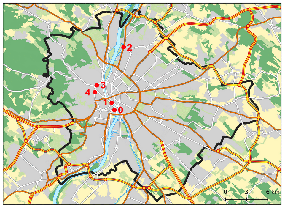
Figure 1 Location of the measurement sites in Budapest. 0: BpART Laboratory, 1: Szabadság Bridge, 2: Váci Road, 3: Széna Square and 4: Alkotás Road. The border of the city (in black colour), the Danube River and the major routes are also indicated.

The data of the criteria air pollutants were acquired from a measurement station of the National Air Quality Network at Széna Square (Fig. 1) located 4.5 km from the BpART Laboratory in the upwind-prevailing direction (Salma and Németh, 2019). This station serves as a reference for our long-term air-quality-related research activities in several aspects and proved to be acceptable for this purpose.

Atmospheric transport of chemical species was assessed through large-scale weather types. We utilised macrocirculation patterns (MCPs), which were invented specifically for the Carpathian Basin (Péczely, 1957; Maheras et al., 2018). The classification of the MCPs is based on the position, extension and development of cyclones and anticyclones relative to the Carpathian Basin considering the sea-level pressure maps constructed for 00:00 UTC in the North Atlantic–European region on a daily basis. A brief survey on the MCPs and the actual codes for year 2020 utilised in the interpretations are given in Table S1 and Fig. S1, respectively, in the Supplement. The relative occurrences of the weather types in year 2020 were roughly in line with multiple-year frequencies. Extended anticyclonic weather types usually indicate that the air masses are stagnant and that the importance of local or regional sources prevails over the air transport from distant sources. Under cyclonic weather conditions and frontal systems, the transported air masses can yield more pronounced effects and contributions.

A census of motor road vehicles was performed on three major routes and on a bridge over the Danube River by Budapest Public Roads Ltd. The measurement sites were on Szabadság Bridge, Váci Road, around Széna Square and Alkotás Road (Fig. 1), which are described in more detail in the Supplement. The counting was based on permanent electronic devices with inductive loops, and passenger cars, high- and heavy-duty vehicles and buses were recorded in both directions. The time resolution of the data was 1 h and their coverage was >90 % of all possible items in a year. The sites cover a wide range of maximum hourly mean vehicle flow from about 1200 to 4600 h⁻¹. Szabadság Bridge has the smallest traffic intensity of the sites, but it proved to be a very valuable microenvironment for the study since it is part of the internal boulevard. The routes showed coherent and common aggregate time properties and, therefore, their data are to be proportional to general vehicular traffic flow in the city centre.

2.2 Time intervals of interest

Time intervals from 1 January to 31 July in 2017, 2018, 2019 and 2020 were studied. This included all major measures related to the first outbreak of the COVID-19 pandemic in Budapest in 2020. Within these 7 months, five consecutive time intervals were selected for comparative purposes: (1) from 1 January till the beginning of the state of emergency at 15:00 on 11 March, which is referred to as the Pre-emergency phase, (2) from the beginning of the state of emergency to 27 March (till the beginning of the restriction on movement), which is called here the Pre-restriction phase, (3) from the beginning of the restriction on movement till its end in Budapest on 17 May, which is denoted the Restriction phase, (4) from the end of the restriction on movement in Budapest till the end of the state of emergency on 17 June, which is referred to as the Post-restriction phase, and (5) from the end of the state of emergency till 31 July, which is called the Post-emergency phase. An overview of the pandemic phases with further details of possible relevance for air quality issues is summarised in Fig. S1. Equivalent time intervals in year 2017–2019, which correspond to these phases, were considered for comparative purposes.

Local daylight saving time (LDST = UTC+1 or UTC+2) was chosen as the time base for the atmospheric concentrations and road traffic data because it was observed that the daily activity time patterns of inhabitants largely influence these variables in cities (Salma et al., 2014). The meteorological data were expressed in UTC+1 since their diurnal and seasonal behaviours are primarily controlled by Sun path and other natural processes.

2.3 Data treatment and modelling

Medical studies with the influenza virus indicated that absolute humidity (AH) constrains both transmission efficiency and virus survival more than RH (Shaman and Kohn, 2009). In order to facilitate the future comparison with other locations or cities in the world mainly for possible virology purposes, the hourly mean RH values (%) were converted to AH (g m⁻³) using a calculation recommended by WMO (2008):

$$\begin{array}{}\text{(1)}& \mathrm{AH}={\displaystyle \frac{e\left(T_{\mathrm{0}}\right)\times \exp \left(A\times \frac{T}{T+B}\right)\times \mathrm{RH}\times C}{T+\mathrm{273.15}}},\end{array}$$

where T is expressed in ^∘C, e(T₀)=6.112 hPa is the saturation vapour pressure at T₀=0 ^∘C, A=17.67, B=243.5 ^∘C and C=2.167. For air temperatures < 0 ^∘C, we used an approximation for sub-cooled liquid water and adopted identical coefficients. This seems to be a plausible approach since the saturation vapour pressure curves for liquid water and ice surface follow each other closely near the freezing point. The AH values are summarised in Table S2, while we keep evaluating the RH because it seems to be more relevant for the purpose of this atmospheric study than the former property.

Vertical transfer of gases and aerosol particles emitted or generated at the Earth's surface can largely be affected by the dynamics of the PBLH. It is realised by the dilution of pollutants with mixing. The PBLH data were obtained from the 5th generation of the European Centre for Medium-Range Weather Forecasts (ECMWF) atmospheric reanalysis (ERA5) database using the Copernicus Climate Change Service (C3S, 2017). The ERA5 combines the modelled data of the ECMWF's Integrated Forecast System, version CY41R2 on 137 hybrid sigma vertical levels with newly available observations assimilated at every hour. In the present study, the daily maximum PBLH values (PBLH_max) were considered to be proportional to the volume of the mixed air parcel.

The data with a time resolution of smaller than 1 h were averaged for 1 h. The coverage of the hourly data was typically above 90 % of all items in each year. Descriptive statistics, thus count, minimum, median, maximum, and geometric mean with standard deviation (SD) of all variables, were derived for the time interval studied and each pandemic phase in year 2020 (Y2020). The characteristics were compared to the corresponding data in an average reference year (Y3Ref). This contains averages of the parallel hourly mean data of the year 2017–2019. Longer time spans than 3 years would not necessarily be advantageous since some chemical species in Budapest show tendentious change on a scale of 10 years (Mikkonen et al., 2020) and the urban traffic could also change substantially.

Comparative evaluations are often performed via the relative change (RDiff) of medians (m) derived for a selected time span, which can be described as

$$\begin{array}{}\text{(2)}& \mathrm{RDiff}={\displaystyle \frac{m\left(\mathrm{Y}\mathrm{2020}\right)-m\left(\mathrm{Y}\mathrm{3}\mathrm{Ref}\right)}{m\left(\mathrm{Y}\mathrm{3}\mathrm{Ref}\right)}}.\end{array}$$

In our case, the time spans considered were the intervals of the five pandemic phases in both Y2020 and Y3Ref. The quantity RDiff essentially expresses the ratio of medians. It is very important to stress immediately that the ratios are largely influenced by the absolute magnitude of variables and could be misleading if interpreted alone. In addition, different variables can have very different ranges of variability. A further metric that could, therefore, be involved is the standardised anomaly (SAly), which is described as

$$\begin{array}{}\text{(3)}& \mathrm{SAly}={\displaystyle \frac{m\left(\mathrm{Y}\mathrm{2020}\right)-m\left(\mathrm{Y}\mathrm{3}\mathrm{Ref}\right)}{\mathrm{SD}}}.\end{array}$$

This quantity expresses the observed differences in units of SD, so it brings out the relative asset of the actual difference. For GRad, which evolves daily from their very low values overnight in a large number, which were not considered, the anomaly was not standardised to its (expanded) SD, but instead it was calculated simply as a difference m(Y2020) − m(Y3Ref) in its absolute unit.

A difference in the fluctuating and periodically varying data sets (see Sect. 1) over a pandemic phase in Y2020 was quantified to be significant with respect to the equivalent interval in Y3Ref if both their RDiff and SAly metrics were significant. The actual criteria adopted are specified and discussed in Sect. 3.5.

Average diurnal variations of all variables for workdays and holidays over each pandemic phase in the average reference year comprising 2017–2019 and year 2020 were calculated by selecting all individual data for a particular hour of day on workdays or on holidays over the time interval under evaluation and by averaging them.

The spatial distributions of the chemical species of interest over the city during each pandemic phase were modelled via the surface concentrations derived from the Copernicus Atmosphere Monitoring Service (CAMS) with a grid resolution of 0.1^∘ × 0.1^∘ in order to study their potential differences (CAMS, 2019). The reanalysed concentrations are based on the following state-of-the-art European models: CHIMERE, EMEP, EURAD-IM, LOTOS-EUROS, MATCH, MOCAGE and SILAM (Marécal et al., 2015). The modelled concentrations are represented by the CAMS ensemble, which is the median of the available model results at each grid point. The CAMS modelling shares the meteorological driver of the ECMWF's Integrated Forecast System and the Monitoring Atmospheric Composition and Climate emission inventory of the Netherlands Organization for Applied Scientific Research. The system provides daily 96 h estimates with hourly outputs of several chemical species. The hourly analysis at the Earth's surface is done a posteriori for the past day using a selection of air quality data from the corresponding European monitoring stations.

3 Results and discussion

The changes in atmospheric concentrations are presented and interpreted after the effects of the confounding variability in local meteorological conditions and in (long-range) transport of atmospheric air masses are evaluated and quantified.

3.1 Meteorological conditions

The hourly average meteorological data over the time interval considered were in line with ordinary characteristics measured at the BpART Laboratory (Salma and Németh, 2019; Mikkonen et al., 2020). The T in 2020 was colder by 0.4 ^∘C than in the average reference year, and the relative differences for median RH, WS, GRad and PBLH_max were −3 %, −8 %, +3 % and +15 %, respectively. These alterations, except for the PBLH_max, are not significant (they remained within ±10 %). There were, however, two important alterations from the multiple-year weather situations. First, spring 2020 was extraordinarily dry; it was the third driest season since 1901. This can likely be related to multifactorial meteorological reasons. Between 14 March and 24 April, anticyclonic weather types prevailed in the Carpathian Basin almost continuously for 41 d (Fig. S1). After this interval, the weather type was mostly cyclonic but with northerly wind, which ordinarily brings dry and cold air masses to the Budapest area. These factors together resulted in the long and severe drought. Finally, it was followed by frequent, continued and spatially extended rains in June (Fig. S1). Secondly, the number of foggy hours (160) in January 2020 was more than 4 times larger than in the average reference year. This conclusion is based on measurements at the Budapest Liszt Ferenc International Airport.

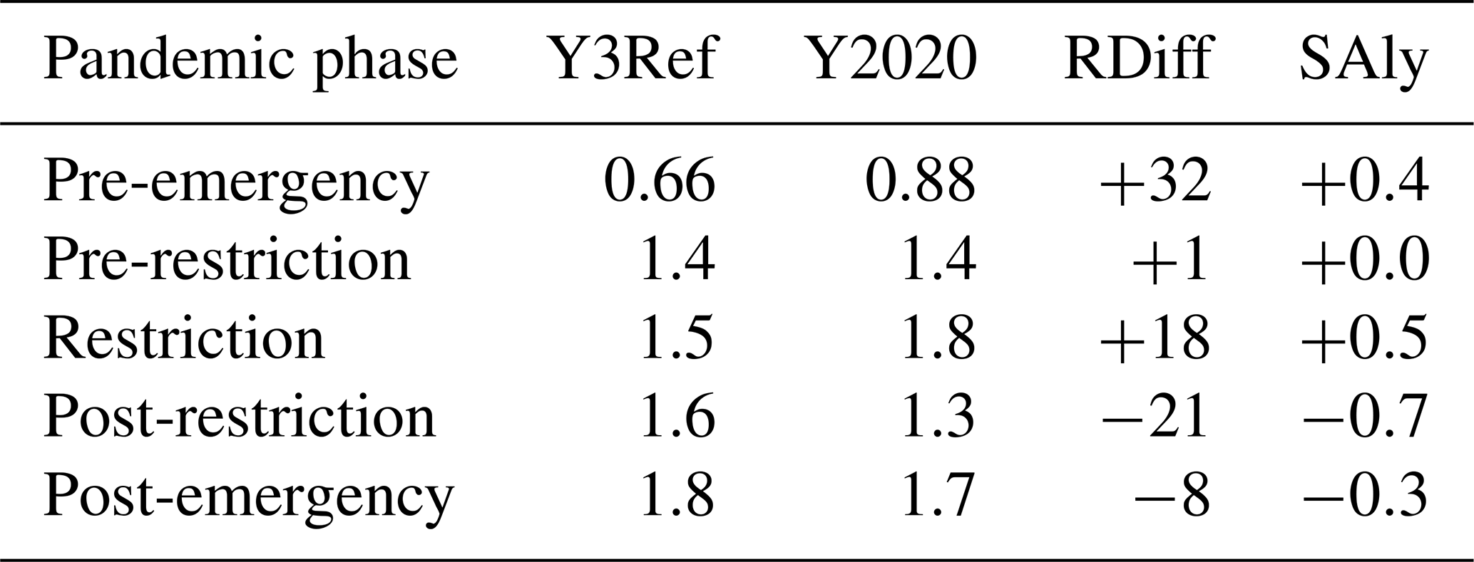
An overview of the major meteorological data during the whole state of emergency interval (98 d) is summarised in Table S2. The drought did not seem to influence substantially the WS and GRad but affected considerably the RH and indirectly the PBLH_max. The alterations in the PBLH_max in the average reference year and year 2020 over the pandemic phases are, therefore, quantified separately in Table 1 and are also displayed in Fig. S2. The time series for WS and T are also given in Figs. S3 and S4, respectively. It is seen in Fig. S2 that the Restriction phase – which is of particular interest for this study – was influenced by the PBLH_max in a more-or-less persistent manner without larger oscillations or fluctuations. The RDiff properties are taken into consideration when quantifying the concentration changes (Sect. 3.5). Lastly, it should also be mentioned that some of the differences in the meteorological data become small or insignificant when comparing them to their uncertainty intervals (in particular, for the modelled PBLH_max).

Table 1 Medians of the daily maximum planetary boundary layer height (km) in the average reference year comprising 2017–2019 (Y3Ref) and year 2020 (Y2020) together with their relative difference (RDiff) in % and their anomaly standardised to SD (SAly) over the five consecutive phases of the first COVID-19 outbreak.

3.2 Motor vehicle road traffic

Time series of vehicle flow on a major route (Váci Road, site no. 2 in Fig. 1) over the time interval studied in the average reference year and year 2020 are shown in Fig. 2 as examples. The other urban sites exhibited very similar time behaviour and tendencies.

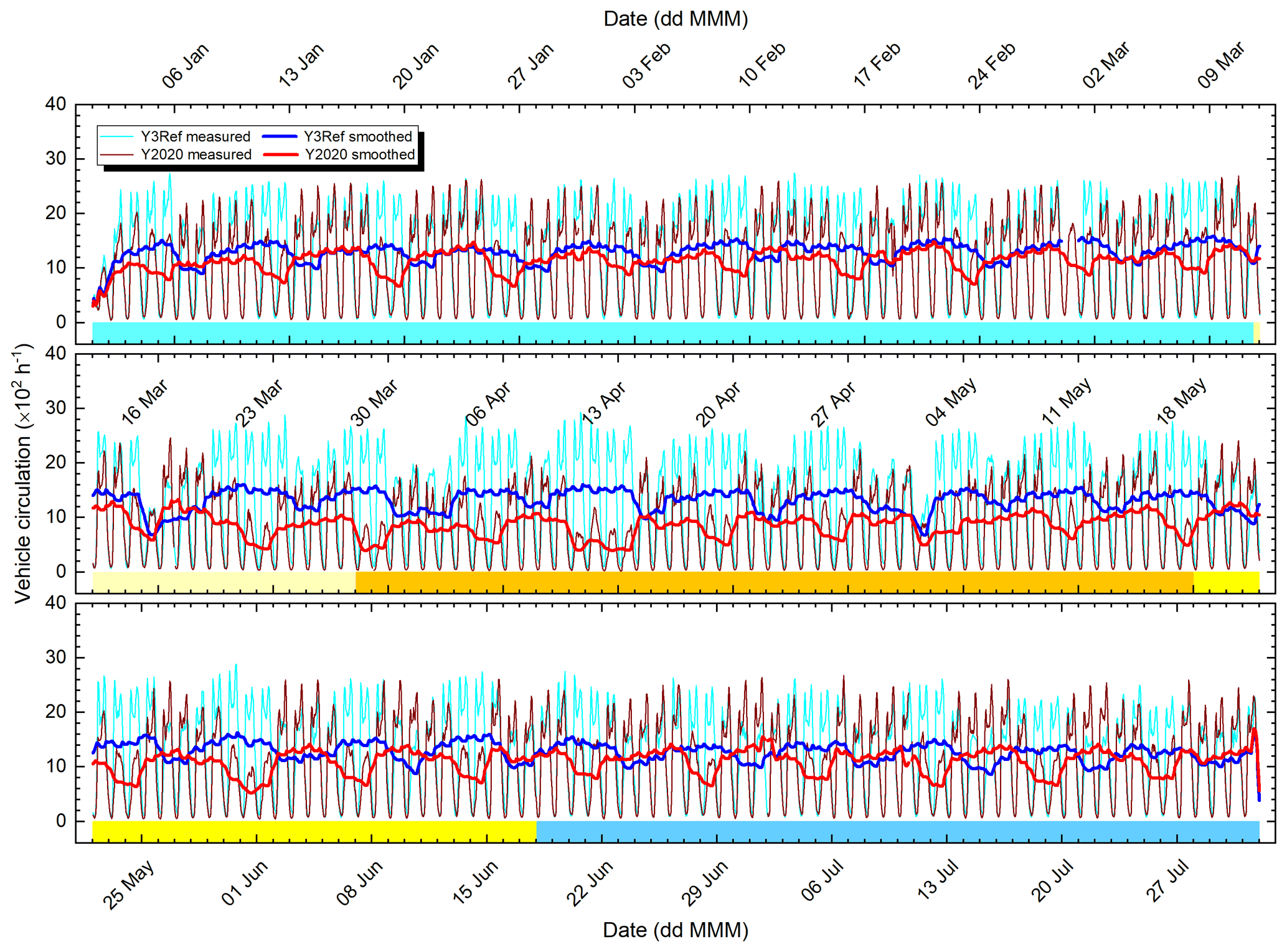
Figure 2 Time series of motor vehicle circulation on a major route (Váci Road) in Budapest in both directions in the average reference year comprising 2017–2019 (Y3Ref) and year 2020 together with their 24 h smoothed curves over the five consecutive phases of the first COVID-19 outbreak. The phases are marked by the following colour codes: Pre-emergency phase lighter blue, Pre-restriction phase lighter yellow, Restriction phase orange, Post-restriction phase darker yellow and Post-emergency phase darker blue. The tick labels of the abscissa indicate the Mondays in 2020.

The time series for vehicle flow showed a clear periodicity. On each workday, two peaks – corresponding to the early morning and late afternoon rush hours – can be identified. In addition to this periodicity, the smoothed curves also revealed an obvious cycling due to a repeated workdays and holidays sequence. More importantly, the time series implied that in the Pre-emergency pandemic phase, the road traffic in the city centre in Y2020 was very similar to that in Y3Ref. The difference only appeared as a horizontal shift in time, which was caused by the occurrence of holidays in the average reference year and year 2020. Two weeks before the introduction of the restriction on movement, the vehicle circulation already started declining, and in the last week of the Pre-restriction phase, it already reached the level observed later in the Restriction phase. During these 8 or 9 weeks, the vehicular circulation on workdays was around the ordinary levels on holidays in 2017–2019. The circulation approached its ordinary values within or after the first week of the Post-restriction phase step-wisely. After that, the curves for the 2 years were at almost identical levels again. The changes in the vehicle flow are quantified in Sect. 3.5 together with the pollutant concentrations.

The shapes of the diurnal patterns (Fig. S5) for the average reference year and year 2020 were similar to each other, with some modifications. Differences could be identified in the Pre-restriction and Restriction pandemic phases between 16:00 and 19:00, when the traffic flow on weekends seemed to be systematically and in excess lower in 2020 than in the average reference year. This could be due to the limitations on shopping and to modified going-out routines of inhabitants under the restrictions. Similarly, the early morning peak on workdays in the Post-emergency (and partly Post-restriction) phases was smaller in excess in Y2020 than in Y3Ref, which can likely be linked to fewer people going physically to work due to propagated home-office jobs. To facilitate the comparison of diurnal patterns of vehicle circulation and of atmospheric concentrations, the plot showing the diurnal variation of concentrations in the Restriction phase was extended by the vehicle flow in the same pandemic phase (Fig. 7).

3.3 Time series of concentrations

Time series of NO, O₃, PM_2.5 mass and N_6–1000 atmospheric concentrations over the time interval studied are shown in Figs. 3–6, respectively. The chemical species selected represent primary pollutant gases, secondary pollutant gases and two different aerosol properties, respectively. The corresponding curves for NO₂, CO, SO₂, PM₁₀ mass and N_100–1000 are displayed in Figs. S6–S10, respectively.

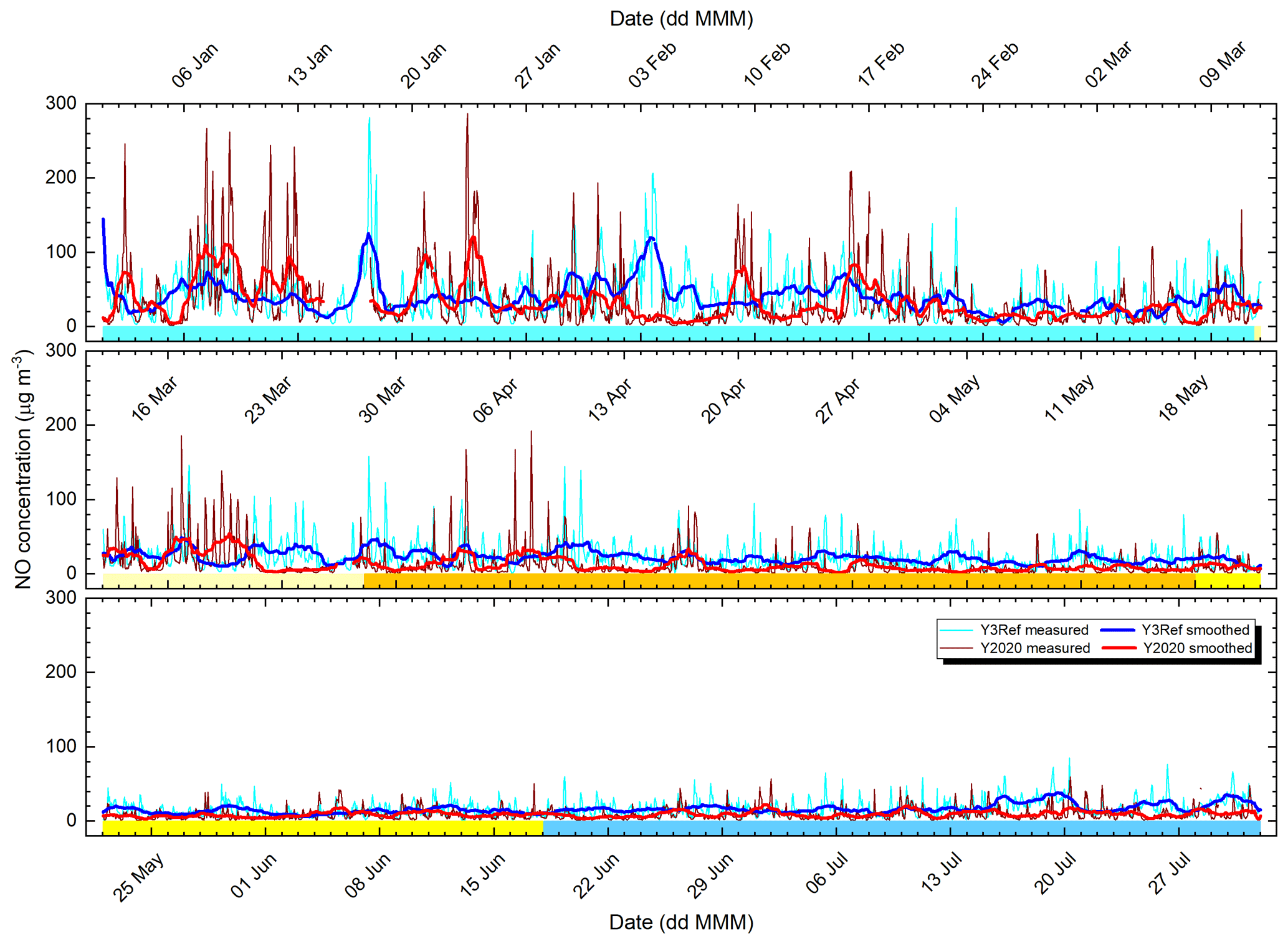
Figure 3 Time series of NO concentration in the average reference year comprising 2017–2019 (Y3Ref) and year 2020 together with their 24 h smoothed curves over the five consecutive phases of the first COVID-19 outbreak. The phases are marked by the following colour codes: Pre-emergency phase lighter blue, Pre-restriction phase lighter yellow, Restriction phase orange, Post-restriction phase darker yellow and Post-emergency phase darker blue. The tick labels of the abscissa indicate the Mondays in 2020.

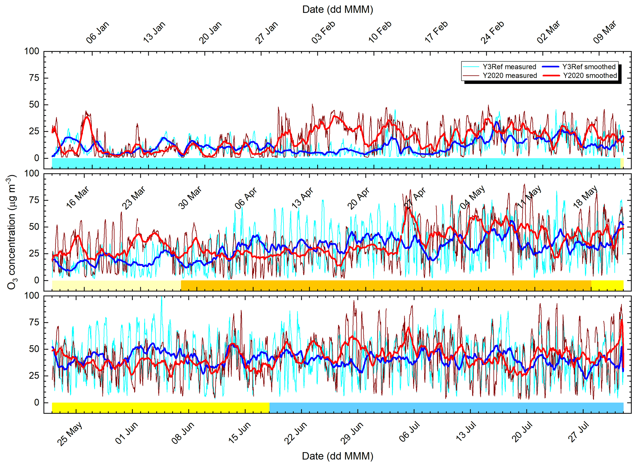
Figure 4 Time series of O₃ concentration in the average reference year comprising 2017–2019 (Y3Ref) and year 2020 together with their 24 h smoothed curves over the five consecutive phases of the first COVID-19 outbreak. The phases are marked by the following colour codes: Pre-emergency phase lighter blue, Pre-restriction phase lighter yellow, Restriction phase orange, Post-restriction phase darker yellow and Post-emergency phase darker blue. The tick labels of the abscissa indicate the Mondays in 2020.

Figure 5 Time series of PM_2.5 mass concentration in the average reference year comprising 2017–2019 (Y3Ref) and year 2020 together with their 24 h smoothed curves over the five consecutive phases of the first COVID-19 outbreak. The phases are marked by the following colour codes: Pre-emergency phase lighter blue, Pre-restriction phase lighter yellow, Restriction phase orange, Post-restriction phase darker yellow and Post-emergency phase darker blue. The tick labels of the abscissa indicate the Mondays in 2020.

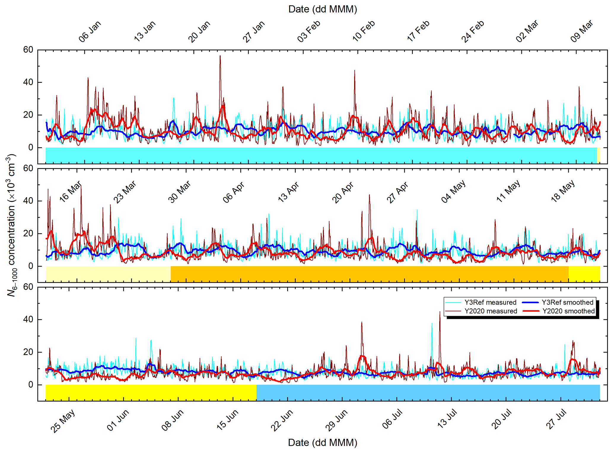
Figure 6 Time series of N_6–1000 concentration in the average reference year comprising 2017–2019 (Y3Ref) and year 2020 together with their 24 h smoothed curves over the five consecutive phases of the first COVID-19 outbreak. The phases are marked by the following colour codes: Pre-emergency phase lighter blue, Pre-restriction phase lighter yellow, Restriction phase orange, Post-restriction phase darker yellow and Post-emergency phase darker blue. The tick labels of the abscissa indicate the Mondays in 2020.

The curves for both measured and smoothed data demonstrated that the concentrations varied substantially in time. The changes on the smoothed curves seemed to be fluctuations on a daily scale and, for some pollutants, they appeared to exhibit some tendencies on a monthly scale, while the data series possessed diurnal periodicity as well. The trends, i.e. the smoothed curves over the 7 months, are in line with the distributions of the monthly median concentrations of the species at identical locations determined for several years (Salma et al., 2020b).

The annual relative SDs (RSDs) for NO, NO₂, CO, O₃, SO₂, PM₁₀ mass, PM_2.5 mass, N_6–1000, N_6–100, N_25–100 and N_100–1000 in year 2017–2019 were 115 %, 56 %, 43 %, 91 %, 37 %, 56 %, 74 %, 63 %, 69 %, 68 % and 68 %, respectively (cf. Sect. 1). Their time distributions were complex. For species which do not normally show seasonal tendency such as particle number concentrations and perhaps PM₁₀ mass, the distributions of monthly RSDs were also featureless. For SO₂, which tends to exhibit smaller concentration levels in summer than in winter, the distribution of its monthly RSDs seemed to have an opposite behaviour. For O₃, which exhibits larger concentrations in summer than in winter, the distribution of monthly RSDs showed again an opposite behaviour. These relationships are in accordance with general metrological expectations. Excitingly, for NO, NO₂, CO and perhaps PM_2.5 mass, the distributions of monthly RSDs appeared to roughly follow in parallel the concentration trends within the concentration ranges actually obtained. The largest decrease in the RSDs from winter to summer was observed for NO, which was approximately 20 % (of its annual mean RSD). The latter association could likely be linked to meteorological conditions and source/sink intensities of these pollutants.

Many chemical species investigated originate from rather different sources. Nevertheless, their atmospheric concentrations often changed coherently, particularly in winter and early spring. A nice example is the interval of approximately 14–28 March 2020 when most species varied consistently. The MCPs for these days indicate strong anticyclonic weather types over the Carpathian Basin and stagnant and relatively calm meteorological conditions without precipitation in the area (Fig. S1). It is a confirmation of the common effects of regional meteorology on atmospheric concentrations and that the daily evolution of meteorology can have a higher influence on atmospheric concentrations than the source intensities under such specific conditions (Salma et al., 2020a). Its consequences for the air quality are discussed in Sect. 3.8.

The curves for PM_2.5 mass and N_6–1000 confirmed that there is a weak association between these two types of aerosol metrics (de Jesus et al., 2019). They are connected mainly via meteorological properties, which is anyway active for all pollutants. It was sensible, therefore, that both types of aerosol concentrations were included in the study as separate variables.

3.4 Diurnal variations

Average diurnal variations of NO, O₃, SO₂, PM_2.5 mass and N_6–100 together with the vehicle circulation separately for workdays and holidays over the Restriction pandemic phase, for which the differences in the shapes are expected to be the largest, are shown in Fig. 7 as examples.

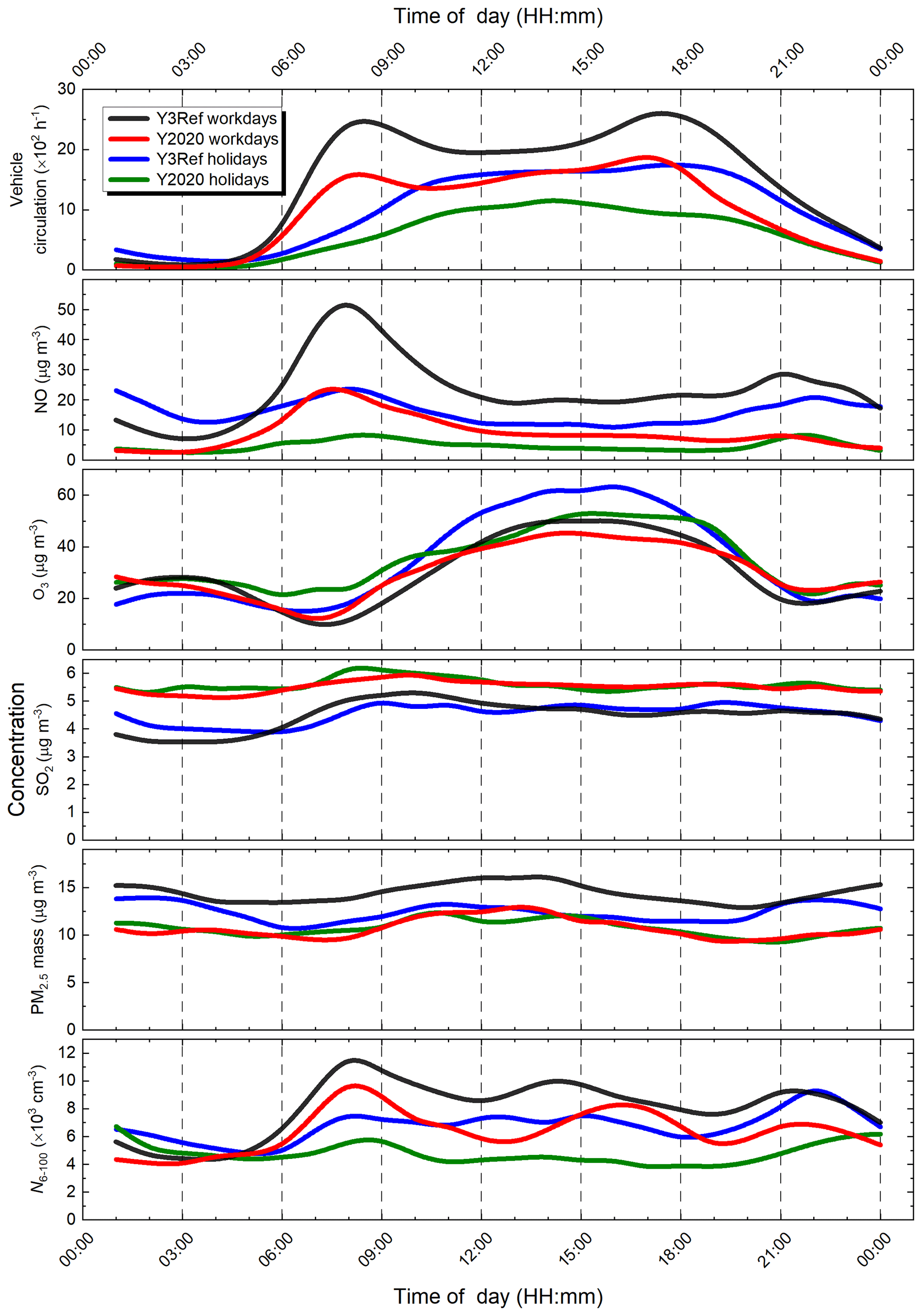
Figure 7 Average diurnal variations of motor vehicle road traffic in both directions on a major route (Váci Road) in Budapest and of NO, O₃, SO₂, PM_2.5 mass and N_6–100 concentrations separately for workdays and holidays in the average reference year comprising 2017–2019 (Y3Ref) and year 2020 during the Restriction phase of the first COVID-19 outbreak.

The curves of NO and N_6–100 (together with NO₂, CO and N_6–1000, which are not shown) followed the typical pattern of road traffic. They can largely be associated with vehicular sources (tailpipe emissions, primary and secondary particles) and can advantageously be applied for assigning potential concentration changes to traffic reduction. It is seen that their morning peak coincided with the peak of the morning rush hour, while their evening peak appeared later than the peak of the afternoon rush hour. This shift could likely be related to the daily evolution and cycling of the PBLH and to mixing intensity. The curves of N_6–100 contained in addition the characteristic midday peak, which is caused by atmospheric NPF events. It is worth realising that its position was shifted to a later time. There were only nine quantifiable NPF events during the Restriction phase in year 2020, which might not result in a representative shape. An alternative explanation could be that this peak was caused by the overlapping effects of direct traffic emissions and NPF events superimposed on each other. This experimental observation should definitely be investigated and clarified when the necessary data sets become available.

The curves for O₃ seemed to be opposite to NO as far as both their daily variations and the orders of concentration magnitudes on workdays and holidays are concerned. These are in line with the understanding of their atmospheric processes and coupled reaction mechanisms (Jacob, 1999). In addition, the shapes in Y2020 seemed to be flattened with respect to Y3Ref. The O₃ curves were also affected by the clock change, since the concentrations of O₃ are substantially influenced by solar radiation.

The curves for SO₂ (together with PM₁₀ mass and N_100–1000, which are not shown) tracked the traffic pattern very loosely if at all. They could partially be related to traffic through diesel fuel, resuspension of urban dust by moving vehicles, dispersion of road surfaces, (non-exhaust) emissions from material wear of moving parts of vehicles and growth/ageing of exhausted particles from vehicles (Salma and Maenhaut, 2006). Additional changes in the shape of the time variation of SO₂ could be caused by altered heating of and cooking at homes due to the spreading practice of working from home.

There was no obvious connection between the traffic and PM_2.5 mass, which confirms our earlier conclusion that the fine particles in Budapest mainly originate from non-vehicular sources (Salma et al., 2020a).

3.5 Quantification of concentration changes

There are several mathematical statistical tests to determine whether atmospheric concentrations over some time intervals in different years belong to the same distribution or not. These methods, however, quantify the joint influence of all environmental effects (Sect. 1) and do not provide information on their causal relationships. The method described and applied below allows us to unfold some potential confounding influence of environmental variables (e.g. PBLH) from concentration changes in order to gain a closer insight into the source intensities of motor vehicles.

Median concentrations of pollutant gases and aerosol particles, median traffic circulation data together with their relative differences and standardised anomaly values for the five pandemic phases in the average reference year and year 2020 are summarised in Tables 2–6. It should be noted that the standardised anomalies are rather small when recalling, for instance, the rigorous concept of the limits of detection (3 × SD) and determination (10 × SD) in analytical chemistry. This is largely caused by the strong dynamic features of related atmospheric properties and processes (Sects. 1 and 3.3).

We showed in Sect. 3.1 that it is the PBLH_max of the meteorological conditions that likely caused the largest side effects on the concentrations, and, therefore, its influence was taken into account. A change in median concentrations for a pandemic phase was quantified to be significant if both its relative difference fell outside the band of [$\pm \mathrm{10}-f_{\mathrm{mix}}\times \mathrm{RDiff}\left({\mathrm{PBLH}}_{max}\right)$] % and its SAly was outside the range of ±0.3. The multiplication factor f_mix accounts for non-homogeneous mixing of pollutants within the boundary layer and for the effects of the daily PBLH evolution. It was roughly estimated to be approximately 0.5. Its negative sign expresses that atmospheric concentrations vary in a reciprocal manner with PBLH. The selected criteria were based upon exercises with the data in the individual years 2017, 2018 and 2019. The procedure represents a sensible and consequent approach, though alternative limits could also be set.

The Pre-emergency phase (Table 2) fitted completely into the heating season. The traffic flows in the city centre were identical, except for Váci Road, where they were somewhat lower in Y2020 than in Y3Ref. This could be caused by some local traffic arrangements. The PBLH_max increased by 32 % (Table 1), which is substantial and affected the concentrations. Most concentration changes were not significant. The exceptions were NO, O₃, PM₁₀ mass and PM_2.5 mass, and the latter two exhibited the largest anomalies. These two species have multiple sources. Organic matter and elemental carbon, for instance, make up approximately 35 % of the PM_2.5 mass in winter (Salma et al., 2020a), and biomass burning is the major source of carbonaceous aerosol in this season, with an approximate relative contribution to the total carbon of 67 %. The share of fossil-fuel combustion is around 25 %. This all implies that PM_2.5 mass concentrations can fluctuate extensively and irregularly in the heating season due to the source intensities. The reductions could also be related to changes in further meteorological properties such as T (mild February 2020, Fig. S4) or larger WS that acted on a shorter timescale than the pandemic phase (Fig. S3).

Table 2 Median atmospheric concentrations of NO, NO₂ (both in units of µg m⁻³), CO (mg m⁻³), O₃, SO₂, PM₁₀ mass, PM_2.5 mass (all in µg m⁻³), N_6–1000, N_6–100, N_25–100, N_100–1000 (all in 10³ cm⁻³) and median vehicle road traffic (h⁻¹) on Szabadság Bridge, Váci Road, Széna Square and Alkotás Road in the average reference year comprising 2017–2019 (Y3Ref) and year 2020 together with their relative difference (RDiff, %) and their anomaly standardised to SD (SAly) for the Pre-emergency phase of the first COVID-19 outbreak. Chemical species with significant change are shown in bold.

The higher O₃ concentration could partly be associated with the lower concentrations of NO. Ozone exhibits a strong seasonal dependency (Salma et al., 2020b). Lower concentrations in winter and early spring can be easily disturbed by their non-linear chemistry and by high WS. The modest SAly for O₃ suggests that this considerable relative concentration increase was mostly a consequence of low levels of O₃ in winter. The case nicely demonstrates the strength of and requirement for the coupled utilisation of RDiff and SAly criteria. Furthermore, the main differences in the concentrations appeared sporadically in an isolated manner. In addition, there was no coherence among the traffic-related variables. Therefore, all significant variations were interpreted as results of inter-annual variability in local meteorology, emissions and formation processes.

The Pre-restriction phase (Table 3) was rather short (16 d), and, therefore, its interpretation should be approached with special caution due to some issues in representativity. It was also completely part of the heating season, and the extreme drought in the Carpathian Basin in 2020 could also play a role. The PBLH_max was almost identical in both years (Table 1). The concentrations of NO₂, PM_2.5 mass and perhaps NO declined, while O₃ was enhanced. Excitingly, CO did not show a substantial decrease. The changes could be affected by lower traffic during its last half/week (Fig. 2) and increased GRad.

Table 3 Median atmospheric concentrations of NO, NO₂ (both in units of µg m⁻³), CO (mg m⁻³), O₃, SO₂, PM₁₀ mass, PM_2.5 mass (all in µg m⁻³), N_6–1000, N_6–100, N_25–100, N_100–1000 (all in 10³ cm⁻³) and median vehicle road traffic (h⁻¹) on Szabadság Bridge, Váci Road, Széna Square and Alkotás Road in the average reference year comprising 2017–2019 (Y3Ref) and year 2020 together with their relative difference (RDiff) in % and their anomaly standardised to SD (SAly) for the Pre-restriction phase of the first COVID-19 outbreak. Chemical species with significant change are shown in bold.

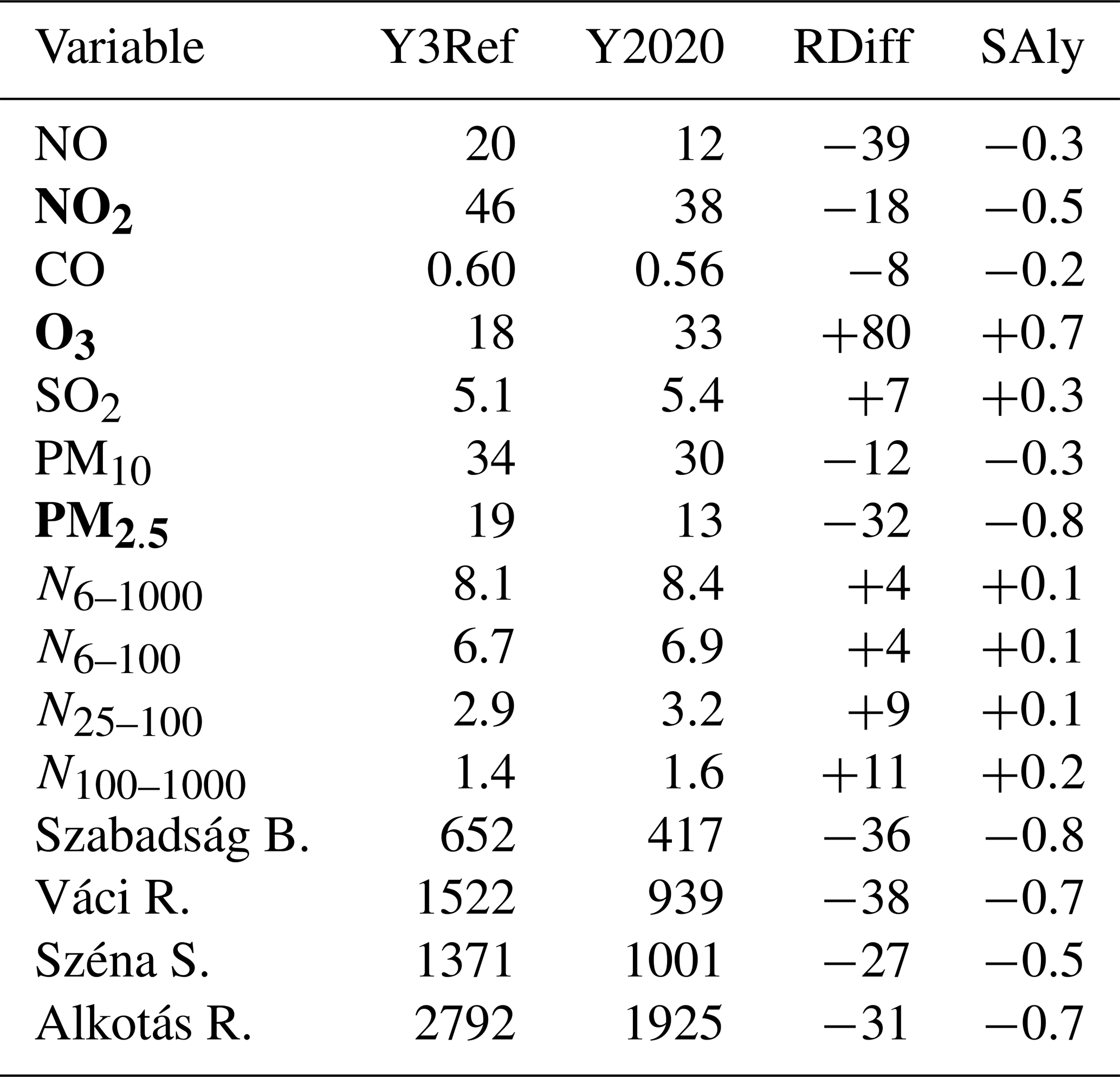
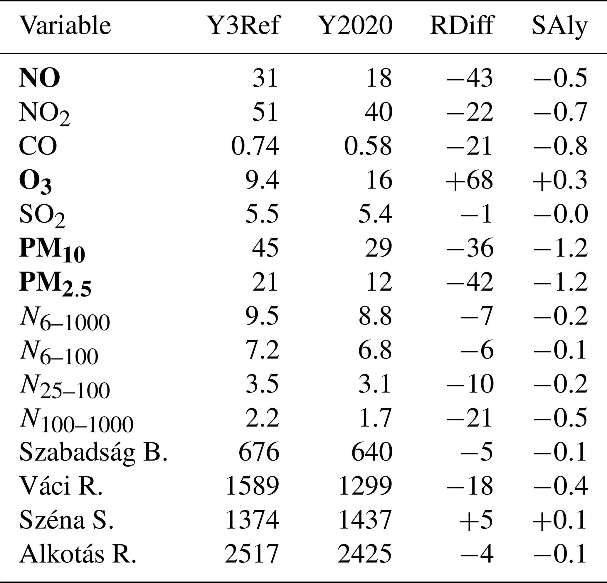
The beginning one-third part of the Restriction phase (Table 4) fell in the heating season, and it was fully incorporated into the extremely dry weather season. The vehicle flows were reduced by approximately half uniformly at all urban locations. Concentrations of NO, NO₂, CO, PM_2.5 mass, N_6–1000 and N_6–100 changed significantly, and they all declined. The alterations happened in a systematic or continuous manner in time (Figs. 2–6, S6 and S7). These species can be associated with vehicular road traffic, except for PM_2.5 mass, which is linked more to household and residential sources. At the same time, some other important pollutants such as N_100–1000 or SO₂ – which are typically related to larger spatial extent or region and which could, therefore, be influenced by meteorology – did not change significantly. Similar reductions were reported for other urban locations in the world (Keller et al., 2020; Lal et al., 2020; Le et al., 2020; Lee et al., 2020; Tobías et al., 2020). This all can be interpreted that the alterations in NO, NO₂, CO, N_6–1000 and N_6–100 concentrations were primarily caused by the lower vehicular traffic intensity in the city and that the PBLH could also contribute by approximately 9 % in an absolute sense (Table 1). The increased O₃ can be explained by its production primarily from volatile organic compounds (VOCs) and NO_x in the VOC-limited chemical regime even under decreasing NO_x conditions (Jacob, 1999; Lelieveld and Dentener, 2000). This regime is typical for many large cities, where the VOCs can involve, for instance, aromatics such as benzene and toluene, which largely originate from traffic sources.

Table 4 Median atmospheric concentrations of NO, NO₂ (both in units of µg m⁻³), CO (mg m⁻³), O₃, SO₂, PM₁₀ mass, PM_2.5 mass (all in µg m⁻³), N_6–1000, N_6–100, N_25–100, N_100–1000 (all in 10³ cm⁻³) and median vehicle road traffic (h⁻¹) on Szabadság Bridge, Váci Road, Széna Square and Alkotás Road in the average reference year comprising 2017–2019 (Y3Ref) and year 2020 together with their relative difference (RDiff) in % and their anomaly standardised to SD (SAly) for the Restriction phase of the first COVID-19 outbreak. Chemical species with significant change are shown in bold.

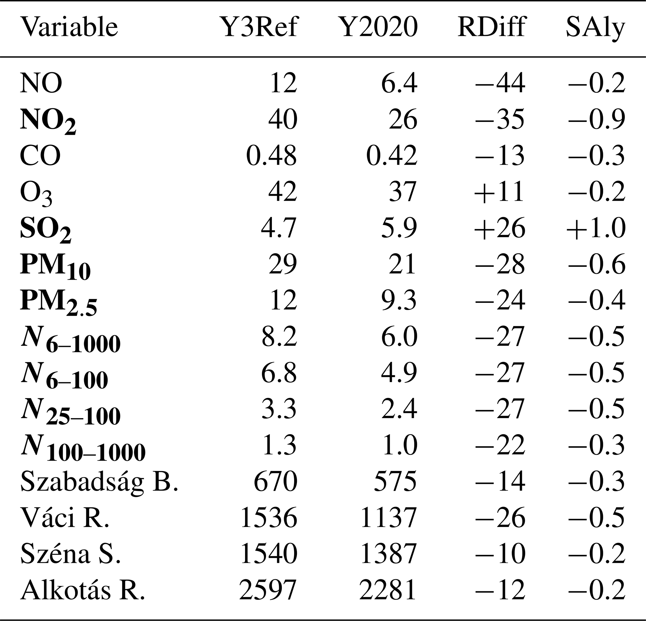
In the Post-restriction phase (Table 5), the vehicle flow recovered step-wisely. The PBLH_max in Y2020 decreased substantially relative to Y3Ref (Table 1). Most chemical species such as NO₂, SO₂, PM₁₀ mass, PM_2.5 mass, N_6–1000, N_6–100, N_25–100 and N_100–1000 exhibited significant changes. The list also included variables which characterise the region. At the same time, some typical vehicular-related species such as NO and CO – which are not really water-soluble – were not among them. Most significant changes showed decreasing tendency, except for SO₂, which increased. The latter was caused by a continuously increasing SO₂ concentration (Fig. S8) recorded at the other air quality monitoring stations as well. The increase was likely caused as a perturbance by some local sources in the upwind direction from the city. This all suggests that the alterations were mainly produced by arrival of continued and spatially extended rains in the second half of the pandemic phase (Fig. S1). The precipitation washed out many chemical species from the urban and regional atmospheres. This time interval unambiguously demonstrated that the regional weather can cause similar modifications in atmospheric concentrations as substantially reduced (by 50 %) urban traffic.

Table 5 Median atmospheric concentrations of NO, NO₂ (both in units of µg m⁻³), CO (mg m⁻³), O₃, SO₂, PM₁₀ mass, PM_2.5 mass (all in µg m⁻³), N_6–1000, N_6–100, N_25–100, N_100–1000 (all in 10³ cm⁻³) and median vehicle road traffic (h⁻¹) on Szabadság Bridge, Váci Road, Széna Square and Alkotás Road in the average reference year comprising 2017–2019 (Y3Ref) and year 2020 together with their relative difference (RDiff) in % and their anomaly standardised to SD (SAly) for the Post-restriction phase of the first COVID-19 outbreak. Chemical species with significant change are shown in bold.

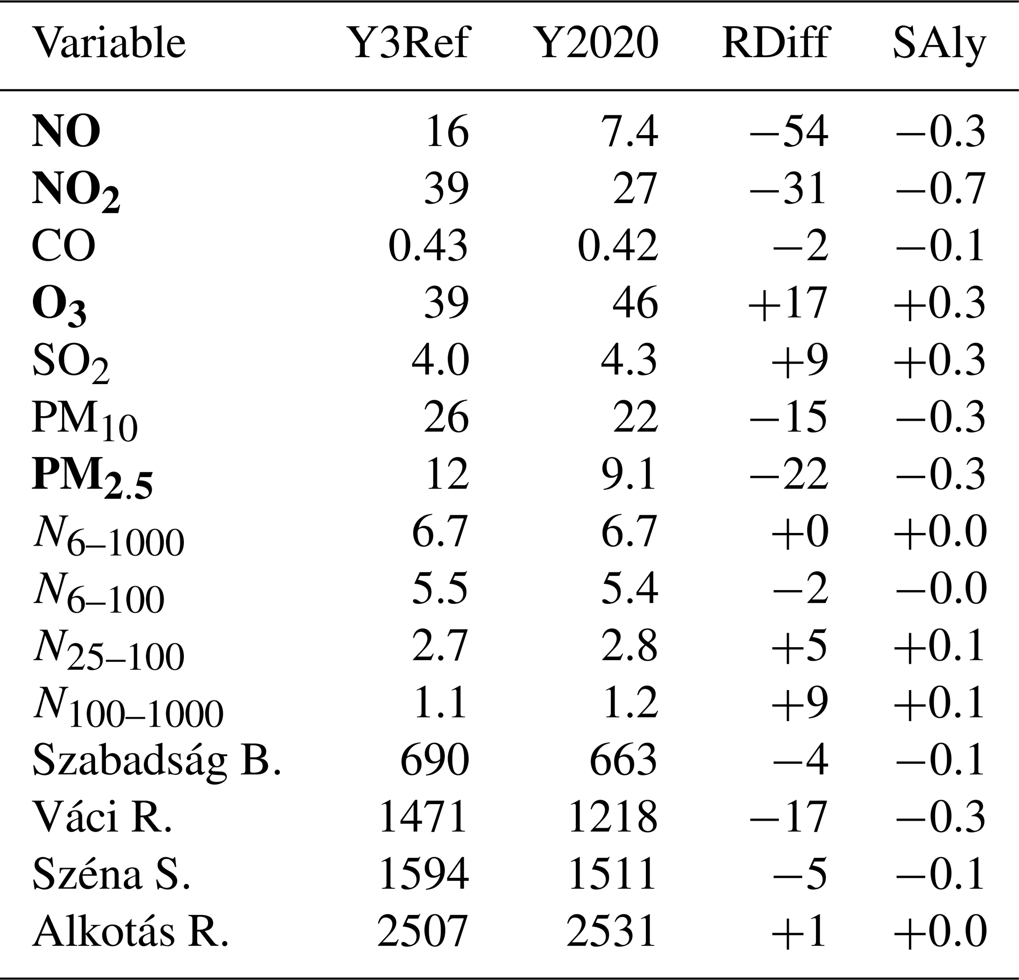
In the Post-emergency phase (Table 6), the traffic was at its ordinary level and there were no larger weather alternations. Most concentrations – including some major vehicle-related pollutants such as CO and N_6–100 – did not change significantly. The exceptions were NO, NO₂, O₃ and PM_2.5 mass. The first three variables are connected to each other through atmospheric chemistry. The changes can likely be linked to inter-annual variability in sources, sinks, meteorological properties that act on a shorter timescale than the pandemic phase and atmospheric transformation and transport – similarly to that observed in the Pre-emergency phase.

Table 6 Median atmospheric concentrations of NO, NO₂ (both in units of µg m⁻³), CO (mg m⁻³), O₃, SO₂, PM₁₀ mass, PM_2.5 mass (all in µg m⁻³), N_6–1000, N_6–100, N_25–100, N_100–1000 (all in 10³ cm⁻³) and median vehicle road traffic (h⁻¹) on Szabadság Bridge, Váci Road, Széna Square and Alkotás Road in the average reference year comprising 2017–2019 (Y3Ref) and year 2020 together with their relative difference (RDiff) in % and their anomaly standardised to SD (SAly) for the Post-emergency phase of the first COVID-19 outbreak. Chemical species with significant change are shown in bold.

3.6 Change rates

Linear regression analysis between the median RDiff for vehicle traffic on one side and RDiff for pollutants corrected for the RDiff(PBLH_max) on the other side for all pandemic phases yielded change rates and SDs for NO, NO₂, N_6–1000 and CO of 0.63 ± 0.23, 0.57 ± 0.14, 0.40 ± 0.17 and 0.22 ± 0.08, respectively. For PM₁₀ mass and PM_2.5 mass, the rates were slightly negative and insignificant. The data points for the Post-restriction phase – which were substantially affected by precipitation and frontal weather systems – were excluded from this analysis.

The change rates suggest that nitrogen oxides vary sensitively with traffic, total particle number concentration shows considerable dependency, while variation of CO is modest. This is linked to their residence times as well. The PM mass concentrations do not appear to be closely related to traffic intensity in central Budapest.

3.7 Spatial gradients

Spatial distributions of NO and O₃ derived by CAMS ensemble reanalysis in 2018–2019 and 2020 during the Restriction pandemic phase are shown in Figs. 8 and 9 as examples. The absolute concentrations can be different from the measured values due to the specialities in the applied models, while the relative tendencies are expected to be expressed correctly. Figure 8 indicates that the differences from the corresponding median (spatial gradients) in 2020 were larger than in 2018–2019. This can be explained if the relative concentration changes at the outer parts of the city or near-city background were even larger than in the centre. The spatial distribution of NO₂ was similar to NO, although its gradients were smaller than for NO. Spatial distributions of CO and PM_2.5 mass were featureless and similar to each other in 2018–2019 and 2020.

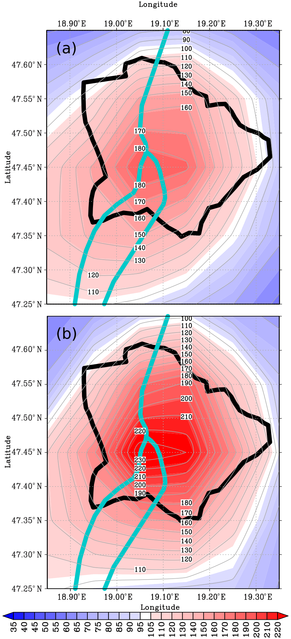
Figure 8 Spatial distribution of median NO concentration in Budapest in 2018–2019 (a) and 2020 (b) during the Restriction phase of the first COVID-19 outbreak obtained from CAMS ensemble reanalysis. The concentrations were normalised to the overall spatial median concentrations of 0.93 and 0.59 µg m⁻³, respectively. The border of the city and the Danube River are indicated with curves in black and blue colours, respectively, for better orientation.

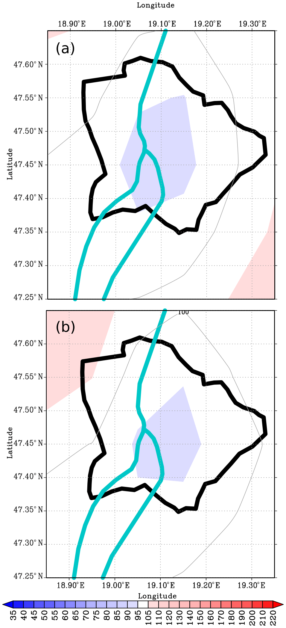
Figure 9 Spatial distribution of median O₃ concentration in Budapest in 2018–2019 (a) and 2020 (b) during the Restriction phase of the first COVID-19 outbreak obtained from CAMS ensemble reanalysis. The concentrations were normalised to the overall spatial median concentrations of 60 and 67 µg m⁻³, respectively. The border of the city and the Danube River are indicated with curves in black and blue colours, respectively, for better orientation.

Spatial distributions of O₃ (Fig. 9) and, perhaps, SO₂ (which is not shown) exhibited relative decrease in the centre, whose gradients were relatively small and similar to each other for both time intervals. This all is in line with the tendencies observed in their measured concentrations (Sect. 3.3 and 3.4). We are aware that several pollutants originate from diffusive line sources, which can be enriched along roads and, therefore, much larger concentration gradients can occur on smaller spatial scales.

3.8 Potentials for improving air quality

In order to assess the importance of concentration changes that could be achieved by tranquilising the vehicle road traffic in Budapest, the atmospheric concentrations and their possible decrements were compared to various limit values (EU Directives, 2008; VM 4, 2011).

NO₂ exhibited the most frequent exceedances of standards for the protection of health. Its concentrations in 2017, 2018 and 2019 were larger in 172, 155 and 61 cases than the 1 h national health limit of 100 µg m⁻³ (Fig. S6). The permitted number of exceedances is 18 a year. It is mentioned that this concentration limit is 200 µg m⁻³ for the EU, which would be fulfilled completely. The NO₂ excess usually remained modest – particularly when contrasted with the smog alert thresholds of 350 (for the warning state) and 400 µg m⁻³ (for the alarm state). The daily health limit of 85 µg m⁻³ was also exceeded in 6, 2 and 0 d in the 3 years, respectively. A reduction of 10 % in vehicle circulation (that corresponds to a 6 % decline in NO₂ concentration) would decrease the number of exceedances of the 1 h national health limit to 114, 98 and 42, respectively (thus, typically by ca. 30 %), while the number of days above the daily health limit would be lowered to 2, 0 and 0, respectively.

Less frequent though more severe exceedances than for NO₂ happened for PM₁₀ mass (Fig. S9). The daily mean PM₁₀ mass concentrations in 2017, 2018 and 2019 exceeded the daily health limit of 50 µg m⁻³ in 36, 93 and 57 d, respectively, at this actual air quality monitoring station. Most exceedances occurred in the heating season. Their permitted number is 35 a year. The smog alert thresholds for the warning and alarm states are 75 and 100 µg m⁻³, respectively. The numbers of exceedances for the warning stage were 12, 17 and 9, respectively. It should be added that smog alerts are announced on the basis of a complex set of conditions which include larger numbers of monitoring stations and days. As a matter of fact, the warning state was announced three times for 11 d in total and once for 2 d in 2017 and 2018, respectively. There was no smog alert in 2019. It is stressed that all alarm states since 2007 were announced exclusively because of high PM₁₀ mass concentrations, and all alert intervals were confined to winter. This points to the role of local and regional meteorology and other sources than vehicle traffic (Salma et al., 2020a). There is a cold air pool that develops from time to time above the Carpathian Basin in winter, which generates a lasting T inversion and a shallow planetary boundary layer, restricts the vertical mixing and results in poor air quality over extended areas of the basin in larger and smaller cities as well as in rural areas.

All O₃ concentrations were below the maximum daily 8 h health limit of 120 µg m⁻³ (Fig. 4). The concentrations of CO were far away from both the 1 h and maximum daily 8 h health limits of 10 and 5 mg m⁻³, respectively (Fig. S7), and the situation was similar for SO₂, for which the 1 h and daily limits are 250 and 125 µg m⁻³, respectively (Fig. S8).

4 Conclusions

The relationships between urban air quality and motor vehicle road traffic are not straightforward since the contributions of traffic flow to pollutant concentrations are superimposed in the variability in local meteorological conditions, long-range transport of air masses and other sources/sinks. We introduced here an approach based on both relative difference and standardised anomaly, which helps unfold some important confounding environmental factors. It can support the creation of a generalised picture on urban atmospheres.

The method was deployed on the Budapest data during the different phases of the first COVID-19 outbreak. Various restriction measures introduced due to the pandemic resulted in a decline of vehicle road traffic down to approximately 50 % during the severest limitations. In parallel, concentrations of NO, NO₂, CO, N_6–1000 and N_6–100 decreased substantially, some other species such as PM_2.5 mass, PM₁₀ mass and N_100–1000 changed modestly and inconclusively, while O₃ showed an increasing tendency. Change rates of NO and NO₂ with relative change in traffic intensity were the largest (approximately 0.6), total particle number concentration showed considerable dependency (0.4), while variation of CO was modest (0.2). It was demonstrated that a similar decrease in concentrations as observed in the strictest pandemic phase can also be caused by other (natural/meteorological) effects than traffic. The rainy weather in June 2020 (the so-called St. Medard's 40 d of rain in central European folklore) yielded, for instance, very similar low pollution levels.

The study revealed that intentional reduction of traffic intensity can have unambiguous potentials for improving urban air quality as far as NO, NO₂, CO and particle number concentrations are concerned. It should be added that the most critical pollutant in many European cities, including Budapest, namely the PM₁₀ mass, however, did not seem to be considerably affected by vehicle flow. Nevertheless, measures for tranquillising urban traffic can contribute to improved air quality through a new strategy for lowering the population exposure of inhabitants instead of high-risk management of individuals.

The method could be expanded by other important ordinary chemical species such as soot and by other location types such as near-city or regional background sites jointly with central locations in order to obtain more exact meteorology-normalised changes. The results also point to the importance of non-linear relationships among precursors and secondary pollutants, which are to be further studied to gain better insights into urban atmospheric chemistry and air quality issues.