the Creative Commons Attribution 4.0 License.
the Creative Commons Attribution 4.0 License.
 | 17 Dec 2020
Measurements to determine the mixing state of black carbon emitted from the 2017–2018 California wildfires and urban Los Angeles
Joseph Ko
Trevor Krasowsky
The effects of atmospheric black carbon (BC) on climate and public health have been well established, but large uncertainties remain regarding the extent of the impacts of BC at different temporal and spatial scales. These uncertainties are largely due to the heterogeneous nature of BC in terms of its spatiotemporal distribution, mixing state, and coating composition. Here, we seek to further understand the size and mixing state of BC emitted from various sources and aged over different timescales using field measurements in the Los Angeles region. We measured refractory black carbon (rBC) with a single-particle soot photometer (SP2) on Catalina Island, California (∼70 km southwest of downtown Los Angeles) during three different time periods. During the first campaign (September 2017), westerly winds were dominant and measured air masses were representative of well-aged background over the Pacific Ocean. In the second and third campaigns (December 2017 and November 2018, respectively), atypical Santa Ana wind conditions allowed us to measure biomass burning rBC (BCbb) from air masses dominated by large biomass burning events in California and fossil fuel rBC (BCff) from the Los Angeles Basin. We observed that the emissions source type heavily influenced both the size distribution of the rBC cores and the rBC mixing state. BCbb had thicker coatings and larger core diameters than BBff. We observed a mean coating thickness (CTBC) of ∼40–70 nm and a count mean diameter (CMD) of ∼120 nm for BCbb. For BCff, we observed a CTBC of ∼5–15 nm and a CMD of ∼100 nm. Our observations also provided evidence that aging led to an increased CTBC for both BCbb and BCff. Aging timescales < ∼1 d were insufficient to thickly coat freshly emitted BCff. However, CTBC for aged BCff within aged background plumes was ∼35 nm thicker than CTBC for fresh BCff. Likewise, we found that CTBC for aged BCbb was ∼18 nm thicker than CTBC for fresh BCbb. The results presented in this study highlight the wide variability in the BC mixing state and provide additional evidence that the emissions source type and aging influence rBC microphysical properties.
- Article
(21433 KB) - Full-text XML
-
Supplement
(32908 KB) - BibTeX
- EndNote


Atmospheric black carbon (BC) is a carbonaceous aerosol that can result from the incomplete combustion of carbon-containing fuels. Major energy-related sources of BC include vehicular combustion, power plants, residential fuel use, and industrial processes. Biomass burning, which can be either anthropogenic or natural, is another significant BC source. BC is a pollutant of particular interest for two main reasons: (1) it absorbs solar radiation, which results in atmospheric warming (Ramanathan and Carmichael, 2008), and (2) it is associated with increased risk of cardiopulmonary morbidity and mortality (World Health Organization, 2012). Regarding its effect on climate, BC is widely considered to be the second strongest contributor to climate warming, after carbon dioxide (Bond et al., 2013). Although it has been established that BC is a strong radiative forcing agent in Earth's atmosphere, considerable uncertainty remains regarding the extent to which BC affects Earth's radiative budget, from a regional to global scale (IPCC, 2013; Bond et al., 2013).
As the lifetime of BC is relatively short (∼ days to weeks), the spatiotemporal distribution of BC is highly heterogeneous and, thus, difficult to quantify (Krasowsky et al., 2018). The quantification of where and when BC is emitted around the world is also a challenging task that causes significant uncertainty (Bond et al., 2013). In addition to the difficulties that come with tracking the emission and distribution of BC, there are complex physical and chemical processes that govern the transformation of BC in the atmosphere, which ultimately impact its climate and health effects. These atmospheric processes, in addition to the emissions source type, influence the BC mixing state in a highly dynamic manner. A BC particle that is physically separate from other non-BC aerosol species is considered “externally mixed”. Conversely, BC is considered “internally mixed” if it is physically combined with another non-BC aerosol species (Bond et and Bergstrom, 2006; Schwarz et al., 2008a). As freshly emitted BC particles are transported in the atmosphere, they can obtain inorganic and organic coatings from gaseous pollutants that condense onto the BC, oxidation reactions on the BC surface, or the coalescence of other aerosol species onto the BC, making them more internally mixed (He et al., 2015). In general, the “mixing state” of BC describes the degree to which BC is internally mixed (Bond et al., 2013). The BC mixing state near the point of emission as well as the evolution of the mixing state during aging in the atmosphere can vary widely, depending on the source of emissions and atmospheric context.
An understanding of the evolution of the rBC mixing state as BC ages in the atmosphere is crucial for two reasons. First, it has been shown that non-refractory coatings on BC can enhance its absorption efficacy, implying that internally mixed BC with thick coatings can have a stronger warming potential in the atmosphere compared with uncoated or thinly coated BC (Moteki and Kondo, 2007; Wang et al., 2014). Second, coatings on BC can alter the aerosol's hygroscopicity and effectively shorten its lifetime by increasing the probability of wet deposition (McMeeking et al., 2011a; Moteki et al., 2012; Zhang et al., 2015). In short, freshly emitted BC particles are generally hydrophobic, but coatings acquired during the aging process can make BC-containing particles hydrophilic and, therefore, more susceptible to wet deposition. Thus, uncertainties in the evolution of the rBC mixing state directly translate to uncertainties regarding the impact of BC on Earth's climate due to both the radiative impact per particle mass and spatiotemporal variation of atmospheric BC loading.
Although there have been a number of laboratory experiments (Wang et al., 2018; He et al., 2015; Slowik et al., 2007; Knox et al., 2009) and field campaigns (Krasowsky et al., 2018; Metcalf et al., 2012; Cappa et al., 2012; Schwarz et al., 2008a) studying the rBC mixing state, there is considerable variability in results. For example, field studies in China suggest that the mass absorption cross section (MAC) of BC that has aged for more than a few hours should be enhanced by a factor of ∼2 (Wang et al., 2014), whereas other studies in California reported an absorption enhancement factor of ∼1.06 (Cappa et al. 2012) and ∼1.03 (Krasowsky et al., 2016). Preceding these studies, Bond and Bergstrom (2006) suggested an enhancement factor of ∼1.5 based on a review of laboratory and field studies. The wide range of reported values is not surprising given that the rBC mixing state is expected to be influenced by a variety of spatiotemporal factors such as source type, season, and regional atmospheric composition (Krasowsky et al., 2018). In other words, BC aged in different places and at different times may have significantly varying mixing states, resulting in a wide range of absorption and hygroscopicity enhancements in the real world.
Quantifying the BC mixing state is challenging because it requires single-particle analysis (Bond and Bergstrom, 2006). There are two main methods to measure the rBC mixing state: (1) microscopy (Johnson et al., 2005; Adachi et al., 2010, 2016) and (2) real-time, in situ measurements (Hughes et al., 2000). In our study, we quantify the rBC mixing state by taking real-time, in situ measurements with a single-particle soot photometer (SP2). The SP2 uses laser-induced incandescence to measure refractory black carbon (rBC) mass per particle, which can be used to directly compute the concentration, number concentration, and mass size distribution, and indirectly compute the number size distribution (Stephens et al., 2003). The SP2 can also measure the mixing state of rBC using one of two different methods. In the lag-time method, each sensed rBC-containing particle is deemed as either thinly coated or thickly coated using the measured time difference between the peak of the incandescence and scattering signals induced by the particle (Moteki and Kondo, 2007, 2008). In the leading-edge-only (LEO) method, the actual coating thickness for rBC-containing particles can be explicitly quantified (Gao et al., 2007). Further details regarding these two methods can be found in Sect. 2.3 and 2.4. In this study, we used both methods to quantify the rBC mixing state.
Table 1Major wildfires that were active during the three campaigns. Only the two largest fires from each campaign (in terms of burn area) are listed in the table below. Note that there were numerous other smaller fires that were active during the three campaigns, but they are not listed in this table.

* Data from the California Department of Forestry and Fire Protection (https://www.fire.ca.gov/incidents/, last access: 26 August 2019).
In this study, we measured rBC with an SP2 on Catalina Island, California (∼70 km southwest of Los Angeles) during three different time periods, with the goal of observing how the rBC loading and mixing state varied as a function of source type and source-to-receptor timescale. During the first campaign (September 2017), westerly winds dominated; thus, the sampling location was upwind of the dominant regional sources of rBC (i.e., urban emissions from the Los Angeles Basin). We suspect measurements during this period to represent well-aged particles; evidence suggests that some of the measured particles originated from wildfires in Oregon and northern California. In contrast, the second and third campaigns (December 2017 and November 2018, respectively) were dominated by northerly-to-easterly “Santa Ana conditions”, which advected fresh and aged rBC-containing particles from both biomass burning emissions and urban emissions. Several significant wildfires were active in the southern and northern California regions throughout the second and third campaigns. In particular, the Thomas Fire, which was active in southern California during the second campaign, was the second largest wildfire in modern California history. The Camp Fire, which was active in northern California during the third campaign, was the 16th largest fire in terms of burn area size and was also considered the deadliest and most destructive wildfire in modern Californian history. Table 1 lists the two most significant wildfires for each campaign period that impacted our rBC measurements, along with the total burn area and time period of non-containment for each fire. Mass and number concentrations of rBC-containing particles, rBC size distributions, the number fraction of thickly coated rBC-containing particles (i.e., using the lag-time method), and absolute coating thickness values (i.e., using the LEO method) are reported. We then evaluate how the rBC loading, size distribution, and mixing state relate to the meteorology and major sources at the time of measurements in order to further understand the microphysical transformation of BC as it ages in the atmosphere. While a few past studies have investigated the mixing state of rBC in the Los Angeles region using the SP2 (Metcalf et al., 2012; Cappa et al., 2012; Krasowsky et al., 2018), this study is the first to use fixed ground-based measurements off the coast of Los Angeles to focus on how both wildfire source-to-receptor travel time and wildfire versus urban emissions influence the rBC mixing state.
2.1 Measurement location and time periods
All measurements reported in this study were conducted at the USC Wrigley Institute for Environmental Studies on Catalina Island (∼33∘26′41.68′′ N, 118∘28′55.98′′ W). Catalina Island is located approximately 70 km (43.5 miles) southwest of downtown Los Angeles. Figure 1 shows the location of the sampling site relative to the Los Angeles metropolitan area. The three campaigns were conducted from 7 to 14 September 2017, 20 to 22 December 2017, and 12 to 18 November 2018, Pacific time (local time).
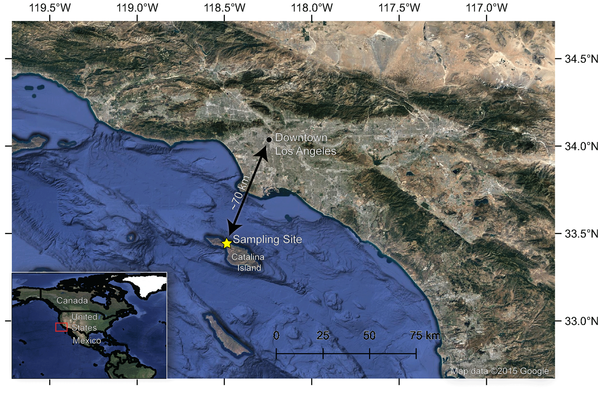
Figure 1Overview map showing the location of the sampling site with respect to the Greater Los Angeles (LA) area. Map data © Google Earth.
2.2 Instrumentation
An SP2 (Droplet Measurement Technologies, Boulder, CO) was used to quantify the physical characteristics of rBC-containing particles for all three campaigns. In short, the SP2 uses laser-induced incandescence to quantify rBC mass on a particle-by-particle basis. The SP2 uses a continuous Nd:YAG laser (λ=1064 nm) that is oriented perpendicular to the flow of air containing rBC-containing particles. As each particle passes through the intra-cavity laser, any coating on the rBC particle vaporizes while the core incandesces and emits thermal radiation. The scattered and thermally emitted radiation is measured by optical sensors and converted to signals that can then be used to obtain information about the mass and mixing state of the sampled rBC-containing particles. In this study, an assumed rBC density of 1.8 g cm−3 was used. The SP2 has detection limits from ∼0.5 to 50 fg rBC per particle. The incandescence signal was calibrated using Aquadag, and the scattering signal was calibrated using polystyrene latex spheres. Further details regarding the governing principles and operation of the SP2 can be found in numerous publications (Stephens et al., 2003; Schwarz et al., 2006; Gao et al., 2007; Moteki and Kondo, 2007; Laborde et al., 2012; Dahlkötter et al., 2014; Krasowsky et al., 2016).
The inlet of the SP2 was positioned on the roof of a three-story research building at the Wrigley Institute as shown in Fig. S1 in the Supplement. The height of the inlet was approximately 15 m a.g.l. (meters above ground level). A fine mesh was secured to the tip of the inlet to prevent clogging by small insects, and a small plastic cone was also attached to block any potential precipitation from entering the inlet. The inlet tube was fed in through a window of a secure laboratory room on the top floor of the building where the SP2 was housed for the duration of sampling. The SP2 ran continuously for the duration of the three measurement periods. Desiccant used to remove moisture from the sample air was replaced on a daily basis, and the data during these replacement periods were subsequently removed during the data analysis.
2.3 Auxiliary data
Model simulations and publicly available auxiliary datasets were used to supplement our SP2 measurements.
The Hybrid Single-Particle Lagrangian Integrated Trajectory (HYSPLIT) model (Stein et al., 2015) from the National Oceanic and Atmospheric Administration (NOAA) was the primary tool used to identify the dominant emission sources. The HYSPLIT back-trajectories were also used to estimate the age range of measured rBC-containing particles and the path of the air masses carrying these particles. The HYSPLIT trajectory model requires the user to specify the following input parameters: the meteorological database, the starting point of the back-trajectory, the height of source location, the run-time, and the vertical motion method. A height of 15 m a.g.l. was chosen to approximately represent the height of the SP2 inlet positioned on the roof of the laboratory facility. For the first campaign (September 2017), the Global Data Assimilation System (GDAS) meteorology database with a 1∘ resolution (∼110 km for 1∘ latitude and ∼85 km for 1∘ longitude) was selected, and 1-week back-trajectories were simulated for every day of the first campaign. For the second and third campaigns (December 2017 and November 2018, respectively), the High-Resolution Rapid Refresh (HRRR) meteorology database with a 3 km resolution was selected, and 72 h back-trajectories were simulated starting on every hour. The GDAS database was selected for the first campaign simulations because a 1∘ resolution was sufficient to show that the measured air masses were generally coming from the west. In contrast, the HRRR database was used for the second and third campaigns because a finer resolution helped determine the sources that contributed to measured rBC. The default vertical motion method was selected for all back-trajectory simulations.
Data from local weather stations were used to identify the meteorological regimes during all three campaigns and to supplement the HYSPLIT back-trajectories used for source characterization. Hourly weather data from Los Angeles International Airport (LAX), Long Beach Airport, Avalon (Catalina Island), Santa Barbara, and Oxnard, during September 2017, December 2017, and November 2018, were obtained using the NOAA National Center for Environmental Information online data tool (https://www.ncdc.noaa.gov/cdo-web/datatools/lcd, last access: 26 August 2019). Five-minute weather data at the same weather stations and during the same time periods were obtained from the Iowa Environmental Mesonet website (https://mesonet.agron.iastate.edu, last access: 26 August 2019; Todey et al., 2002). Wind data from the USC Wrigley Institute on Catalina Island were also examined when available (7 to 13 September 2017) on the Weather Underground website (https://www.wunderground.com/weather/us/ca/catalina, last access: 26 August 2019), although these data are not validated by NOAA. Data from Santa Barbara, Oxnard, and the USC Wrigley Institute were assessed to support conclusions made in this study but are not directly presented in any of the analyses here.
In addition to meteorological data, weather information from local news reports, NASA satellite imagery, and global aerosol model data were used in conjunction to explain the variability in the rBC concentrations and mixing state during the sampling campaigns. Local weather news reports between 20 and 22 December 2017 were used to obtain information about the active fires in southern California and the dominant wind conditions for each day in the second campaign (CBS Los Angeles, 2017a–f). There were generally two local weather reports retrievable per day: one in the early morning and one later on in the evening. The information from these reports was used to get a holistic picture of the local fire and weather conditions at the time of sampling. Data from the California Department of Forestry and Fire Protection (https://www.fire.ca.gov/incidents/, last access: 26 August 2019) were also used to verify basic spatial and temporal information about significant fires occurring during sampling periods. The local weather reports were used to cross-validate wildfire timelines, but they are not directly presented here.
NASA satellite imagery and data were accessed through NASA's Worldview online application (https://worldview.earthdata.nasa.gov/, last access: 26 August 2019), which provides public access to NASA's Earth Observing System Data and Information System (EOSDIS). Moderate Resolution Imaging Spectroradiometer (MODIS) images taken from two satellites (Aqua and Terra) were examined for all sampling days. MODIS images were used to identify visible plumes of aerosols, particularly those from large wildfires. The general movement of air masses was also assessed from the visible movement of large-scale clouds from these satellite images. In addition to the MODIS images, the aerosol index, aerosol optical depth (AOD), and fires and thermal anomalies data products were examined to supplement the source identification process. For aerosol index, the OMAERUV (Torres, 2006) and OMPS_NPP_NMTO3_L2 (Jaross, 2017) products were used. For AOD, the MYD04_3K MODIS/Aqua and MYD04_3K MODIS/Terra products were used (Levy et al., 2013). For fires and thermal anomalies, the VNP14IMGTDL_NRT (Schroeder et al., 2014) and MCD14DL (Justice et al., 2002) products were used. Examples of NASA data products used for source identification analysis can be found in the Supplement.
An open-source online visualization tool (https://earth.nullschool.net/, last access: 26 August 2019) was used to visually assess the European Centre for Medium-Range Weather Forecasts (ECMWF) Copernicus Atmosphere Monitoring Service (CAMS) model output data (Beccario, 2019; https://atmosphere.copernicus.eu/, last access: 26 August 2019). The CAMS model provides “near-real-time” forecasts of global atmospheric composition on a daily basis. Specifically, the PM2.5 concentration output data from CAMS were examined using earth.nullschool.net. The CAMS output visualizations were particularly helpful for understanding where certain sources were located and when they were likely affecting our measurements. The concentration gradients of PM2.5 were examined on the visualization tool at an hourly interval for every day of active sampling in order to supplement the HYSPLIT analysis and confirm the contribution of certain emission sources. Access to the CAMS visualizations for the three campaigns can be found in the Supplement and Video Supplement.
2.4 Estimation of source-to-receptor timescale
Characteristic timescales of transport between the sampling site and nearest source(s) were estimated based on the HYSPLIT trajectories simulated for source identification. The approximate source-to-receptor timescale characterizations by HYSPLIT were cross-validated with approximate calculations of transport time performed with representative length scales between sources and the sampling site, and the average wind speeds during the time periods of interest. Further details regarding the calculations of the timescale characterizations are given in Sect. S1 of the Supplement. Although we cannot fully capture the intricacies of particle aging timescales with our estimates, they are meant to be conservative approximations based on available meteorological data. These estimated source-to-receptor timescales are used to help categorize different LEO periods by source(s) (see Table 2 and Fig. 10), and they are also used in our discussion of how the rBC mixing state evolves with particle aging (see Sect. 3.7).
Table 2Details of the 10 different LEO time periods. Further details about the source-to-receptor characteristic timescales can be found in Sect. S1.
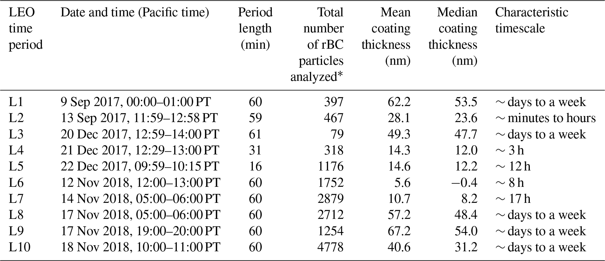
* LEO coating thickness calculations shown in the table only include rBC-containing particles with core sizes between 200 and 250 nm.
2.5 Time series filtering
rBC mass and number concentrations during the first campaign (September 2017) showed anomalous spikes likely due to unexpected local sources. In an effort to obtain representative background concentrations, we filtered these spikes by removing values above a threshold of 0.08 µg m−3 and 40 cm−3 for mass and number concentrations, respectively. Figure S2 shows the time series for the first campaign before and after removal of spikes. Figure S3 shows the median rBC concentration for the first campaign as a function of the cutoff threshold value. Median rBC mass and number concentrations approached asymptotic values at respective cutoff values of approximately 0.08 µg m−3 and 40 cm−3, suggesting that the median rBC concentration values become insensitive to the choice of cutoff threshold above these values.
2.6 Lag-time method
The mixing state of rBC was examined using two different methods. The first method used to characterize the mixing state is called the lag-time method. This method categorizes each rBC particle as either “thickly coated” or “thinly coated” based on a measured time delay (i.e., “lag time”) between the scattering and incandescence signal peaks. This method has been previously described and used in various studies (Moteki and Kondo, 2007; McMeeking et al., 2011a; Metcalf et al., 2012; Sedlacek et al., 2012; Wang et al., 2014; Krasowsky et al., 2016, 2018). In short, as a coated rBC-containing particle passes through the SP2 laser, the sensors will detect a scattering signal as the coating vaporizes. Shortly after, there will be a peak in the incandescence signal as the rBC core heats up and emits thermal radiation. A probability density function of the lag-time values often results in a bimodal distribution (Moteki and Kondo, 2007; McMeeking et al., 2011b). Based on the data for a particular campaign, a lag-time cutoff is chosen between the two peaks of the bimodal distribution to bin each rBC particle as either thinly or thickly coated. The fraction of rBC particles that are thickly coated (fBC) is then determined based on this categorization. For our study, a lag-time cutoff of 1.8 µs was chosen to quantify whether an rBC-containing particle was thickly coated or not. Only particles with an rBC core diameter greater than 170 nm were included in the calculation of fBC to account for the scattering detection limit of the instrument. As discussed previously by Krasowsky et al. (2018), the lag-time method is inherently susceptible to biases as fBC can depend on the selection of the lag-time cutoff value. For example, Krasowsky et al. (2018) selected a cutoff value of 1 µs for a near-highway SP2 campaign in the Los Angeles Basin, which is significantly different from the value of 1.8 µs used in this study and others. An unresolved issue remains with respect to maintaining consistency between different studies utilizing the lag-time method while simultaneously representing the unique mixing state characterization of each measured rBC population; the definition of “thickly coated” likely varies with the aerosol population sampled and, thus, is not necessarily comparable from one study to the next.
2.7 Leading-edge-only (LEO) method
The BC mixing state was also characterized using the LEO method. In brief, this method reconstructs a Gaussian scattering function from the leading edge of the scattering signal for each rBC-containing particle. The width and location of the reconstructed Gaussian scattering function are determined by a two-element avalanche photodiode. Assuming a core–shell morphology, the rBC coating thickness is subsequently calculated using Mie theory from the reconstructed scattering signal and the incandescence signal (Gao et al., 2007; Moteki and Kondo, 2008). Refractive indices of (2.26+1.26i) and (1.5+0i) were selected for rBC cores and rBC coating material, respectively. These parameters were selected based on recommendations and results from previous studies (Moteki et al., 2010; Dahlkötter et al., 2014; Taylor et al., 2014, 2015). The Paul Scherrer Institute's single-particle soot photometer toolkit version 4.100b (developed by Martin Gysel et al.) was used to perform the LEO method in Igor Pro version 7.09.
In this study, the LEO “fast-fit” method was used with three points, and particles analyzed were restricted to those with rBC core diameters between 180 and 300 nm. Although the SP2 has been reported to accurately measure the volume equivalent diameter (VED) of scattering particles down to ∼170 nm, a more conservative lower threshold of 180 nm was used for our study to reduce instrument noise at smaller VED values near the detection limit (Krasowsky et al., 2018). Specific rBC core diameter ranges were used for different analyses in this study, and these ranges are explicitly defined within each respective discussion. One exception was made to the 180–300 nm rBC core diameter restriction in Sect. 3.7. For the analyses and discussion presented in Sect. 3.7, the LEO coating thickness was calculated for all detectable rBC particles with non-saturated scattering signals. The rBC core size was not restricted in this section because the relative comparisons between characteristic coating thickness values were more important for the analysis, rather than the absolute value (which would likely be biased, as discussed further in Sect. 3.8). In other words, the LEO-derived coating thickness values in Sect. 3.7 were not used to report representative averages for selective time periods, but they were rather used for comparative and/or qualitative purposes.
Negative LEO-derived coating thickness values are reported throughout the results and discussion section. These nonphysical results are caused by instrument noise from both the incandescence and scattering detectors. The per-particle uncertainty associated with both of these signals results in a spread of coating thickness values that are at times less than zero. As a hypothetical example, a thinly coated particle that has its scattering cross section underestimated and its rBC mass equivalent diameter overestimated may result in a negative coating thickness value. According to Metcalf et al. (2012), the per-particle coating thickness uncertainty is ∼40 %, with the uncertainty reduced for larger rBC particles. In contrast to the per-particle uncertainty, systemic uncertainty, which is that associated with the average of the population of particles, is largely caused by the choice of the assumed parameters for the rBC core, namely its refractive index and density (Taylor et al., 2015). These systemic errors complicate direct comparison between measurements conducted with different sets of parameters assumed for the rBC core, but they do not affect comparisons within the same set of measurements. Negative LEO-derived coating thickness values have been reported in numerous past studies, and further details regarding both the per-particle and systemic uncertainties can be found in these studies (Metcalf et al., 2012; Laborde et al., 2013; Krasowsky et al., 2018; Taylor et al., 2015).
This section starts by discussing the major identifiable sources and meteorological patterns in each of the three campaigns (Sect. 3.1). Then, the overall mass and number loading of rBC are discussed and compared to past literature values (Sect. 3.2). Following that, the rBC mixing state results from the lag-time and LEO analyses are discussed (Sect. 3.3–3.5). The impacts of the emissions source type and atmospheric aging on the rBC mixing state and core size are subsequently discussed (Sect. 3.6 and 3.7). Section 3 then ends by comparing the rBC coating thickness values calculated in this study to reported values from past studies
3.1 Source identification and meteorology
In this section, we summarize the dominant pollutant sources and wind patterns for each of the three campaigns. For all three campaigns, we used HYSPLIT back-trajectories, HYSPLIT dispersion model, CAMS model data, and NASA data products (i.e., satellite imagery, aerosol index products, and AOD products) in conjunction to identify the most likely sources of measured rBC-containing particles. For the first campaign (September 2017), the Oregon wildfires were identified as probable sources of measured rBC. Furthermore, we also identified long-range transport from East Asia as well as ship and aviation emissions as potential sources contributing to measured rBC. Overall, we expect measured rBC during the first campaign to be aged. For the second campaign (December 2017), fresh urban emissions from the Los Angeles Basin and biomass burning emissions from the Thomas Fire in Santa Barbara and Ventura County (along with other smaller southern California fires) were the main sources identified by our analysis. For the third campaign (November 2018), fresh urban emissions from the Los Angeles Basin and fresh biomass burning emission from the Woolsey Fire in Ventura (along with other smaller southern California fires) were the main sources identified for approximately the first 4 d of the campaign. For the last 2 d of the third campaign, the Camp Fire in northern California (along with other smaller fires in northern and central California) contributed significantly to measured rBC. Figure 2 displays wind roses for each campaign at three different weather station locations (public data provided by NOAA; see Sect. 2.3). Moreover, Fig. 3 shows HYSPLIT back-trajectories simulated for each of the three campaigns and further highlights the differences in wind conditions between the three campaigns. These figures show the distinct meteorological regimes of each campaign. A more detailed description of the source identification process can be found in Sect. S2.

Figure 2Wind roses for the September 2017 (a, d, g), December 2017 (b, e, h), and November 2018 (c, f, i) sampling periods. Wind roses are based on 5 min Automated Surface Observing System (ASOS) airport data from LAX (a–c), LGB (d–f), and AVX (g–i), provided by NOAA.
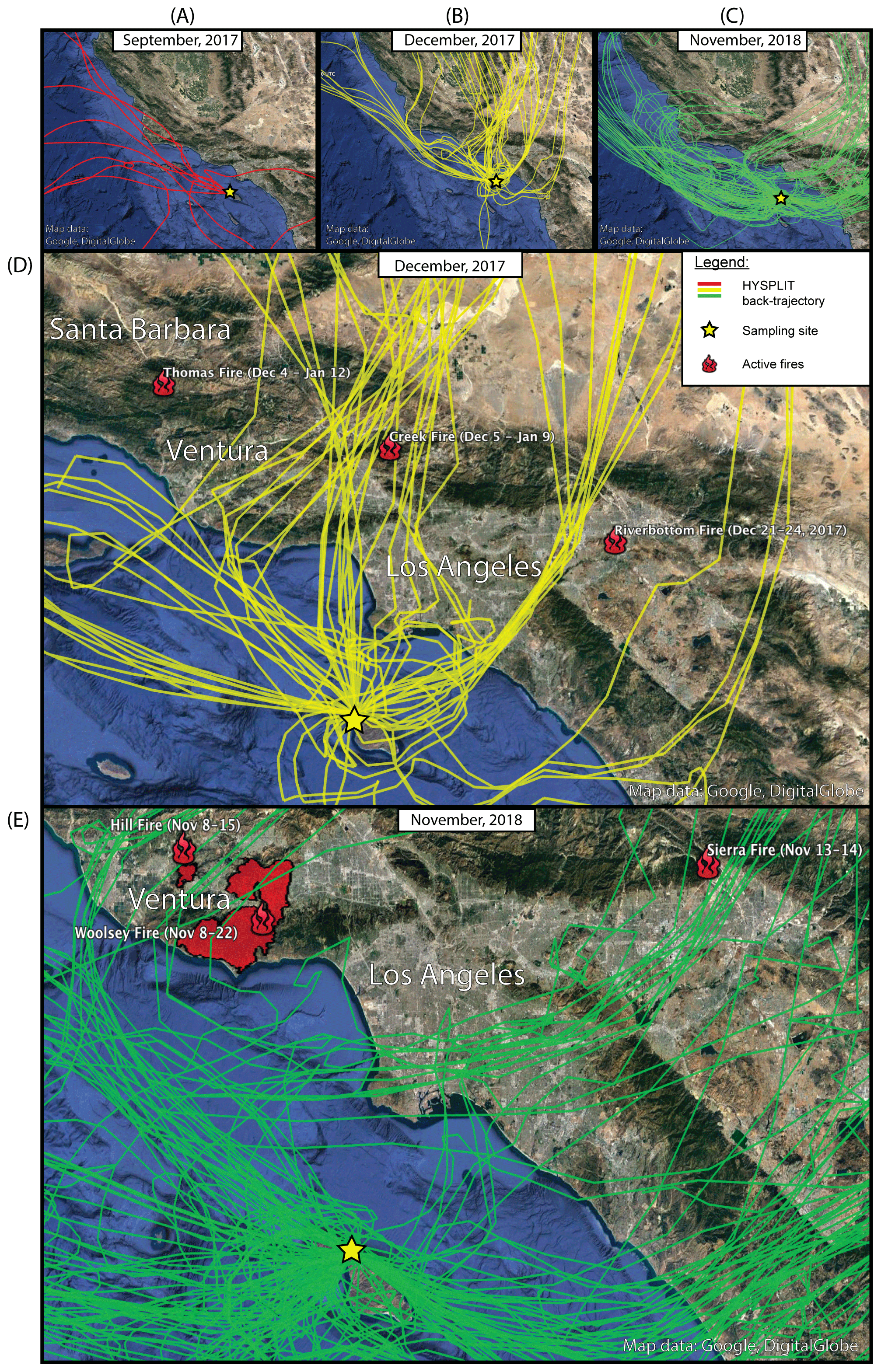
Figure 3HYSPLIT back-trajectories for all three campaigns. The star denotes the starting location of each back-trajectory, i.e., the sampling location. The trajectories for the first period (September 2017; a) represent week-long back-trajectories for each day of the campaign. The trajectories for the second (December 2017; b) and third (November 2018; c) periods represent 72 h back-trajectories for each hour of the campaign. Panels (d) and (e) show more zoomed-in maps of the respective second and third campaign back-trajectories along with active southern California fires. Map data © Google Earth.
For the remainder of the paper, we refer to rBC measured when the dominant source was biomass burning emissions as BCbb; rBC measured when the dominant source was fossil fuel (e.g., urban) emissions is referred to as BCff; and rBC measured in the first campaign (September 2017), when the measured air masses were representative of well-aged background over the Pacific Ocean, is referred to as BCaged,bg.
3.2 The rBC mass and number concentration
Figure 4 shows time series for the rBC mass and number concentrations, the rBC coating thickness (CTBC), the number fraction of thickly coated particles (fBC), and the rBC count mean diameter (CMD) for all three measurement campaigns. The mixing state (CTBC and fBC) and rBC size are discussed in following sections. The mean mass and number concentration (± SD – standard deviation) for the first campaign (September 2017) was 0.04 (±0.01) µg m−3 and 20 (±7) cm−3, respectively. For the second campaign (December 2017), the corresponding mean concentrations were 0.1 (±0.1) µg m−3 and 63 (±74) cm−3, with concentrations reaching as high as 0.6 µg m−3 and 381 cm−3. Likewise, for the third campaign (November 2018), the corresponding mean concentrations were 0.15 (±0.1) µg m−3 and 80.2 (±54.5) cm−3. The range of observed rBC concentrations is larger for the second and third campaigns compared with the first campaign, and there are distinct prolonged peaks in concentrations that can be observed during these times. In comparison, the first campaign shows relatively stable concentrations.

Figure 4Time series of (a) the BC absolute coating thickness, (b) the number fraction of thickly coated rBC particles, (c) the rBC count median diameter, and (d) the rBC concentrations, for all three measurements campaigns. The boxed annotations (i.e., L1 to L10) refer to specific LEO periods, which are further described in Sect. 3.5. In panel (a), each blue dot represents an individual particle. The hourly median is shown using the dotted pink line, and the corresponding 10th and 90th percentiles are shown in purple. In panel (b), green dots represent 1 min means, and the black curve shows hourly means. Panel (c) shows the 1 min mean for the count mean diameter. Panel (d) shows the 1 min means for rBC concentration. Dates on the x axis are given in the following format: month/day/year.
Given the remote location of the sampling site and the consistent westerly winds during the first campaign (September 2017), the observed rBC concentrations establish an appropriate baseline for ambient conditions away from the broader urban plume in the Los Angeles Basin. On the other hand, the concentrations during the second and third campaigns (December 2017 and November 2018, respectively) were more variable, with mean concentrations that were higher than the first campaign due to periods of northerly-to-easterly winds driven by Santa Ana wind conditions, as described in Sect. 3.1. Figure 5 shows the rBC mass and number concentrations along with wind speed and direction during the second campaign. The wind direction was directly related to elevated concentrations for all three peaks shown. Peak P1 is clearly preceded by a prolonged period of northerly winds. Similarly, peaks P2 and P3 are preceded by periods of easterly winds. An analogous plot for the third campaign is shown in Fig. S8, but the relationship between the wind direction measured at LAX and the rBC concentration is not clearly discernible because long-distance biomass emissions were impacting the measurements in addition to local sources near the LA Basin. The impacts of different sources on measurements during the third campaign are described in detail in Sect. S2.
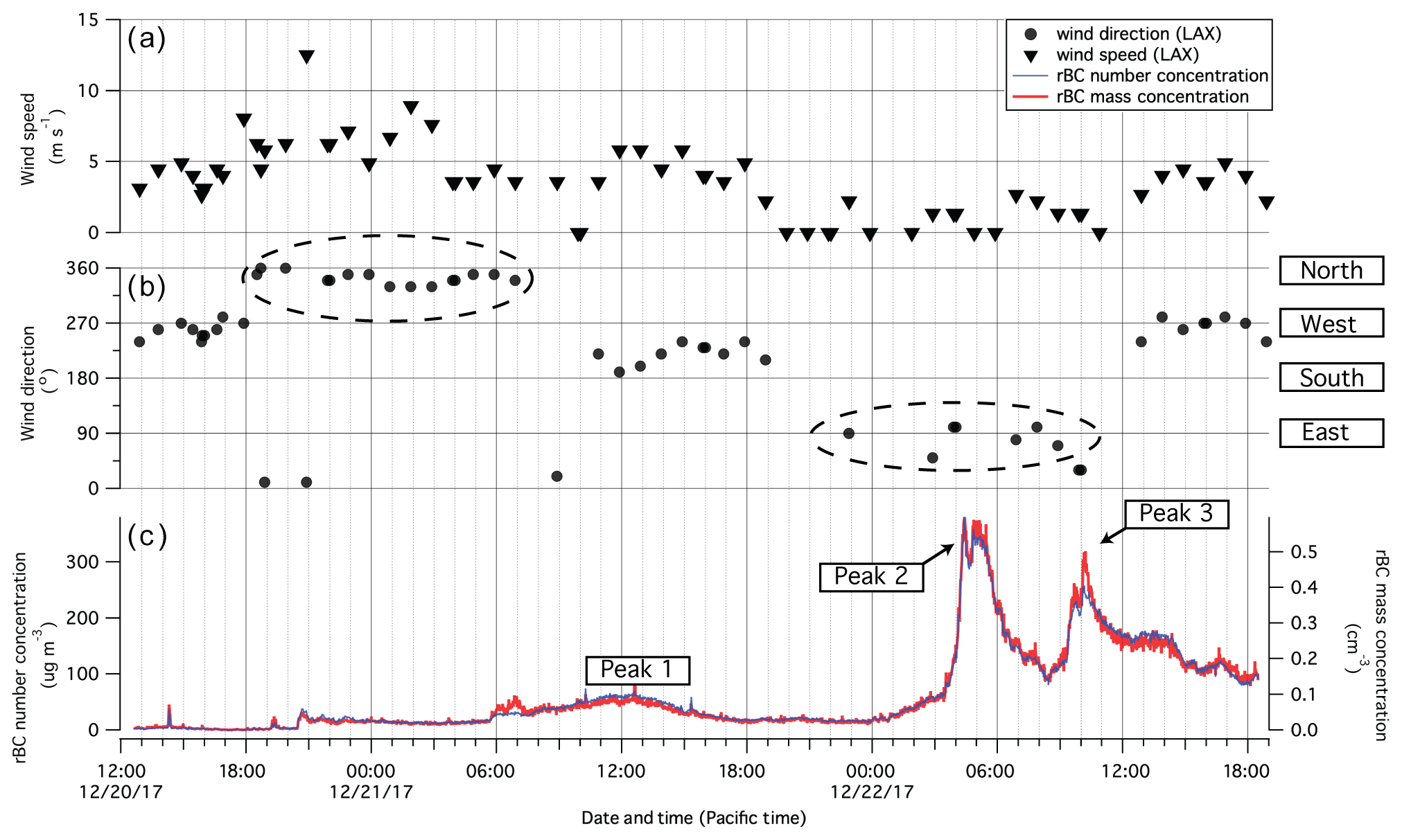
Figure 5Meteorological variables and rBC concentrations during the second campaign (December 2017). Panel (a) shows wind speed and panel (b) shows the wind direction measured by a NOAA weather station located at Los Angeles International Airport (LAX). Panel (c) shows the rBC mass and number concentrations and identifies three peaks of interest. The two dashed ovals in panel (b) highlight periods of northerly and easterly winds, which occur ∼0.5–1 d before each of the three peaks, suggesting that the elevated rBC concentrations included important contributions from the local Thomas Fire (and other smaller fires) and urban emissions from the Los Angeles Basin. Dates on the x axis are given in the following format: month/day/year.
The mean concentration for the first campaign (September 2017) was approximately an order of magnitude lower than the mean concentration of ∼0.14 µg m−3 observed by Krasowsky et al. (2018) near the downwind edge (assuming dominant westerly wind flows) of the LA Basin (i.e., Redlands, California). Concentrations during the most polluted time periods in our measurements were comparable to recently measured concentrations in the Los Angeles Basin (Krasowsky et al., 2018) but were at least 1 to 2 orders of magnitude lower than average concentrations found in other heavily polluted cities around the world. Mass concentration values of ∼0.9, ∼0.5 to 2.5, ∼0.9 to 1.74, and ∼0.6 µg m−3 were measured with an SP2 in Paris, Mexico City, London, and Houston, respectively (Laborde et al., 2013; Baumgardner et al., 2007; Liu et al., 2014; Schwarz et al., 2008a). In urban areas of China, an average mass concentration of ∼9.9 µg m−3 was reported for a polluted period in Xi'an (Wang et al., 2014).
3.3 Lag-time analysis: the number fraction of thickly coated rBC-containing particles
Figure 4b shows both 1 min and 1 h means for fBC over the course of all three campaigns. On average, fBC was larger during the first campaign (September 2017) than during the second and third campaigns (December 2017 and November 2018, respectively). The mean values (± SD – standard deviation) of fBC were 0.27 (±0.19), 0.03 (±0.09), and 0.14 (±0.15) for the first, second, and third campaigns, respectively. This implies that about one-quarter of the rBC-containing particles that were measured in the first campaign either had sufficient time in the atmosphere to become aged with thick coatings or originated from biomass burning emission sources, which have been shown to emit more thickly coated particles compared with fossil fuel emissions (Dahlkötter et al., 2014; Laborde et al., 2013; Schwarz et al., 2008a). Most of the rBC particles measured in the second campaign were thinly coated, implying that BCff dominated measurements. The rBC from the third campaign exhibited mostly thinly coated rBC for the first ∼4 d of the campaign and an increased fBC for the last ∼2 d of the campaign.
Compared to past studies in the Los Angeles region, the mean fBC for the first campaign (September 2017) (fBC=0.27) is close to the lower end of values from aircraft measurements (fBC=0.29) (Metcalf et al., 2012) and the upper end of previous ground-based measurements (fBC=0.21) (Krasowsky et al., 2016). In contrast, the mean value of fBC for the second campaign (December 2017) is almost an order of magnitude lower than that from the first campaign. There are some periods with slightly elevated fBC during the second campaign, but the overall trend suggests that most of the rBC-containing particles in this period are thinly coated or essentially uncoated. The Santa Ana wind conditions during the second campaign advected fresh (a) urban emissions from the Los Angeles Basin and (b) biomass burning emissions from active fires in southern California, as discussed in Sect. 3.1.
The third campaign (November 2018) is unique in that both “fresh” and “aged” BCbb as well as fresh BCff were measured. As shown in Fig. 4, there is a distinct period of relatively higher fBC and rBC concentrations starting at roughly noon on 16 November 2018 and lasting through the end of the campaign on 18 November 2018. This is the only period from all three measurement campaigns where we observed both high rBC mass and rBC number loadings as well as high fBC values. In Sect. 3.1, we identified the Camp Fire to be the dominant source during this time period within the third campaign. Thus, the biomass burning rBC particles measured in this portion of the third campaign are more thickly coated than our measured urban rBC. Previous field studies have reported that BCff generally has a lower fBC relative to BCbb (Schwarz et al., 2008a; Sahu et al., 2012; Laborde et al., 2013; McMeeking et al., 2011b; Akagi et al., 2012). For example, Schwarz et al. (2008a) reported an fBC∼10 % for urban emissions and an fBC∼70 % for biomass burning emissions. The impact of source type on the rBC mixing state will be further discussed in Sect. 3.7.
3.4 Negative lag times and rBC morphology
A number of previous studies (Moteki and Kondo, 2007; Sedlacek et al., 2012, 2015; Moteki et al., 2014; Dahlkötter et al., 2014) have reported negative lag times from both laboratory and field measurements of rBC. It has been hypothesized that a negative lag time is observed when rBC fragments from its coating material, resulting in a scattering signal that follows an incandescent signal. Dahlkötter et al. (2014) summarized that negative lag times can occur when (i) rBC is very thickly coated in a core–shell configuration, (ii) rBC is thickly coated and the core is offset from the center in an eccentric arrangement, or (iii) rBC is located on or near the surface of an rBC-free particle. The morphology of rBC-containing particles is of importance because the enhancement of BC light absorption can vary widely depending on whether the morphology more closely resembles a core–shell configuration or near-surface attachment (Moteki et al., 2014). Although the fraction of negative lag times (flag,neg) cannot definitively identify the morphology of individual rBC-containing particles (Sedlacek et al., 2015) or accurately quantify the actual percentage of all fragmenting rBC-containing particles (Dahlkötter et al., 2014), it can offer some general insights about rBC morphology, especially when it is paired with other information like the emission source type and rBC coating thickness. flag,neg is a conservative lower-bound estimate for the fragmentation rate because there may be rBC particles with positive lag times that still fragment in the SP2 (Dahlkötter et al., 2014). Dahlkötter et al. (2014) used a method examining the tail end of the time-dependent scattering cross section in order to determine if a rBC-containing particle was fragmenting, thereby calculating a higher fragmentation rate relative to flag,neg. Details of the time-dependent scattering cross-section method can be found in Laborde et al. (2012) and Dahlkötter et al. (2014). This method to calculate a refined fragmentation rate was not used in Sedlacek et al. (2012) nor in this study.
Furthermore, Sedlacek et al. (2012, 2015) suggest that flag,neg and the lag-time distributions may assist in source attribution. More specifically, Sedlacek et al. (2012) measured a confirmed biomass burning plume in August 2011 and found a high positive correlation between biomass burning tracers and flag,neg during the period of impact, suggesting that flag,neg may be a useful indicator of biomass burning influence.
In this study, we observed negative lag times, although at a relatively low rate, with flag,neg calculated to be much less than 0.1 throughout most of the measurement periods (see Fig. 6). We defined flag,neg to be identical to the “fraction of near-surface rBC particles” metric used by Sedlacek et al. (2012), using a lag-time threshold of −1.25 µs to account for uncertainties associated with the lag-time determination. The campaign-wide flag,neg was 0.017 for the first campaign (September 2017), 0.018 for the second campaign (December 2017), and 0.026 for the third campaign (November 2018). Comparatively, Dahlkötter et al. (2014) observed an flag,neg of ∼0.046 during an airborne field campaign measuring an aged biomass burning plume, and additionally calculated a higher fragmentation rate of ∼0.4 to 0.5, based on their aforementioned alternative method (Laborde et al., 2012). Sedlacek et al. (2012) reported an for ground-based measurements of a biomass burning plume in Long Island, New York, originating from Lake Winnipeg, Canada.

Figure 6Panel (a) shows the 10 min mean time series for the number fraction of rBC particles with negative lag times (flag,neg). The threshold for negative lag times was set to −1.25 µs to account for uncertainties in the lag-time determination (Sedlacek et al., 2012). Panel (b) shows the time series of lag-time values for each individual particle, corresponding to individual dots on the graph. Panel (c) shows the 1 min mean rBC number concentration for reference. Dates on the x axis are given in the following format: month/day/year.
The widely varying flag,neg between these different studies (including our study) suggests that flag,neg may not be a useful metric when comparing between studies. One of the key findings from Sedlacek et al. (2015) shows that SP2 operating conditions strongly affect the frequency of negative lag times and suggests that inter-study comparisons of flag,neg could be meaningless, or at worst misleading, if the laser power and sample flow rate are not reported. See Sect. S3 for more details.
The higher mean value of flag,neg (0.026) during the third campaign (November 2018), relative to the first (0.017) and second (0.018) campaigns, shows that flag,neg could potentially be a useful as a supplemental metric when identifying impacts from biomass burning sources, as mentioned by Sedlacek et al. (2012, 2015). Figure 7 also shows that the 10 min mean negative lag times increase in magnitude with increasing rBC core diameter between the range of ∼100 and 115 nm (i.e., higher rates of fragmentation with increasing core size). This follows a similar trend to that observed by Sedlacek et al. (2012, 2015), who attributed this trend to increased heat dissipation to surrounding gases for smaller rBC cores, which in turn decreases the particle heating rate and, consequently, decreases the fragmentation rate. Our observations add to the limited past observations that show that the fragmentation rate of rBC particles in the SP2 depends on physical factors like the core size. This further complicates the practical use of flag,neg as a biomass burning indicator.
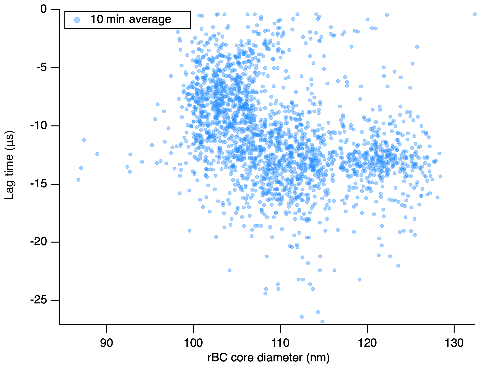
Figure 7Scatterplot of 10 min mean negative lag times versus 10 min mean rBC core diameters.
Certain trends in flag,neg for this study further indicate that it should not be used in isolation to verify the relative abundance of biomass burning aerosol versus non-biomass burning aerosols. There are peaks in the flag,neg time series (Fig. 6) that do not follow the expected trends based on identifiable source impact time periods. For example, the two peaks on 22 December 2017 (BCff periods) correspond to flag,neg values exceeding 0.02, but flag,neg hovers around 0.02 on 17 November 2018, when we had expected direct impact from the Camp Fire. As evidenced from the meteorology (Sect. 3.1), mixing state (Sect. 3.3), rBC concentrations (Sect. 3.2), and rBC core size (to be discussed in Sect. 3.6), measurements on 17 November 2018 were dominated by biomass burning emissions, but flag,neg fails to show that independently. These anomalous observations show that flag,neg needs to be used with caution and that future studies are necessary to extensively quantify the relationship between flag,neg and source type.
The observations of negative lag times in this study confirm that ambient rBC likely do not adhere strictly to core–shell morphology. The exact morphology of measured rBC cannot be quantified based on our measurements, but the presence of negative lag times in this study highlights the need to further understand rBC morphology and its effect on absorption enhancement in future studies as well as the potential for flag,neg to be used as a supplemental source identification tool.
3.5 Leading-edge-only (LEO) fit analysis: the rBC coating thickness
To further examine the mixing state of rBC-containing particles, the leading-edge-only (LEO) fit method was used to quantify rBC coating thickness (CTBC) on a particle-by-particle basis. Figure 4a shows the time series of CTBC throughout all three campaigns. The time series of CTBC shows that each campaign was characterized by different mixing states and that there are distinct trends within each campaign.
The inter-campaign differences are highlighted in Fig. 8, which shows the CTBC distribution for each campaign as well as the distribution including rBC from all campaigns. For both rBC core diameter ranges (180–220 and 240–280 nm), we observe that the first campaign has the largest mean CTBC, followed by the third and second campaign, respectively. The mean CTBC (± standard deviation) for the first, second, and third campaign was 52.5 (±45.5), 22.3 (±25.0), and 40.3 (±41.5) nm, respectively, for particles with a rBC core diameter between 180 and 220 nm.
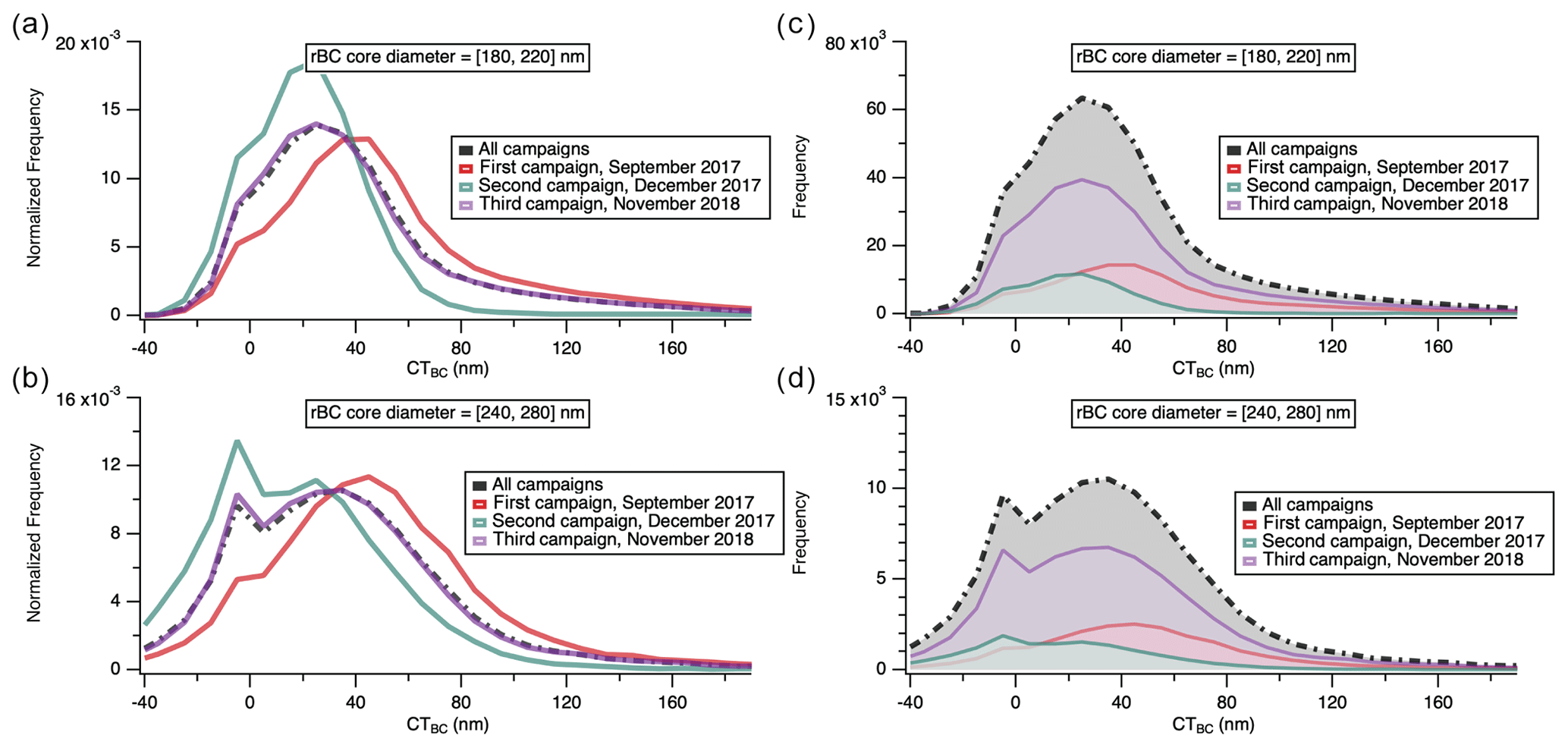
Figure 8Distributions of BC coating thickness (CTBC) aggregated by campaign are shown in red (first campaign), green (second campaign), and purple (third campaign). The combined distributions for all campaigns are shown in black. Panels (a) and (b) show the normalized frequency distributions, and panels (c) and (d) show the absolute frequency distributions. The distributions are also distinguished by the rBC core diameter ranges included in the LEO analysis. Panels (a) and (c) show distributions for particles with rBC core diameters between 180 and 220 nm; panels (b) and (d) show distributions for particles with rBC core diameters between 240 and 280 nm.
Comparing the time series of CTBC to the time series of fBC (Fig. 4), we observe similar trends over time, which is expected and has also been reported in past studies that have employed both the lag-time and LEO methods (Metcalf et al., 2012; Laborde et al., 2012; McMeeking et al., 2011a). Figure 9 shows a positive correlation between 10 min mean CTBC and fBC (r=0.82, r2=0.67) throughout all three campaigns. This strong correlation confirms that these two methods are in general agreement and that they can be used together to robustly describe the rBC mixing state.

Figure 9Scatterplot as a function of lag time (i.e., delay time) and BC coating thickness (CTBC). Each point on the plot represents a 10 min mean value. Data shown include average values from all three campaigns. A significant correlation is confirmed using a linear correlation test. The coefficient values a and b represent the y intercept and slope of the least squares fit, respectively.
In addition to aggregating CTBC by campaign, we also examined 10 discrete time periods of interest to obtain a more detailed understanding of the mixing state variability. Particles with rBC diameters between 200 and 250 nm were used in the comparison of these 10 time periods. Two time periods from the September campaign, three time periods from the December campaign, and five time periods from the November campaign were selected to represent a diverse range of meteorological conditions, emission sources, and the age of aerosols. Table 2 lists the 10 LEO-fit periods as well as their median and mean CTBC. The LEO-fit periods are also annotated on the rBC concentration time series (see Fig. 4) to show when they occurred in the context of all three campaigns. The median CTBC for the LEO periods ranged from −0.4 to 54.0 nm. L6 had the lowest median CTBC (−0.4 nm), whereas L9 had the highest median CTBC (54.0 nm).
Figure 10 illustrates the CTBC distributions and statistics of each LEO period. L1 and L2 were from the first campaign (September 2017). L1 is representative of ambient background rBC-containing particles from the first campaign. A period that did not exhibit any anomalously large rBC mass concentration values was chosen so that contributions from possible nearby sources would not skew the mean CTBC. Conversely, L2 intentionally spans a period with many anomalously high rBC mass concentration values. Although these anomalous values were removed from the concentration time series discussed previously in Sect. 2.4, the values were not removed for the LEO analysis of L2 in order to examine the relationship between CTBC and possible nearby emissions. As hypothesized, the rBC-containing particles from L2 were generally more thinly coated than those from L1. The median CTBC from L2 was ∼30 nm lower than that for L1, which corroborates our hypothesis that the anomalously high mass concentration values in the first campaign included contributions from nearby, unidentified fossil fuel sources.
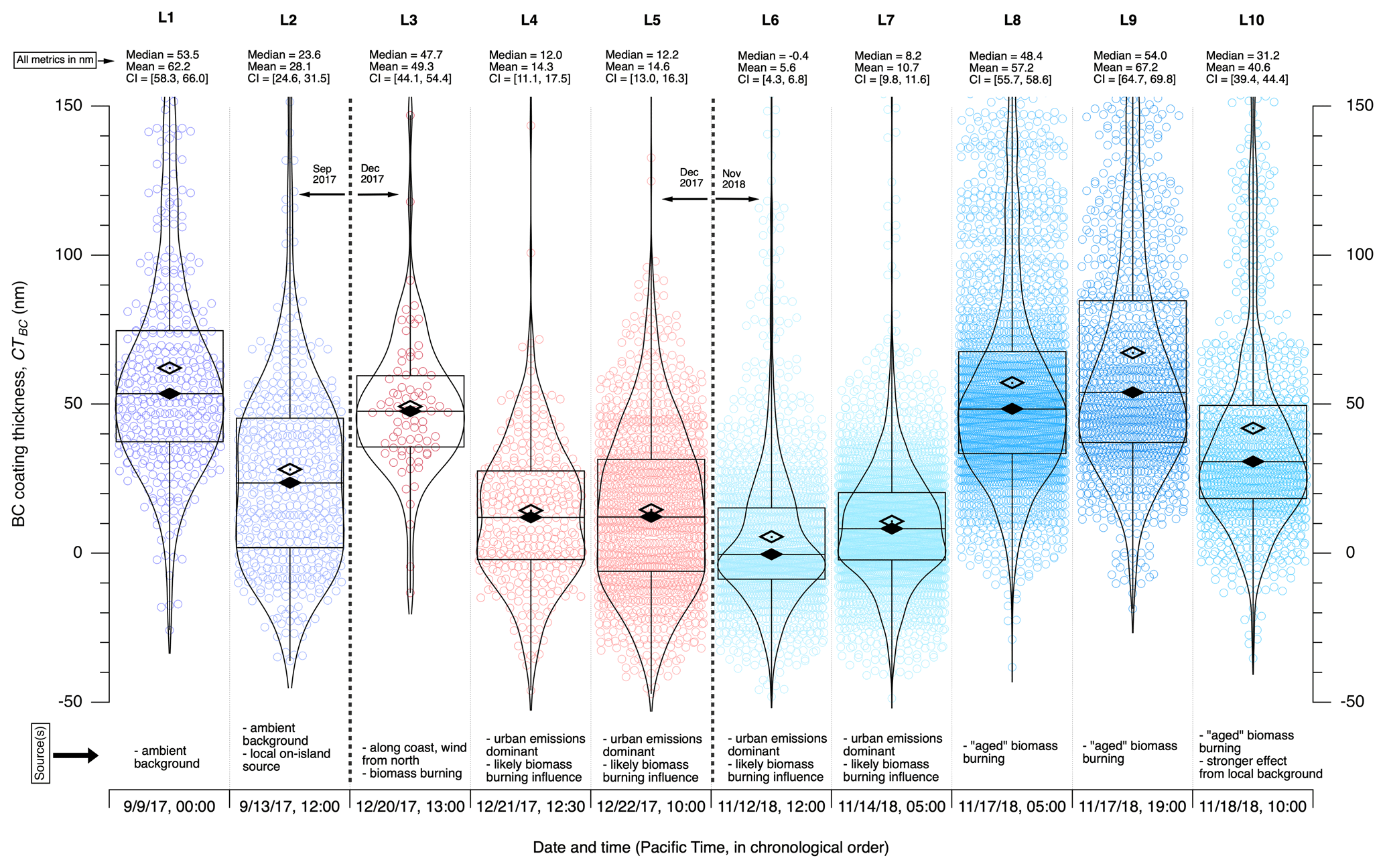
Figure 10Violin plots that show the distribution of rBC coating thickness values for particles with rBC diameters between 200 and 250 nm, calculated for each LEO time period, L1 through L10. Each circle marker in the plot represents a particle analyzed by the LEO analysis and the curves for each “violin” shape represent the normalized probability density function of the coating thickness for each LEO period. The violin shape results from mirroring each probability density distribution along a vertical axis. Box-and-whiskers plots are also overlaid to show the quartiles (25th, 50th, and 75th percentiles) of the coating thickness distributions. The 95 % confidence intervals (CI) based on a Student's t distribution are shown above each violin plot to demonstrate when the mean coating thickness values are statistically distinguishable from one another. The mean (unfilled diamond) and median (solid diamond) coating thicknesses are also indicated above each violin plot, and a brief description of sources for each LEO period is annotated below each distribution. Dates on the x axis are given in the following format: month/day/year.
L3 through L5 are time periods from the second campaign (December 2017). L3 represents a period near the start of the second campaign (December 2017). The predominant wind direction during L3 was westerly, with a mean wind speed of ∼4.5 m s−1. HYSPLIT back-trajectories and CAMS data show that L3 likely included important contributions from the Thomas Fire in Santa Barbara and Ventura County. The PM2.5 concentration gradient from CAMS was examined over time to track the movement of plumes that influenced the measurements during this time period. A few days prior to the start of the second campaign, the Thomas Fire resulted in a large aerosol plume westward over the Pacific Ocean. From visually tracking PM2.5 concentration gradients, it appears that a large-scale, clockwise, atmospheric circulation brought aerosols from the Thomas Fire to Catalina Island around the time of L3 (see Video 2 in the Video Supplement). The average concentration during L3 was about an order of magnitude lower than the average concentration for the September campaign. This could be partially attributed to the fact that L3 was around 13:00 to 14:00 PT, when the planetary boundary layer would be expected to increase in height, causing pollutant concentrations to decrease due to dilution. The median CTBC for L3 was 47.7 nm, which is slightly lower than for L1, which is representative of the ambient background conditions. The slightly smaller CTBC for L3 likely reflects the fact that the mixing state is sensitive to the source of emissions. In this time period, urban emissions were likely mixed into the regional air mass, slightly lowering the median CTBC. In this case, we have evidence to support that a larger fraction of measured rBC during L3 came from the local Thomas Fire mixed with nearby urban emissions, whereas L1 represents a mix of influences, including, but not limited to, aged biomass burning aerosols. The effect of the emissions source type on the rBC mixing state is discussed in Sect. 3.7.
L4 through L7 represent periods when the Los Angeles Basin, Santa Barbara and Ventura counties, and San Diego county (to a lesser degree) were identified as major sources. Air masses measured during these periods likely contained a mixture of both urban emissions and biomass burning emissions (see Sect. S2 and the accompanying figures), although urban emissions were likely dominant. Overall, these LEO periods exhibit the lowest median CTBC, ranging from −0.4 to 12.2 nm. The potential relationship between aging time and CTBC is discussed further in Sect. 3.7.
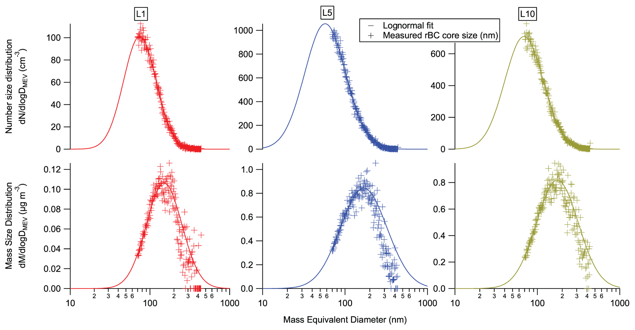
Figure 11rBC core size distributions and corresponding lognormal fits for LEO periods L1, L5, and L10.
L8 through L10 are the unique LEO periods from the third campaign (November 2018) with concurrently increased rBC concentrations and fBC (discussed in the previous section). We also observed significantly higher CTBC values during these periods compared with L4 through L7, with median CTBC ranging from 31.2 to 54.0 nm. We have strong evidence to support that the sampled particles include important contributions from aged rBC from the northern California fires, particularly the Camp Fire (see Sect. S2). The relatively high CTBC values in L8 and L9 (compared with other LEO periods) further support our claim that rBC-containing particles from northern California fires were dominating our measurements during this time. L10 has a median CTBC of 31.2 nm, which is ∼23 nm lower than the median value for L9. This reduction in the median CTBC is also reflected in the decrease of the fBC values near the end of the campaign. Meteorological data, MODIS satellite images, and CAMS data during this time period suggest that sources from the southern California (and possibly Central Valley) region contributed more to measurements during L10 than they did during L8 and L9, explaining the lower CTBC and higher overall concentrations. Wind speeds were lower on average for L10 compared with L8 and L9. The mean wind speed for L10 at LAX, based on 5 min NOAA data, was ∼1.3 m s−1, whereas the mean wind speeds for L8 and L9 were ∼2.1 m s−1 and 1.6 m s−1, respectively. There was also a general shift in the wind direction from westerly to northeasterly, approximately half a day before L10 (see Fig. S8). MODIS satellite imagery and CAMS data also confirm that local to regional sources were likely impacting the measurements more during this period (see videos 3 and 4 in the Video Supplement), compared with L8 and L9. The meteorology, in addition to local to regional sources of emissions from the Los Angeles Basin and southern California, likely explain the reduction in CTBC and the near doubling of the rBC concentration level.
3.6 The rBC core size
The number- and mass-based size distributions for rBC cores were assessed for periods L1 to L10. Similar to past studies, rBC core mass equivalent diameters between 70 and 450 nm are reported (Gao et al., 2007; Moteki and Kondo, 2007; Dahlkötter et al., 2014; Krasowsky et al., 2018). Figure 11 shows the rBC core size distributions and the corresponding lognormal fits for three LEO periods (L1, L5, and L10); we investigated these three LEO periods to assess whether lognormal fits adequately represent the actual rBC size distributions before presenting lognormal fits for all LEO periods. Previous studies have shown that rBC core size distributions are generally lognormal in the accumulation mode (Metcalf et al., 2012). Figure 11 shows that lognormal fits adequately capture the measured size distributions, although we cannot rule out the possibility of another rBC mode outside the detection limits of the SP2. Each of the 10 LEO periods were characterized by a single mode within the range of the SP2 detection range. Although the peak of the measured number size distribution is not always discernible (e.g., L5 in Fig. 11), the conclusions made in the following analysis of rBC core size are unaffected by the uncertainty in the actual count median diameter. In addition, even in cases of ambiguous number size distribution peaks, we found that the right-hand side edge of the measured distribution was fit well by the lognormal distribution. Even if the distribution below the detection limit of ∼70 nm deviated from the assumed lognormal fit, the median diameter is unlikely to be sufficiently affected to substantively change any of the following conclusions made in this section.
A survey of past studies that have reported the lognormal fit rBC mass median diameter (MMDfit) and count median diameter (CMDfit) shows that the source of emissions has a strong influence on rBC core diameter (Cheng et al., 2018). The MMDfit (CMDfit) for BCbb, which has been reported to range from ∼130 to 210 nm (100 to 140 nm), is generally larger than the MMDfit (CMDfit) for BCff, which has been reported to range from ∼100 to 178 nm (38 to 80 nm) (Shiraiwa et al., 2007; Schwarz et al., 2008a; McMeeking et al., 2010; Kondo et al., 2011; Sahu et al., 2012; Metcalf et al., 2012; Cappa et al., 2012; Laborde et al., 2013; Liu et al., 2014; Taylor et al., 2014; Krasowsky et al., 2018). The MMDfit (CMDfit) for well-aged background BC was reported to range from ∼180 to 225 nm (90 to 120 nm) (Shiraiwa et al., 2008; Liu et al., 2010; McMeeking et al., 2010; Schwarz et al., 2010).
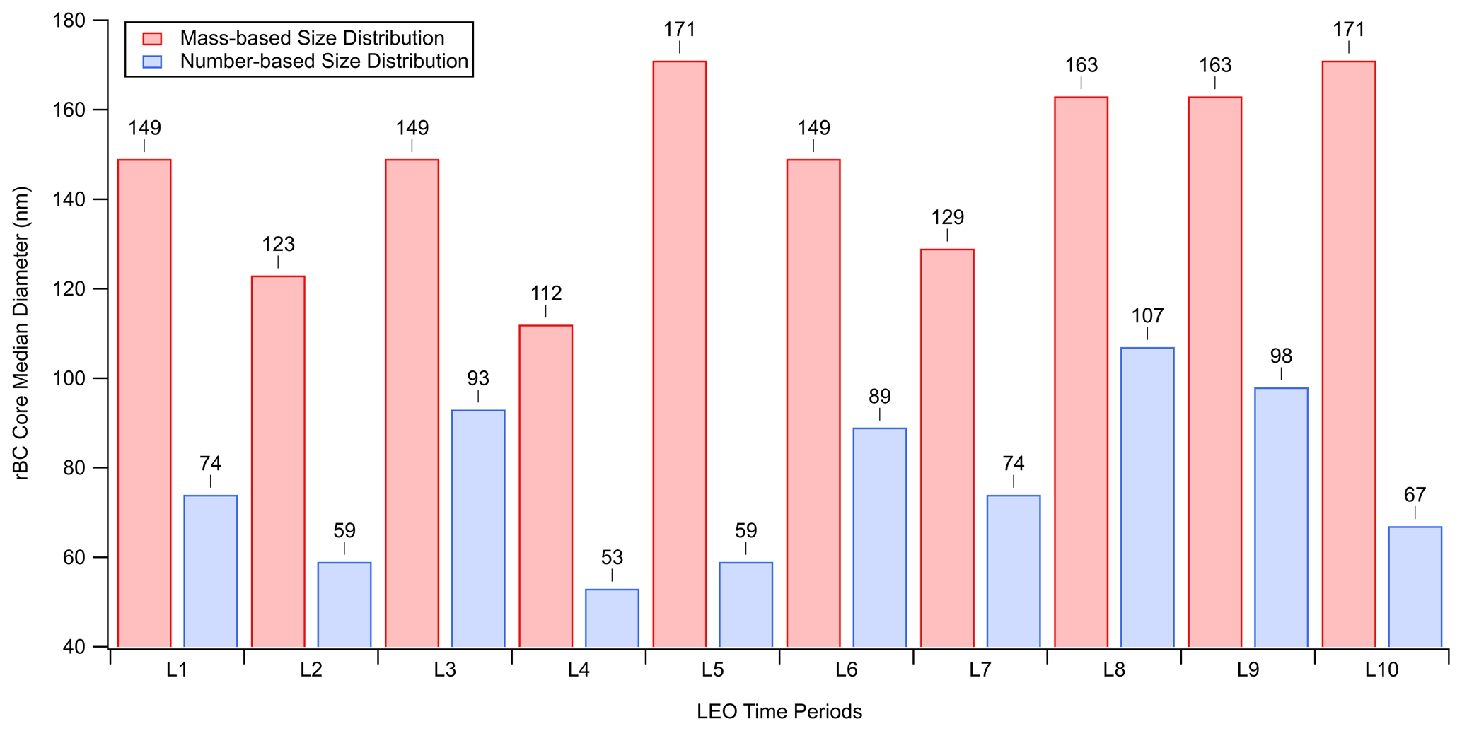
Figure 12Median rBC core diameter for both the mass and number size distribution lognormal fits.
Figure 12 shows the rBC MMDfit and CMDfit for each LEO period in this study. Based on the source identification discussed in Sects. 3.1 and S2, the MMDfit and CMDfit values in this study are generally consistent with the ranges reported in past studies. For BCbb (L3, L8, L9, and L10), MMD ranged from 149 to 171 nm, which is within the range of ∼130 to 210 nm reported in past studies. For BCff (L2, L4, and L7), the MMDfit dropped, ranging from 112 to 129 nm. This falls within the range of ∼100 to 178 nm previously reported for measurements of urban emissions.
Past literature has also mentioned the possibility of coagulation affecting the rBC core size (Bond et al., 2013). Shiraiwa et al. (2008) observed an increase in rBC core diameters in aged plumes compared with fresher urban plumes in the East Asian outflow, suggesting that coagulation can alter the rBC size distribution during atmospheric transport (i.e., aging). Although the emissions source type appears to be the dominant influence on rBC core sizes in our study, we cannot completely eliminate the possibility of any coagulation occurring between the point of emission and point of measurement. Our measurements suggest that coagulation would have a negligible impact at the measured number concentrations, but the number concentrations would be orders of magnitude higher near points of emission (especially in dense biomass burning plumes), leaving open the possibility of non-negligible coagulation near sources, in certain cases.
3.7 Impact of the emissions source type and aging on the rBC mixing state
The dominant factor that influences rBC core size (i.e., emission source type) also strongly influences the rBC mixing state. Figure 13 shows a scatterplot of 1 min mean CTBC versus 1 min mean rBC core diameter, using data from all three campaigns. A positive correlation was found, with r=0.55 and r2=0.30. This correlation suggests that larger contributions from biomass burning (as opposed to fossil fuel) are associated with increases in both the rBC core size and the BC coating thickness. Figure S22 shows the CTBC distributions for different rBC core size ranges, and a similar relationship between the two variables can be observed. As the core size increases (lighter to darker curves), a broader right-hand side tail is observed in the CTBC normalized distributions for each campaign, implying an increased probability density for thicker coatings as the rBC diameter increases.
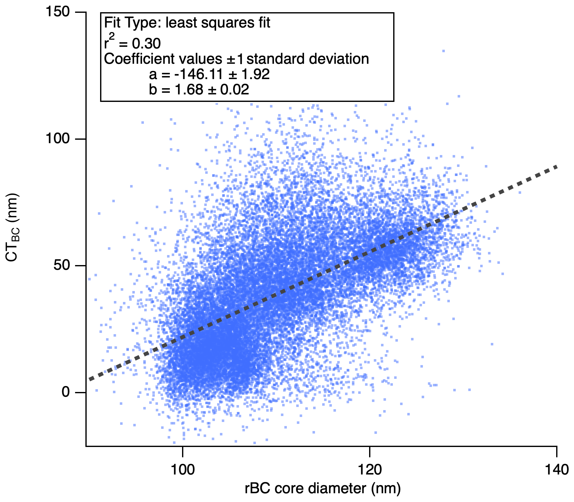
Figure 13The rBC coating thickness versus the rBC core diameter. Each point on the plot represents a 1 min mean. Data from all three campaigns are shown. CTBC values are calculated for particles with rBC core diameters between 200 and 250 nm. The line represents the least squares linear regression to the 1 min mean data points. There is a statistically significant positive correlation shown between CTBC and the rBC core diameter, as shown in the summary box in the top left corner. The coefficient values a and b represent the y intercept and slope of the least squares fit, respectively.
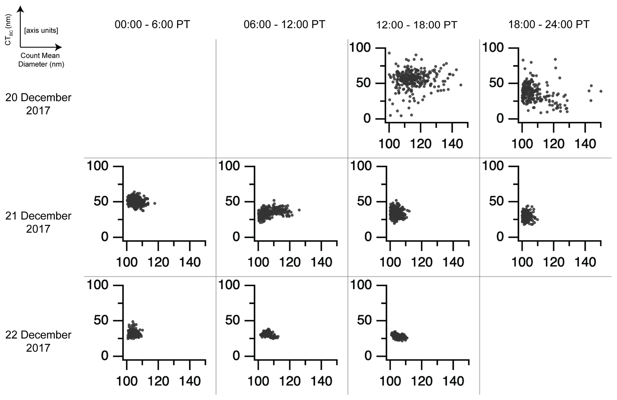
Figure 14Matrix of scatterplots showing the time evolution of CTBC (nm) and the rBC count mean diameter (nm) for the second campaign (December 2017). Axes labels are shown in the upper left. A scatterplot is shown for each 6 h time interval of the day, starting at 00:00 PT, and for each day of the campaign. The columns of the matrix denote the time interval of the day, and the rows of the matrix denote the days of the campaign. Each point within a plot represents a 1 min mean value for both CTBC and the count mean diameter.
The time evolution of both CTBC and the rBC core size is represented in a series of scatterplots in Figs. 14 and 15. In each of the figures, the scatter between the 1 min mean CTBC and rBC CMD are grouped into 6 h time intervals for both the second (December 2017) and third (November 2018) periods, respectively. In these figures, the time evolution of the rBC physical properties can be examined in detail and compared to periods of known emissions source impacts. There are a few significant patterns worth highlighting here. First, the influence of BCbb can be observed between 16 and 18 November 2018 in Fig. 15. Both CTBC and CMD drastically increase for a prolonged period of time, implying an impact from the Camp Fire plume from northern California. Second, the scatterplots for 20 to 22 December 2017 and from 12 to 15 November 2018 show that there is some variability over time in the cluster shapes, which can be explained by the local wildfires that were confirmed to have influenced the broader LA Basin plume (see Sect. S2 for details regarding source attribution). Although the scatterplots during these time periods support that BCff was largely dominant, there are some periods where the CMD spread deviates quite noticeably (e.g., Fig. 14, 06:00 PT on 21 December 2017), or even periods that show two distinct clusters (e.g., Fig. 15, 12:00 PT on 12 November 2018), supporting our claim that local wildfires in southern California were indeed influencing our measurements. A similar figure for the first campaign (September 2017) is included in Fig. S23, but it is not shown here because of the relatively stable mixing state and size of BCaged,bg. These figures confirm the general patterns noted in previous sections regarding the effects of different sources on the rBC mixing state.
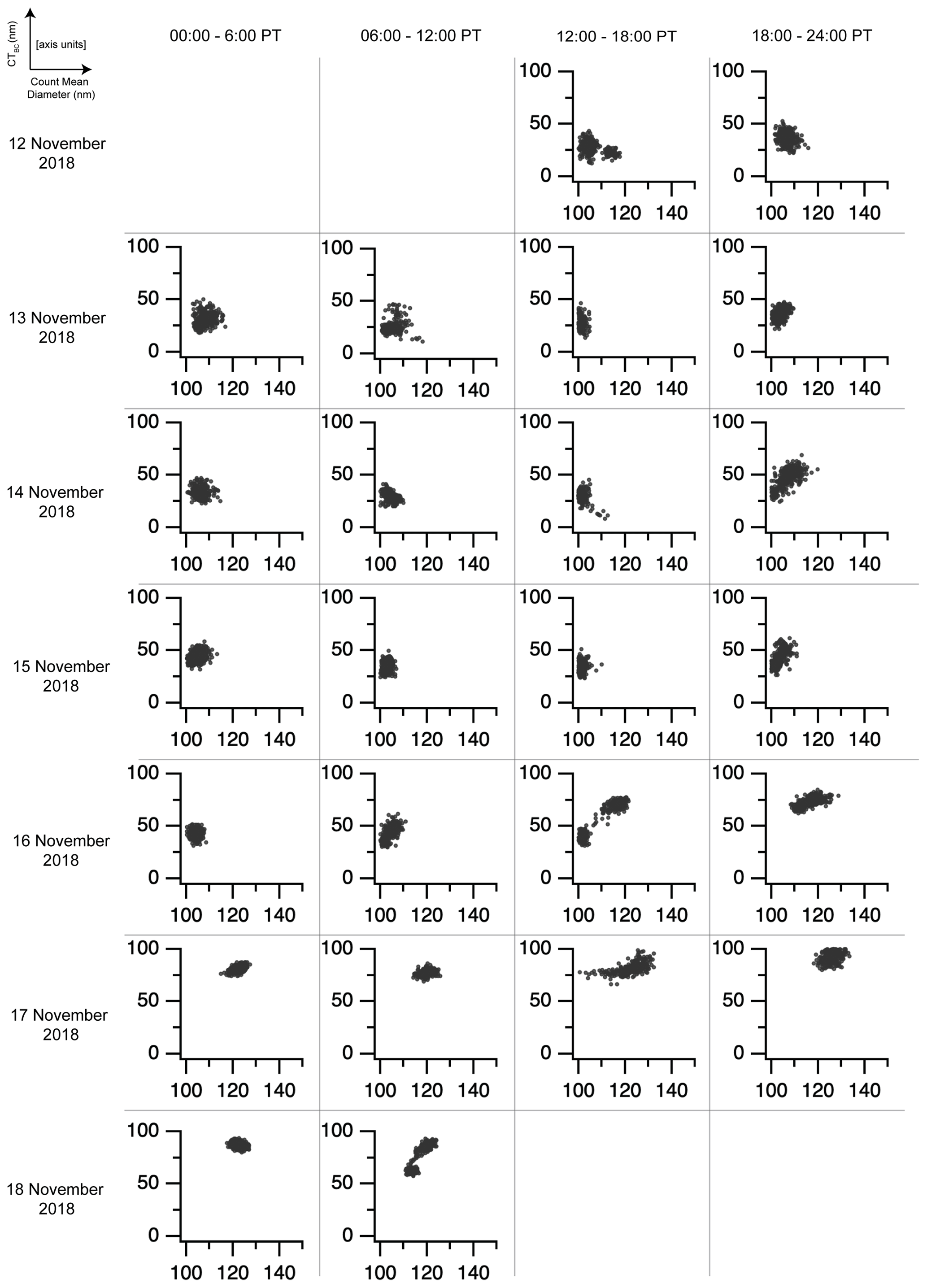
Figure 15Matrix of scatterplots showing the time evolution of CTBC (nm) and the rBC count mean diameter (nm) for the third campaign (November 2018). Axes labels are shown in the upper left. A scatterplot is shown for each 6 h time interval of the day, starting at 00:00 PT, and for each day of the campaign. The columns denote the time interval of the day, and the rows denote the day of the campaign. Each point within a plot represents a 1 min mean value within that 6 h interval for both CTBC and the count mean diameter.
When the scatterplots of 1 min mean CTBC and rBC mean diameter are aggregated by campaign, distinct patterns emerge. Contour plots representing the 2-D joint histograms of these two variables are shown in Fig. 16. Each campaign exhibits a distinct pattern that is representative of the emissions sources and relative age of the measured air masses. Figure 16b and e show a single cluster for the second campaign (September 2017) that is characterized by relatively thin coatings and smaller rBC core diameters, compared with the other campaigns. Figure 16c and f, in contrast, show two distinct clusters for the third campaign (November 2018). One cluster represents thickly coated particles with larger rBC core diameters, and the other represents more thinly coated particles with smaller rBC core diameters. The thinly coated and smaller rBC core cluster for the third campaign exhibits some similarities to the single cluster for the second campaign. Figure 16a and d shows two overlapping clusters for the first campaign (September 2017), which fall loosely in between the thickly coated and thinly coated clusters from the third campaign. For easy reference, a cluster characterized by thin coatings and smaller rBC cores will be referred to as a “BCff cluster”; a cluster with thick coatings and larger rBC cores will be referred to as a “BCbb cluster”; and the bimodal, mixed cluster will be referred to as the “BCaged,bg cluster”.
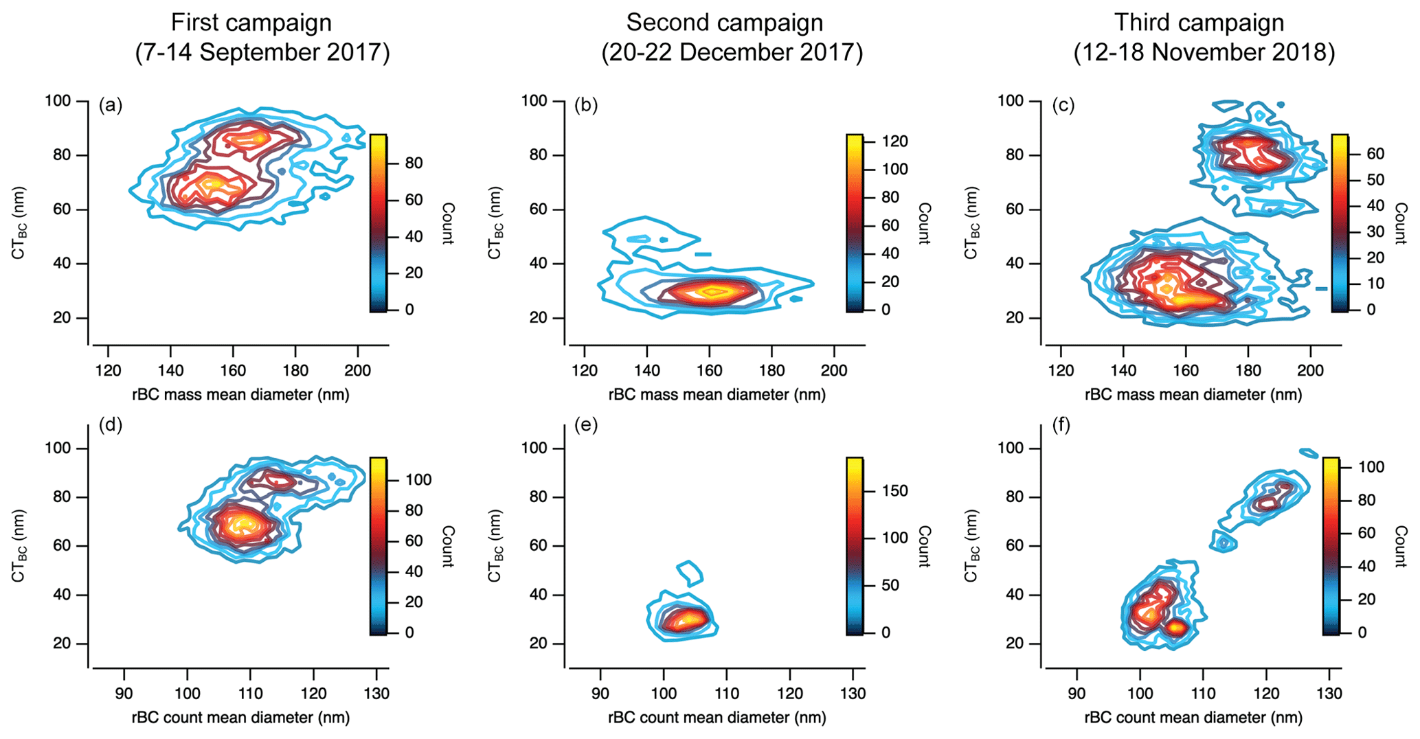
Figure 16Contour plots of count as a function of 1 min mean BC coating thickness (CTBC) and 1 min mean rBC core diameter. This figure can be interpreted as a 2-D joint histogram, converted to a contour plot. Each count represents a single 1 min mean data point. The contours are created based on the 2-D joint histogram that is calculated using a 50×50 grid within the range of all 1 min mean data. Panels (a–c) show the mass mean diameter on the horizontal axes, and panels (d–f) show the count mean diameter.
Within the context of the identifiable sources discussed in previous sections (Sects. 3.1 and S2), it is evident that these distinct clusters in Fig. 16 are strongly influenced by the emissions source type. A BCbb cluster is present in the third campaign (November 2018) when impacts from long-range-transported biomass burning emissions were identified but not in the second campaign (December 2018). Furthermore, a BCff cluster is present in both the second (December 2017) and third campaigns but not in the first campaign (September 2017). This shows that fresh (age < 1 d) fossil fuel emissions from the LA Basin and the surrounding southern California region are characterized by thin coatings and smaller core size, confirming what has also been observed in other past field studies (Laborde et al., 2012; Liu et al., 2014; Krasowsky et al., 2018; Subramanian et al., 2010).
The BCaged,bg cluster (Fig. 16a, d) exhibits two distinct modes within the same cluster. One mode is characterized by a peak CTBC (CMD) that is ∼20 nm (∼10 nm) larger than the other mode. Within the context of BCaged,bg, this mode is referred to as the larger mode, whereas the other mode with smaller CTBC and CMD is referred to as the smaller mode. Based on past reported measurements of the rBC core size and mixing state, we deduce that the larger and smaller modes are representative of biomass burning BC and fossil fuel BC, respectively (McMeeking et al., 2011a; Laborde et al., 2013; Liu et al., 2014; Sahu et al., 2012; Schwarz et al., 2008a; Krasowsky et al., 2018; Corbin et al., 2018). This suggests that BCaged,bg advecting over the Pacific Ocean during typical meteorological conditions contain rBC from both biomass burning and fossil fuel emissions sources. Aged background air masses are likely to contain aerosol from a mix of sources.
In addition to the emissions source type, atmospheric aging also appears to have an observable effect on the mixing state. Table 2 lists the range of estimated “source-to-receptor” timescales for rBC-containing particles measured during LEO time periods L1 to L10. In short, the first campaign (September 2017) is broadly characterized by source-to-receptor timescales on the order of days to a week; the second campaign (December 2017) is characterized by timescales of less than 1 d; and the third campaign (November 2018) is characterized by timescales of less than 1 d for the first 4 d of the campaign and timescales of approximately days to a week for the last 2 d of the campaign.
With regards to aging, we first observe that BCff particles do not develop thick coatings within the timescales observed in this study. This suggests that a timescale of less than 1 d is not sufficient to thickly coat rBC-containing particles from fossil fuel combustion in the lower boundary layer, in the southern California region. Although a modestly higher CTBC is observed during urban-dominated time periods, relative to CTBC∼0 nm observed by Krasowsky et al. (2018) inside the LA Basin, this is likely due to the effects of local biomass burning emissions mixing into the broader urban plume in both December 2017 and November 2018, as discussed above (also see Sect. S2). While we observed mostly thinly coated BC from time periods dominated by fossil fuel emissions, we acknowledge that the timescale required to acquire coatings on BC will likely differ by location because of variations in meteorology, pollution concentrations, and emission source profiles.
On the other hand, BCbb was generally more thickly coated, although the time evolution of the mixing state could not be quantified directly in this study. Fresh BCbb had slightly lower CTBC compared with that of aged BCbb (e.g., L3 versus L9) but higher CTBC compared with that of fresh BCff (e.g., L3 versus L4). The overall higher CTBC for aged BCbb relative to fresh BCbb indicates that significant coating formation can occur within timescales of ∼1 d to ∼1 week for BCbb, even after rapid coating formation that occurs soon after emission. An important caveat is that CTBC of BCbb may not be monotonically increasing over time. Past studies have observed rapid coating of BCbb within 1 d to more than 100 nm (Perring et al., 2017; Morgan et al., 2020), but we observed a median CTBC of 47.7 nm for L3, which suggests that CTBC for BCbb might decrease during atmospheric transport under certain conditions and could again increase later at longer timescales (e.g., median CTBC of 54.0 nm for L9), although we would need simultaneous measurements near the point of biomass burning emissions in order to confirm this for a specific plume. Further research is necessary to confirm this process in more field measurements as well as to determine the various mechanisms that may be driving the potential loss of rBC coating in biomass burning plumes. We make no definitive claims about the rate of change of CTBC for BCbb throughout atmospheric transport because we measured CTBC at one location. Nonetheless, our measurements suggest that CTBC for fresh southern Californian BCbb was generally lower than CTBC for aged northern Californian BCbb.
The contour plots for the first campaign (September 2017), shown in Fig. 16a and d, offer additional perspective on how aging can affect the rBC mixing state within well-aged background air masses over longer aging timescales (∼ days to a week). The first notable feature of the BCaged,bg cluster is that the smaller mode is significantly more coated than the BCff clusters found in Fig. 16 for the second (December 2017) and third (November 2018) campaigns. The peak of the smaller mode of the BCaged,bg cluster is at least ∼35 nm higher than the peak of the respective BCff clusters in Fig. 16b, c, e, and f. Assuming that this smaller mode represents fossil-fuel-influenced BC (e.g., urban, ship, and aviation emissions), this confirms that while BCff may not become thickly coated within 1 d, it seems to acquire coatings over longer timescales.
The evolution of the rBC mixing state and rBC size distribution has important implications for accurately assessing the regional climate benefits of black carbon reductions, particularly in California, and also for reducing uncertainty in global radiative forcing of BC. Understanding the impact of varying emissions source types and atmospheric aging in different regional contexts is crucial for accurately quantifying the enhancement of BC light absorption and also for determining the BC lifetime in the atmosphere because hygroscopic coating material can enhance the particle's susceptibility to wet deposition (Zhang et al., 2015). The rBC mixing state results from this study add to a growing body of evidence that suggests that biomass burning emissions and longer aging timescales generally lead to more thickly coated rBC particles. These results also emphasize the need for more field measurements of the rBC mixing state in various regions around the world to further understand how different emissions source profiles and atmospheric aging ultimately effect rBC physical properties in various, real-world atmospheric contexts.
3.8 Comparison to past studies quantifying CTBC using the SP2
Overall, the range of CTBC calculated in this study is in agreement with reported values from past studies. Table 3 presents a comprehensive list of CTBC values from various studies, categorized by the dominant emissions source type and sorted alphabetically by first author name.
Table 3Summary table of rBC coating thickness values reported in previous studies using the SP2.

a The range of values shown represent the approximate range of the mean CTBC. b The absolute coating thickness was calculated from the ratio of rBC core diameter to particle mobility diameter as presented in the study. Note: a dash (“–”) indicates that the value was not reported or that it could not be identified.
For BCbb, the mean CTBC ranged between ∼40 and 70 nm in this study. This range overlaps with the range of values reported by Morgan et al. (2020), Pan et al. (2017), Sahu et al. (2012), Schwarz et al. (2008a), and Sedlacek et al. (2012). For BCff, the mean CTBC ranged between ∼5 and 15 nm in this study. This range overlaps with the range of values reported by Krasowsky et al. (2018), Laborde et al. (2012), Liu et al. (2014), Sahu et al. (2012), McMeeking et al. (2011a), Corbin et al. (2018), and Schwarz et al. (2008a). For BCaged,bg, the mean CTBC was ∼60 nm in this study. This value falls within the range of values reported by Laborde et al. (2013), Schwarz et al. (2008a), and Shiraiwa et al. (2008).
An important caveat to note when making inter-study comparisons is that the studies that reported higher CTBC ranges (relative to this study) tended to have a lower value for the lower rBC core diameter threshold. For example, Gong et al. (2016) reports a CTBC range of 110–300 nm for biomass burning emissions using an rBC core diameter range of 80–180 nm. The scattering detection limit is accurate down to ∼170 nm for the SP2, which implies that the inclusion of particles with rBC core sizes smaller than 170 nm will bias the average CTBC values higher because smaller rBC particles with optical diameters below the scattering detection will not be included in the LEO analysis. Dahlkötter et al. (2014), Gong et al. (2016), Perring et al. (2017), Taylor et al. (2014), Cheng et al. (2018), Metcalf et al. (2012), Raatikainen et al. (2015), and Sharma et al. (2017) all reported CTBC for rBC-containing particles in a size range that includes rBC cores smaller than 170 nm. There is value in reporting CTBC for rBC particles with core sizes smaller than 170 nm because it will show the relative abundance of coated rBC-containing particles exceeding the lower scattering detection limit, but care must be taken when comparing CTBC values calculated with varying rBC core size restrictions.
For future studies using the SP2, we suggest that, at a minimum, the rBC core size range be explicitly stated if CTBC is being quantified and reported. Furthermore, it would be useful to establish some standardized guidelines for reporting CTBC so that future inter-study comparisons can serve as reliable benchmarks. As shown in Fig. S22 and discussed earlier, the range of rBC core diameters used for the calculation of CTBC has a significant effect on the CTBC statistics. These ranges must be considered in order to accurately represent the physical parameterization of BC mixing state and size distributions in models.
This study investigates the concentration, size distribution, and mixing state of rBC on Catalina Island (∼70 km southwest of Los Angeles) using a single-particle soot photometer (SP2). Measurements were taken during three separate campaigns with varying meteorological conditions and emission sources, in September 2017, December 2017, and November 2018. During the first campaign (7 to 14 September 2017), westerly winds dominated; thus, the sampling location was upwind of the dominant regional sources of BC (i.e., urban emissions from the Los Angeles Basin). The measurements from the first campaign were largely characteristic of well-aged background levels of rBC over the Pacific Ocean, away from the broader urban Los Angeles plume (BCaged,bg). During the second and third campaigns (20 to 22 December 2017 and 12 to 18 November 2018, respectively), due to atypical Santa Ana wind conditions, we measured biomass burning rBC (BCbb) from large wildfires in California and fossil fuel rBC (BCff) from the Los Angeles Basin. Furthermore, during the third campaign, rBC from the Camp Fire in northern California was measured, allowing us to compare the mixing state of aged BCbb (from Camp Fire) to fresher rBC (from southern California fires and urban Los Angeles emissions). The measurements from these three campaigns showed that rBC physical properties (the rBC core size and mixing state) were influenced by (i) the emissions source type and (ii) atmospheric aging.
BCbb generally had larger core diameters than BCff. The MMD (CMD) of BCbb was observed to be ∼180 nm (120 nm), whereas the MMD (CMD) of BCff was observed to be ∼160 nm (100 nm). BCaged,bg showed a bimodal rBC core size distribution, with MMD (CMD) peaks at ∼170 nm (115 nm) for the larger mode and at ∼153 nm (109 nm) for the smaller mode. The bimodal rBC core size distribution from the aged background during the first campaign (September 2017) showed that background rBC above the Pacific Ocean during typical meteorological conditions was likely from a mix of both fossil fuel and biomass burning emissions.
We found that the emissions source type also strongly affected the rBC mixing state. On average, BCff was either uncoated or very thinly coated, with a mean coating thickness (CTBC) ranging from ∼5 to 15 nm and a mean fraction of thickly coated particles (fBC) of less than 0.15. In contrast, BCbb was more thickly coated, with a mean CTBC ranging from ∼40 to 70 nm and fBC ranging from ∼0.23 to 0.47. BCaged,bg was characterized by a mean CTBC of ∼60 nm and fBC of ∼0.27, further confirming that both biomass burning and urban emission sources were likely mixed in these aged background air masses.
We also assessed the effect of aging on both BCbb and BCff. For BCff, we observed that timescales of less than 1 d were not sufficient for fossil fuel rBC particles to become thickly coated. This is in direct contrast to BCbb, which has been shown in previous studies to acquire thick coatings within hours or even minutes, near the source of emissions. For BCbb, we observed higher values of fBC and CTBC during periods that included contributions from the Camp Fire in northern California, compared with periods of fresh biomass burning impacts from local southern California fires (e.g., L3). The average CTBC during the period impacted by the Camp Fire was ∼18 nm higher than the average CTBC during L3, when we identified southern California fires as the main emission source. Likewise, we also observed an increased CTBC with aging for BCff, by comparing the aged BCff mode of the BCaged,bg distribution to fresh BCff during periods when emissions from the LA Basin dominated. We found that coatings on BCff within BCaged,bg were ∼35 nm thicker than BCff from fresh LA Basin emissions. Overall, our measurements suggest that aging increases the coating thickness on both BCff and BCbb, which is consistent with previous research. We did not quantify the rate of change of coating thickness because we were unable to track the evolution of the mixing state during source-to-receptor transport.
The measurements reported in this study agree with past research that investigated the impacts of source type and aging on rBC physical properties. This study further highlights the complexity of the rBC mixing state and demonstrates how meteorology, the emission source type, and atmospheric aging can affect the size distribution and mixing state of BC, even within the same region. Further measurements of rBC physical properties, along with pollutant measurements that allow for robust source apportionment, would improve our understanding of BC mixing state in various regions with different atmospheric contexts. Given that we identified less than 20 studies that quantify CTBC using the LEO method, this study confirms that further measurements are necessary to narrow the quantitative bounds of rBC mixing state in our climate system, which has important implications for the BC absorption enhancement and atmospheric lifetime. We also suggest that future studies further examine the BC mixing state as a function of altitude as well as the role of combustion conditions on mixing state (e.g., flaming versus smoldering), especially in real-world field measurements.
Processed data are available at the following Harvard Dataverse repository: https://dataverse.harvard.edu/dataverse/catalina_rbc_2017_2018 (last access: November 2020) (Harvard Dataverse, 2020).
The DOI citations for individual datasets are as follows:
-
Ko (2019a), https://doi.org/10.7910/DVN/UJAGHY;
-
Ko (2019b), https://doi.org/10.7910/DVN/AAYMHH;
-
Ko (2019c), https://doi.org/10.7910/DVN/CIMVS4.
Due to the extremely large file sizes for the raw SP2 data, they are not publicly available, but they may be made available upon request to the corresponding author.
CAMS model output showing the Camp Fire and southern California plumes during the November 2017 campaign are available at https://doi.org/10.5446/42893 (Ko, 2019d). NASA MODIS images showing the Camp Fire plume during the November 2017 campaign are available at https://doi.org/10.5446/42892 (Ko, 2019e). CAMS model output showing the Camp Fire plume reaching southern California during the December 2018 campaign are available at https://doi.org/10.5446/42943 (Ko, 2019f). Large-scale circulation of aerosols off the California coast during the December 2018 Campaign are available at https://doi.org/10.5446/42942 (Ko, 2019g).
The supplement related to this article is available online at: https://doi.org/10.5194/acp-20-15635-2020-supplement.
Authors JK, TK, and GBW designed the study. JK and TK performed the field measurements. JK and GBW carried out the data analysis. JK and GBW wrote and edited the paper. TK provided technical guidance on field measurements and data analysis.
The authors declare that they have no conflict of interest.
This research was supported by the National Science Foundation (under CAREER grant no. CBET-1752522). This research was also funded in part by the Indo-US Science and Technology Forum.
We acknowledge the use of data from the European Centre for Medium-Range Weather Forecasts (ECMWF). Neither the European Commission nor ECMWF is responsible for any use that may be made of the information it contains.
We acknowledge the NOAA Air Resources Laboratory (ARL) for the provision of the HYSPLIT transport and dispersion model and/or READY website (http://www.ready.noaa.gov, last access: 30 April 2020) used in this publication.
We acknowledge the use of imagery from the NASA Worldview application (https://worldview.earthdata.nasa.gov/, last access: 26 August 2019), part of the NASA Earth Observing System Data and Information System (EOSDIS).
This research has been supported by the National Science Foundation (grant no. CBET-1752522) and the Indo-US Science and Technology Forum (IUSSTF/WAQM-Air Quality Project-IISc Bangalore/2017).
This paper was edited by Philip Stier and reviewed by two anonymous referees.
Adachi, K., Chung, S. H., and Buseck, P. R.: Shapes of soot aerosol particles and implications for their effects on climate, J. Geophys. Res.-Atmos., 115, 1–9, https://doi.org/10.1029/2009JD012868, 2010.
Adachi, K., Moteki, N., Kondo, Y., and Igarashi, Y.: Mixing states of light-absorbing particles measured using a transmission electron microscope and a single-particle soot photometer in Tokyo, Japan, J. Geophys. Res., 121, 9153–9164, https://doi.org/10.1002/2016JD025153, 2016.
Akagi, S. K., Craven, J. S., Taylor, J. W., McMeeking, G. R., Yokelson, R. J., Burling, I. R., Urbanski, S. P., Wold, C. E., Seinfeld, J. H., Coe, H., Alvarado, M. J., and Weise, D. R.: Evolution of trace gases and particles emitted by a chaparral fire in California, Atmos. Chem. Phys., 12, 1397–1421, https://doi.org/10.5194/acp-12-1397-2012, 2012.
Baumgardner, D., Kok, G. L., and Raga, G. B.: On the diurnal variability of particle properties related to light absorbing carbon in Mexico City, Atmos. Chem. Phys., 7, 2517–2526, https://doi.org/10.5194/acp-7-2517-2007, 2007.
Beccario, C.: Earth: a visualization of global weather conditions, available at: https://earth.nullschool.net/, last access: 26 August 2019.
Bond, T. C. and Bergstrom, R. W.: Light absorption by carbonaceous particles: An investigative review, Aerosol Sci. Tech., 40, 27–67, https://doi.org/10.1080/02786820500421521, 2006.
Bond, T. C., Doherty, S. J., Fahey, D. W., Forster, P. M., Berntsen, T., Deangelo, B. J., Flanner, M. G., Ghan, S., Kärcher, B., Koch, D., Kinne, S., Kondo, Y., Quinn, P. K., Sarofim, M. C., Schultz, M. G., Schulz, M., Venkataraman, C., Zhang, H., Zhang, S., Bellouin, N., Guttikunda, S. K., Hopke, P. K., Jacobson, M. Z., Kaiser, J. W., Klimont, Z., Lohmann, U., Schwarz, J. P., Shindell, D., Storelvmo, T., Warren, S. G., and Zender, C. S.: Bounding the role of black carbon in the climate system: A scientific assessment, J. Geophys. Res.-Atmos., 118, 5380–5552, https://doi.org/10.1002/jgrd.50171, 2013.
Cappa, C. D., Onasch, T. B., Massoli, P., Worsnop, D. R., Bates, T. S., Cross, E. S., Davidovits, P., Hakala, J., Hayden, K. L., Jobson, B. T., Kolesar, K. R., Lack, D. A., Lerner, B. M., Li, S. M., Mellon, D., Nuaaman, I., Olfert, J. S., Petäjä, T., Quinn, P. K., Song, C., Subramanian, R., Williams, E. J., and Zaveri, R. A.: Radiative absorption enhancements due to the mixing state of atmospheric black carbon, Science, 337, 1078–1081, https://doi.org/10.1126/science.1223447, 2012.
CBS Los Angeles: Danielle Gersh's Weather Forecast (Dec. 20), available at: https://youtu.be/p8dEJ-qoPwA (last access: 26 August 2019), 2017a.
CBS Los Angeles: Evelyn Taft's Weather Forecast (Dec. 20), available at: https://youtu.be/gDH73gLbGDk (last access: 26 August 2019), 2017b.
CBS Los Angeles: Danielle Gersh's Weather Forecast (Dec. 21), available at: https://youtu.be/j_0P09YZuKc (last access: 26 August 2019), 2017c.
CBS Los Angeles: Garth Kemp's Weather Forecast (Dec. 21), available at: https://youtu.be/vpv65O1MP0A (last access: 26 August 2019), 2017d.
CBS Los Angeles: Evelyn Taft's Weather Forecast (Dec. 22), available at: https://youtu.be/I7KkZiduQq4 (last access: 26 August 2019), 2017e.
CBS Los Angeles: Markina Brown's Weather Forecast (Dec. 22), available at: https://youtu.be/N7htXoFLVcw (last access: 26 August 2019), 2017f.
Cheng, Y., Li, S. M., Gordon, M., and Liu, P.: Size distribution and coating thickness of black carbon from the Canadian oil sands operations, Atmos. Chem. Phys., 18, 2653–2667, https://doi.org/10.5194/acp-18-2653-2018, 2018.
Corbin, J. C., Pieber, S. M., Czech, H., Zanatta, M., Jakobi, G., Massabò, D., Orasche, J., El Haddad, I., Mensah, A. A., Stengel, B., Drinovec, L., Mocnik, G., Zimmermann, R., Prévôt, A. S. H., and Gysel, M.: Brown and Black Carbon Emitted by a Marine Engine Operated on Heavy Fuel Oil and Distillate Fuels: Optical Properties, Size Distributions, and Emission Factors, J. Geophys. Res.-Atmos., 123, 6175–6195, https://doi.org/10.1029/2017JD027818, 2018.
Dahlkötter, F., Gysel, M., Sauer, D., Minikin, A., Baumann, R., Seifert, P., Ansmann, A., Fromm, M., Voigt, C., and Weinzierl, B.: The Pagami Creek smoke plume after long-range transport to the upper troposphere over Europe – Aerosol properties and black carbon mixing state, Atmos. Chem. Phys., 14, 6111–6137, https://doi.org/10.5194/acp-14-6111-2014, 2014.
Gao, R. S., Schwarz, J. P., Kelly, K. K., Fahey, D. W., Watts, L. A., Thompson, T. L., Spackman, J. R., Slowik, J. G., Cross, E. S., Han, J. H., Davidovits, P., Onasch, T. B., and Worsnop, D. R.: A novel method for estimating light-scattering properties of soot aerosols using a modified single-particle soot photometer, Aerosol Sci. Tech., 41, 125–135, https://doi.org/10.1080/02786820601118398, 2007.
Gong, X., Zhang, C., Chen, H., Nizkorodov, S. A., Chen, J., and Yang, X.: Size distribution and mixing state of black carbon particles during a heavy air pollution episode in Shanghai, Atmos. Chem. Phys., 16, 5399–5411, https://doi.org/10.5194/acp-16-5399-2016, 2016.
Harvard Dataverse: Catalina Island rBC Measurements 2017–2018 (University of Southern California), available at: https://dataverse.harvard.edu/dataverse/catalina_rbc_2017_2018, last access: November 2020.
He, C., Liou, K.-N., Takano, Y., Zhang, R., Levy Zamora, M., Yang, P., Li, Q., and Leung, L. R.: Variation of the radiative properties during black carbon aging: theoretical and experimental intercomparison, Atmos. Chem. Phys., 15, 11967–11980, https://doi.org/10.5194/acp-15-11967-2015, 2015.
Hughes, L. S., Allen, J. O., Bhave, P., Kleeman, M. J., Cass, G. R., Liu, D. Y., Fergenson, D. P., Morrical, B. D., and Prather, K. A.: Evolution of atmospheric particles along trajectories crossing the Los Angeles basin, Environ. Sci. Technol., 34, 3058–3068, https://doi.org/10.1021/es9908671, 2000.
IPCC: Climate Change 2013: The Physical Science Basis, in: Contribution of Working Group I to the Fifth Assessment Report of the Intergovernmental Panel on Climate Change, Cambridge University Press, Cambridge, UK and New York, NY, USA, https://doi.org/10.1017/CBO9781107415324, 2013.
Jaross, G.: OMPS-NPP L2 NM Ozone (O3) Total Column swath orbital V2, Goddard Earth Sciences Data and Information Services Center (GES DISC), Greenbelt, MD, USA, https://doi.org/10.5067/0WF4HAAZ0VHK, 2017.
Johnson, G. R., Ristovski, Z. D., D'Anna, B., and Morawska, L.: Hygroscopic behavior of partially volatilized coastal marine aerosols using the volatilization and humidification tandem differential mobility analyzer technique, J. Geophys. Res.-Atmos., 110, 1–14, https://doi.org/10.1029/2004JD005657, 2005.
Justice, C. O., Giglio, L., Korontzi, S., Owens, J., Morisette, J., Roy, D., Descloitres, J., Alleaume, S., Petitcolin, F., and Kaufman, Y. J.: The MODIS fire products, Remote Sens. Environ., 83, 244–262, https://doi.org/10.1016/S0034-4257(02)00076-7, 2002.
Knox, A., Evans, G. J., Brook, J. R., Yao, X., Jeong, C. H., Godri, K. J., Sabaliauskas, K., and Slowik, J. G.: Mass absorption cross-section of ambient black carbon aerosol in relation to chemical age, Aerosol Sci. Tech., 43, 522–532, https://doi.org/10.1080/02786820902777207, 2009.
Ko, J.: Time Series Data for Catalina Island rBC Measurements 2017–2018, Harvard Dataverse, V1, https://doi.org/10.7910/DVN/UJAGHY, 2019a.
Ko, J.: rBC Coating Thickness from Catalina Island rBC Measurements 2017–2018, Harvard Dataverse, V2, https://doi.org/10.7910/DVN/AAYMHH, 2019b.
Ko, J.: rBC Size Distribution from Catalina Island rBC Measurements 2017–2018, Harvard Dataverse, V1, https://doi.org/10.7910/DVN/CIMVS4, 2019c.
Ko, J.: CAMS model output showing the Camp Fire and Southern California plumes during the November 2017 campaign, Copernicus Atmosphere Monitoring Service (CAMS), Beccario, Cameron (earth.nullschool), https://doi.org/10.5446/42893, 2019d.
Ko, J.: NASA MODIS images showing the Camp Fire plume during the November 2017 campaign, National Aeronautics and Space Administration (NASA), https://doi.org/10.5446/42892, 2019e.
Ko, J.: CAMS model output showing the Camp Fire plume reaching Southern California during the December 2018 campaign, Copernicus Atmosphere Monitoring Service (CAMS), Beccario, Cameron (earth.nullschool), https://doi.org/10.5446/42943, 2019f.
Ko, J.: Large-scale circulation of aerosols off the California coast during the December 2018 Campaign, Copernicus Atmosphere Monitoring Service (CAMS), Beccario, Cameron (earth.nullschool), https://doi.org/10.5446/42942, 2019g.
Kondo, Y., Matsui, H., Moteki, N., Sahu, L., Takegawa, N., Kajino, M., Zhao, Y., Cubison, M. J., Jimenez, J. L., Vay, S., Diskin, G. S., Anderson, B., Wisthaler, A., Mikoviny, T., Fuelberg, H. E., Blake, D. R., Huey, G., Weinheimer, A. J., Knapp, D. J., and Brune, W. H.: Emissions of black carbon, organic, and inorganic aerosols from biomass burning in North America and Asia in 2008, J. Geophys. Res.-Atmos., 116, 1–25, https://doi.org/10.1029/2010JD015152, 2011.
Krasowsky, T. S., McMeeking, G. R., Wang, D., Sioutas, C., and Ban-Weiss, G. A.: Measurements of the impact of atmospheric aging on physical and optical properties of ambient black carbon particles in Los Angeles, Atmos. Environ., 142, 496–504, https://doi.org/10.1016/j.atmosenv.2016.08.010, 2016.
Krasowsky, T. S., Mcmeeking, G. R., Sioutas, C., and Ban-Weiss, G.: Characterizing the evolution of physical properties and mixing state of black carbon particles: From near a major highway to the broader urban plume in Los Angeles, Atmos. Chem. Phys., 18, 11991–12010, https://doi.org/10.5194/acp-18-11991-2018, 2018.
Laborde, M., Mertes, P., Zieger, P., Dommen, J., Baltensperger, U., and Gysel, M.: Sensitivity of the Single Particle Soot Photometer to different black carbon types, Atmos. Meas. Tech., 5, 1031–1043, https://doi.org/10.5194/amt-5-1031-2012, 2012.
Laborde, M., Crippa, M., Tritscher, T., Jurányi, Z., Decarlo, P. F., Temime-Roussel, B., Marchand, N., Eckhardt, S., Stohl, A., Baltensperger, U., Prévôt, A. S. H., Weingartner, E., and Gysel, M.: Black carbon physical properties and mixing state in the European megacity Paris, Atmos. Chem. Phys., 13, 5831–5856, https://doi.org/10.5194/acp-13-5831-2013, 2013.
Liu, D., Flynn, M., Gysel, M., Targino, A., Crawford, I., Bower, K., Choularton, T., Jur̈nyi, Z., Steinbacher, M., Ḧglin, C., Curtius, J., Kampus, M., Petzold, A., Weingartner, E., Baltensperger, U., and Coe, H.: Single particle characterization of black carbon aerosols at a tropospheric alpine site in Switzerland, Atmos. Chem. Phys., 10, 7389–7407, https://doi.org/10.5194/acp-10-7389-2010, 2010.
Liu, D., Allan, J. D., Young, D. E., Coe, H., Beddows, D., Fleming, Z. L., Flynn, M. J., Gallagher, M. W., Harrison, R. M., Lee, J., Prevot, A. S. H., Taylor, J. W., Yin, J., Williams, P. I., and Zotter, P.: Size distribution, mixing state and source apportionment of black carbon aerosol in London during winter time, Atmos. Chem. Phys., 14, 10061–10084, https://doi.org/10.5194/acp-14-10061-2014, 2014.
McMeeking, G. R., Hamburger, T., Liu, D., Flynn, M., Morgan, W. T., Northway, M., Highwood, E. J., Krejci, R., Allan, J. D., Minikin, A., and Coe, H.: Black carbon measurements in the boundary layer over western and northern Europe, Atmos. Chem. Phys., 10, 9393–9414, https://doi.org/10.5194/acp-10-9393-2010, 2010.
McMeeking, G. R., Good, N., Petters, M. D., McFiggans, G., and Coe, H.: Influences on the fraction of hydrophobic and hydrophilic black carbon in the atmosphere, Atmos. Chem. Phys., 11, 5099–5112, https://doi.org/10.5194/acp-11-5099-2011, 2011a.
McMeeking, G. R., Morgan, W. T., Flynn, M., Highwood, E. J., Turnbull, K., Haywood, J., and Coe, H.: Black carbon aerosol mixing state, organic aerosols and aerosol optical properties over the United Kingdom, Atmos. Chem. Phys., 11, 9037–9052, https://doi.org/10.5194/acp-11-9037-2011, 2011b.
Metcalf, A. R., Craven, J. S., Ensberg, J. J., Brioude, J., Angevine, W., Sorooshian, A., Duong, H. T., Jonsson, H. H., Flagan, R. C., and Seinfeld, J. H.: Black carbon aerosol over the Los Angeles Basin during CalNex, J. Geophys. Res.-Atmos., 117, 1–24, https://doi.org/10.1029/2011JD017255, 2012.
Morgan, W. T., Allan, J. D., Bauguitte, S., Darbyshire, E., Flynn, M. J., Lee, J., Liu, D., Johnson, B., Haywood, J., Longo, K. M., Artaxo, P. E., and Coe, H.: Transformation and ageing of biomass burning carbonaceous aerosol over tropical South America from aircraft in situ measurements during SAMBBA, Atmos. Chem. Phys., 20, 5309–5326, https://doi.org/10.5194/acp-20-5309-2020, 2020.
Moteki, N. and Kondo, Y.: Effects of mixing state on black carbon measurements by laser-induced incandescence, Aerosol Sci. Tech., 41, 398–417, https://doi.org/10.1080/02786820701199728, 2007.
Moteki, N. and Kondo, Y.: Method to measure time-dependent scattering cross sections of particles evaporating in a laser beam, J. Aerosol Sci., 39, 348–364, https://doi.org/10.1016/j.jaerosci.2007.12.002, 2008.
Moteki, N., Kondo, Y., and Nakamura, S.: Method to measure refractive indices of small nonspherical particles: Application to black carbon particles, J. Aerosol Sci., 41, 513–521, https://doi.org/10.1016/j.jaerosci.2010.02.013, 2010.
Moteki, N., Kondo, Y., Oshima, N., Takegawa, N., Koike, M., Kita, K., Matsui, H., and Kajino, M.: Size dependence of wet removal of black carbon aerosols during transport from the boundary layer to the free troposphere, Geophys. Res. Lett., 39, 2–5, https://doi.org/10.1029/2012GL052034, 2012.
Moteki, N., Kondo, Y., and Adachi, K.: Identification by single-particle soot photometer of black carbon particles attached to other particles: Laboratory experiments and ground observations in Tokyo, Geophys. Res. Lett., 119, 1031–1043, https://doi.org/10.1002/2013JD020655, 2014.
Pan, X., Kanaya, Y., Taketani, F., Miyakawa, T., Inomata, S., Komazaki, Y., Tanimoto, H., Wang, Z., Uno, I., and Wang, Z.: Emission characteristics of refractory black carbon aerosols from fresh biomass burning: A perspective from laboratory experiments, Atmos. Chem. Phys., 17, 13001–13016, https://doi.org/10.5194/acp-17-13001-2017, 2017.
Perring, A. E., Schwarz, J. P., Markovic, M. Z., Fahey, D. W., Jimenez, J. L., Campuzano-Jost, P., Palm, B. D., Wisthaler, A., Mikoviny, T., Diskin, G., Sachse, G., Ziemba, L., Anderson, B., Shingler, T., Crosbie, E., Sorooshian, A., Yokelson, R., and Gao, R. S.: In situ measurements of water uptake by black carbon-containing aerosol in wildfire plumes, J. Geophys. Res., 122, 1086–1097, https://doi.org/10.1002/2016JD025688, 2017.
Raatikainen, T., Brus, D., Hyvärinen, A. P., Svensson, J., Asmi, E., and Lihavainen, H.: Black carbon concentrations and mixing state in the Finnish Arctic, Atmos. Chem. Phys., 15, 10057–10070, https://doi.org/10.5194/acp-15-10057-2015, 2015.
Ramanathan, V. and Carmichael, G.: Global and regional climate changes due to black carbon, Nat. Geosci., 1, 221–227, https://doi.org/10.1038/ngeo156, 2008.
Sahu, L. K., Kondo, Y., Moteki, N., Takegawa, N., Zhao, Y., Cubison, M. J., Jimenez, J. L., Vay, S., Diskin, G. S., Wisthaler, A., Mikoviny, T., Huey, L. G., Weinheimer, A. J., and Knapp, D. J.: Emission characteristics of black carbon in anthropogenic and biomass burning plumes over California during ARCTAS-CARB 2008, J. Geophys. Res.-Atmos., 117, 1–20, https://doi.org/10.1029/2011JD017401, 2012.
Schwarz, J. P., Gao, R. S., Fahey, D. W., Thomson, D. S., Watts, L. A., Wilson, J. C., Reeves, J. M., Darbeheshti, M., Baumgardner, D. G., Kok, G. L., Chung, S. H., Schulz, M., Hendricks, J., Lauer, A., Kärcher, B., Slowik, J. G., Rosenlof, K. H., Thompson, T. L., Langford, A. O., Loewenstein, M., and Aikin, K. C.: Single-particle measurements of midlatitude black carbon and light-scattering aerosols from the boundary layer to the lower stratosphere, J. Geophys. Res.-Atmos., 111, D16207, https://doi.org/10.1029/2006JD007076, 2006.
Schwarz, J. P., Gao, R. S., Spackman, J. R., Watts, L. A., Thomson, D. S., Fahey, D. W., Ryerson, T. B., Peischl, J., Holloway, J. S., Trainer, M., Frost, G. J., Baynard, T., Lack, D. A., de Gouw, J. A., Warneke, C., and Del Negro, L. A.: Measurement of the mixing state, mass, and optical size of individual black carbon particles in urban and biomass burning emissions, Geophys. Res. Lett., 35, 1–5, https://doi.org/10.1029/2008GL033968, 2008a.
Schwarz, J. P., Spackman, J. R., Fahey, D. W., Gao, R. S., Lohmann, U., Stier, P., Watts, L. A., Thomson, D. S., Lack, D. A., Pfister, L., Mahoney, M. J., Baumgardner, D., Wilson, J. C., and Reeves, J. M.: Coatings and their enhancement of black carbon light absorption in the tropical atmosphere, J. Geophys. Res.-Atmos., 113, 1–10, https://doi.org/10.1029/2007JD009042, 2008b.
Schwarz, J. P., Spackman, J. R., Gao, R. S., Perring, A. E., Cross, E., Onasch, T. B., Ahern, A., Wrobel, W., Davidovits, P., Olfert, J., Dubey, M. K., Mazzoleni, C., and Fahey, D. W.: The detection efficiency of the single particle soot photometer, Aerosol Sci. Tech., 44, 612–628, https://doi.org/10.1080/02786826.2010.481298, 2010.
Schroeder, W., Oliva, P., Giglio, L., and Csiszar, I. A.: The New VIIRS 375 m active fire detection data product: algorithm description and initial assessment, Remote Sens. Environ., 143, 85–96, https://doi.org/10.1016/j.rse.2013.12.008, 2014.
Sedlacek, A. J., Lewis, E. R., Kleinman, L., Xu, J., and Zhang, Q.: Determination of and evidence for non-core-shell structure of particles containing black carbon using the Single-Particle Soot Photometer (SP2), Geophys. Res. Lett., 39, 2–7, https://doi.org/10.1029/2012GL050905, 2012.
Sedlacek, A. J., Lewis, E. R., Onasch, T. B., Lambe, A. T., and Davidovits, P.: Investigation of Refractory Black Carbon-Containing Particle Morphologies Using the Single-Particle Soot Photometer (SP2), Aerosol Sci. Tech., 49, 872–885, https://doi.org/10.1080/02786826.2015.1074978, 2015.
Sharma, S., Leaitch, W. R., Huang, L., Veber, D., Kolonjari, F., Zhang, W., Hanna, S. J., Bertram, A. K., and Ogren, J. A.: An evaluation of three methods for measuring black carbon in Alert, Canada, Atmos. Chem. Phys., 17, 15225–15243, https://doi.org/10.5194/acp-17-15225-2017, 2017.
Shiraiwa, M., Kondo, Y., Moteki, N., Takegawa, N., Miyazaki, Y., and Blake, D. R.: Evolution of mixing state of black carbon in polluted air from Tokyo, Geophys. Res. Lett., 34, 2–6, https://doi.org/10.1029/2007GL029819, 2007.
Shiraiwa, M., Kondo, Y., Moteki, N., Takegawa, N., Sahu, L. K., Takami, A., Hatakeyama, S., Yonemura, S., and Blake, D. R.: Radiative impact of mixing state of black carbon aerosol in Asian outflow, J. Geophys. Res.-Atmos., 113, 1–13, https://doi.org/10.1029/2008JD010546, 2008.
Slowik, J. G., Cross, E. S., Han, J. H., Davidovits, P., Onasch, T. B., Jayne, J. T., Williams, L. R., Canagaratna, M. R., Worsnop, D. R., Chakrabarty, R. K., Moosmüller, H., Arnott, W. P., Schwarz, J. P., Gao, R. S., Fahey, D. W., Kok, G. L., and Petzold, A.: An Inter-Comparison of Instruments Measuring Black Carbon Content of Soot Particles, Aerosol Sci. Tech., 41, 295–314, https://doi.org/10.1080/02786820701197078, 2007.
Soleimanian, E., Mousavi, A., Taghvaee, S., Shafer, M. M., and Sioutas, C.: Impact of secondary and primary particulate matter (PM) sources on the enhanced light absorption by brown carbon (BrC) particles in central Los Angeles, Sci. Total Environ., 705, 135902, https://doi.org/10.1016/j.scitotenv.2019.135902, 2020.
Stein, A. F., Draxler, R. R., Rolph, G. D., Stunder, B. J. B., Cohen, M. D., and Ngan, F.: Noaa's hysplit atmospheric transport and dispersion modeling system, B. Am. Meteorol. Soc., 96, 2059–2077, https://doi.org/10.1175/BAMS-D-14-00110.1, 2015.
Stephens, M., Turner, N., and Sandberg, J.: Particle identification by laser-induced incandescence in a solid-state laser cavity, Appl. Optics, 42, 3726, https://doi.org/10.1364/ao.42.003726, 2003.
Subramanian, R., Kok, G. L., Baumgardner, D., Clarke, A., Shinozuka, Y., Campos, T. L., Heizer, C. G., Stephens, B. B., De Foy, B., Voss, P. B., and Zaveri, R. A.: Black carbon over Mexico: The effect of atmospheric transport on mixing state, mass absorption cross-section, and BC ∕ CO ratios, Atmos. Chem. Phys., 10, 219–237, https://doi.org/10.5194/acp-10-219-2010, 2010.
Taylor, J. W., Allan, J. D., Allen, G., Coe, H., Williams, P. I., Flynn, M. J., Le Breton, M., Muller, J. B. A., Percival, C. J., Oram, D., Forster, G., Lee, J. D., Rickard, A. R., Parrington, M., and Palmer, P. I.: Size-dependent wet removal of black carbon in Canadian biomass burning plumes, Atmos. Chem. Phys., 14, 13755–13771, https://doi.org/10.5194/acp-14-13755-2014, 2014.
Taylor, J. W., Allan, J. D., Liu, D., Flynn, M., Weber, R., Zhang, X., Lefer, B. L., Grossberg, N., Flynn, J., and Coe, H.: Assessment of the sensitivity of core/shell parameters derived using the single-particle soot photometer to density and refractive index, Atmos. Meas. Tech., 8, 1701–1718, https://doi.org/10.5194/amt-8-1701-2015, 2015.
Todey, D. P., Herzmann, D. E., and Takle, G. S.: The Iowa Environmental Mesonet – combining networks into a single network, in: Preprints 6th Symposium on Integrated Observing Systems, Annual Meeting of the American Meteorological Society, 14–17 January 2002, Orlando, FL, USA, 2002.
Torres, O.: OMI/Aura Near UV Aerosol Optical Depth and Single Scattering Albedo 1-orbit L2 Swath 13×24 km V003, Greenbelt, MD, USA, Goddard Earth Sciences Data and Information Services Center (GES DISC), https://doi.org/10.5067/Aura/OMI/DATA2004, 2006.
Wang, Q., Huang, R. J., Cao, J., Han, Y., Wang, G., Li, G., Wang, Y., Dai, W., Zhang, R., and Zhou, Y.: Mixing state of black carbon aerosol in a heavily polluted urban area of China: Implications for light absorption enhancement, Aerosol Sci. Tech., 48, 689–697, https://doi.org/10.1080/02786826.2014.917758, 2014.
Wang, Q., Cao, J., Han, Y., Tian, J., Zhang, Y., Pongpiachan, S., Zhang, Y., Li, L., Niu, X., Shen, Z., Zhao, Z., Tipmanee, D., Bunsomboonsakul, S., Chen, Y., and Sun, J.: Enhanced light absorption due to the mixing state of black carbon in fresh biomass burning emissions, Atmos. Environ., 180, 184–191, https://doi.org/10.1016/j.atmosenv.2018.02.049, 2018.
WHO – World Health Organization: Health effects of black carbon, ISBN 9789289002653, available at: http://www.euro.who.int/__data/assets/pdf_file/0004/162535/e96541.pdf (last access: 26 August 2019), 2012.
Zhang, J., Liu, J., Tao, S., and Ban-Weiss, G. A.: Long-range transport of black carbon to the Pacific Ocean and its dependence on aging timescale, Atmos. Chem. Phys., 15, 11521–11535, https://doi.org/10.5194/acp-15-11521-2015, 2015.