the Creative Commons Attribution 4.0 License.
the Creative Commons Attribution 4.0 License.
 | 25 Nov 2020
Quantifying the emission changes and associated air quality impacts during the COVID-19 pandemic on the North China Plain: a response modeling study
Jia Xing
Siwei Li
Yueqi Jiang
Dian Ding
Zhaoxin Dong
Yun Zhu
Jiming Hao
Quantification of emission changes is a prerequisite for the assessment of control effectiveness in improving air quality. However, the traditional bottom-up method for characterizing emissions requires detailed investigation of emissions data (e.g., activity and other emission parameters) that usually takes months to perform and limits timely assessments. Here we propose a novel method to address this issue by using a response model that provides real-time estimation of emission changes based on air quality observations in combination with emission-concentration response functions derived from chemical transport modeling. We applied the new method to quantify the emission changes on the North China Plain (NCP) due to the COVID-19 pandemic shutdown, which overlapped the Spring Festival (also known as Chinese New Year) holiday. Results suggest that the anthropogenic emissions of NO2, SO2, volatile organic compound (VOC) and primary PM2.5 on the NCP were reduced by 51 %, 28 %, 67 % and 63 %, respectively, due to the COVID-19 shutdown, indicating longer and stronger shutdown effects in 2020 compared to the previous Spring Festival holiday. The reductions of VOC and primary PM2.5 emissions are generally effective in reducing O3 and PM2.5 concentrations. However, such air quality improvements are largely offset by reductions in NOx emissions. NOx emission reductions lead to increases in O3 and PM2.5 concentrations on the NCP due to the strongly VOC-limited conditions in winter. A strong NH3-rich condition is also suggested from the air quality response to the substantial NOx emission reduction. Well-designed control strategies are recommended based on the air quality response associated with the unexpected emission changes during the COVID-19 period. In addition, our results demonstrate that the new response-based inversion model can well capture emission changes based on variations in ambient concentrations and thereby illustrate the great potential for improving the accuracy and efficiency of bottom-up emission inventory methods.
- Article
(3100 KB) - Full-text XML
-
Supplement
(4087 KB) - BibTeX
- EndNote


Accurate estimation of anthropogenic emissions is crucial for atmospheric modeling studies and provides the basis for developing effective air pollution controls (Wang et al., 2010). A comprehensive emission inventory consists of the emission rates of primary particulate matter components and gaseous pollutants and precursors that are allocated over time and space. These inventories are usually developed using bottom-up methods that gather detailed information about source activity and other emission parameters (Wang et al., 2011a; Xing et al., 2013; Li et al., 2017). The challenge is that such an investigation is costly and time-consuming, and therefore the latest emission inventories usually lag current conditions by a year or more. Many studies also apply a top-down methods to constrain emission estimates using satellite retrievals and modeling methods (Tang et al., 2013, 2019; Lu et al., 2015; Miyazaki et al., 2017; Cao et al., 2018; Zhang et al., 2018). In general, the traditional top-down inversion methods use four-dimensional data assimilation (Mendoza-Dominguez and Russell, 2000) or Kalman filter methods (Hartley and Prinn, 1993) combined with sensitivity analysis of chemical transport modeling, like decoupled direct method in three dimensions (Napelenok et al., 2008) or adjoint method (Cao et al., 2018), to optimize the gap between the simulation and observation through adjusting the emission from an a priori estimate. The top-down inversion method can well reflect the change in emissions in a timely manner and thus efficiently estimate emissions at high spatial and temporal resolution to complement bottom-up inventories. Previous inversion studies have focused on individual pollutants that can be measured directly; however, studies are lacking that use top-down methods to estimate emissions of multiple pollutants, including those that cannot be directly measured, such as primary fine particular matter (p-PM2.5).
The ongoing coronavirus disease 2019 (COVID-19) pandemic has led to 4600 deaths in mainland China (by 24 May 2020, https://news.google.com/covid19/, last access: 24 May 2020) and has resulted in a dramatic curtailment of routine economic and social activities. The shutdown of human activities during the COVID-19 pandemic has led to reduced pollutant emissions and possibly improved air quality (Shi and Brasseur, 2020; Wang et al., 2020). Yet according to ambient concentration measurements, heavy PM2.5 pollution still occurred during the COVID-19 period, and formation of secondary pollutants was actually enhanced in China (Li et al., 2020; Huang et al., 2020). Some studies attributed pollution enhancements to atypical weather conditions that are favorable for air pollution formation (Wang and Su, 2020). Meanwhile, the unexpected reduction of anthropogenic emissions due to the COVID-19 shutdown might vary significantly for different sectors and species. For example, emissions from domestic sources might have increased due to a greater demand for home heating and other essential consumptions during periods with stay-at-home orders in effect. Moreover, the coincidence of the COVID-19 shutdown and the Spring Festival in China resulted in large numbers of people confined to their rural or small-city hometowns, where consumption patterns differ greatly from their primary residence in megacities. Relative to previous years, both emissions and meteorological conditions varied simultaneously during the 2020 COVID-19 shutdown, and an accurate estimation of the changes in anthropogenic emissions accounting for meteorological variations is needed to characterize the impacts of COVID-19 on air quality.
Here we propose a novel inversion technique based on a multi-pollutant nonlinear response model to estimate the emission changes on the North China Plain (NCP) during the COVID-19 shutdown. Emission changes for the COVID-19 period are calculated as the difference between emission estimates for actual conditions and hypothetical conditions assuming the shutdown did not occur. The hypothetical emissions are determined by combining top-down emission estimates from before and after the shutdown with estimates of the temporal variation in emissions from a bottom-up emission inventory. Additionally, we estimate the change in emissions associated with the Spring Festival holiday in 2019 to contrast with results for the combined Spring Festival holiday and COVID-19 shutdown in 2020. Finally, we evaluate the impacts on PM2.5 and O3 concentrations of the combined emission changes and for each emitted species to provide insights for the design of effective control strategies in the future.
2.1 Response model to estimate the actual emissions from observed surface concentrations
The principle of the new response-based inversion model (hereafter “the response model”) is to adjust the assumed prior emissions such that concentration predictions match observations. Different from previous top-down methods that apply sensitivity based optimization, this study adopted emission-concentration response functions which provide real-time estimates of the concentrations under various emission scenarios. Therefore it can make the adjustment of emissions match with the observation more straightforwardly by avoiding the calculation of the sensitivities. Meanwhile, the natural linkage exists in air pollutants like PM2.5 and O3 since both pollutants have contributions from common precursors (NOx and volatile organic compound, VOC), similar atmospheric diffusion–advection transport, and chemical oxidation reactions. The advantage of the new method is its ability to represent the nonlinearity of PM2.5 and O3 response to the change in their precursor emissions. Thus, it can assimilate both pollutants simultaneously by keeping the natural linkage. In addition, to address the “ill-posedness” inversion problem, we took advantage of all available observations for multiple pollutants and constrained the adjustment of emissions at provincial scale rather than at each single grid cell. That means we only change total emissions of each province but keep spatial and temporal variation the same as that in the a priori emissions. Such a design makes the new method have a small sensitivity to the change of observation sites due to the use of prior knowledge of the spatial distribution of emissions, which is particularly useful for certain period when observations are not always available across the whole region. However, the new method has limited ability to assimilate concentrations at the edge of the control region and may suffer uncertainties in the spatial and temporal variations which are unable to be adjusted by this method (Xing et al., 20201). Nevertheless, since the study mainly focuses on the relative change of total emissions over the NCP region due to the COVID-19 rather than improving the baseline emissions, our new method is thus more suitable to address such a specific purpose.
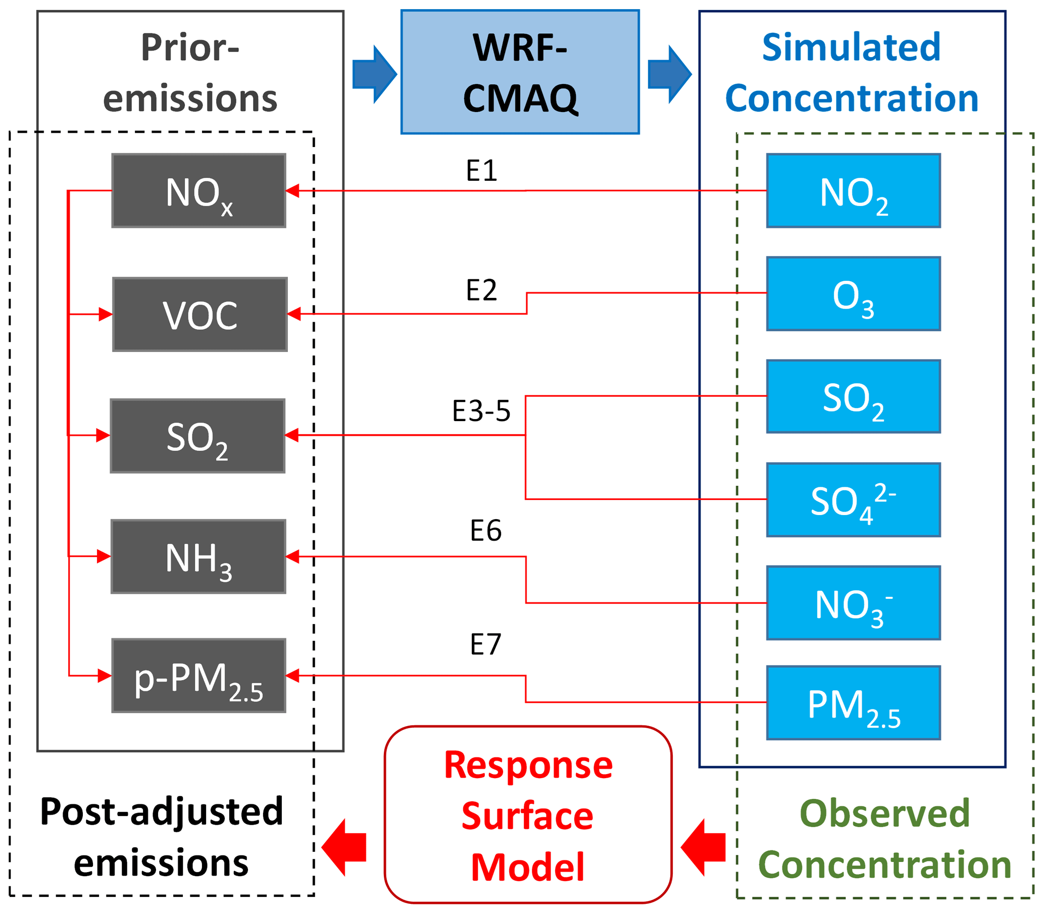
Figure 1The response modeling framework for adjusting the emissions (Eqs. 1–7 are equations used to adjusted emissions, which are detailed in the text).
The core element of the inversion method is a nonlinear response surface model (RSM) that represents the emission-concentration response functions. The framework of the response model is illustrated in Fig. 1. We conduct chemical transport model simulations using prior emissions to get the original simulated concentrations of six pollutants (i.e., NO2; O3; SO2; PM2.5; sulfate, ; and nitrate, ), as well as the response functions derived from the RSM (Xing et al., 2011; Wang et al., 2011b; Xing et al., 2017, 2018). We then adjust the total emission ratio of five pollutants (i.e., NO2, VOC, SO2, NH3 and primary PM2.5) in five provinces of the NCP (i.e., Beijing, Tianjin, Hebei, Shandong and Henan) to estimate the updated simulated concentrations to match with the observations. Since the RSM was originally built based on the 3-D chemical transport model through multiple-emission scenarios by changing total emissions at controlled regions, both local source and non-local transport and transformation have been considered in the assimilation.
Based on our previous knowledge of emission-concentration response relationships, we first adjust NOx emissions such that RSM predictions match NO2 observations (see Eq. 1), since NO2 concentrations have a strong linear relationship with NOx emissions (Xing et al., 2017).
where is the adjusted NOx emissions; is the prior NOx emissions; is the adjustment ratio for NOx emissions; is the observed NO2 concentrations; and is the simulated NO2 concentrations.
Next, we adjust VOC emissions such that RSM predictions match observed O3 concentrations, since O3 concentrations are solely determined by VOC emissions after NOx emissions are determined in the previous step. The adjusted VOC emission ratio (i.e., ) is determined by solving the following equation:
where is the adjusted VOC emissions; is the prior VOC emissions; ΔO3 is the difference between observed O3 concentrations () and simulated O3 concentrations (); and is the response function of O3 concentrations to NOx and VOC emissions.
Although SO2 concentrations are linearly related to SO2 emissions, the chemical transport model overestimates SO2 concentrations and underestimates concentrations due to large uncertainties in simulating the rapid conversion of SO2 to during haze episodes (Zhang et al., 2019). To address this deficiency, we adjusted the SO2 emissions using the observed ratio such that the RSM predictions matched both the observed SO2 and concentrations. Since concentrations are quite linearly related to SO2 emissions when NH3 emissions are at moderate levels (Wang et al., 2011b), we assume that the unaccounted for SO2-to- conversion pathway contributes to differences in the observed and simulated ratios. Under this assumption, simulated SO2 concentrations are overestimated by the same ratio (α) that secondary () concentrations are underestimated (see Eqs. 3 and 4). The primary concentration () was removed from the total concentration in these calculations, because primary is directly emitted and not related to the conversion of SO2 to (see Eq. 4).
The adjusted SO2 emission ratio () is estimated by taking the ratio of observed SO2 () to simulated SO2 () multiplied by α, which accounts for the model deficiency in simulating the rapid conversion of SO2 to . For simplification, here we estimate the α value at a domain and temporal averaged level (i.e., identical across the space and time), though such a ratio might vary with time and space. Also the primary SO4 concentrations were assumed to be correct. The α is smaller than 1 because the observed is usually greater than the simulation. The inclusion of the α may help the response model avoid the underestimation of SO2 emissions.
Using the adjusted NOx, VOC and SO2 emissions from previous steps, we next adjusted NH3 emissions such that RSM predictions of concentrations matched observations:
where , is the adjusted NH3 emissions, and is the prior NH3 emissions.
After updating the emissions of the four gaseous precursors, the secondary portion of PM2.5 was correspondingly determined, including the secondary organic aerosol contributed by the VOC emissions. Finally, the primary PM2.5 emissions were adjusted to provide agreement between simulated and observed total PM2.5 concentrations:
where , is the adjusted primary PM2.5 emissions, and is the prior primary PM2.5 emissions.
The prior emissions used here were based on a bottom-up inventory developed for 2017. Since our study focuses on periods in 2019 and 2020, we first use the response model to adjust the 2017 emission inventory to match the observations during two study periods. The first study period was defined as 1 January–31 March 2019 to capture changes in activity due the Spring Festival. The second study period was defined as the same 3 months in 2020 to capture the COVID-19 shutdown on the NCP, which overlapped the 2020 Spring Festival holiday. We defined three subperiods within the 3 months in each year as pre-shutdown (Period 1), shutdown (Period 2) and post-shutdown (Period 3). The days selected for subperiods differed in 2019 and 2020 due to differences in the dates and lengths of the shutdowns. For 2019, we defined Period 1 as 1–29 January (29 d); Period 2 as 30 January–18 February (20 d), which is a week before and after the 2019 lunar New Year holidays; and Period 3 as 19 February–31 March (41 d). For 2020, we defined Period 1 as 1–22 January (22 d); Period 2 as 23 January–5 March (33 d), which is from the date that Chinese authorities began targeting transportation shutdowns until all human activities began recovering in early March (http://www.gov.cn/index.htm, last access: 24 May 2020); and Period 3 as 6–31 March (26 d). The stage-averaged emissions are corrected by applying a unified change ratio to each pollutant emission at each stage, and the temporal variations such as hourly profiles are kept the same as those in the a priori estimates.
The RSM was developed using ambient concentrations from simulations with the Community Multiscale Air Quality (CMAQ, version 5.2.1) model, which incorporated meteorological fields from the Weather Research and Forecasting (WRF, version 3.8) model. The WRF-CMAQ system was configured as in our previous studies, and model performance for meteorological variables and pollutant concentrations was evaluated (Ding et al., 2019). The RSM was developed following the same design as our previous study (Xing et al., 2018), in which the polynomial response functions for O3, PM2.5 and PM2.5 components were fitted by 40 brute-force CMAQ simulations. Specifically, deep-learning technology was used to fit response surfaces for the 3 months in 2019 and 2020 using CMAQ simulations for baseline and zero-out emissions conditions (see Fig. 2 in Xing et al., 2020b). The response surfaces were developed using year-specific meteorology based on WRF simulations to account for differences in meteorological conditions between 2019 and 2020.
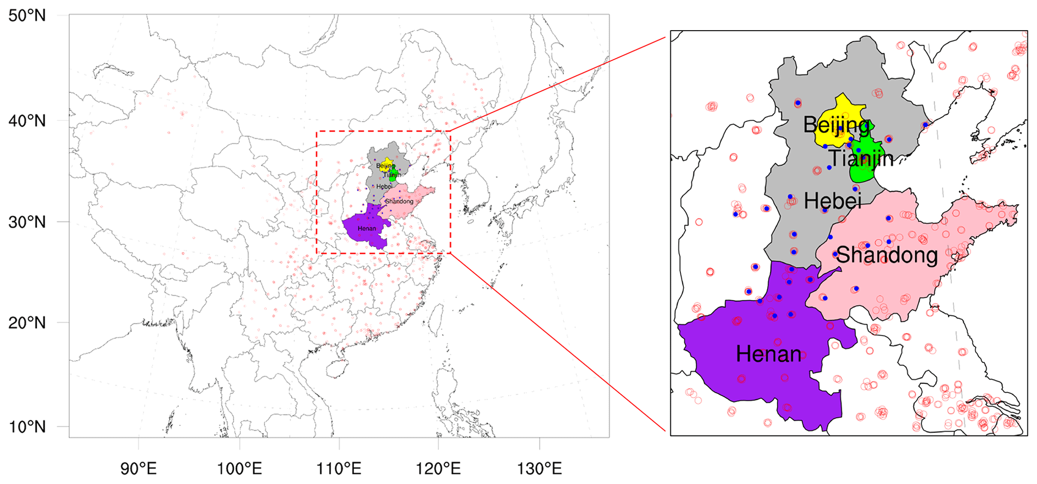
Figure 2Simulation domain and location of observation sites (colored area: five provinces of the North China Plain; red dots: surface monitor sites for NO2, SO2, O3 and PM2.5; blue dots: monitor sites for PM2.5 chemical components).
Measurements of ambient concentrations of NO2, SO2, O3 and PM2.5 were obtained from the China National Environmental Monitoring Centre (http://106.37.208.233:20035/, last access: 24 May 2020). Measurements of PM2.5 chemical components, including and , were provided by the urban PM data analysis platform in the 2+26 cities of Beijing–Tianjin–Hebei and surrounding regions (http://106.37.181.120:9011/bfs, last access: 24 May 2020). All monitoring data were given as hourly averaged concentrations at the monitoring sites shown in Fig. 2. As in our previous RSM studies, daily daytime O3 concentrations were analyzed based on afternoon averages (12:00–18:00 local time), and PM2.5 concentrations were based on daily 24 h averages (Xing et al., 2018). Only data at monitoring sites that covered the 90 % of entire period are considered. Since the monitors sample pollutants at discrete locations and measurements are not available for all days at all sites, provincial average concentrations were used to facilitate adjustments domain-wide for all days in each study period. The provincial average concentrations were calculated using spatially and temporally matched simulated and observed values.
2.2 Hypothetical emissions without shutdown effects
The actual emissions can be derived using observed concentrations and the response model. However, hypothetical emissions under the assumption of no shutdown effects are also needed to estimate the changes in emissions due to the 2019 and 2020 shutdowns. We estimate the hypothetical emissions using the temporal profiles of sectoral emissions from the bottom-up inventory in combination with the derived (actual) emissions for the pre- and post-shutdown periods. We assume that the Spring Festival shutdowns in 2019 have negligible influence on emissions during the periods before and after the shutdown (i.e., Period 1 and Period 3, respectively), while the COVID-19 pandemic in 2020 might have had lag effects after the shutdown due to reduced economic activity or relaxed pollutant controls. However, we concentrate our analysis of COVID-19 impacts on emissions and air quality in the official shutdown period only (Period 2). The hypothetical no-shutdown emissions for Period 2 (noted as Period 2H) are estimated using ratios of emissions for Period 2 and Period 1 and 3 based on the temporal profile (i.e., reflect the monthly variation across a year) of the bottom-up inventory which only reflects the natural evolution of emissions across a year for each sector. It is roughly close to the temporally averaged ratios between Periods 1 and 3, and the exact values depend on the number of days covering in each period. This approach develops hypothetical emissions following the typical variation in emissions without shutdown effects. Note that we use the temporal profile to determine the change in Period 2 emissions relative to Period 1 and 3, and so emissions from both Period 1 and 3 are needed to estimate Period 2H emissions.
The emission changes due to the COVID-19 shutdown can be estimated by taking the difference of emissions in Period 2, derived from the response model, and emissions in Period 2H, estimated from emissions in Period 1 and 3 using the temporal profile of bottom-up sectoral emissions. The impacts of emission changes during the COVID-19 shutdown on PM2.5 and O3 concentrations are then estimated with the RSM. In addition to the combined impacts of emission changes from multiple species, we estimate the impacts of individual pollutant emissions on PM2.5 and O3. Due to the nonlinearity of emission-concentration response functions, the impacts of individual pollutant emissions can vary significantly when other pollutant emissions are changing simultaneously (Xing et al., 2018). To simplify the evaluation, we define an incremental method for analyzing the individual pollutant impacts in this study by adding incremental changes in pollutant emissions to the previous simulation in the following order: NOx, VOC, NH3, SO2 and primary PM2.5, as described in Table 1. The impacts of individual pollutant emissions on O3 and PM2.5 concentrations are then estimated from the difference between the incrementally adjusted simulation and the previous one. Note that this approach is an approximation, and the impacts of individual pollutants could change if a different order is used.
Table 1Sensitivity analysis for quantifying the impacts of individual pollutant emission changes on air quality.
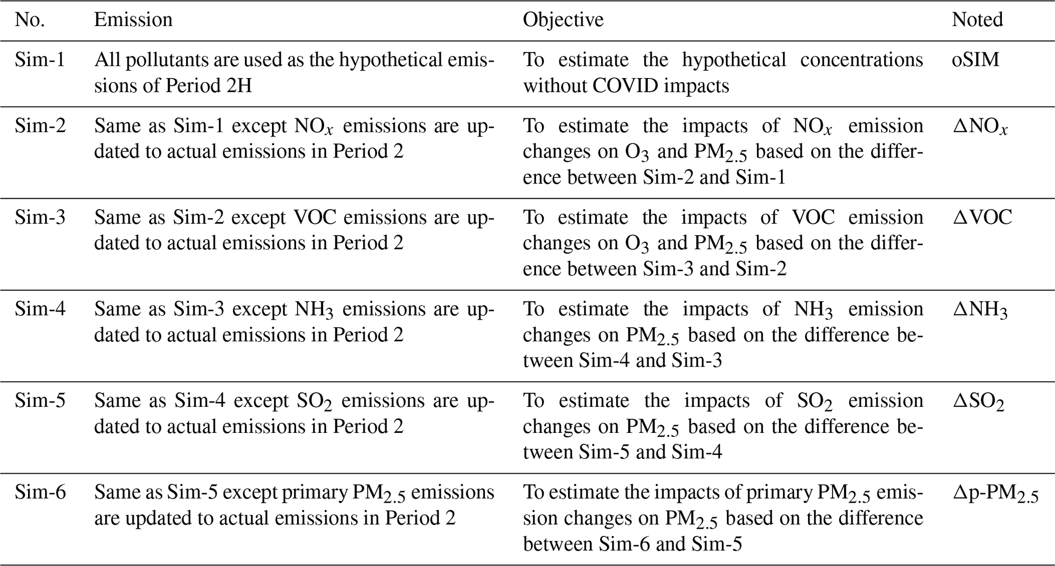
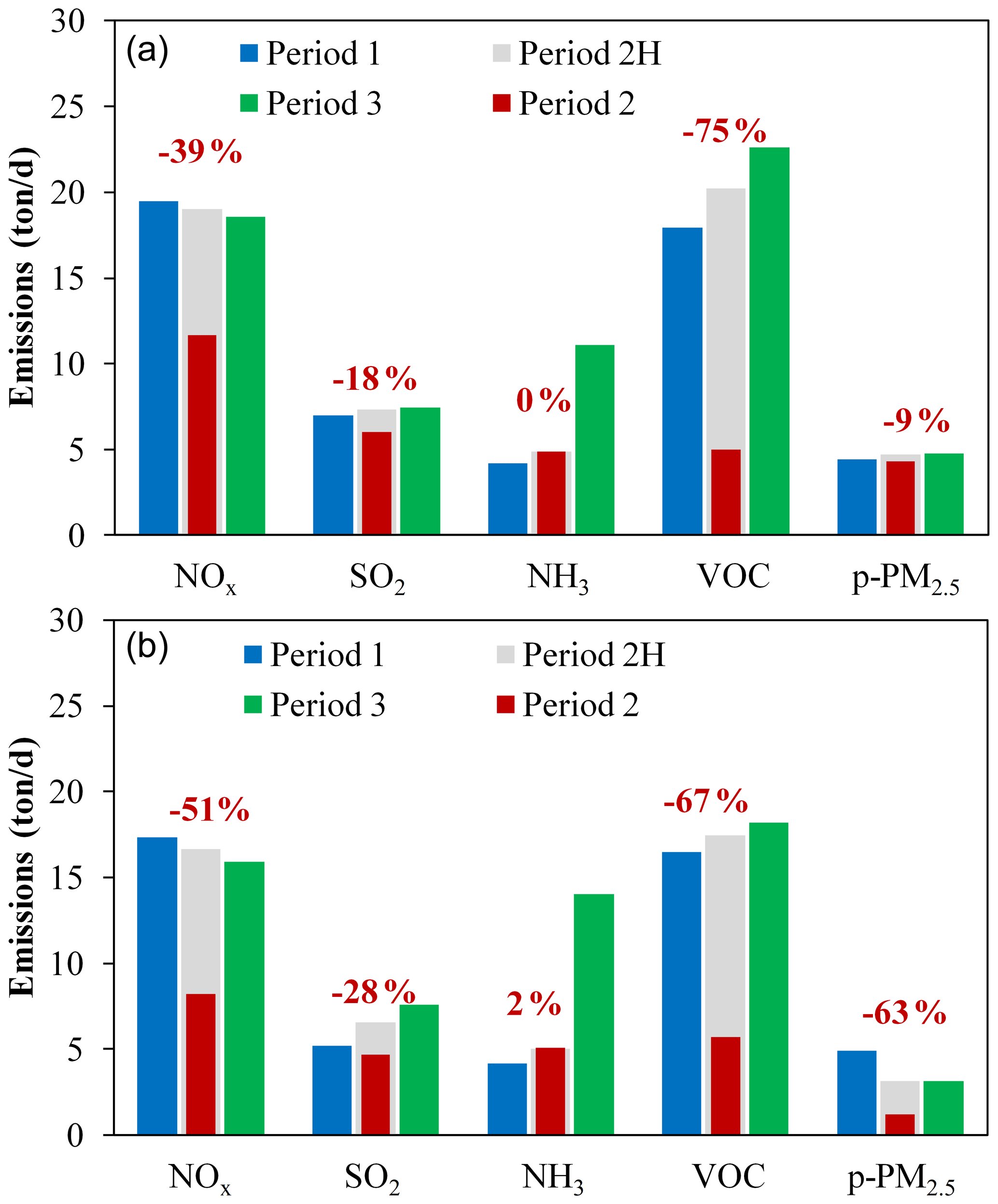
Figure 3Daily emissions during pre-shutdown (Period 1, blue), shutdown (Period 2, red) and post-shutdown (Period 3, green) periods in 2019 and 2020. Period 2H (grey) is the hypothetical emissions without reduced activity during the 2019 holiday or 2020 COVID-19 shutdown; the red number indicates the percent change in emissions due to the shutdown in Period 2.
3.1 Emission changes due to the shutdown
Using the response model, the daily emissions of NOx, VOC, NH3, SO2 and primary PM2.5 on the NCP are estimated for three periods in 2019 and 2020, as summarized in Fig. 3 and detailed in Table 2 by provinces.
For Period 1 before the activity disruptions, the emissions of NOx, SO2 and VOC on the NCP decreased by 11 %, 25 % and 8 % between 2019 and 2020, respectively. These reductions reflect the progress of air pollution controls between 2019 and 2020 and demonstrate the ability of the model to capture emission changes from routine air pollution control actions. The p-PM2.5 emissions also significantly decreased in Beijing–Tianjin–Hebei provinces but increased in Shandong and Henan. The NH3 emissions did not change during this 2-year period, since NH3 is not considered in current policies.
Table 2Daily emissions of five pollutants in NCP provinces based on the response model (unit: kt d−1). p-PM2.5: primary PM2.5.

Activity reductions occurred in Period 2 in both 2019 and 2020, although the shutdown due the Spring Festival in 2019 is much shorter than the COVID-19 shutdown in 2020. The emissions of NOx, SO2 and p-PM2.5 in Period 2 in 2020 are substantially lower than in 2019 (29 %, 22 % and 73 %, respectively). The decreases of NOx and p-PM2.5 for Period 2 between 2019 and 2020 are larger than the decreases for Period 1, which did not experience shutdowns. Such results suggest that the COVID-19 shutdown in 2020 had longer and stronger impacts on emissions than the Spring Festival shutdown in 2019. Interestingly, emissions of NH3 and VOC increased significantly (by 5 % and 14 %) from 2019 to 2020 in Period 2. These changes are likely due to the temporal variations of emissions of both species, which are enhanced in warmer months due to stronger evaporation. Period 2 in 2020 extended farther into the spring (until early March) than Period 2 in 2019 and thus led to increased evaporative emissions of NH3 and VOC. These results also demonstrate the importance of developing emissions with high temporal resolution.
For Period 3 after the shutdown, the decreases of NOx emissions (14 %) are similar to those in Period 1 (11 %), indicating the recovery of the activity. However, the emissions of VOC and p-PM2.5 are much lower in Period 3 in 2020 compared to that in 2019, suggesting lag effects after the COVID-19 shutdown in 2020. In contrast, the small increases of SO2 emissions in 2020 (2 %) might be associated with the extended central heating activity through the end of March in 2020, compared with mid-March in 2019. Higher NH3 emissions in Period 3 in 2020 than 2019 are also due to the larger coverage of warm days in Period 3 of 2020. NH3 emissions show the strongest monthly variations among all pollutants (Fig. 3). Similarly, increases in VOC emissions are also driven by the change of meteorological conditions (i.e., the higher air temperature in March leads to a larger evaporative emissions), though the growth of VOC emissions from Period 1 to Period 3 is reduced by the COVID-19 shutdown in 2020. Such results also demonstrate that the response model can capture the temporal variations of emissions even in cases where emissions are strongly coupled with meteorological conditions.
Table 3The shutdown impacts on the emission of five pollutants in NCP provinces. p-PM2.5: primary PM2.5.
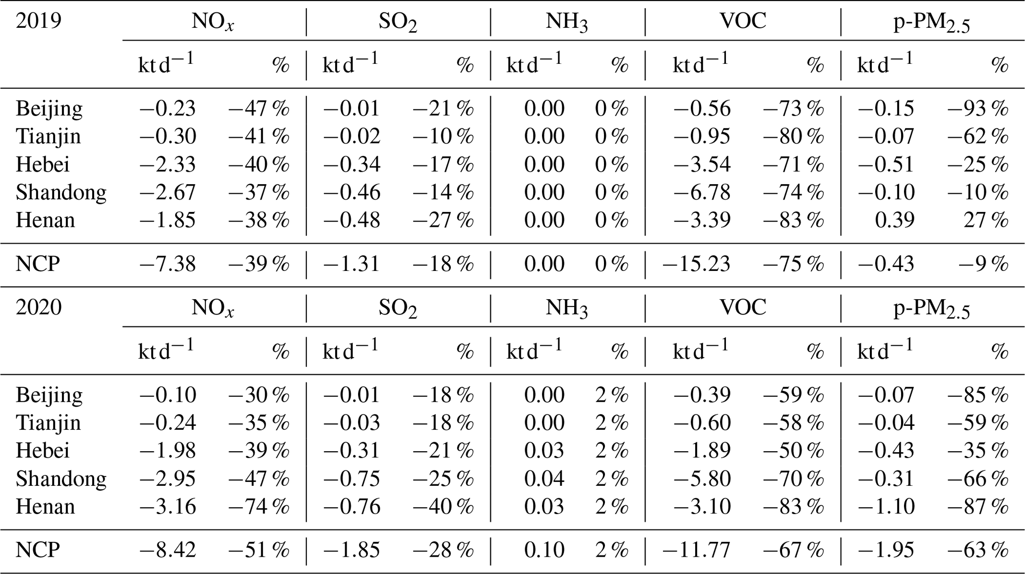
The influence of the shutdown is estimated as the difference in emissions between Period 2H (hypothetical emissions without shutdown effects) and Period 2 (actual emissions), as shown in Fig. 3 (grey and red bars respectively) and detailed in Table 3 by NCP province. Due to the COVID-19 shutdown in 2020, emissions of NOx, VOC and PM2.5 decreased substantially by 51 %, 67 % and 63 %, respectively. SO2 emissions also decreased by 28 %, while NH3 emissions experienced very small increases (+2 %) which might be associated with increased activities in rural areas (e.g., potential NH3 emission sources like stool burning) as many people relocated from megacities to small towns or the countryside. Compared to the effects of the Spring Festival in 2019, the COVID-19 shutdown led to greater reductions in NOx, SO2 and PM2.5 emissions. The smaller VOC reduction in 2020 compared to 2019 might be due to the difference in temporal coverage of Period 2 in the 2 years (i.e., there were more warm days in Period 2 in 2020). Note that the hypothetical emissions in Period 2H are estimated based on the assumption of no shutdown effects in both Period 1 and Period 3. Therefore the reduction of those pollutant emissions in 2020 might be even larger considering the lag effects of COVID-19.
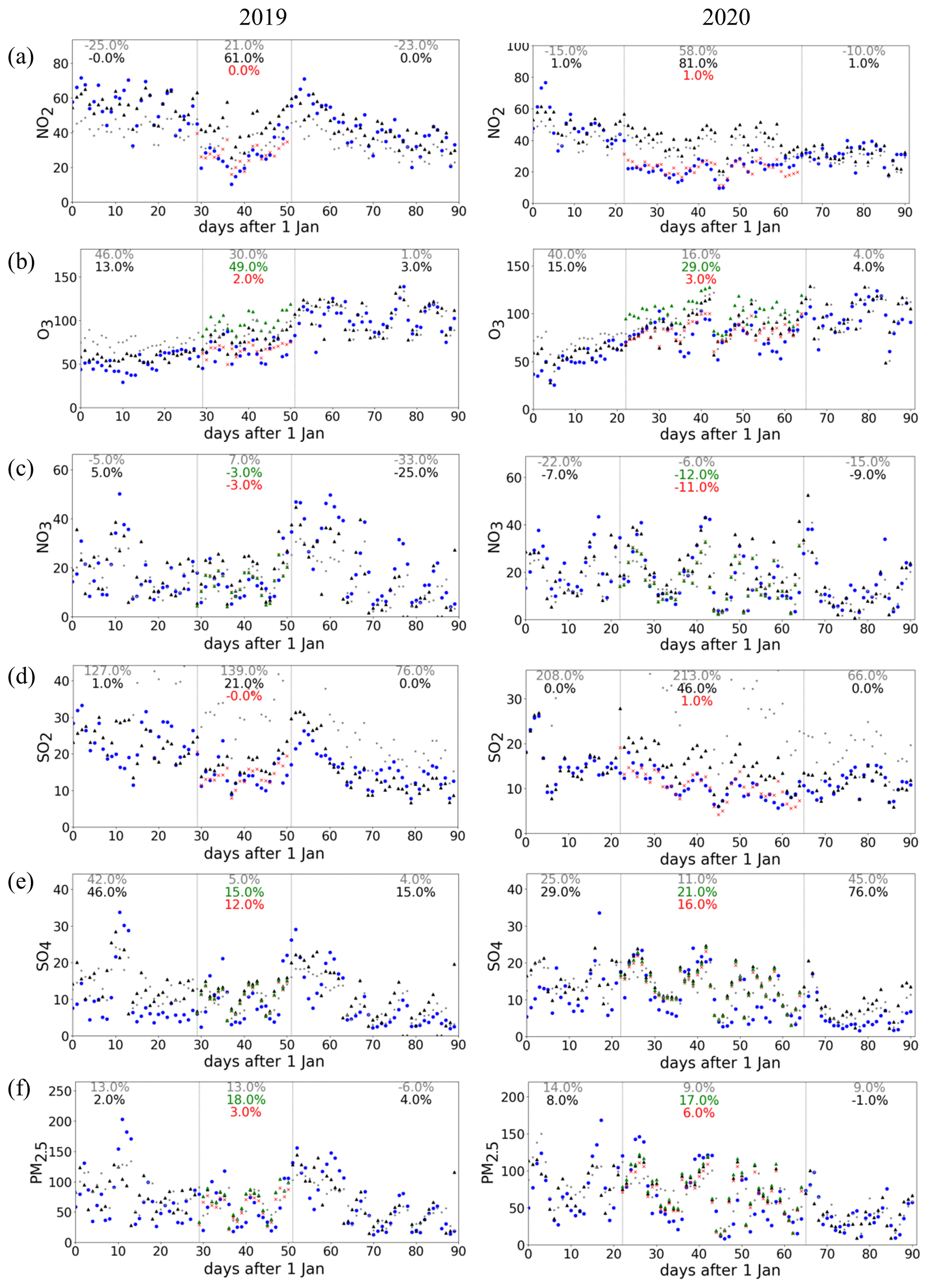
Figure 4Comparison of the simulated and observed average concentrations on the NCP. The percentage numbers indicate the normalized mean biases in hypothesis and actual simulations respectively for Period 2. Blue dots: observations; black dots: simulations using adjusted emission with no consideration of shutdown influences; red dots: simulations using adjusted emission with consideration of shutdown influences; green dots: simulations using adjusted emission with consideration of shutdown influences without VOC for O3, NH3 for , SO2 for , primary PM2.5 for PM2.5; grey dots: original simulations without assimilation; the regional average concentrations were calculated using spatially and temporally matched simulated and observed values; unit: µg m−3.
3.2 The shutdown effects on ambient concentrations
Using the RSM, we predicted concentrations based on the updated emissions from the response-based inversion model. In general, the simulated concentrations based on the adjusted emissions matched well with the observed concentrations, as shown in Fig. 4 for NCP averages and detailed by province in Figs. S1–S12 in the Supplement. More important, during the shutdown period in both years, the simulations using adjusted emissions without considering shutdown influences significantly overestimate the NO2 concentrations in 2019 and 2020 by 61 % and 81 %, respectively. The high biases in 2019 and 2020 are reduced to within 1 % in the simulation with consideration of shutdown effects (Fig. 4a). To evaluate the performance of assimilation, we also conducted the cross validation by using 50 % observation sites for estimating the emission ratio to be applied on the remaining 50 % of observation sites for testing. The performance of cross validation is examined, suggesting quite similar results with that using all observation sites as shown in Fig. 4. The estimated percent changes in emissions due to the shutdown in Period 2 from cross validation are also close to that using all observation sites, as shown in Fig. S13.
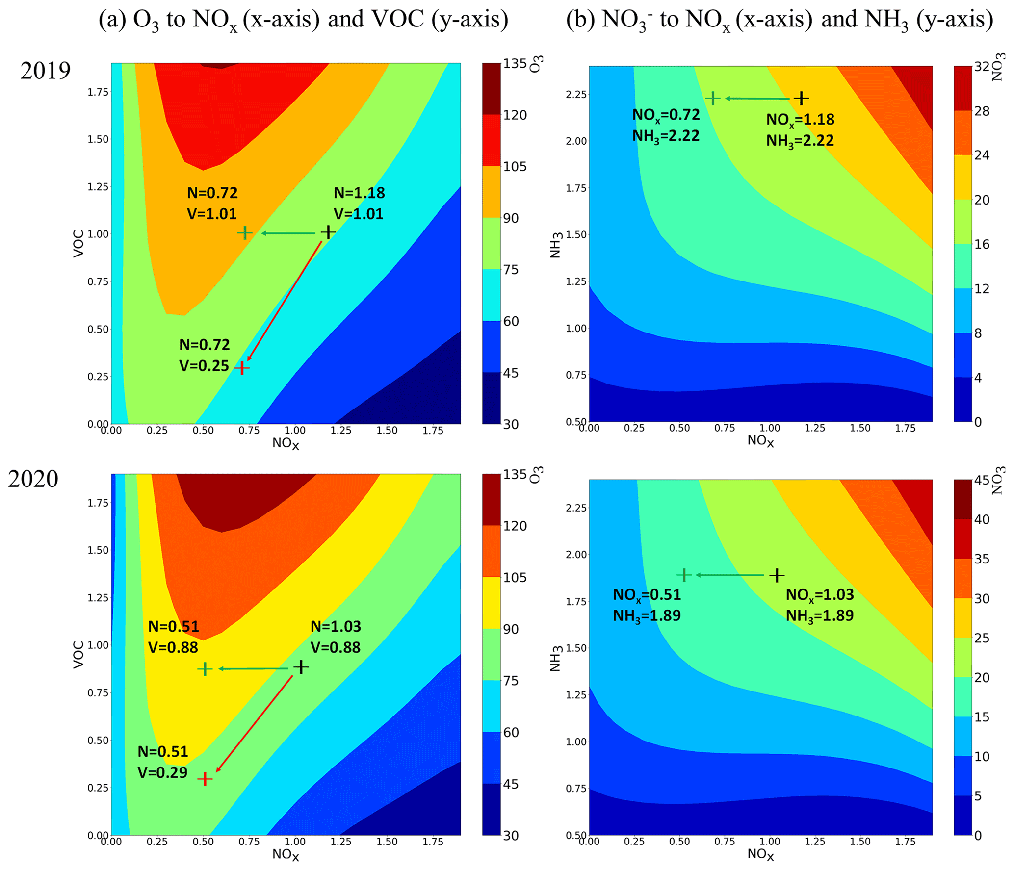
Figure 5Implication of emission changes from the O3 and response isopleths during shutdowns. The axes indicate emission ratios relative to the prior emissions; black symbol: adjusted emission ratios with no consideration of shutdown; red symbol: adjusted emission ratios with consideration of shutdown; green symbol: adjusted emission ratios without considering simultaneous VOC changes for O3, and NH3 changes for NO3; background color: O3 and concentrations, µg m−3.
The results for O3 are quite interesting, as simulated O3 concentrations are close to observations in both simulations with and without consideration of shutdown influences (Fig. 4b). The apparent insensitivity of O3 concentrations to emission changes during the shutdown can be explained by the opposite response of O3 to its two precursors, NOx and VOC. In Fig. 5a, we compare the response of O3 concentrations for two NOx and VOC emission change pathways starting from the hypothetical emissions for no-shutdown conditions (black symbol in Fig. 5a). Since NOx emissions clearly decreased due to the shutdown, the O3 concentrations would increase if VOC emissions remained constant (following the green line to the green symbol in Fig. 5a). Yet the simulation without consideration of VOC emission changes would result in a high bias of simulated O3 concentrations compared to the observations by 49 % in 2019 and 29 % in 2020. The low observed O3 concentrations during Period 2 in both years indicates that VOC emission reductions must have occurred to maintain the suppressed O3 level (following the red line to the red symbol in Fig. 5a). Consistent with this interpretation, the simulated O3 concentrations agree well with observations (e.g., normalized mean bias, NMB <3 %) when both NOx and VOC emission reductions are represented.
The substantial reduction of NOx emissions also resulted in noticeable decreases in concentrations (black and green lines in Fig. 4c). However, the low bias in predictions cannot be readily mitigated by adjusting the NH3 emissions, because the substantial decreases in NOx emissions associated with the shutdown result in strong NH3-rich conditions, where concentrations are less sensitive to NH3 emissions increases. The response of concentrations to pathways of NOx and NH3 emission changes is depicted in Fig. 5b (SO2 and VOC emissions are also changing simultaneously with NOx). A larger decrease in simulated (from that with no consideration of shutdown influences) than observed concentrations is associated with the NOx emission reductions, but the change of NH3 emissions can hardly increase the concentrations under such strong NH3-rich conditions. Therefore, the model predicted no NH3 changes in 2019, but very small increases of NH3 emissions (+2 %) in 2020 due to the increased activities in rural areas, which slightly reduced the low biases (NMB from −12 % to −11 %).
The large reduction in SO2 emissions estimated with the response model during the 2020 shutdown considerably reduced the high biases in simulated SO2 and concentrations (Fig. 4d–f). However, the biases are still considerable after the emission adjustment because a large fraction of might come from primary sources, which need further investigation especially for its contribution to p-PM2.5.
Agreement between the simulated and observed PM2.5 concentrations also improves when accounting for the reductions in primary PM2.5 emissions estimated with the response model in both years (Fig. 4g). Another interesting finding is that the simulated PM2.5 concentrations with consideration of all emission changes due to the shutdown (red line in Fig. 4g) are quite similar to PM2.5 predictions without consideration of the shutdown impacts (black line in Fig. 4g). The same behavior is evident for O3 concentrations (red and black lines in Fig. 4b). As discussed above, the reductions in emissions of multiple species during the shutdown had compensating influences on air quality, and the overall effects of the emission changes on O3 and PM2.5 concentrations were neutralized to a relatively small level.

Figure 6Contributions to the changes of O3 and PM2.5 concentrations during Period 2. OBS: observation; oSIM: no consideration of shutdown; ΔNOx: impacts due to the change of NOx emissions; ΔVOC: impacts due to the change of VOC emissions; ΔNH3: impacts due to the change of NH3 emissions; ΔSO2: impacts due to the change of SO2 emissions; Δp-PM2.5: impacts due to the change of primary PM2.5 emissions.
3.3 Impacts of individual emission changes from the shutdown on O3 and PM2.5 concentrations
To further investigate the individual impacts of emission changes of each pollutant on O3 and PM2.5 concentrations, we conducted a sensitivity analysis by sequentially adding each incremental emission change into the model system and then calculating the associated changes in O3 and PM2.5 concentrations. By incrementally adding the impacts of emission changes of five pollutants (ΔNOx, ΔVOC, ΔNH3, ΔSO2 and Δp-PM2.5), the concentrations change from the original simulation, without consideration of shutdown impacts (noted as oSIM, shown as grey bar in Fig. 6), and ultimately reaching observed levels (noted as OBS, shown as narrow blue bars in Fig. 6). One thing that should be noted is that we scaled the individual impact of emission changes based on the ratio of observation to the adjusted simulation after considering overall impacts, to eliminate the small discrepancy between the observations and the adjusted simulations after considering the overall impacts. Therefore, the overall changes in concentrations due to the shutdown can be reflected by the difference between the observation (OBS) and simulation with no consideration of shutdown (oSIM).
For O3, the reduction of NOx emissions leads to a significant enhancement of O3 (see ΔNOx) due to the VOC-limited regime in winter (Xing et al., 2019), while such an O3 enhancement has been largely or completely mitigated thanks to the simultaneous reduction of VOC emissions (see ΔVOC) in both 2019 and 2020. This behavior is particularly evident in Henan and Shandong provinces, which experienced substantial VOC reductions during the shutdown (Table 3). Such benefits from simultaneous VOC controls also occurred for PM2.5 concentrations. Compared with O3, the changes in PM2.5 concentrations are more complex to interpret due to the influence of emission changes for SO2 (ΔSO2), NH3 (ΔNH3) and p-PM2.5 (Δp-PM2.5) in addition to NOx and VOC. Results suggest that the reductions of p-PM2.5 emissions tended to favor PM2.5 decreases, while the ΔSO2 and ΔNH3 emission changes have negligible influence. Overall, reductions in p-PM2.5 and VOC emissions helped mitigate potential PM2.5 concentration enhancements in most NCP provinces. Similar findings are suggested in Hang et al. (2020), who observed enhanced secondary pollution during the COVID-19 period. The air quality impacts from the unexpected controls during the COVID-19 shutdown suggest that strengthened controls on p-PM2.5 emissions and well-balanced reductions in NOx and VOC emissions would be an effective strategy for further improving air quality on the NCP (Xing et al., 2018).
In summary, this study developed a response-based inversion modeling framework and applied it to characterize the emission changes and associated air quality impacts during the 2019 Spring Festival and the 2020 COVID-19 pandemic shutdown. Our results indicate that the response model can effectively adjust the assumed prior emissions such that air quality predictions match well with observed concentrations. The model also captures the temporal variations of emissions associated with changes in meteorological conditions. The model may suffer some uncertainties from deficiencies in model chemical mechanisms (e.g., conversion of SO2 to ), as well as the quality of prior emissions and limited coverage of observations. Difficulties are also found in estimating the NH3 emission changes under strong NH3-rich conditions by using the current inversion method based on the concentration of PM chemical components. However, with the continued growth in observational datasets from both surface monitors and satellite retrievals, improvements in knowledge of atmospheric science and development of advanced assimilation technologies, the new response-based inversion model has great potential to further improve the accuracy and efficiency of emission inventory updates. The importance of reliable bottom-up inventories for defining prior emissions by sector, combined with the ability of the top-down inversion model to rapidly adjust emissions for consistency with observations, demonstrates how bottom-up and top-down emissions modeling methods are complementary.
The response model was applied to the investigation of emission changes during the COVID-19 shutdown. The emission changes were estimated by comparing emissions for actual conditions with emissions for hypothetical conditions assuming that the shutdown did not occur. Emission levels during the COVID-19 shutdown period were estimated by applying the temporal profiles of sectoral emissions from the bottom-up inventory. These estimates may suffer some uncertainties associated with the temporal profiles and the assumption of no shutdown impacts during the post-shutdown period. Our results suggest that the shutdowns in 2019 and 2020 had considerable impacts on air pollutant emissions. Longer and stronger impacts are found in 2020 due to the COVID-19 pandemic compared to the Spring Festival of the previous year. The anthropogenic emissions of NO2, SO2, VOC and primary PM2.5 on the NCP were reduced by 51 %, 28 %, 67 % and 63 %, respectively, due to the COVID-19 shutdown in 2020. The estimated ratio might be slightly underestimated considering the lag effects after the COVID-19 shutdown. We also found that emission changes associated with the shutdown periods had limited impacts on surface O3 and PM2.5 concentrations due to compensating effects of emission changes in different pollutants. Based on our analysis, careful controls on NOx emission sources on the NCP are recommended in combination with simultaneous controls on VOC and NH3 sources. Such a comprehensive strategy would minimize the potential negative impacts on air quality of NOx emission reductions during VOC-limited conditions in winter. This study also illustrates that air quality improvements do not necessary follow from precursor emission reductions, and multi-pollutant nonlinear response models are therefore critical tools for representing the nonlinear relationship between emissions and concentrations in designing effective control strategies.
The original data and code used in this study are available upon request from the corresponding authors.
The supplement related to this article is available online at: https://doi.org/10.5194/acp-20-14347-2020-supplement.
JX and SL designed the methodology, conducted the analysis and wrote the original draft. YJ conducted the WRF-CMAQ simulation. SW, DD, ZD and JH helped with the bottom-up emission inventory. YZ helped with the RSM model. All authors contributed to writing the paper.
The authors declare that they have no conflict of interest.
This work was completed on the “Explorer 100” cluster system of Tsinghua National Laboratory for Information Science and Technology. We thank Carey Jang, James Kelly, Jian Gao and Jingnan Hu for contributions to the study. The authors gratefully acknowledge the free availability and use of observation datasets.
This research has been supported by the National Key R & D program of China (grant no. 2018YFC0213805) and the National Natural Science Foundation of China (grant nos. 21625701 and 41907190).
This paper was edited by Tim Butler and reviewed by two anonymous referees.
Cao, H., Fu, T.-M., Zhang, L., Henze, D. K., Miller, C. C., Lerot, C., Abad, G. G., De Smedt, I., Zhang, Q., van Roozendael, M., Hendrick, F., Chance, K., Li, J., Zheng, J., and Zhao, Y.: Adjoint inversion of Chinese non-methane volatile organic compound emissions using space-based observations of formaldehyde and glyoxal, Atmos. Chem. Phys., 18, 15017–15046, https://doi.org/10.5194/acp-18-15017-2018, 2018.
Ding, D., Xing, J., Wang, S., Liu, K., and Hao, J.: Estimated contributions of emissions controls, meteorological factors, population growth, and changes in baseline mortality to reductions in ambient PM2.5 and PM2.5-related mortality in China, 2013–2017, Environ. Health Persp., 127, 067009, https://doi.org/10.1289/EHP4157, 2019.
Hartley, D. and Prinn, R.: Feasibility of determining surface emissions of trace gases using an inverse method in a three-dimensional chemical transport model, J. Geophys. Res.-Atmos., 98, 5183–5197, 1993.
Huang, X., Ding, A., Gao, J., Zheng, B., Zhou, D., Qi, X., Tang, R., Wang, J., Ren, C., Nie, W., Chi, X., Xu, Z., Chen, L., Li, Y., Che, F., Pan, N., Wang, H., Tong, D., Qin, W., Cheng, W., Liu, W., Fu, Q., Liu, B., Chai, F., Davis, S. J., Zhang, Q., and He, K.: Enhanced secondary pollution offset reduction of primary emissions during covid-19 lockdown in china, National Science Review, nwaa137, https://doi.org/10.1093/nsr/nwaa137, 2020.
Li, L., Li, Q., Huang, L., Wang, Q., Zhu, A., Xu, J., Liu, Z., Li, H., Shi, L., Li, R., and Azari, M.: Air quality changes during the COVID-19 lockdown over the Yangtze River Delta Region: An insight into the impact of human activity pattern changes on air pollution variation, Sci. Total Environ., 732, 139282 https://doi.org/10.1016/j.scitotenv.2020.139282, 2020.
Li, M., Zhang, Q., Kurokawa, J.-I., Woo, J.-H., He, K., Lu, Z., Ohara, T., Song, Y., Streets, D. G., Carmichael, G. R., Cheng, Y., Hong, C., Huo, H., Jiang, X., Kang, S., Liu, F., Su, H., and Zheng, B.: MIX: a mosaic Asian anthropogenic emission inventory under the international collaboration framework of the MICS-Asia and HTAP, Atmos. Chem. Phys., 17, 935–963, https://doi.org/10.5194/acp-17-935-2017, 2017.
Lu, Z., Streets, D. G., de Foy, B., Lamsal, L. N., Duncan, B. N., and Xing, J.: Emissions of nitrogen oxides from US urban areas: estimation from Ozone Monitoring Instrument retrievals for 2005–2014, Atmos. Chem. Phys., 15, 10367–10383, https://doi.org/10.5194/acp-15-10367-2015, 2015.
Mendoza-Dominguez, A. and Russell, A. G.: Iterative inverse modeling and direct sensitivity analysis of a photochemical air quality model, Environ. Sci. Technol,, 34, 4974–4981, 2000.
Miyazaki, K., Eskes, H., Sudo, K., Boersma, K. F., Bowman, K., and Kanaya, Y.: Decadal changes in global surface NOx emissions from multi-constituent satellite data assimilation, Atmos. Chem. Phys., 17, 807–837, https://doi.org/10.5194/acp-17-807-2017, 2017.
Napelenok, S. L., Pinder, R. W., Gilliland, A. B., and Martin, R. V.: A method for evaluating spatially-resolved NOx emissions using Kalman filter inversion, direct sensitivities, and space-based NO2 observations, Atmos. Chem. Phys., 8, 5603–5614, https://doi.org/10.5194/acp-8-5603-2008, 2008.
Shi, X. and Brasseur, G. P.: The Response in Air Quality to the Reduction of Chinese Economic Activities during the COVID-19 Outbreak, Geophys. Res. Lett., 47, e2020GL088070, https://doi.org/10.1029/2020GL088070, 2020.
Tang, W., Cohan, D. S., Lamsal, L. N., Xiao, X., and Zhou, W.: Inverse modeling of Texas NOx emissions using space-based and ground-based NO2 observations, Atmos. Chem. Phys., 13, 11005–11018, https://doi.org/10.5194/acp-13-11005-2013, 2013.
Tang, W., Arellano, A. F., Gaubert, B., Miyazaki, K., and Worden, H. M.: Satellite data reveal a common combustion emission pathway for major cities in China, Atmos. Chem. Phys., 19, 4269–4288, https://doi.org/10.5194/acp-19-4269-2019, 2019.
Wang, P., Chen, K., Zhu, S., Wang, P., and Zhang, H.: Severe air pollution events not avoided by reduced anthropogenic activities during COVID-19 outbreak, Resour. Conserv. Recy., 158, 104814, https://doi.org/10.1016/j.resconrec.2020.104814, 2020.
Wang, Q. and Su, M.: A preliminary assessment of the impact of COVID-19 on environment – A case study of China, Sci. Total Environ., 728, 138915, https://doi.org/10.1016/j.scitotenv.2020.138915, 2020.
Wang, S., Zhao, M., Xing, J., Wu, Y., Zhou, Y., Lei, Y., He, K., Fu, L., and Hao, J.: Quantifying the air pollutants emission reduction during the 2008 Olympic Games in Beijing, Environ. Sci. Technol., 44, 2490–2496, 2010.
Wang, S., Xing, J., Chatani, S., Hao, J., Klimont, Z., Cofala, J., and Amann, M.: Verification of anthropogenic emissions of China by satellite and ground observations, Atmos. Environ., 45, 6347–6358, 2011a.
Wang, S., Xing, J., Jang, C., Zhu, Y., Fu, J. S., and Hao, J.: Impact assessment of ammonia emissions on inorganic aerosols in East China using response surface modeling technique, Environ. Sci. Technol., 45, 9293–9300, 2011b.
Xing, J., Wang, S. X., Jang, C., Zhu, Y., and Hao, J. M.: Nonlinear response of ozone to precursor emission changes in China: a modeling study using response surface methodology, Atmos. Chem. Phys., 11, 5027–5044, https://doi.org/10.5194/acp-11-5027-2011, 2011.
Xing, J., Pleim, J., Mathur, R., Pouliot, G., Hogrefe, C., Gan, C.-M., and Wei, C.: Historical gaseous and primary aerosol emissions in the United States from 1990 to 2010, Atmos. Chem. Phys., 13, 7531–7549, https://doi.org/10.5194/acp-13-7531-2013, 2013.
Xing, J., Wang, S., Zhao, B., Wu, W., Ding, D., Jang, C., Zhu, Y., Chang, X., Wang, J., Zhang, F., and Hao, J.: Quantifying nonlinear multiregional contributions to ozone and fine particles using an updated response surface modeling technique, Environ. Sci. Technol., 51, 11788–11798, 2017.
Xing, J., Ding, D., Wang, S., Zhao, B., Jang, C., Wu, W., Zhang, F., Zhu, Y., and Hao, J.: Quantification of the enhanced effectiveness of NOx control from simultaneous reductions of VOC and NH3 for reducing air pollution in the Beijing–Tianjin–Hebei region, China, Atmos. Chem. Phys., 18, 7799–7814, https://doi.org/10.5194/acp-18-7799-2018, 2018.
Xing, J., Ding, D., Wang, S., Dong, Z., Kelly, J. T., Jang, C., Zhu, Y., and Hao, J.: Development and application of observable response indicators for design of an effective ozone and fine-particle pollution control strategy in China, Atmos. Chem. Phys., 19, 13627–13646, https://doi.org/10.5194/acp-19-13627-2019, 2019.
Xing, J., Li, S., Ding, D., Kelly, J.T., Wang, S., Jang, C., Zhu, Y., and Hao, J. M.: Data assimilation of ambient concentrations of multiple air pollutants using an emission-concentration response modeling framework, Atmosphere, in press, 2020a.
Xing, J., Zheng, S., Ding, D., Kelly, J. T., Wang, S., Li, S., Qin, T., Ma, M., Dong, Z., Jang, C., and Zhu, Y.: Deep learning for prediction of the air quality response to emission changes, Environ. Sci. Technol., 54, 8589–8600, 2020b.
Zhang, L., Chen, Y., Zhao, Y., Henze, D. K., Zhu, L., Song, Y., Paulot, F., Liu, X., Pan, Y., Lin, Y., and Huang, B.: Agricultural ammonia emissions in China: reconciling bottom-up and top-down estimates, Atmos. Chem. Phys., 18, 339–355, https://doi.org/10.5194/acp-18-339-2018, 2018.
Zhang, S., Xing, J., Sarwar, G., Ge, Y., He, H., Duan, F., Zhao, Y., He, K., Zhu, L., and Chu, B.: Parameterization of heterogeneous reaction of SO2 to sulfate on dust with coexistence of NH3 and NO2 under different humidity conditions, Atmos. Environ., 208, 133–140, 2019.