Total column ozone in New Zealand and in the UK in the 1950s

Total column ozone measurements reach back almost a century. Historical column ozone data are important not only for obtaining a long-term perspective of changes of the ozone layer but arguably also as diagnostics of lower-stratospheric or tropopause-level flow in time periods of sparse upper-air observations. With the exception of a few high-quality records such as that from Arosa, Switzerland, ozone science has almost exclusively focused on data since the International Geophysical Year (IGY) in 1957–1958, although earlier series exist. In the early 2000s, we digitised and re-evaluated many pre-IGY series. Here we add a series from Wellington, New Zealand, from 1951 to 1959. We re-evaluated the data from the original observation sheets and performed quality control analysis, and here we present the data. The day-to-day variability can be used to assess the quality of reanalysis products, since the data cover a region and time period with only few upper-air data. Comparison with total column ozone in the reanalyses ERA-PreSAT (which assimilates upper-air data) and 20CRv3 and CERA-20C (which do not assimilate upper-air data) shows high correlations with all three. Although trend quality is doubtful (no calibration information and no intercomparisons are available), combining the record with other available data (including historical data from Australian locations) allows a 70-year perspective of ozone changes over the southern mid-latitudes. The series will be available from the World Ozone and Ultraviolet Data Centre. Finally, we also present a short series from Downham Market, UK, covering November 1950 to October 1951, and publish it with further historical data series that were previously described but not published.

1 Introduction

Regular total column ozone measurements reach back almost a century (Fabry and Buisson, 1921; Dobson and Harrison, 1926). While interest first arose from its close relation to tropopause flow, which seemed promising as a meteorological diagnostic prior to the invention of the radiosonde, the focus then shifted towards understanding stratospheric circulation and monitoring of the ozone layer. Historical data were not considered particularly important until the onset of ozone depletion and the discovery of the Antarctic ozone hole. Even then, the focus was on ozone changes since the International Geophysical Year (IGY) in 1957–1958, when a global network was initiated and a new measurement protocol (double-wavelength pair) was introduced, leading to higher-quality measurements (Dobson, 1957a, b; Dobson and Normand, 1957). Only a few of the longer records were re-evaluated, such as those from Arosa (Staehelin et al., 1998), Tromsø (Hansen and Svenøe, 2005), and Oxford (Vogler et al., 2007). These records provide an important basis for trend assessments (see also Müller, 2009, and Bojkov, 2012, for a history of ozone measurements).

In the early 2000s, the first author compiled and digitised a considerable number of pre-IGY series in order to exploit their relation to tropopause flow and the stratospheric meridional circulation (Brönnimann et al., 2003a, b). Trend quality is not necessarily required for such applications since the day-to-day variation at mid-latitudes is much larger than the trend. The data were digitised and homogenised if possible, and some (but not all) were delivered to the World Ozone and Ultraviolet Data Centre (WOUDC). Not all existing series could be found however. Here we add further series to this collection, namely from Wellington, New Zealand, from 1951 to 1959 (the data from the IGY onward are already in the WOUDC database) and a short and patchy series from Downham Market, UK, from November 1950 to October 1951. In this paper we present the series and their quality control and show selected analyses. The data are used to independently assess reanalysis data sets, and the long-term changes of ozone over the southern mid-latitudes since the 1950s is presented.

The paper is organised as follows. Section 2 presents the instrument history and Sect. 3 describes the data re-evaluation. Comparisons with upper-air data and reanalysis data sets are presented in Sect. 4. In Sect. 5 we provide an assessment of the data quality and compare the results with the literature. Conclusions are drawn in Sect. 6.

2 Ozone data and instrument histories

2.1 Wellington

Already during Dobson's first (photographic) global ozone network in the late 1920s (Dobson et al., 1930), New Zealand participated by hosting a spectrophotometer in Christchurch (Fig. 1). When Dobson built the new photoelectric instruments in the 1930s (Dobson, 1931) and planned a global network with these instruments, New Zealand was approached again and in 1937 eventually placed an order (see Nichol, 2018; Farkas, 1954). However, delays occurred, and the designated instrument (Dobson Instrument No. 17, in short D#17) was only finished shortly before the war. When the war started, the UK approached New Zealand and asked to withhold the delivery of D#17 in order to use it in the UK. The instrument operated in the UK until 1947. It was then decided that a recalibration and improvement was necessary before the instrument could be shipped to New Zealand; therefore, the instrument was sent to Oxford. The photoelectric cell and amplifier were replaced by a photomultiplier (Farkas, 1954). In Dobson's original observation sheets from Oxford (Vogler et al., 2007) we found measurements performed with D#17 on 24 February and 1 March 1940 and then again on 21 and 22 November 1946. This was presumably before the upgrade. Note, however, that these observation sheets are incomplete. No sheets from Oxford could be found for the period from January 1947 to October 1949, which might have contained the calibration information (together with other measurements from Oxford, which are lost).

Figure 1 Map of the stations used (circles: ozone; triangles: upper air).

The instrument was sent from the UK only in late 1949 and arrived in New Zealand in 1950. The instrument was first tested, and it was found that the settings of the quartz plates had changed during the transport (Farkas, 1954). As a consequence, a new table of plate settings was produced for operations. Then the instrument was put in operation in Kelburn, Wellington (41.28^∘ S, 174.77^∘ E, Fig. 1).

The first measurements are dated 1 August 1951. In the first years, Elizabeth Porter was in charge of the measurements. After her unexpected death in 1953, Edith Farkas took over and was in charge of operations until the mid-1980s. The instrument underwent another major rehaul in 1963–1964. On this occasion it was also compared with D#105 (Nichol, 2018).

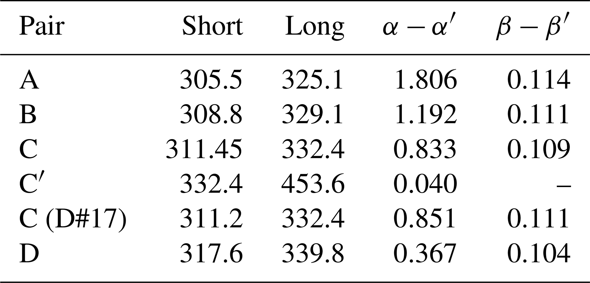
For all observations, the shorter wavelength was 311.2 nm (C pair; see Table 1), and measurements were taken in direct-sun (DS) mode as well as at the blue (ZB) or cloudy zenith (ZC, using an additional wavelength that is not strongly absorbed by ozone; the pair formed by the two longer wavelengths, sometimes termed C^′, allows addressing the attenuation by clouds; see Table 1). The relative path length through the ozone layer, μ, was calculated from a nomogram. The altitude of the ozone layer was assumed to be 22 km. For DS measurements, an atmospheric correction was added, which was assumed to be 0.095 m atm cm for clear days, 0.1 m atm cm for slightly hazy days, and more (usually 0.11 m atm cm) for very hazy days.

Table 1 Wavelengths (nm) and absorption and scattering coefficients for different wavelength pairs for standard settings (Komhyr et al., 1993; Komhyr and Evans, 2008) and for the instrument in Kelburn.

Observations at the blue or cloudy zenith require calibration using quasi-simultaneous observations. In 1954, when the report was published, only a limited set of such observations was available; values were described as somewhat doubtful (Farkas, 1954). For this paper, we thus recalibrated these measurements.

Farkas (1992) and Nichol (2018) consider the data prior to 1964 unreliable, as no intercomparison had been made. For the sake of completeness, Nichol (2018) shows data from the IGY onward, though noting their inferior quality. These data, from July 1957 onward, are available from the WOUDC. However, the data prior to 1957 have so far not been available electronically. The earliest data were published by Farkas (1954), where in addition to the reduced ozone amount the observation mode, wavelength pair used, and observation time were also indicated. Reduced values were sent to the International Ozone Commission, where the communication was stored and later sent to Environment Canada. It was scanned and recently sent to the first author as a PDF file comprising 1527 pages (Alkis Bais, personal communication, 2016). The title of the folder is “Early Total Ozone Information”, and a data range on the title page is given as 1959–1964; it nevertheless contains a number of earlier series, among them the Wellington and Downham Market data.

We digitised the total column ozone data from both sources: the PDF file from the International Ozone Commission and Farkas (1954). Upon inquiry, the original data sheets (covering 1951 to 1960) were found at NIWA (National Institute for Water and Atmospheric Research), scanned, and sent to the first author (Fig. 2). The original readings were then also digitised. The main source of information in this paper is the original sheets; the reduced values from the other two sources were used for cross-checking. Note that we do not have calibration information or intercomparison data. However, the data sheets contain many notes that provide additional information on the instrument history. This information will be given in Sect. 3.

Figure 2 Original data sheet from Wellington, NZ.

2.2 Downham Market

The scans from the International Ozone Commission also contained data from Downham Market (52.61^∘ N, 0.38^∘ E), though they are almost illegible. These are daily averaged reduced total column measurements with no additional information. They covered the year 1951 (January to October). We supplemented these data with values printed on a graph (incidentally, this was a New Year's card sent out by the International Ozone Commission, Fig. 3), such that we could extend the series backward to late November 1950. Note that both sources of information are secondary sources and thus inherently unreliable. Nevertheless, as will be shown, the quality of the data seems unexpectedly high.

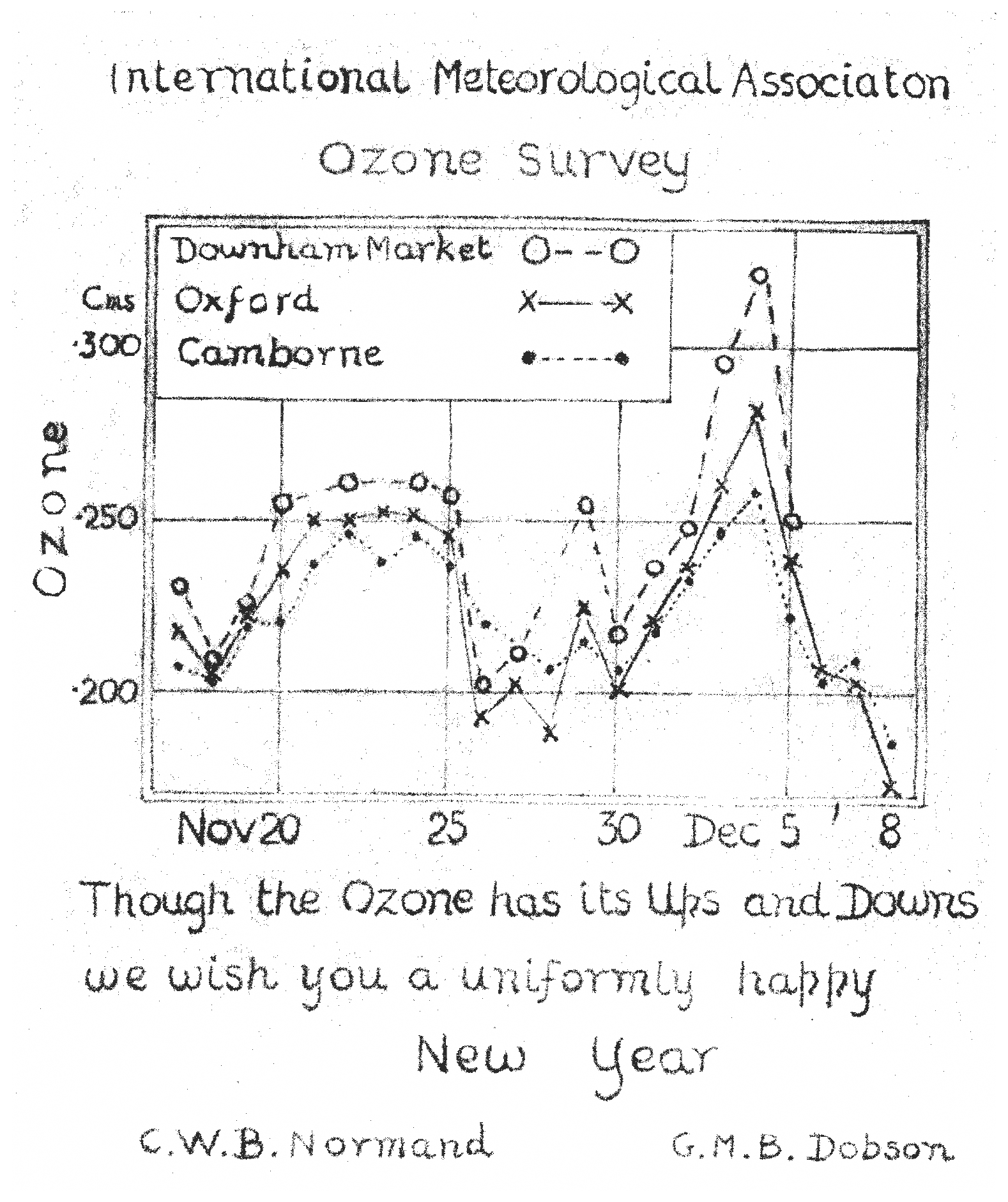
Figure 3 New Year's card with data from Downham Market, 1950.

Sometimes monthly means were indicated on the sheet, which we could use to cross-check our digitisation. Additionally, monthly data from Downham Market (November 1950 to October 1951) were found in the communication of the International Ozone Commission, stored at the UK Met Office (Normand, 1961). Photocopies of this archive folder were sent to the first author by Stephen Farmer (UK Met Office) in 2000. There is a large overlap between this file and the PDF file from Environment Canada, but there are also unique data in each of the folders. These data were also used to cross-check where there were no monthly means in the other source, although there were also sometimes differences between the monthly means from both sources. This second source (Normand, 1961) also showed us that the record would have continued into November 1951 for at least 17 d, and that 15 and 26 daily values are missing from our source for November and December 1950, respectively.

Nothing is known about the instrument or the history of the measurements. We assume that the instrument (the number remains unknown) was relocated to Hemsby in November 1951. Brönnimann et al. (2003b) digitised the Hemsby total column ozone data and found them to be of good quality (in terms of day-to-day changes) apart from an implausible (flagged) period. The context of the measurements also remains unknown. Scrase (1951) mentions the testing of radiosondes at Downham Market in approximately the same period.

3 Re-evaluation and analysis methods

3.1 General procedure

The processing of Dobson data is described in Komhyr and Evans (2008); the standard procedure to re-evaluate the data is given in Bojkov et al. (1993). We followed the two guidelines as closely as possible. Note, however, that no calibration information and no intercomparison data were available. The standard equation for calculating total column ozone X (in atmosphere centimetres at standard pressure) from a single-wavelength pair (with short and long wavelengths: λ and λ^′, respectively) is

$$\begin{array}{}\text{(1)}& X={\displaystyle \frac{N-\left(\mathit{\beta }-{\mathit{\beta }}^{\prime }\right)\frac{mp}{p_{\mathrm{0}}}-\left(\mathit{\delta }-{\mathit{\delta }}^{\prime }\right)\sec \left(\mathrm{SZA}\right)}{\left(\mathit{\alpha }-{\mathit{\alpha }}^{\prime }\right)\mathit{\mu }}},\end{array}$$

where β is the molecular scattering coefficient (primes denote the longer wavelength), α is the absorption coefficient, δ is the aerosol scattering coefficient, m is the relative air mass, μ is the relative path length through the ozone layer, SZA is the solar zenith angle, and p and p₀ are station and mean-sea-level pressure. The relative intensity N is the actual measurement:

$$\begin{array}{}\text{(2)}& N=\log \left({\displaystyle \frac{I_{\mathrm{0}}}{I_{\mathrm{0}}^{\prime }}}\right)-\log \left({\displaystyle \frac{I}{I^{\prime }}}\right),\end{array}$$

where I and I₀ are the intensities at the surface and outside the Earth's atmosphere, respectively. N is obtained from the dial reading at the instrument, R, via a conversion table (R−N table). No unique value can be given for the aerosol scattering coefficient ($\mathit{\delta }-{\mathit{\delta }}^{\prime }$) as it depends on the haziness of the atmosphere.

For double-wavelength pairs such as AD or BD, the following equation is used:

$$\begin{array}{}\text{(3)}& \begin{array}{rl}{X}_{\mathrm{12}}& ={\displaystyle \frac{\left(N_{\mathrm{1}}-N_{\mathrm{2}}\right)-\left[{\left(\mathit{\beta }-{\mathit{\beta }}^{\prime }\right)}_{\mathrm{1}}-{\left(\mathit{\beta }-{\mathit{\beta }}^{\prime }\right)}_{\mathrm{2}}\right]\frac{mp}{p_{\mathrm{0}}}}{\left[{\left(\mathit{\alpha }-{\mathit{\alpha }}^{\prime }\right)}_{\mathrm{1}}-{\left(\mathit{\alpha }-{\mathit{\alpha }}^{\prime }\right)}_{\mathrm{2}}\right]\mathit{\mu }}}\\ & -{\displaystyle \frac{\left[{\left(\mathit{\delta }-{\mathit{\delta }}^{\prime }\right)}_{\mathrm{1}}-{\left(\mathit{\delta }-{\mathit{\delta }}^{\prime }\right)}_{\mathrm{2}}\right]\sec \left(\mathrm{SZA}\right)}{\left[{\left(\mathit{\alpha }-{\mathit{\alpha }}^{\prime }\right)}_{\mathrm{1}}-{\left(\mathit{\alpha }-{\mathit{\alpha }}^{\prime }\right)}_{\mathrm{2}}\right]\mathit{\mu }}}.\end{array}\end{array}$$

Aerosol scattering can then be neglected, and the equation reduces to

$$\begin{array}{}\text{(4)}& X_{\mathrm{12}}={\displaystyle \frac{\left(N_{\mathrm{1}}-N_{\mathrm{2}}\right)-\left[{\left(\mathit{\beta }-{\mathit{\beta }}^{\prime }\right)}_{\mathrm{1}}-{\left(\mathit{\beta }-{\mathit{\beta }}^{\prime }\right)}_{\mathrm{2}}\right]\frac{mp}{p_{\mathrm{0}}}}{\left[{\left(\mathit{\alpha }-{\mathit{\alpha }}^{\prime }\right)}_{\mathrm{1}}-{\left(\mathit{\alpha }-{\mathit{\alpha }}^{\prime }\right)}_{\mathrm{2}}\right]\mathit{\mu }}}.\end{array}$$

When re-evaluating historical data, the procedure is to first process the DS data (the double-pair data can be processed directly, while the single-pair data require assumptions concerning aerosol scattering). The ZB observations are then calibrated against quasi-simultaneous (typically within minutes) DS observations by fitting N and μ using third-order polynomials (Vanicek et al., 2003):

$$\begin{array}{}\text{(5)}& \begin{array}{rl}X& =c_{\mathrm{0}}+c_{\mathrm{1}}N+c_{\mathrm{2}}\mathit{\mu }+c_{\mathrm{3}}{N}^{\mathrm{2}}+c_{\mathrm{4}}{\mathit{\mu }}^{\mathrm{2}}+c_{\mathrm{5}}{N}^{\mathrm{3}}+c_{\mathrm{6}}{\mathit{\mu }}^{\mathrm{3}}\\ & +c_{\mathrm{7}}N\mathit{\mu }+c_{\mathrm{8}}N{\mathit{\mu }}^{\mathrm{2}}+c_{\mathrm{9}}{N}^{\mathrm{2}}\mathit{\mu }.\end{array}\end{array}$$

Vanicek et al. (2003) recommend splitting the data into seasons and fitting polynomial functions separately.

In a second step, ZC observations are processed. This is done by adjusting N by adding a term ΔN in such a way that they can be processed similarly to ZB observations. For the C pair, ΔN is determined by means of an additional wavelength pair, C^′, the shorter wavelength of which corresponds to the longer wavelength of the C pair. Both wavelengths of the C^′ pair are very little absorbed by ozone and thus allow assessing the aerosol and cloud scattering. The correction additionally depends on the cloud type and altitude. Vanicek et al. (2003) use cloud attenuation tables for the correction; constructing such a table however requires a lot of parallel measurements. Vogler et al. (2006) uses linear regressions of the form

$$\begin{array}{}\text{(6)}& \mathrm{\Delta }N=c_{\mathrm{0}}+c_{\mathrm{1}}{N}_{{\mathrm{C}}^{\prime }}\end{array}$$

separately for situations with high clouds and situations with middle or low clouds. Here, ΔN is the difference between N of a quasi-simultaneous ZB measurement and N of the ZC measurement (both for the C pair), while $N_{{\mathrm{C}}^{\prime }}$ refers to the C^′ pair of the ZC measurement.

If original observations sheets are not available, all that can be used are the calculated total column ozone values as well as, if available, the time of day (which allows calculating SZA). Changes in the absorption scale can be corrected by scaling the data (see Brönnimann et al., 2003b), and statistical corrections must be used otherwise. Assessing the dependence of, for example, differences to a neighbouring station on SZA or on the annual cycle can give some hints on possible causes for biases. Statistical corrections can be made dependent on the seasonal cycle or SZA, although series processed in this way are likely to be of lower quality.

In this paper we followed the former, detailed approach for Wellington and the latter approach for Downham Market. The following sections describe the details of the processing.

3.2 Wellington

All observations, 2500 in total, were digitised. Zenith observations were noted on the sheets, but the distinction between ZB and ZC is not made on the sheets until 1954 (however, prior to that time the observations and calculations indicate whether a zenith observations was performed at the clear or cloudy zenith, and some of the measurements could be double-checked with Farkas, 1954). ZC observations were performed from the beginning, often in pairs (ZB and DS, ZC and DS). Observation pairs of ZB–ZC or observation triplets only follow later. From 1955 onward, there are occasional observations of the A pair, and from 1957 on of the AD pair. In 1957 numerous quasi-simultaneous observations of AD and C pairs were performed; then AD measurements were no longer performed, while BD measurements became frequent.

There are almost no measurements from July 1956 to February 1957, which is also confirmed in the data from the International Ozone Commission. The second half of 1958 was missing entirely from the data sheets, but in that case daily data were sent to the International Ozone Commission and are today found at WOUDC, indicating that data sheets have been lost. Our material continues in January 1959. From September 1959 onward, various problems seem to have occurred, according to notes on the observation sheets. One note reads: “While putting lid back after battery change on 8 October 1959, the quartz plates must have moved. From standard lamp readings the estimated correction for dial readings is as follows: b+9, $c+c^{\prime }+\mathrm{6}$, d+10”. Another note in October 1959 speculated that “Quartz plates might have moved at beginning of September on one of the occasions when silica gel was changed”. From October 1959 onward, data sheets become relatively messy, with black ink, red pencil, and many strike-throughs. It is hard to follow if and which corrections were done. A deterioration was also found in terms of correlation and was visually apparent when plotting the data. Problems with the quartz plates are also mentioned later on (e.g. an adjustment in February 1960 is mentioned). We therefore only consider data prior to September 1959.

From the original observations we basically used only the dial readings R and the time of observations as well as information on the haziness and cloud cover, but all other calculations were nevertheless digitised and provided important information. For instance, we checked the averaging of the different R readings, reassessed the R–N conversion (which is a linear function per wavelength), and found that the relation has not changed over the period under study. In this way we checked all steps of the original calculations where possible. Inconsistencies led to the correction of digitisation errors, of typos on the original sheets, or of miscalculations; however, some could not be resolved and led to the flagging of observations.

From the time we calculated the SZA using the MICA (Multiyear Interactive Computer Almanac) software of the US Naval Observatory. The variables m and μ (assuming an ozone layer height h of 22 km) were calculated from SZA following Komhyr and Evans (2008). We extracted sea-level pressure from 20CRv3 (Slivinski et al., 2019a, b) and calculated station pressure p assuming a gradient of 0.125 hPa m⁻¹. Note that we could also have used the original μ calculations and neglected the pressure dependence. The effect of each of these factors is ca. 1–2 DU (referring to the standard deviation; this is much smaller than the observation error). Our procedure allowed further checks and thus further corrections of erroneous data, though it might also have introduced further errors (e.g. digitisation errors of the time of day).

According to Farkas, the shorter wavelength of the C pair was 311.2 nm, which slightly deviates from the nominal value of 311.45 nm for the C wavelength pair. Therefore, we tested two sets of absorption coefficients: the standard Bass–Paur absorption coefficients (Komhyr et al., 1993) as well as modified coefficients. Using the standard coefficients can be justified by the fact that we do not know the slit function for this specific instrument. Furthermore, the full width at half maximum is typically larger than 1 nm, such that effects are likely small. Modified coefficients can be motivated by the work of Svendby (2003), who adjusted coefficients for D#8 with a centre wavelength of 311.0 nm (she could actually measure the slit function of D#8). As an approximation, we can interpolate between her value and the Bass–Paur coefficient, yielding α=0.891. Assuming that the long wavelength was the same, we get ($\mathit{\alpha }-{\mathit{\alpha }}^{\prime }$) of 0.851; the standard value is 0.833 (see Table 1). Similarly, the Rayleigh scattering coefficient was adjusted and ($\mathit{\beta }-{\mathit{\beta }}^{\prime }$) was set to 0.111; the standard value is 0.109 (Table 1).

In the calculation sheet sent to observers in the 1950s, molecular and aerosol scattering were not distinguished. Only the first term of the equation, $N/(\mathit{\alpha }-{\mathit{\alpha }}^{\prime })\mathit{\mu }$, was evaluated. From this, Dobson suggested subtracting 95 DU on clear days and 100 DU (occasionally more) on hazy days. Using Eq. (1) we can calculate molecular scattering and find that it amounts to ca. 95 DU, leaving 0 to 15 DU to aerosols, depending on haziness. Svendby (2003), for a site in Norway, found aerosol scattering contributions of 0 to 4 % using direct-sun C^′ observations. In order to determine aerosol scattering, we analysed all CC^′ observations performed in DS mode. Only 23 observations were found, and using the method of Svendby (2003) we found inconsistent results (negative coefficients), indicating that the longer wavelength of the C^′ pair might have been different from that in D#8. We therefore assumed an aerosol scattering coefficient ($\mathit{\delta }-{\mathit{\delta }}^{\prime }$) for the C pair of 0.001 for clear days (the vast majority of days), 0.005 for hazy days, and 0.01 for very hazy days. This is less than indicated in the tables that came with the instrument D#42 in College, Alaska, for which we have the numbers (0.006, 0.018, and 0.029 for slightly hazy, hazy, and very hazy days, respectively; see Brönnimann et al., 2003b). However, the coastal station Wellington might be less affected by aerosols than Oxford or College. Our correction corresponds to aerosol effects of ca. 1.2, 6, and 12 DU, which is consistent with Svendby (2003) and also yields consistent results between C and double-wavelength-pair measurements (see below).

We then processed all DS data. AD DS measurements have become the standard with the IGY. However, the correlation of AD DS total ozone with the C DS data was very low (around 0.5), and the seasonal cycle of AD DS measurements was unrealistic. Obviously there was a problem with the A wavelength pair, and this must have been the reason why AD measurements were discontinued and BD measurements were performed later on. Therefore, we did not further pursue A and AD measurements.

We then compared the BD DS data with quasi-simultaneous (<3 h time difference) C DS data (Fig. 4a). We identified 136 pairs, and their correlation was 0.85. The C DS measurements are slightly lower than the BD DS measurements (by 1.8 %) when adjusted coefficients are used and slightly higher (1.0 %) when Bass–Paur coefficients are used.

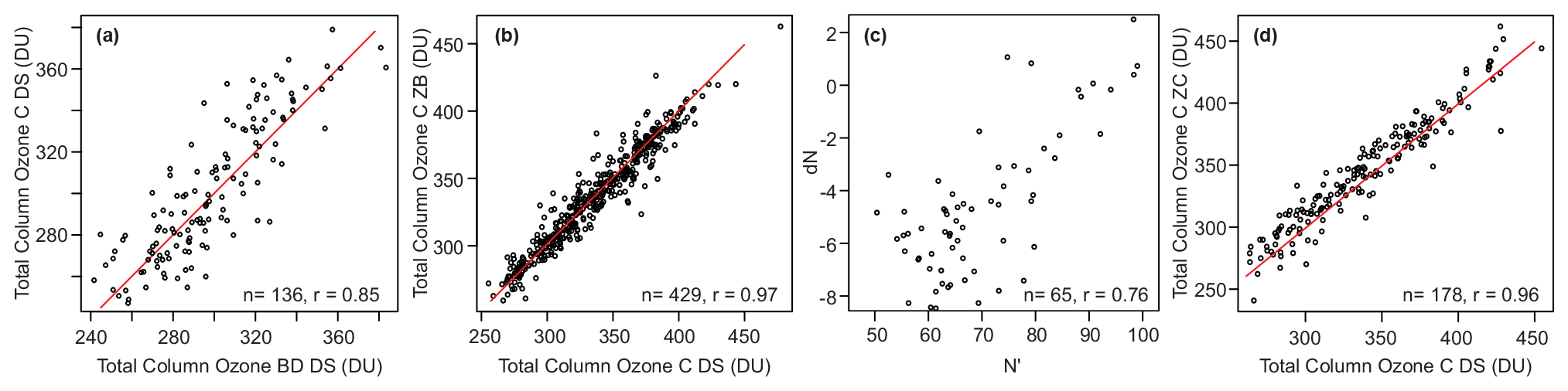
Figure 4 Comparisons of (a) BD and C wavelength pair direct-sun calculations, (b) fitted C ZB data against C DS observations, (c) dN versus N^′ for C ZC observations and (d) reduced C ZC observations versus quasi-simultaneous C DS observations. Here results are shown for the case with Bass–Paur absorption coefficients; plots for the adjusted coefficients are indistinguishable. One-to-one lines are shown in red.

In the next step we compared the C DS data with quasi-simultaneous (<3 h) C ZB data. We identified 429 pairs and applied Eq. (5), stratifying the data into May to October and November to April, respectively. We found an overall good fit (Fig. 4b), with explained variances of 87 and 95 % for the two seasons, respectively (numbers are the same for Bass–Paur or adjusted coefficients). The standard deviations of the residuals were 12 DU for the winter and 9 DU for the summer season.

Next we compared C ZB with C ZC data. We found only 65 quasi-simultaneous observations (Fig. 4c). Separating them into different cloud types was impossible as almost all measurements were for cumulus. We therefore fit only one function, but rather than a linear function as in Vogler et al. (2006) we used a second-order polynomial function. The explained variance of the fit R² was 0.58. The corrections for N that were obtained in this step were then applied to the C ZC data and they were then reduced with the same equation as the C ZB data. As a further test we then selected quasi-simultaneous (<3 h) observations of C DS and C ZC and found 178 pairs (Fig. 4d). The correlation was 0.96 and the standard deviation of the differences amounted to 13 DU, but a mean bias of 5.8 DU (5.7 DU for the case with adjusted coefficients) is apparent. We therefore subtracted 5.8 DU (5.7 DU) from all ZC observations.

In this way all data could be processed. During the process we sometimes discovered inconsistences (e.g. errors in the calculation performed in the 1950s or typos), and some values were marked with question marks on the sheets. While some of the problems (e.g. miscalculations or typos) could be resolved, in other cases such values were flagged in our data set, though we still reduced the ozone amount. We also flagged other suspect values, for example cases where N values were not reduced at all on the sheets. In total, of the 2500 observations digitised, 2253 values were reduced, of which 56 were flagged. By definition of the procedure, DS data are the reference, while ZB data and ZC data are fitted to the DS data in two steps, and thus somewhat lower quality is expected.

Finally, we compared our reduced values to those digitised from the International Ozone Commission files as well as to those stored at WOUDC. This revealed further important information. For instance, January and February 1959 are missing from the International Ozone Commission data but not from our data sheets. The non-reporting could be due to low quality. In fact, many values in January 1959 had question marks on the original sheets, and there is a note that the battery was extremely low; on 4 February battery and spring were replaced, and the rhodium plate was fixed to position “opaque”. In our series, however, only a sequence of values in January 1959 was flagged.

For further comparisons we averaged our values (not considering flagged values) to daily means using New Zealand dates as well as UTC dates and then compared them with the two daily data sets. Both sources (International Ozone Commission and WOUDC) used New Zealand dates, although both are shifted by 1 d after February 1959. After shifting back, we found a generally good agreement. Correlations with the International Ozone Commission and WOUDC data amounted to 0.99 and 0.92, respectively. Discrepancies were checked, which led to the flagging of two additional values, while most checked values were not flagged.

Finally, for the daily data set, we supplemented the half year missing from 1958 with the data from the International Ozone Commission, scaled by 1.041 to account for the change in absorption coefficients. All processed original observations as well as the supplemented daily values are shown in Fig. 5 (here we show the version with Bass–Paur coefficients). No obvious discrepancies are found, although the scatter in the C ZC data is visibly larger than for C DS or C ZB data. In this way the data set is used in the following.

Figure 5 Total column ozone at Downham Market (1950–1951) and Wellington (1951–1959) for different wavelength pairs and observation modes (here for the case of Bass–Paur coefficients).

3.3 Downham Market

In the case of Downham Market, our data are only daily mean reduced total column measurements. All that can be done is to adjust them to account for the change in the absorption cross sections used. At the time of the measurement, the so-called Ny-Choong scale was in use. With the IGY, the Vigroux (1953) scale was adopted, but a few years later it was found to provide inconsistent results and was replaced by an updated Vigroux scale. Finally, the Bass–Paur scale was adopted as the standard (Komhyr et al., 1993). To convert directly from the Ny-Choong to the Bass–Paur scale, we multiplied all values with 1.416, as recommended in Brönnimann et al. (2003b).

Several daily values were illegible, and two were marked with a question mark on the sheet and were correspondingly flagged. The monthly mean values were used to cross-check the numbers. The digitised raw data were then compared with the data from Oxford (Vogler et al., 2007). Using linear regression with Oxford total column ozone as an independent variable, days with exceedingly large residuals (outside ± 3 standard deviations) could be flagged and further checked (e.g. checking for digitising errors or by comparing the value with the days before and after). Only one suspect measurement was found; it was flagged correspondingly.

A very high correlation of 0.91 was found between the series. Although the data only cover 1 year, the difference series showed a clear seasonal cycle, with largest differences approximately around summer solstice. Offsets that include a seasonal cycle are possible due to effects that depend on the solar zenith angle (e.g. due stray light in the instrument), on temperature, on the ozone amount, or on the tropopause height. The data amount is not sufficient to decide between different seasonalities. However, given the very high correlation between the data from Downham Market and Oxford, pointing to a high day-to-day accuracy, we adjusted the Downham Market data by subtracting a seasonal cycle based on fitting the first harmonic to the difference series. Corrections are between 13 DU (winter) and 58 DU (summer).

Repeating the regression approach on this series, we found one additional potential outlier (outside ± 3 standard deviations) that was correspondingly flagged. In this format the series is used further in our paper.

3.4 Data sets used for comparisons

In addition to Oxford total column ozone, which was used for flagging outliers and debiasing the Downham Market record, we used additional historical total column ozone data for several analyses. Specifically, we used total column ozone data from various locations in Europe (Brönnimann et al., 2003b) as well as a historical series from Canberra (1929–1932), which were digitised from daily values in Brönnimann et al. (2003a) and converted to the Bass–Paur scale. While the European data, which were assumed to be of higher quality than some of the other series, are available from the WOUDC, the other series described in Brönnimann et al. (2003a) were only made available via an FTP site, which no longer exists. We are therefore publishing all historical series used in this paper, together with all other series described in Brönnimann et al. (2003a), in an electronic supplement to this paper (Table S1 in the Supplement).

We also used a series from Aspendale near Melbourne, Australia, from the 1950s. Observations with Dobson spectrophotometer #12 began in July 1955. Measurements were taken around noon. Standard observational and calibration procedures were used (Funk and Garham, 1962). The data since the IGY are today found in the WOUDC database. Concerning the earlier data, monthly means are found in various sources (Normand, 1961; Funk and Garham, 1962; and the scans from the International Ozone Commission), but the individual values have so far not been published (the original data sheets are held at the National Archives of Australia). We converted the data to the Bass–Paur scale using a scaling factor of 1.041.

For comparison with later periods (1990s and 2010s), we used total column ozone from the WOUDC database, namely from Lauder, NZ, as well as Melbourne (measurements were performed in the city in the 1990s and at the airport in the 2010s). All locations of the sites are shown in Fig. 1.

Further, we also used zonally averaged total column ozone data sets in order to embed the Wellington series from the 1950s into a long-term and global context. For the 1950s we used the HISTOZ assimilated ozone data set (Brönnimann et al., 2013a, b), which is based on an offline assimilation of historical total column ozone series into an ensemble of chemistry–climate model simulations (note that the monthly Aspendale data from 1955 onward have been assimilated). For the 1990s we used the Zonal Mean Ozone Binary Database of Profiles (BDBP; Bodeker et al., 2013), and for the 2010s we used the MOD7 release of the Solar Backscatter Ultraviolet Radiometer data set (SBUV Version 8.6) merged total and profile ozone data set (Frith et al., 2014).

Comparisons were also performed with radiosonde and other upper-level data. We used radiosonde data from IGRA2 (Durre et al., 2016, 2018) originating back to TD54 (see Stickler et al., 2010). We used data from Auckland (1949–1957) for comparison with the Wellington ozone data (at 490 km distance) and from Invercargill Airport (1950–2020) for comparison with Lauder ozone data (at 180 km distance) for the period 1987–2010. Radiosonde data from Norfolk Island (1943–2020) were also used for analysing spatial patterns. For the Downham Market data, no nearby radiosonde station was available. We compared the total column ozone data with geopotential height and temperature at all levels from the surface to the lower stratosphere. All three stations were used to check the flow field for individual days. The locations of the stations are also shown in Fig. 1.

It is also interesting to compare total column ozone from our historical observation with that in reanalyses. In fact, total ozone can be used to assess the quality of reanalyses (Brönnimann and Compo, 2012; Hersbach et al., 2017). Here we compare both historical total column ozone data series with the three reanalysis data sets ERA-PreSAT, 20CRv3 (Slivinski et al., 2019a, b), and CERA-20C (Laloyaux et al., 2018). For the processing, as in Brönnimann and Compo (2012) and Hersbach et al. (2017), all data were deseasonalised by subtracting the first two harmonics of the seasonal cycle, and then Pearson correlations were calculated. For the case of Downham Market, which only covers 1 year, we fitted only the first harmonic function.

4 Results

4.1 Wellington

Results of the correlation between Auckland radiosonde data and total column ozone in Wellington are given in Table 2. For comparability purposes, we performed the same analysis for a more recent period (1987–2010), with Invercargill radiosonde data and total column ozone measurements in Lauder. From all series, the first two harmonics of the seasonal cycle were subtracted; then the anomalies were correlated. As expected for a mid-latitude site, we find negative correlations with geopotential height at all levels, but strongest near the tropopause and decreasing towards the surface and towards the stratosphere. For temperatures, correlations change sign at the tropopause; i.e. high total column ozone is related to a low tropopause altitude, a cold upper troposphere, and a warm lower stratosphere.

Table 2 Correlation coefficients (after deseasonalising) between total column ozone at Wellington and radiosonde geopotential height (GPH) and temperature (T) at Auckland (1951–1957) as well as total column ozone at Lauder and radiosonde data at Invercargill (1987–2010); see Fig. 1 for locations.

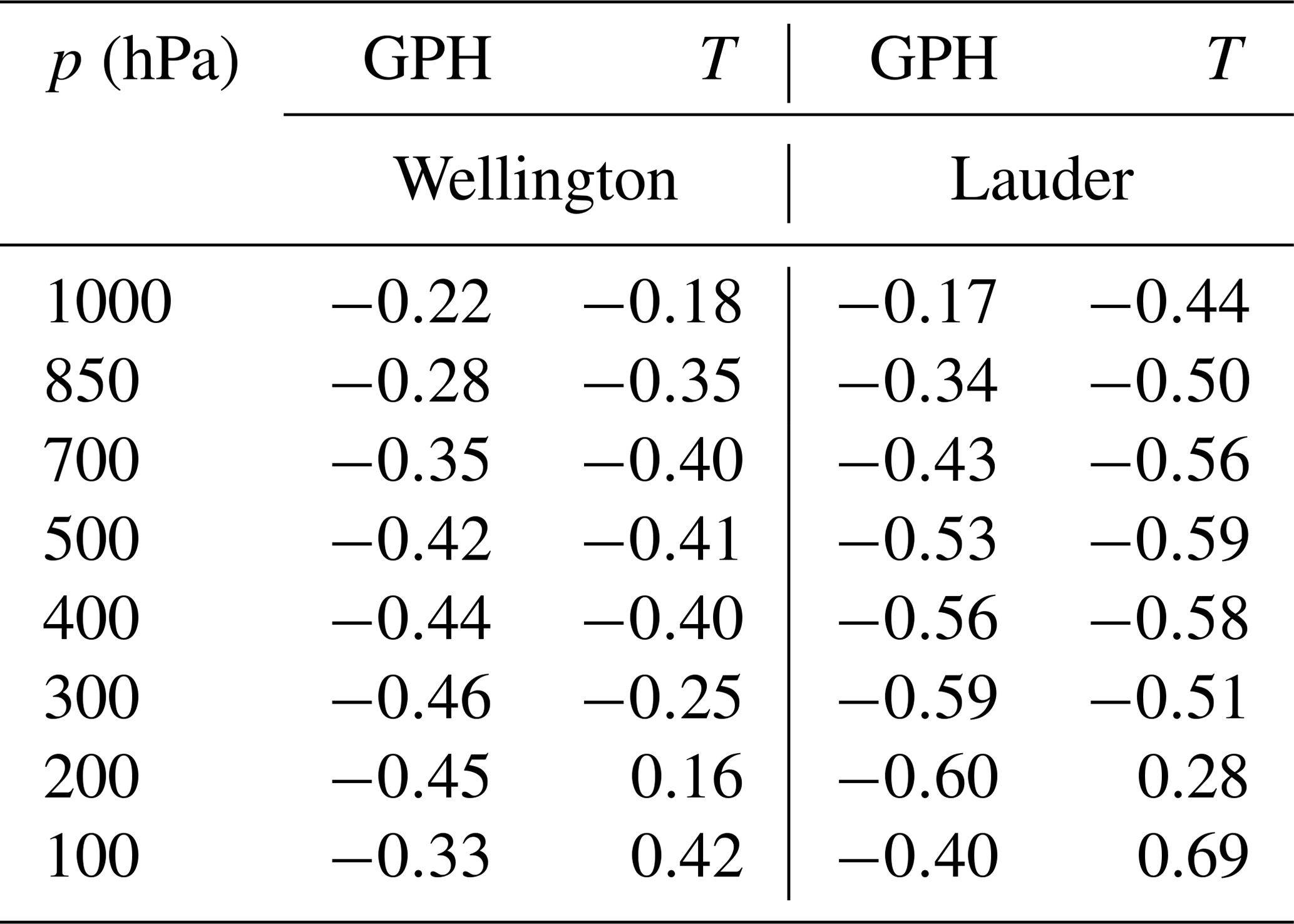
Correlations are lower for the historical period than for the recent period. Differences could be explained not only by the shorter spatial distance between Lauder and Invercargill (180 km) than between Wellington and Auckland (490 km) and also the shorter temporal distance (in the historical period radiosondes were launched once per day, first at 11:00 UTC and later at 00:00 UTC, whereas in the second period we have twice-daily soundings, of which we chose the closer) but also by the lower quality of both data sources (ozone measurements and radiosonde). Nevertheless, with correlations approaching −0.5 at the tropopause level, results show that day-to-day variability in total column ozone is likely to be well captured.

Next we compared Wellington ozone with ozone from reanalysis data sets (Table 3). Absolute values of the reprocessed Wellington observations are 5.5 % (adjusted coefficients) or 8 % (Bass–Paur) higher than those from the reanalyses. This is not due to outliers or specific periods but seems to be a feature of the bulk data. Correlations are lower than for Downham Market, as expected since in the area of New Zealand the reanalyses are not well constrained. Nevertheless, we find correlations of around 0.6 to 0.8 for absolute values and of 0.45 for anomalies. The lowest correlations on the anomalies are again found for CERA-20C. There is no clear difference between the observation modes, except that the “infilled” daily data from the International Ozone Commission are slightly worse (pointing to the value of working with original material).

Table 3 Correlation coefficients (before and after deseasonalising) between total column ozone at Wellington and in other data sets (1951–1959) for different wavelengths and observation modes (the table relates to the case of Bass–Paur coefficient; results are almost indistinguishable for the adjusted coefficients).

We also analysed some specific days. Figure 6 shows a day with particularly high total column ozone in the series of Wellington. High ozone values at mid-latitudes are mostly due to upper-level troughs. The reanalyses ERA-PreSAT and 20CRv3 both reproduce higher ozone values related to an upper trough (100 hPa geopotential height is also indicated) but do not reproduce the absolute value. 20CRv3 shows stronger gradients in both fields.

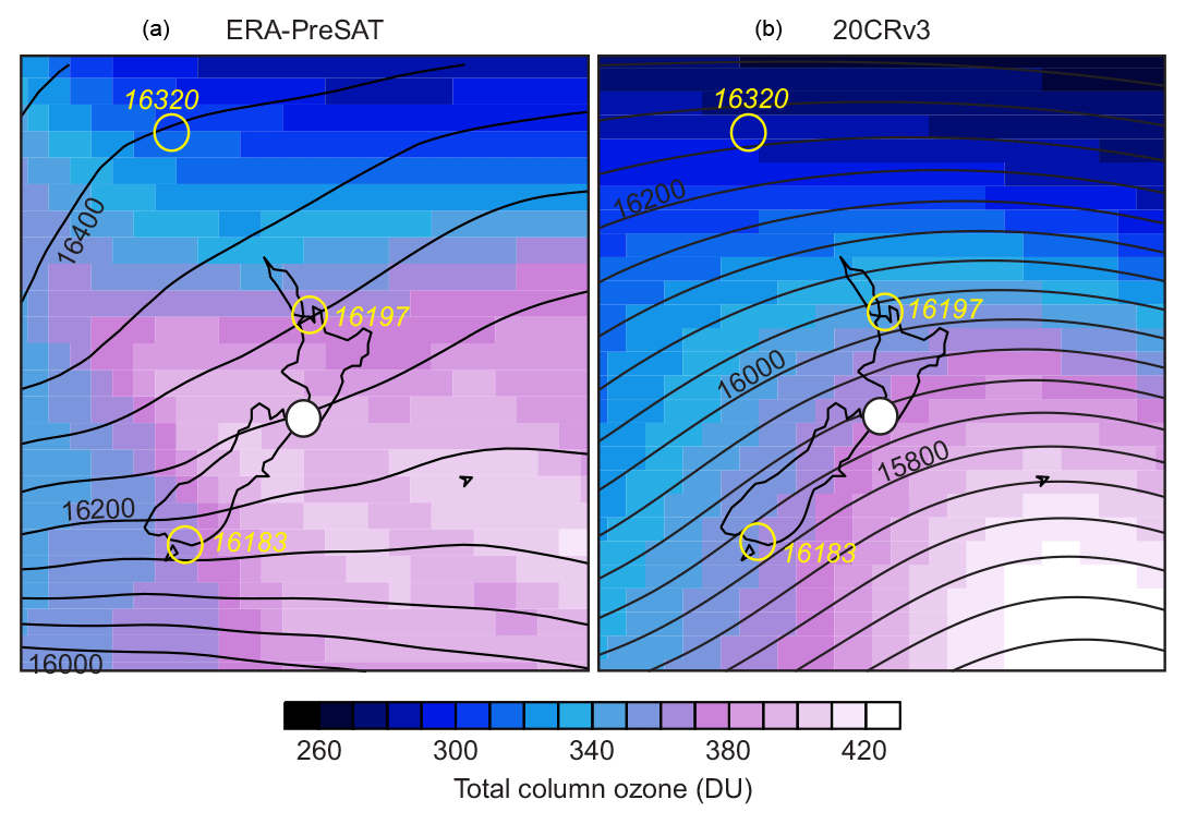
Figure 6 Total column ozone and 100 hPa geopotential height on 25 September 1952 in ERA-PreSAT (a) and 20CRv3 (b). The filled circle indicates the measured total column ozone value at Wellington (434.6 DU, adjusted coefficients); open circles indicate geopotential height from radiosonde (taken 12 h later).

4.2 The long-term view

Finally, we also put the reanalysed series from Wellington in a long-term context (Fig. 7). We compared the decadally averaged seasonal cycle for the 1950s (both for the Bass–Paur coefficients and the adjusted coefficients) with that from Lauder from the 1990s (corresponding to the peak of ozone depletion) and the 2010s. At least 10 days were required to form a monthly average from which decadal averages were then taken. Also shown in the same figure are data from Aspendale/Melbourne for the three periods, and to the plot of the first period we also added the Canberra (1929–1932) series. Note that Canberra and Melbourne are further north than Wellington, while Lauder is further south. To make ozone at the different latitudes comparable, we added offsets that were calculated from MOD7 zonal averaged data (differences between the corresponding latitudes).

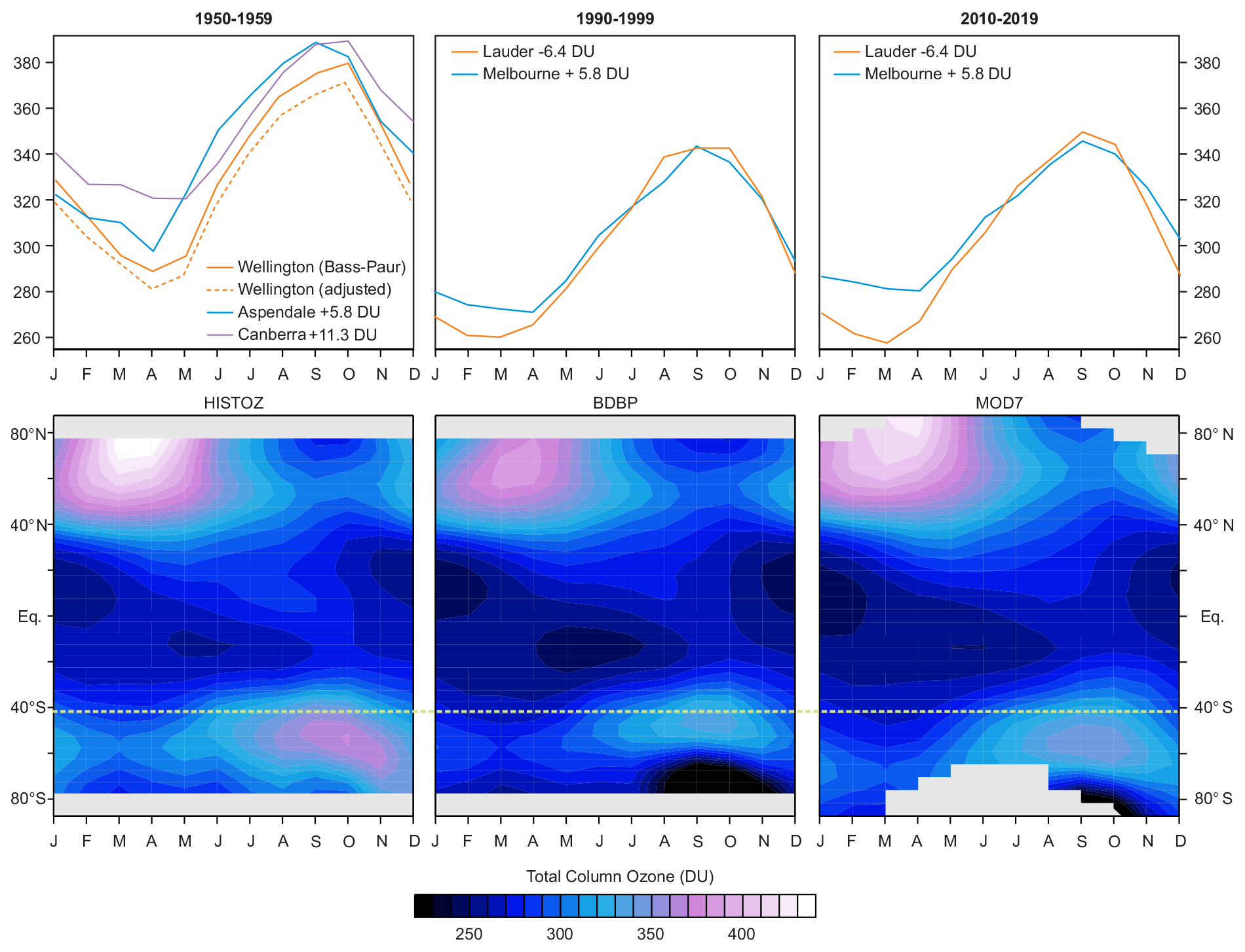
Figure 7 Top: decadally averaged annual cycle from total column ozone measurements in New Zealand and Australia in the 1950s, 1990s, and 2010s. Note that the series are adjusted according to the annual mean offset between the corresponding latitudes and that of Wellington in MOD7. Bottom: zonally averaged total column ozone as a function of calendar month and latitude in the data sets HISTOZ (1950s), BDBP (1990s), and MOD7 SBUV merge (2010s). The bottom left and middle panels are from Brönnimann (2015). Lauder and MOD7 data end in 2018. The dashed line indicates the latitude of Wellington. Grey: no data.

For the same three periods we also show zonal average total column ozone as a function of latitude and calendar month in the assimilated total ozone data set HISTOZ (Brönnimann et al., 2013a, b; note that this data set does not assimilate the Wellington data) for the 1950s, together with corresponding data from BDBP (Bodeker et al., 2013) for the 1990s and from the MOD7 SBUV merged data set for the 2010s. Note that the latitude–calendar month plots are based on three different data sets. However, HISTOZ is by construction consistent with BDBP, and the difference between MOD7 and BDBP is small. From 55^∘ S to 60^∘ N the standard deviation of the differences in zonally averaged monthly total column ozone between the data sets is below 10 DU; the mean difference at 42.5^∘ S amounts to 5.5 DU.

For the 1950s, the shape of the curves agrees well, but there are considerable differences in the levels, reflecting the uncertainty in absolute values. The Wellington curve with adjusted coefficients is the lowest; the Canberra series is (on average) the highest. Comparing the figures for the 1950s and the 1990s, we find a large decrease between the two time periods. This decrease is much stronger than the uncertainty between the data sets. Both in the station data as well as in the global data set the change from the pre-ozone depletion climatology to the maximum decade of ozone depletion, the 1990s, is thus clearly visible. Ozone depletion is visible not just over Antarctica in spring but also year round at southern mid-latitudes and in the subtropics. From the 1990s to the 2010s, a slight increase is seen at most latitudes in MOD7, but hardly near 40^∘ S. Likewise, only a faint increase is seen in the Lauder observations.

4.3 Downham Market

Table 4 lists the correlations between the re-evaluated Downham Market data (without the flagged values) and other total column ozone series before and after deseasonalising. Note that for the reanalyses 20CRv3 and CERA-20C we used the ensemble mean. Correlations are generally high. Even with the series of Arosa (at almost 1000 km distance), a correlation of 0.78 was found (not shown). For the nearby Oxford series as well as for ERA-PreSAT, correlations exceed 0.90 on the absolute values and 0.75 on the anomalies. The corresponding scatter plot (Fig. 8) for these two cases shows a linear relation with no apparent deviations for high or low values. The 20CRv3 reanalysis, which in contrast to ERA-PreSAT does not assimilate upper-level variables, also shows very high correlations. Slightly lower correlations are found for CERA-20C.

Table 4 Pearson correlation coefficients of the re-evaluated total column ozone series from Downham Market with other column ozone series. Anomalies refer to the values after subtracting the first harmonic function in terms of day of year.

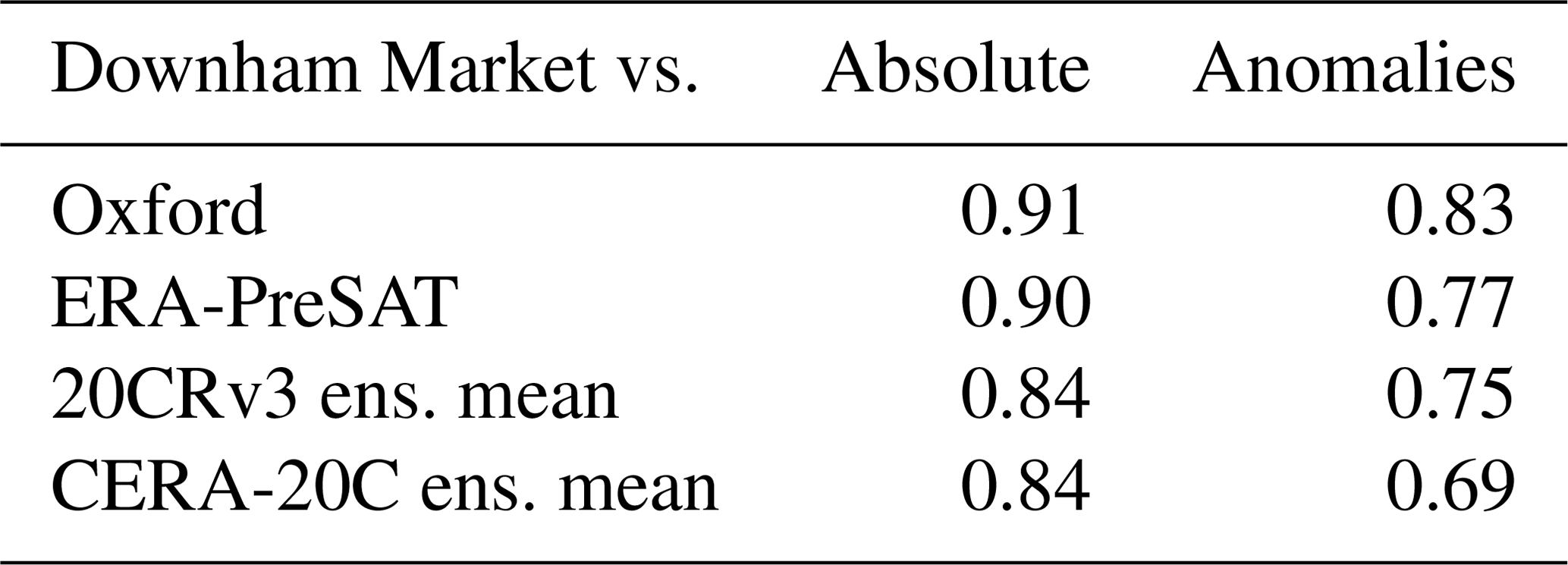
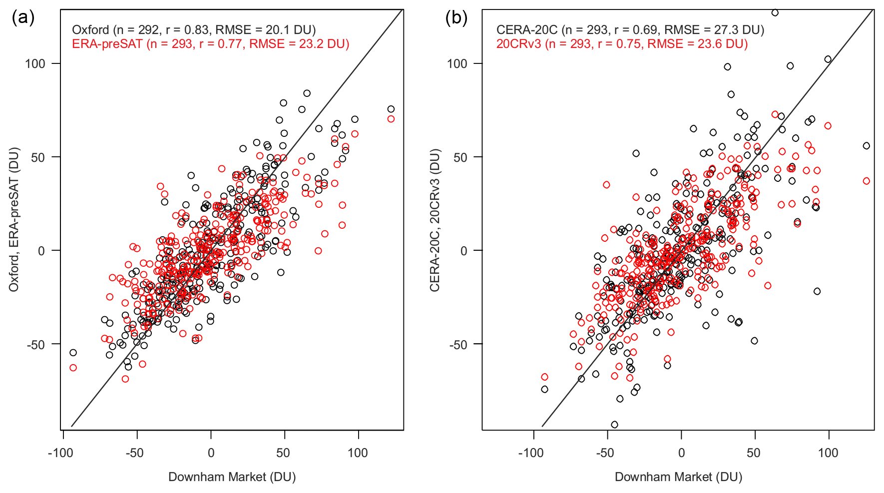
Figure 8 Scatter plot of deseasonalised total column ozone data at Downham Market against (a) measurements performed in Oxford as well as total column ozone data from the closest grid cell in ERA-PreSAT and (b) total column ozone data from the closest grid cell in 20CRv3 and CERA-20C (ensemble mean). The one-to-one line is shown in black. The numbers in brackets indicate the number of data points, correlations, and root mean squared errors in DU.

We also analysed ozone fields for individual days. For this we supplemented the Downham Market ozone observations with other observations from Europe, as given in Brönnimann et al. (2003b). Five days were selected with good data coverage and pronounced positive or negative anomalies of observed total column ozone over Downham Market. For these days, observed ozone is plotted together with ozone from ERA-PreSAT (Fig. 9). We find a good agreement between Downham Market and neighbouring stations as well as with ERA-PreSAT total column ozone fields in all cases (over the entire record, the standard deviation of differences is 25.9 DU). In fact, most of the stations show a good agreement (in the range of 30 DU), in this sense confirming the value of historical total column ozone data.

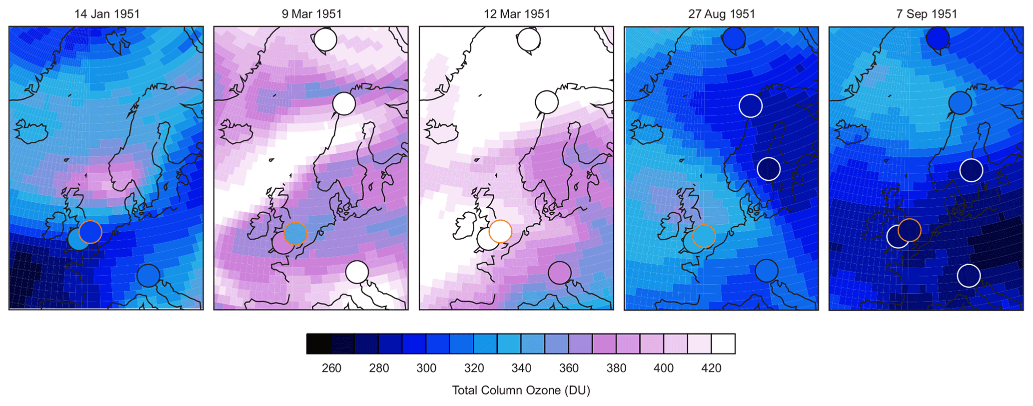
Figure 9 Total column ozone in ERA-PreSAT as well as in observations from various stations on five days in the year 1951 (Downham Market is marked with an orange outline of a circle).

5 Discussion

The re-evaluated total column ozone series from Wellington is internally consistent, although its absolute level remains difficult to assess in the absence of calibration information. From the comparisons in Fig. 3 and assuming that in any comparison both series contribute roughly equally to the error of the difference, a standard deviation of 13 DU in the difference between two series is equivalent to a random error (standard deviation) of 9 DU in each of the two series. We can therefore assume that in the reprocessed Wellington series the random error (in terms of a standard deviation) is better than 10 DU. The systematic error is of approximately the same magnitude. The choice of the absorption coefficients leads to a difference of 8.8 DU; however, other uncertainties add to this. Comparisons with not only reanalysis data but also HISTOZ suggest that the Wellington data are too high, but comparisons with Aspendale and Canberra data (albeit of even lower quality) suggest that the data are too low. Too-high values could be due to calibration errors, or due to a too-small aerosol correction. However, high values are also possible for dynamical reasons such as a negative phase of the Southern Annular Mode (SAM). In fact, pressure reconstructions indicate a sequence of years with negative SAM in the 1950s (Fogt et al., 2009, 2016). In any case, we recommend using the Wellington series with the adjusted coefficients, which best uses all information in the possession of the authors, although important pieces of information are lacking.

The Downham Market data are surprisingly precise, with a much higher correlation with independent data than the data from Wellington. Also the absolute level is arguably better determined as this series is statistically adjusted, while the Wellington data are completely independent from any other series. However, despite the good statistical performance, the Downham Market data are of different quality merely based on the fact that we do not have raw data.

Both the Downham Market, UK, and Wellington, NZ, data depict day-to-day variability well, which is closely related to the flow near the tropopause (Steinbrecht et al., 1998). This is evidenced by the high correlation with radiosonde data in the case of Wellington and points to good quality of the ozone data. Note that lower correlations between total ozone and upper-level variables are expected at the southern mid-latitudes than at northern mid-latitudes (see Brönnimann and Compo, 2012). However, as we have no calibration information and no intercomparison data, the series may not have trend quality.

For Downham Market, a large correction was necessary, but correlation with Oxford ozone observations likewise suggests high quality with respect to short-term changes, which is surprising given the almost illegible data sheets. However, both the Oxford series and the Downham Market series might have been affected by tropospheric aerosols. This was the reason why Dobson did not consider the Oxford series as very valuable for science, and the same might also be the case for Downham Market.

Once the reliability of day-to-day variations in the ozone data is established, they can be used to assess historical reanalysis products. In Brönnimann and Compo (2012), anomaly correlations between observed and 20CRv2 ozone in Christchurch (in the 1920s) were found to be around 0.5 (a similar value to that for Wellington); for Europe anomaly correlations exceeding 0.6 were found. Hersbach et al. (2017) found anomaly correlations of 0.6 to 0.8 for total column ozone in ERA-PreSAT, which is similar to what we find for Downham Market. We find even higher correlations in our case, which might be due to better data but more likely also reflects improvements in the reanalysis products.

Note that the quality of the Wellington data has not been tested for use in trend studies, and we recommend not using the data for trend analysis given the reported problems with the instrument. Together with other data sources, the series nevertheless provides a glimpse at ozone variability in the pre-ozone depletion era, which can be compared to later periods. All data sources together illustrate a decrease in total column ozone from the 1950s to the 1990s, approximately the time of minimum ozone (Solomon, 1999; Staehelin et al., 2001). An increase is found in some data sets and stations since then and interpreted as a sign of ozone recovery (Solomon et al., 2016). In the case of the southern mid-latitude, an increase from the 1990s to the 2010s is hardly detectable. Historical data such as those from Wellington are valuable as they depict ozone at southern mid-latitudes prior to the onset of ozone depletion. Taken together, the data indicate that recovery is still far from complete. Values have not nearly returned to the 1950s state.

6 Conclusions

Historical total column ozone data are relevant not just for analyses of long-term changes in the ozone layer but also as a diagnostic of day-to-day atmospheric dynamics near the tropopause. In this paper we present historical series from Wellington, New Zealand, from 1951 to 1959 and Downham Market, UK, from November 1950 to October 1951. The data are re-evaluated and analysed with respect to their quality. The former series will be made available via the World Ozone and Ultraviolet Data Centre. Both series are published in the Supplement, together with other historical total column ozone series used in this paper and described in Brönnimann et al. (2003a).

The analyses reveal a good depiction of day-to-day variability, a fact which can be used to assess the quality of reanalysis products, since the data cover a region and time period with only few upper-air data. We show comparisons with the three reanalyses ERA-PreSAT (which assimilates upper-air data), 20CRv3, and CERA-20C, all of which show high correlations, particularly over Europe but also over New Zealand. Eventually, historical total column ozone data could also be assimilated into historical reanalysis products.

The Wellington data were combined with other data sources to assess long-term ozone changes over New Zealand. The 1950s in this context represent the era prior to the onset of ozone depletion. Together, the data suggest that the recovery of the ozone is underway but is still far from the state it had in the 1950s. It should be noted, however, that the historical Wellington data arguably do not have trend quality.