Assessment of regional aerosol radiative effects under the SWAAMI campaign – Part 2: Clear-sky direct shortwave radiative forcing using multi-year assimilated data over the Indian subcontinent

Clear-sky, direct shortwave aerosol radiative forcing (ARF) has been estimated over the Indian region, for the first time employing multi-year (2009–2013) gridded, assimilated aerosol products, as an important part of the South West Asian Aerosol Monsoon Interactions (SWAAMI) which is a joint Indo-UK research field campaign focused at understanding the variabilities in atmospheric aerosols and their interactions with the Indian summer monsoon. The aerosol datasets have been constructed following statistical assimilation of concurrent data from a dense network of ground-based observatories and multi-satellite products, as described in Part 1 of this two-part paper. The ARF, thus estimated, is assessed for its superiority or otherwise over other ARF estimates based on satellite-retrieved aerosol products, over the Indian region, by comparing the radiative fluxes (upward) at the top of the atmosphere (TOA) estimated using assimilated and satellite products with spatiotemporally matched radiative flux values provided by CERES (Clouds and Earth's Radiant Energy System) single-scan footprint (SSF) product. This clearly demonstrated improved accuracy of the forcing estimates using the assimilated vis-à-vis satellite-based aerosol datasets at regional, subregional and seasonal scales. The regional distribution of diurnally averaged ARF estimates has revealed (a) significant differences from similar estimates made using currently available satellite data, not only in terms of magnitude but also the sign of TOA forcing; (b) the largest magnitudes of surface cooling and atmospheric warming over the Indo-Gangetic Plain (IGP) and arid regions from north-western India; and (c) negative TOA forcing over most parts of the Indian region, except for three subregions – the IGP, north-western India and eastern parts of peninsular India where the TOA forcing changes to positive during pre-monsoon season. Aerosol-induced atmospheric warming rates, estimated using the assimilated data, demonstrate substantial spatial heterogeneities (∼0.2 to 2.0 K d⁻¹) over the study domain with the IGP demonstrating relatively stronger atmospheric heating rates (∼0.6 to 2.0 K d⁻¹). There exists a strong seasonality as well, with atmospheric warming being highest during pre-monsoon and lowest during winter seasons. It is to be noted that the present ARF estimates demonstrate substantially smaller uncertainties than their satellite counterparts, which is a natural consequence of reduced uncertainties in assimilated vis-à-vis satellite aerosol properties. The results demonstrate the potential application of the assimilated datasets and ARF estimates for improving accuracies of climate impact assessments at regional and subregional scales.

1 Introduction

The uncertainties in aerosol radiative forcing (ARF) pose primary challenges in the assessment of climatic implications of atmospheric aerosols at global, regional and even subregional scales (Schwartz, 2004; Boucher et al., 2013). In order to improve the estimates of aerosol climate sensitivity, an at least 3-fold reduction in the uncertainties in aerosol radiative forcing is necessary (Schwartz, 2004). Despite efforts towards this, significant uncertainties still persist in the estimates of even direct aerosol radiative forcing (DARF) (Penner et al., 1994; Boucher and Anderson, 1995; Ramanathan and Carmichael, 2008), aside from the indirect forcing. This calls for improvement in the accuracy of primary aerosol inputs to DARF estimation at subregional and regional scales.

There have been several estimates of global ARF by employing general circulation models (GCMs) or chemistry transport models (CTMs) making use of aerosol emission inventories (Jacobson, 2001; Takemura et al., 2002; Myhre et al., 2007, 2009; Kim et al., 2008). These studies have highlighted the regional and temporal heterogeneity in aerosol forcing, but the actual forcing values reported have significant uncertainties emanating mainly from those in the input inventories, meteorology and assumptions made in aerosol–chemistry processing. Schulz et al. (2006) have shown that the model-based (GCM or CTM) estimates of radiative forcing differ significantly amongst themselves, even in terms of sign of radiative forcing, despite using identical emission inventories. Recognizing this issue, Chung et al. (2005, 2010) have produced global and regional maps of aerosol forcing employing observationally constrained aerosol datasets, which were constructed by integrating satellite and ground-based observations of aerosol optical depth (AOD) with those derived from the global Goddard Chemistry Aerosol Radiation and Transport (GOCART) model. They provided somewhat more realistic estimates of aerosol forcing compared to those incorporating model-derived aerosol parameters because of the improvements in the input datasets arising from their assimilation efforts. Nevertheless, due to limited number of regional ground stations involved in the assimilation process by Chung et al. (2005) (for example, only two stations over the Indian region), the assimilated AODs over large parts of the globe remained largely represented by satellite-retrieved and model-derived AODs, which suffer from significant uncertainties and biases emanating from a variety of sources (cloud contamination, spatial heterogeneities in surface albedo, sparse temporal sampling, various assumption made during the retrieval procedure and sensor degradation, etc.) (Zhang and Reid, 2006; Jethva et al., 2014). As a result, large uncertainties still prevailed at regional and subregional scales.

Location-specific estimates are more accurate as these employ highly accurate ground-based measurements of aerosol properties (spectral AOD, aerosol absorption, altitude profiles, etc.) and generate aerosol models constrained with measurements and use them in a radiative transfer scheme (Babu and Moorthy, 2002; Suresh Babu et al., 2007; Satheesh et al., 2006; Pathak et al., 2010; Sinha et al., 2013). Due to smaller uncertainties in the direct measurements, these aerosol forcing estimates tend to have lesser uncertainties vis-à-vis forcing estimates from satellite-retrieved and model-derived aerosol parameters. However, due to limited spatial representativeness of each ground station and the limited density of ground networks, these ARF estimates are highly location specific. They lack the much-needed regional representativeness for climate assessment, unless they involve a large number of ground locations, from a highly dense network, which has associated practical difficulties. Recognizing these scenarios, especially over the Indian region which has large spatiotemporal variations in aerosol properties, a careful assimilation of moderately dense network data with satellite data to generate a gridded dataset which is more or less continuous in space and time has been envisioned as one of the key objectives by the South West Asian Aerosol Monsoon Interactions (SWAAMI; https://gtr.ukri.org/projects?ref=NE/L013886/1, last access: 9 May 2020), a coordinated field campaign jointly undertaken by the scientists from India and the United Kingdom.

In Part 1 of this two-part paper, we have presented the gridded, assimilated datasets of AOD and single scattering albedo (SSA) over India, which provide spatiotemporally continuous data, generated for the first time by harmonizing long-term (2009–2013) measurements from a dense network of ground-based aerosol observatories and multi-satellite datasets following statistical assimilation techniques (Pathak et al., 2019). The resulting improvement in accuracies of the gridded products (over the parent data) in reproducing the spatiotemporal characteristics of aerosol properties at subregional scales over the Indian domain was also demonstrated. In Part 2 of the paper, we have estimated the direct shortwave aerosol ARF over the Indian region using the above gridded data and examined its features. A comparison of these estimates is done with similar estimates made using the parent satellite data to demonstrate the effectiveness of the assimilated data in better quantifying ARF over the Indian region with its characteristic spatiotemporal features. Further, we have compared the top-of-the-atmosphere (TOA) flux estimated using the assimilated data with the instantaneous flux values measured by the Clouds and Earth's Radiant Energy System (CERES) instrument, and the seasonal contrast in ARF is then presented for various geographically homogeneous subregions. The primary findings of the present work are then summarized.

2 Database

Accuracy of estimation of direct aerosol radiative effect depends strongly on the accuracies of three key optical properties of aerosols, namely AOD, SSA and single-scatter phase function, and the availability of these continuously in space and time over the domain of interest. Accordingly, in this work, we have used the gridded data over the Indian domain for AOD and SSA at $\mathrm{1}{}^{\circ }\times \mathrm{1}{}^{\circ }$ resolution. These datasets are generated by assimilating long-term data from ground-based network observatories and space-borne sensors following statistical assimilation techniques (3D-Var and weighted interpolation methods) as described in Pathak et al. (2019) (Part 1) and are available at http://dccc.iisc.ac.in/aerosoldata/ (last access: 9 May 2020). These assimilated AOD and SSA are henceforth, respectively, denoted as AS AOD and AS SSA. However, such a comprehensive dataset for aerosol phase function is not available over the study domain, and as such we relied on the Optical Properties of Aerosols and Clouds (OPAC) model (Hess et al., 1998), which provides optical properties for variety aerosol species and their mixtures (under externally mixed assumption). As our study domain is mainly comprised of land areas, an average value of aerosol phase function (at 550 nm) corresponding to all continental aerosol mixtures in OPAC is considered, and its Legendre polynomial coefficients (eight streams) are employed for determining the Legendre moments of the phase function.

In addition to assimilated aerosol products, we have also employed satellite-retrieved AOD and SSA (denoted as SR AOD and SR SSA, respectively) for ARF estimation. The satellite-retrieved AODs employed here are constructed by combining by monthly averaged AOD products ($\mathrm{1}{}^{\circ }\times \mathrm{1}{}^{\circ }$ resolution) from (L3, Collection 6; https://modis.gsfc.nasa.gov/data/, last access: 9 May 2020) MODerate Imaging Spectroradiometer (MODIS) aboard the Aqua and Terra satellites as well as from Multiangle Imaging SpectroRadiometer (MISR) aboard the Terra satellite (L3; https://misr.jpl.nasa.gov/, last access: 9 May 2020) (Diner et al., 1998), as detailed in Part 1 of the two-part paper (Pathak et al., 2019). The satellite-retrieved SSAs are provided by monthly mean SSA (at 500 nm) datasets constructed from upwelling radiance measurements (in the range of 270–500 nm) performed by the Ozone Monitoring Instrument (OMI) aboard the Aura satellite (Torres et al., 2007; Levelt et al., 2006).

The spatial distributions of the gridded aerosol properties (assimilated as well as satellite retrieved; AODs and SSA) are shown in Fig. 1 for two typical months; January – typical winter, when the majority of aerosols are trapped near the surface due to the shallow atmospheric boundary layer; and May – typical summer/pre-monsoon when the strong thermal convection ensures a thorough vertical mixing within the deep atmospheric boundary layer (ABL) (Kompalli et al., 2014). These two months also signify periods when the local emissions dominate in the aerosol loading (winter) and when advected aerosols (dust and sea salt) also contribute significantly to the aerosol loading (summer/pre-monsoon) (Moorthy et al., 2005; Krishna Moorthy et al., 2007; Jethva et al., 2005; Niranjan et al., 2007). Subregional differences in the spatial distribution of these parameters between the assimilated and satellite-retrieved products are noticeable in Fig. 1, the most conspicuous being in SSA where the assimilated data show stronger absorption than the satellite-retrieved data over many parts of the domain.

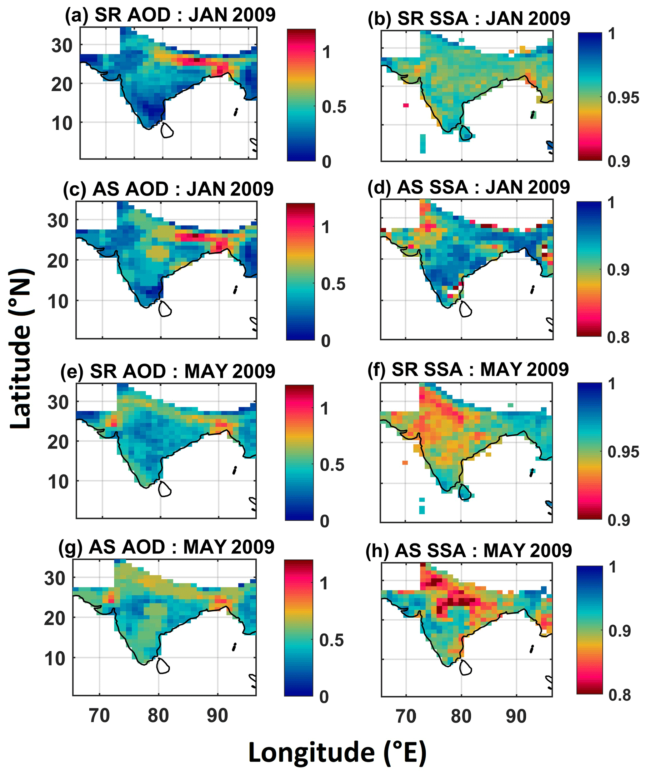
Figure 1 Spatial variation of (a) SR AOD for January 2009, (b) SR SSA for January 2009, (c) AS AOD for January 2009, (d) AS SSA for January 2009, (e) SR AOD for May 2009, (f) SR SSA for May 2009, (g) AS AOD for May 2009 and (h) AS SSA for May 2009.

3 ARF estimation

For estimating aerosol radiative forcing, we have used the Santa Barbara DISORT Atmospheric Radiative Transfer (SBDART) radiative heat transfer model, which uses the DIScrete Ordinate Radiative Transfer (DISORT) algorithm to solve the radiative heat transfer equation with plane-parallel assumption, in the atmosphere with vertical inhomogeneities (Ricchiazzi et al., 1998). The above-described columnar AOD and SSA (Sect. 2) data are used as inputs. Here, the aerosols are considered to be exponentially distributed in vertical direction with the typical scale height of 1.45 km (Ricchiazzi et al., 1998). The surface reflectance data needed have been taken from MODIS, while vertical distribution of atmospheric gases, except columnar ozone and water vapour, is specified using the tropical environment model provided by SBDART. For columnar ozone and water vapour, datasets for the corresponding period provided, respectively, by OMI and MODIS are used (Ziemke et al., 2006; Gao and Kaufman, 2003). The upward and downward shortwave fluxes at TOA and the surface, (in the wavelength range of 0.2 to 4 µm) are computed using SBDART for each hour from 06:00 (approximate local sunrise time in Indian Standard Time; IST) to 18:00 (approximate local sunset time in IST) for each grid point. The net radiative fluxes are then estimated (considering upward negative and downward positive) for “with aerosol” and “without aerosol” conditions and then ARF is estimated as the difference between the net fluxes for the two conditions as has been described in Eqs. (1)–(2).

$$\begin{array}{}\text{(1)}& {\displaystyle }\begin{array}{rl}\mathrm{AS}{\mathrm{ARF}}_{\mathrm{TOA}}^{\ast }& ={\left(F{\downarrow }_{\mathrm{TOA}}-F{\uparrow }_{\mathrm{TOA}}\right)}_{\mathrm{with}\mathrm{aerosol}}\\ & -{\left(F{\downarrow }_{\mathrm{TOA}}-F{\uparrow }_{\mathrm{TOA}}\right)}_{\mathrm{no}\mathrm{aerosol}}\end{array}\text{(2)}& {\displaystyle }\begin{array}{rl}\mathrm{AS}{\mathrm{ARF}}_{\mathrm{srf}}^{\ast }& ={\left(F{\downarrow }_{\mathrm{srf}}-F{\uparrow }_{\mathrm{srf}}\right)}_{\mathrm{with}\mathrm{aerosol}}\\ & -{\left(F{\downarrow }_{\mathrm{srf}}-F{\uparrow }_{\mathrm{srf}}\right)}_{\mathrm{no}\mathrm{aerosol}}\end{array}\end{array}$$

Here, AS ARF^∗ denotes aerosol radiative forcing estimated using assimilated aerosol properties, while the subscripts TOA and srf denote the top of atmosphere and ground surface, respectively, for a given grid point and solid angle. The upward and downward fluxes over the shortwave spectrum are, respectively, denoted by F↑ and F↓. The corresponding atmospheric forcing (denoted by AS ARF${}_{\mathrm{atm}}^{\ast }$) due to aerosols absorption is then estimated as shown in the following (Eq. 3).

$$\begin{array}{}\text{(3)}& \mathrm{AS}{\mathrm{ARF}}_{\mathrm{atm}}^{\ast }=\mathrm{AS}{\mathrm{ARF}}_{\mathrm{TOA}}^{\ast }-\mathrm{AS}{\mathrm{ARF}}_{\mathrm{srf}}^{\ast }\end{array}$$

The ARF values estimated in Eqs. (1)–(3), which are specific to a solar-zenith angle (or time of the day) for a given location, are further averaged (over the period of 12 h) and then halved in order to estimate the diurnally averaged shortwave ARF for the given grid point. These diurnally averaged ARF at the TOA, surface and in the atmosphere are henceforth referred to as AS ARF_TOA, AS ARF_srf and AS ARF_atm, respectively (without an asterisk).

With a view towards assessing the improvements (or otherwise) of the current estimates over such estimates made using conventional (satellite-retrieved or ground-measured) datasets, we have also estimated direct ARF by using only the satellite-retrieved aerosol products (AOD and SSA) in SBDART for the same period, over the same domain. All other input parameters are kept the same as for AS dataset. The diurnally averaged ARF estimates corresponding to satellite products, at TOA, surface and within the atmosphere are henceforth referred to as SR ARF_TOA, SR ARF_srf and SR ARF_atm, respectively.

It is to be noted that we have first estimated the upward and downward shortwave radiative fluxes at TOA and surface for each hour from 06:00 (approximate local sunrise time in IST) to 18:00 (approximate local sunset time in IST) by incorporating assimilated and satellite-based aerosol properties into the radiative transfer model for each grid point. The net radiative fluxes are then estimated (considering upward fluxes negative and downward fluxes positive) for “with aerosol” and “without aerosol” conditions, and then radiative forcing (RF) is estimated as the difference between the net fluxes for the two conditions as has been described in Eqs. (1)–(3) from the paper. These ARF values, which are specific to a solar-zenith angle (or time of the day) for a given location, are further averaged (over the period of 12 h) and then halved in order to estimate the diurnally averaged shortwave ARF for the given grid point.

Further, from each of the forcing estimates made using the two different datasets, we also estimated the difference between the two (referred to as dARF) as

$$\begin{array}{}\text{(4)}& {\displaystyle }{\mathrm{dARF}}_{\mathrm{TOA}}=\mathrm{AS}{\mathrm{ARF}}_{\mathrm{TOA}}-\mathrm{SR}{\mathrm{ARF}}_{\mathrm{TOA}}\text{(5)}& {\displaystyle }{\mathrm{dARF}}_{\mathrm{srf}}=\mathrm{AS}{\mathrm{ARF}}_{\mathrm{srf}}-\mathrm{SR}{\mathrm{ARF}}_{\mathrm{srf}}\text{(6)}& {\displaystyle }{\mathrm{dARF}}_{\mathrm{atm}}=\mathrm{AS}{\mathrm{ARF}}_{\mathrm{atm}}-\mathrm{SR}{\mathrm{ARF}}_{\mathrm{atm}}.\end{array}$$

4 Results and discussion

4.1 Spatial distribution of aerosol radiative forcing

The regional distributions of the different components of aerosol radiative forcing, estimated as above, are shown in Fig. 2–4 for the representative winter month (January) and in Figs. 5 to 7 for the representative pre-monsoon month (May). Each figure shows the spatial distribution of ARF determined using assimilated datasets (AS ARF), satellite-retrieved datasets (SR ARF) and the difference between the two for TOA, surface and atmosphere. As the dARF calculation has to account for the signs of the respective ARF estimates, positive dARF_TOA (which is estimated as shown in Eq. 4) indicates smaller magnitudes of AS ARF_TOA vis-à-vis SR ARF_TOA, and vice versa when both RF estimates are negative, which is the case in general. The same can be said for dARF_srf (Eq. 5), the difference between two surface forcing estimates which are always negative. However, when both AS and SR ARF_TOA estimates are positive, the larger (smaller) magnitudes of AS ARF_TOA vis-à-vis SR ARF_TOA would yield positive (negative) values of dARF_TOA.

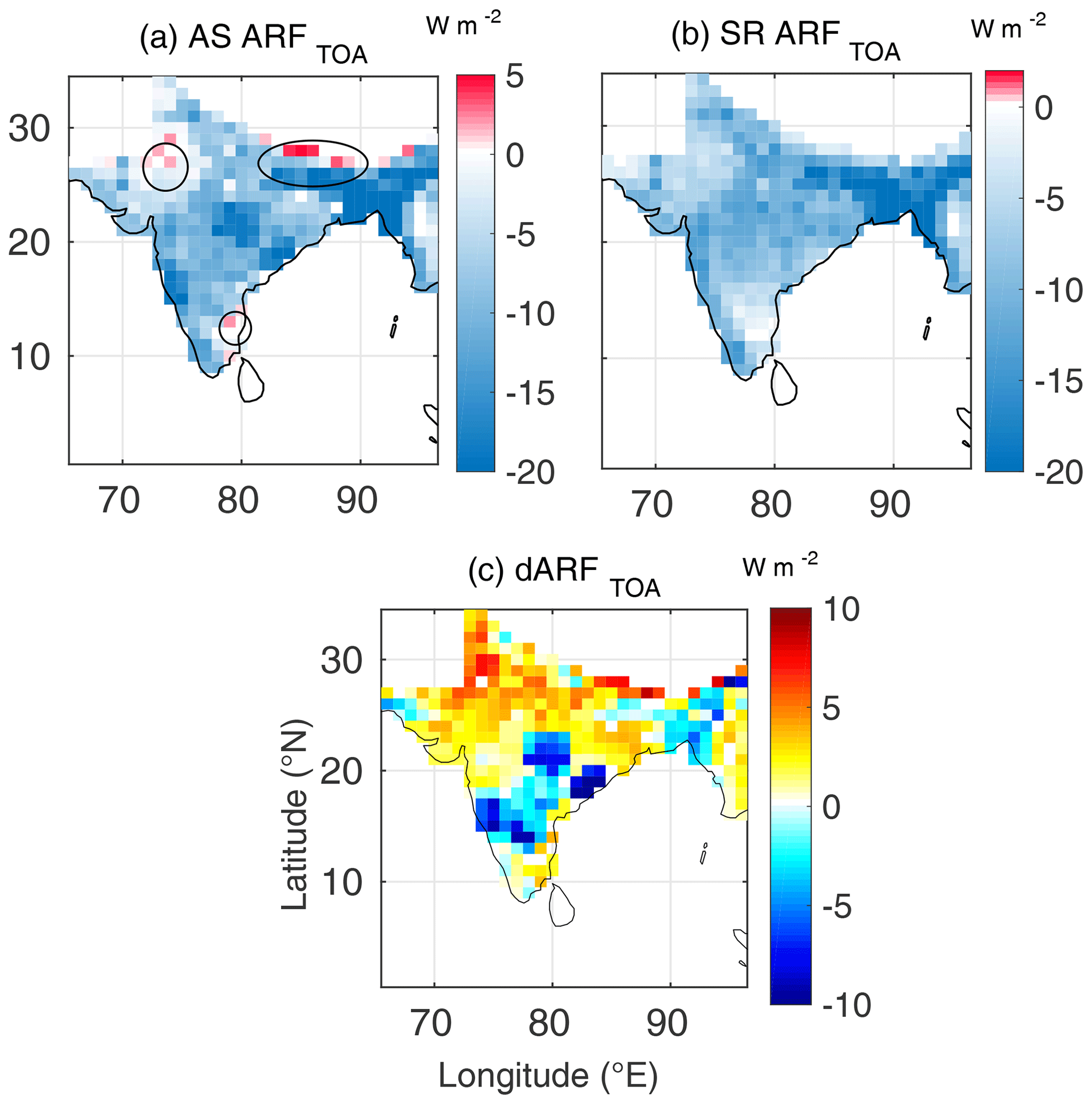
Figure 2 Spatial variation of (a) AS ARF_TOA (radiative forcing estimated using AS AOD and AS SSA, at TOA), (b) SR ARF_TOA (radiative forcing estimated using SR AOD and SR SSA, at TOA) and (c) dARF_TOA for January 2009.

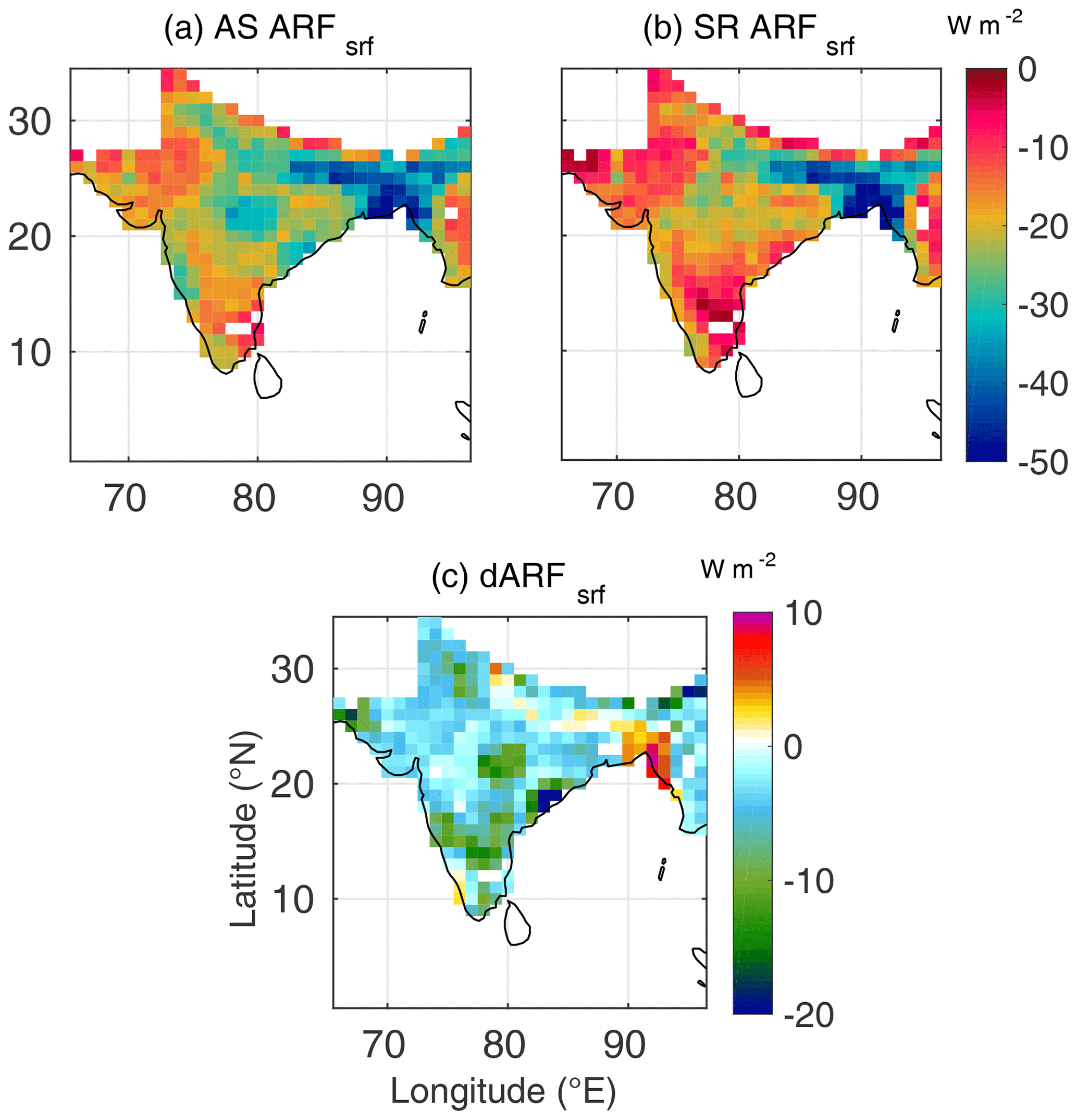
Figure 3 Spatial variation of (a) AS ARF_srf (radiative forcing estimated using AS AOD and AS SSA, at the surface), (b) SR ARF_srf (radiative forcing estimated using SR AOD and SR SSA, at the surface) and (c) dARF_srf for January 2009.

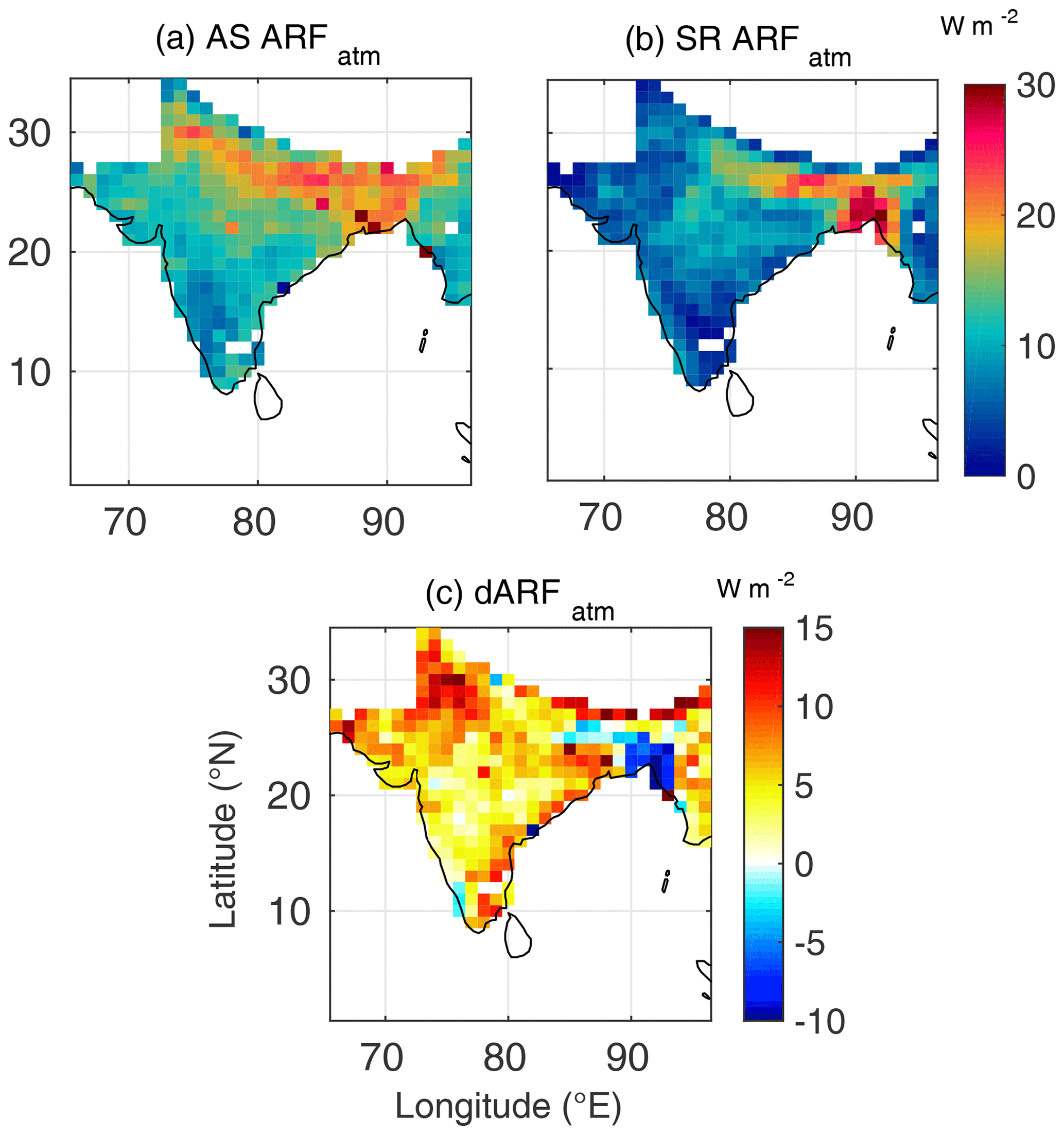
Figure 4 Spatial variation of (a) AS ARF_atm (atmospheric forcing estimated using AS AOD and AS SSA), (b) SR ARF_atm (atmospheric forcing estimated using SR AOD and SR SSA) and (c) dARF_atm for January 2009.

From Figs. 2–4, we can infer the following during winter:

1. Over most of the study domain, ARF estimated using the assimilated datasets shows stronger surface cooling and higher atmospheric warming than that yielded from the satellite-retrieved data, except over outflow region of the Indo-Gangetic Plain. The higher atmospheric forcing when the assimilated dataset is used is mainly contributed by the lower SSA in the assimilated data (due to assimilation with ground-based measurements of aerosol absorption).

2. Over most of the domain, the TOA forcing remains negative in both the estimates, though the magnitude is lower when assimilated data are used. However, weak positive values are seen over the arid regions of the north-west, the Himalayan foothills and a small region on the eastern part of the peninsula (circled in Fig. 2a).

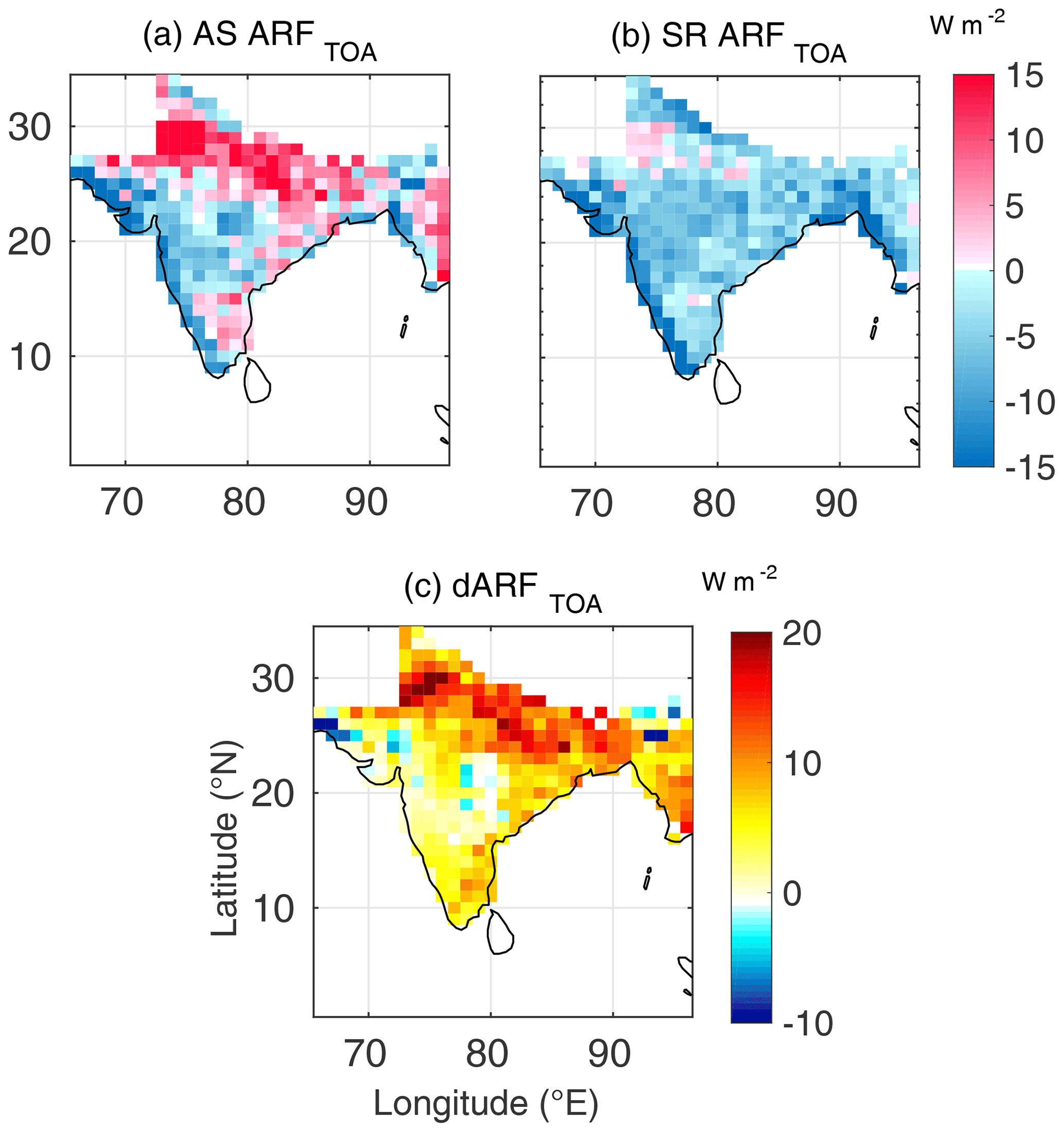
Figure 5 Spatial variation of (a) AS ARF_TOA (radiative forcing estimated using AS AOD and AS SSA, at TOA), (b) SR ARF_TOA (radiative forcing estimated using SR AOD and SR SSA, at TOA) and (c) dARF_TOA for May 2009.

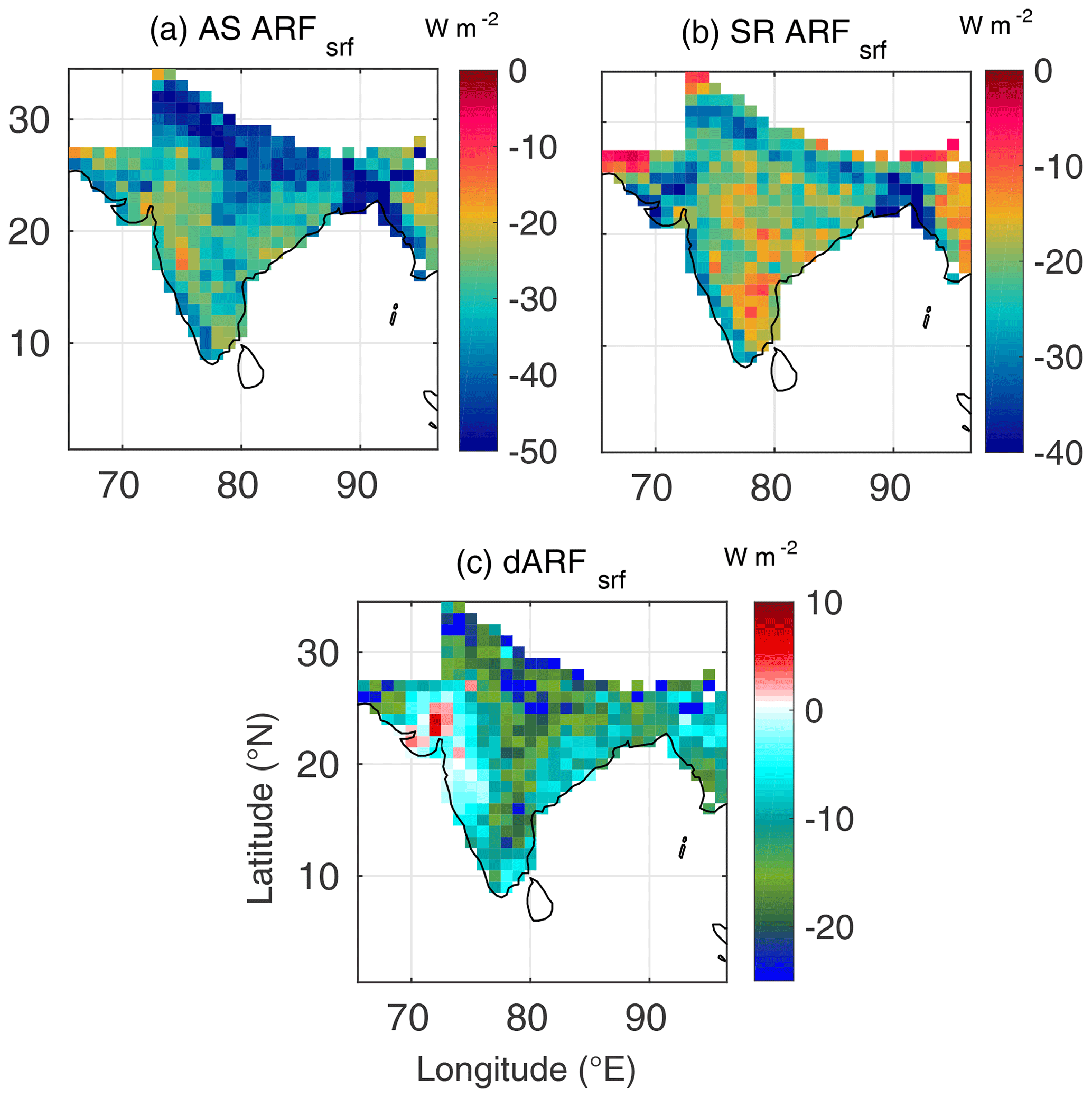
Figure 6 Spatial variation of (a) AS ARF_srf (radiative forcing estimated using AS AOD and AS SSA, at the surface), (b) SR ARF_srf (radiative forcing estimated using SR AOD and SR SSA, at the surface) and (c) dARF_srf for May 2009.

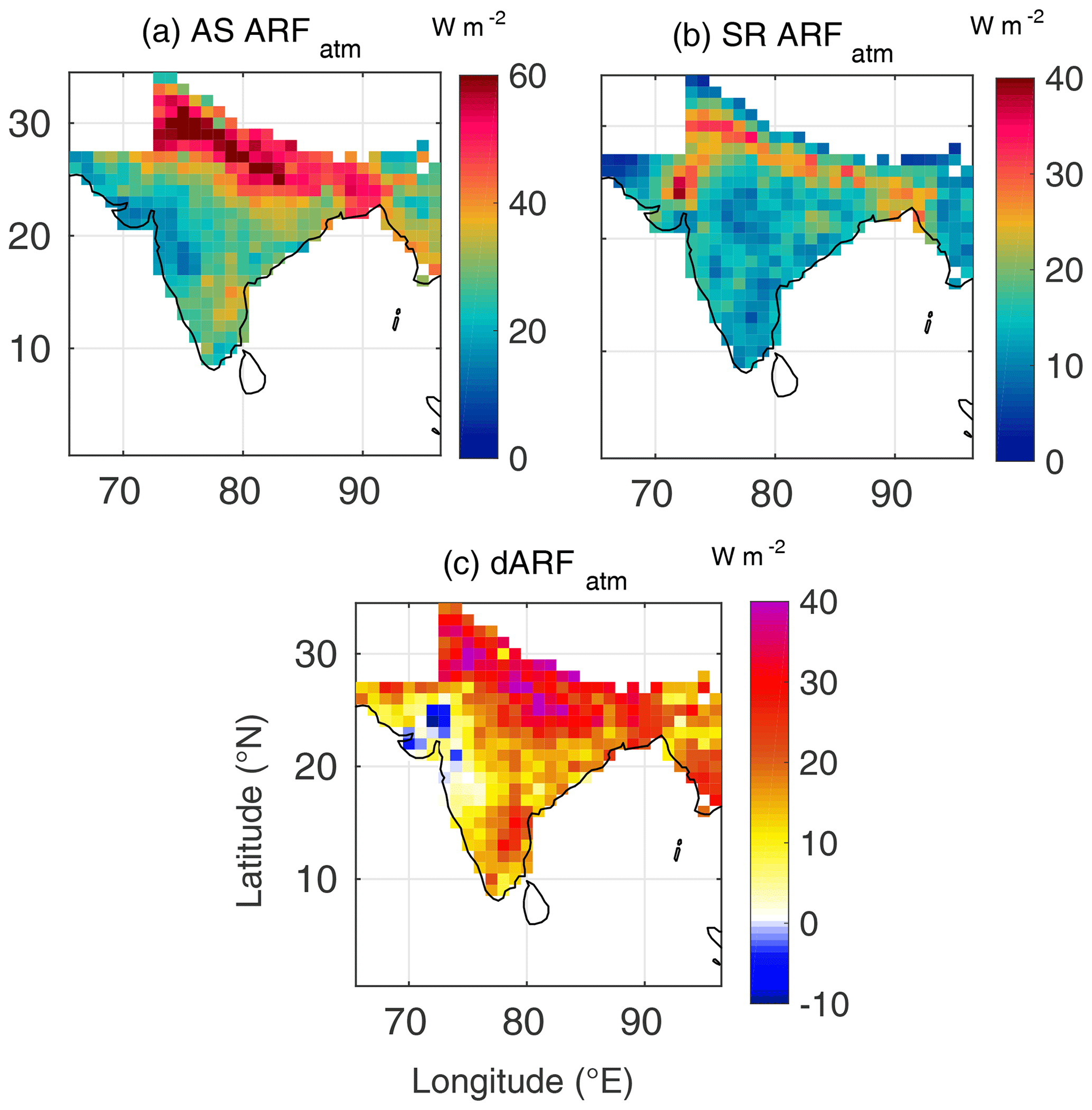
Figure 7 Spatial variation of (a) AS ARF_atm (atmospheric forcing estimated using AS AOD and AS SSA), (b) SR ARF_atm (atmospheric forcing estimated using SR AOD and SR SSA) and (c) dARF_atm for May 2009.

During summer (Figs. 5–7), the seasonal transformation of radiative impacts is clearly seen in the assimilated forcing (mainly due to seasonal change in the aerosol types with anthropogenic aerosols being abundant during winter and natural aerosols during summer). The salient features are as follows:

1. There is a significantly large increase in all the three components of aerosol forcing compared to the wintertime values, primarily due to enhanced aerosol loading in summer.

2. This enhancement is seen more conspicuously in the maps using assimilated data (AOD and SSA) as inputs than those generated using satellite-derived data as input over most parts of the region.

3. In sharp contrast to the winter case, during summer, the TOA forcing using assimilated data shows positive values over a large area, with highest values over the Indo-Gangetic Plain (IGP) and eastern Indian landmass, primarily resulting from incorporation of more realistic values of SSA in the assimilated data. Surface forcing remains, nevertheless, negative in both the estimates.

4. Consequently, higher atmospheric forcing results over the entire landmass, except for a small region in the north-west, when assimilated data are used (Fig. 7c).

5. Positive TOA forcing and strong atmospheric absorption over the IGP results from the presence of absorbing aerosol species, (mainly carbonaceous aerosols and mineral dust; Moorthy et al., 2005; Niranjan et al., 2007; Vaishya et al., 2018), which brings down the SSA, and the respective ground-based measurements reflecting the same are assimilated in the AS datasets (Pathak et al., 2019). The strong and vigorous vertical motions within the convective boundary layers (when the surface temperatures are above 40 ^∘C during large parts of daytime) lift these aerosols to upper levels of the atmosphere (Prijith et al., 2016), thereby further increasing the absorption (Chand et al., 2009). Thus, higher aerosol loading from local as well as remote sources and stronger vertical mixing within deeper planetary boundary layer (especially during pre-monsoon) over the IGP could be responsible for higher ARF over the Indo-Gangetic region vis-à-vis other parts.

   However, it is to be noted here that the actual verification of these features regarding vertical distribution of aerosols and their corresponding effects on ARF at regional level demands vertically resolved, gridded aerosol datasets instead of column-integrated aerosol products. Currently, we are in the process of assimilating the entire dataset from airborne measurements over the Indian regions (Babu et al., 2016; Vaishya et al., 2018), carried out during different campaigns since 2016. The resulting vertically resolved and observationally constrained gridded aerosol properties would be suitable for the regional level assessment of vertical distribution of ARF.

6. The positive TOA forcing values occurring over eastern peninsular India (Figs. 2a and 5a) are primarily due to lower columnar SSA values (0.7 to 0.85) during winter and pre-monsoonal months as demonstrated in Fig. 1d and h, respectively. These low SSA values indicate the increased presence of black carbon (BC) which can be largely associated with large anthropogenic activities. This region has several major harbours, industries and large urban conglomerates such as Chennai (13.08^∘ N, 80.27^∘ E), Vijayawada (16.51^∘ N, 80.65^∘ E), Visakhapatnam (17.68^∘ N, 83.21^∘ E), Bengaluru (12.97^∘ N, 77.59^∘ E) and Bhubaneswar (20.30^∘ N, 85.42^∘ E).

4.2 Comparison with CERES measurements

The above-described spatial distribution of aerosol direct forcing and the large season-dependent differences in between the estimates made using assimilated and satellite-retrieved datasets call for a quantitative verification based on independent measurements, which would delineate the datasets that has better accuracy over the study domain. This exercise would also qualify the superior datasets as inputs to climate models for impact assessment. With a view towards accomplishing this, we have compared the TOA fluxes, estimated using the assimilated and satellite-based datasets with spatiotemporally collocated measurements by CERES aboard the Aqua satellite for clear-sky conditions. CERES is a scanning broadband radiometer which measures the upwelling radiances at TOA over three spectral regimes: the shortwave (0.3–5 µm), the infrared window (8–12 µm) and the total (0.3–200 µm). These measured radiances are then converted into the radiative fluxes using the scene-dependent empirical angular distribution models (Loeb et al., 2003), which are then regridded to $\mathrm{1}{}^{\circ }\times \mathrm{1}{}^{\circ }$ grid. In the present study, we have used the regridded, monthly averaged instantaneous flux measurements at TOA provided by the CERES-SSF (single-scan footprint) product for clear-sky conditions. However, it is to be noted that the root mean square (rms) uncertainty (1σ) corresponding to this monthly averaging of instantaneous shortwave flux measurements is around 9 W m⁻² (over land). In addition, the monthly CERES SW flux measurements also suffer from the uncertainties arising from those in calibration of the CERES instrument (1 W m⁻²) and radiance to flux conversion process (1 W m⁻²; Su et al., 2015).

As the equatorial crossing time (ECT) of Aqua (local solar time for ascending orbit) varies slightly about its mean value of 13:30 LST (local solar time) (Price, 1991; Ignatov et al., 2004), we have estimated the TOA fluxes using the assimilated and satellite-retrieved datasets at time T and T±σ_T, where T is the mean equatorial crossing time and σ_T is the standard deviation in ECTs. The rest of the inputs to SBDART remained the same for the estimates as those given in Sect. 3. The TOA fluxes thus estimated employing assimilated and satellite-based aerosol products are time averaged (over T and T±σ_T) for each month and then compared with monthly mean CERES-measured fluxes. The above-estimated time-averaged fluxes corresponding to assimilated and satellite aerosol products are henceforth, respectively, denoted as AS RAD_TOA and SR RAD_TOA, and respective CERES flux measurements are referred to as CERES_TOA. With a view towards quantifying the comparisons, we have computed the deviations of AS RAD_TOA and SR RAD_TOA from corresponding CERES measurements for each month during the period of 5 years (2009–2013)(excluding the monsoon months of JJAS, due to extensive cloud cover).

$$\begin{array}{}\text{(7)}& {\displaystyle }{\mathit{\delta }}_{\mathrm{AS}}=\mathrm{AS}{\mathrm{RAD}}_{\mathrm{TOA}}-{\mathrm{CERES}}_{\mathrm{TOA}}\text{(8)}& {\displaystyle }{\mathit{\delta }}_{\mathrm{SR}}=\mathrm{SR}{\mathrm{RAD}}_{\mathrm{TOA}}-{\mathrm{CERES}}_{\mathrm{TOA}}\end{array}$$

In Eq. (7) (Eq. 8) above, δ_AS (δ_SR) denotes deviations in the absolute magnitudes of TOA fluxes estimated employing assimilated (satellite-retrieved) datasets from the corresponding CERES-measured fluxes. Accordingly, positive values of δ_AS (δ_SR) imply higher magnitudes of the TOA fluxes estimated using the assimilated (satellite) datasets vis-à-vis CERES measurements. The monthly time series of the rms of flux deviations (δ_AS, δ_SR) are presented in Fig. 8 in the form of box-and-whisker plots, for the entire study period (referred to as “annual”) as well as for the following three seasons: pre-monsoon (PrM; March–April–May; MAM), winter (December–January–February; DJF) and post-monsoon (PoM; October–November; ON).

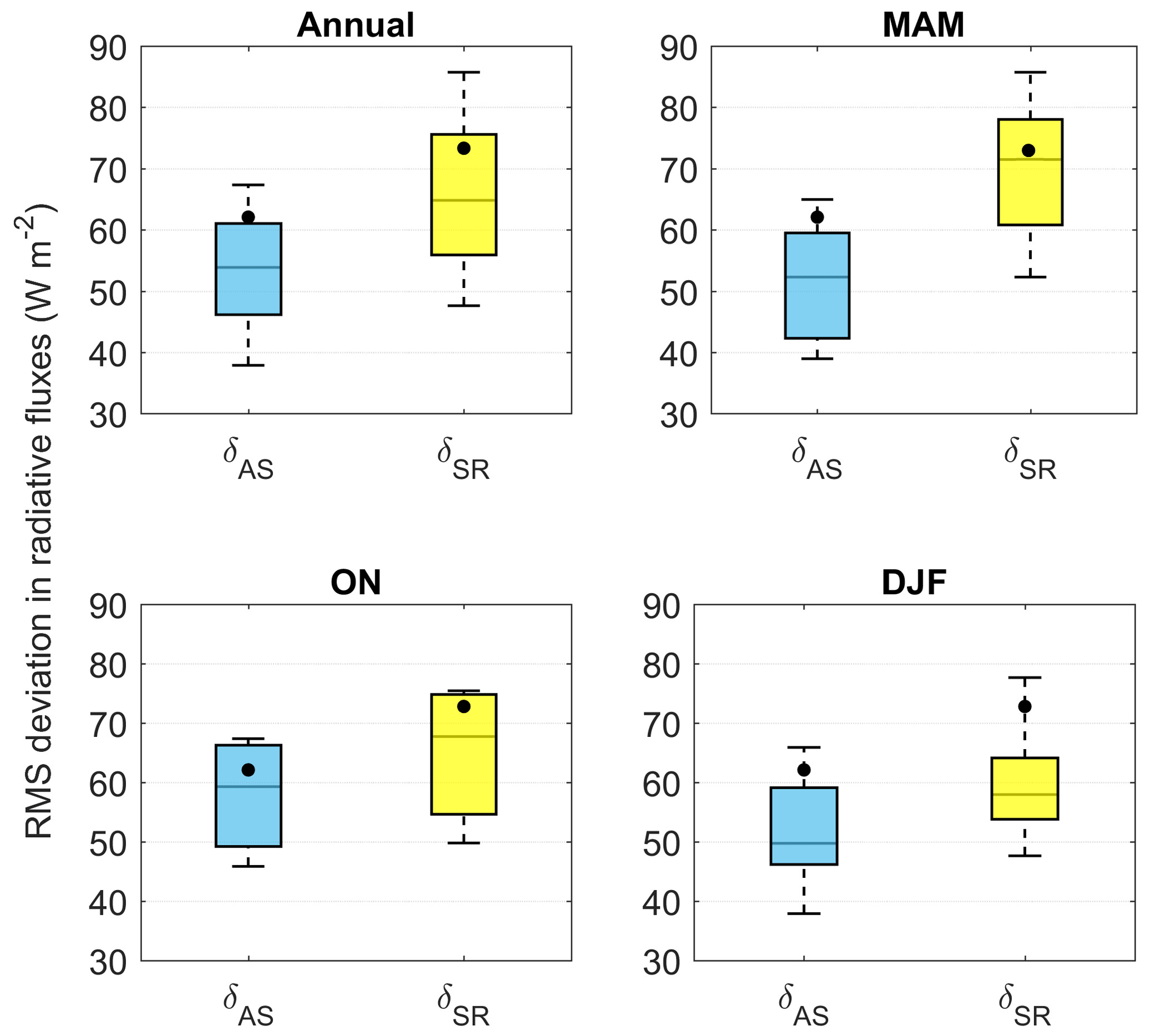
Figure 8 Box-and-whisker plots for monthly rms(δ_AS) (blue coloured box) and rms(δ_SR) (yellow coloured box) for the duration of 2009–2013. The bottom and top ends of the boxes, respectively, denote the 25th and 75th percentiles, the median is denoted by the black horizontal line within each box, and the black circle represents the mean of the respective population.

Figure 8 unequivocally shows that median and mean of flux deviations are substantially smaller (at 95 % confidence level) for estimates made using the assimilated datasets than when the satellite-retrieved datasets are used for all the seasons as well as for the entire monthly time series represented by the annual case. However, the difference between the two distributions (δ_AS, δ_SR) is more conspicuous during the MAM season (Fig. 8), which is the season of intense aerosol loading over this domain, due to the combined actions of local emissions and long-range transport being thoroughly mixed and vertically lofted by strong thermal convections. This quantifies the better accuracy of the observationally constrained, assimilated, gridded aerosol products over the satellite-retrieved aerosol products, over the study domain for inputting in ARF estimation.

Table 1 Annual and seasonal mean CERES TOA flux measurements and difference between AS RAD_TOA and CERES_TOA in W m⁻².

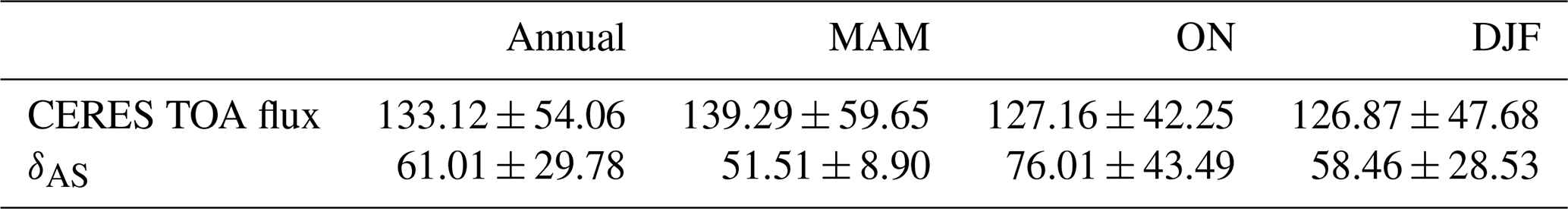
However, there are significant differences between TOA fluxes estimated using assimilated products and CERES measurements (∼40 to 70 W m⁻² for the annual case; Fig. 8a). The annual and seasonal mean values of these differences (rms, δ_AS) and the corresponding CERES_TOA measurements are provided the Table 1. It is to be noted that the standard deviation values provided in the Table 1 correspond to annual and seasonal averaging of respective variables over the domain and are representative of the statistical variations.

These differences (δ_AS) would arise from the uncertainties and biases in AS RAD_TOA and CERES_TOA. However, being constructed from high-quality direct ground-based measurements (Pathak et al., 2019), the systematic bias in the assimilated aerosol properties and hence in AS RAD_TOA tends to be very small. Therefore, the δ_AS values reported in Fig. 8 and Table 1 would primarily be due to random errors in AS RAD_TOA and CERES_TOA. In the view of this, we have estimated the uncertainties in AS RAD_TOA which primarily originate from those in assimilated AOD and SSA as well as from averaging of AS RAD_TOA over the Aqua satellite crossing duration. The uncertainties in AS RAD_TOA due to those in assimilated aerosol products are estimated following the procedure similar to that explained in Appendix A for the two representative cases of January and May 2009, and the typical value of rms uncertainty (1σ) in AS RAD_TOA is around 5.8 W m⁻². Further, the rms uncertainty (1σ) due to temporal averaging of AS RAD_TOA over the duration corresponding to expected variation in the satellite crossing time is observed to be 7.6 W m⁻². The uncertainties in instantaneous TOA flux measurements provided by CERES-SSF (monthly averaged) are already described above.

It can be seen from the above discussion and the Table 1 that the estimated rms difference between the AS RAD_TOA and CERES_TOA (i.e. δ_AS which varies from ∼ 40 to 70 W m ⁻² for annual mean case) is substantially contributed by the uncertainties in AS RAD_TOA and CERES_TOA. In addition, the uncertainties associated with MODIS surface reflectance products and the assumed aerosol phase function would also contribute to those in the AS RAD_TOA and would reflect in rms (δ_AS). It is to be noted here that although the assimilated aerosol products have demonstrated much better confirmation with independent ground-based direct measurements (Pathak et al., 2019) vis-à-vis satellite-based products, over regions where the ground-based measurements are less dense or sparse, they would tend to be very close to or nearly the same as their satellite counterparts which suffer from substantial uncertainties and biases (Zhang and Reid, 2006; Jethva et al., 2014, 2009) as discussed in Pathak et al. (2019) (the Part 1 paper). As such, to further reduce the differences between the model-estimated (using assimilated products) and CERES-measured TOA fluxes, it is required to have denser network of ground-based aerosol measurements. In addition, incorporating spatiotemporally varying aerosol phase function datasets and vertical profiles of aerosol extinction and SSA is expected to reduce the differences between the estimated and measured TOA flux measurements further.

This analysis establishes the improved effectiveness of TOA fluxes estimated using assimilated vis-à-vis satellite products and the similar improvement is implied in the ARF corresponding to assimilated aerosol products than those estimated using their satellite counterparts. In the view of this, we have performed the regional level estimation of the aerosol-induced atmospheric heating rate (columnar) using the atmospheric absorption corresponding to assimilated aerosol datasets and compared it to those estimated using satellite aerosol products.

4.3 Atmospheric heating rate estimation

The atmospheric forcing component of ARF is the amount of energy absorbed by the atmosphere, which heats the atmosphere. The heating rate due to aerosol-induced atmospheric absorption is calculated as shown in Eq. (9).

$$\begin{array}{}\text{(9)}& {\displaystyle \frac{\partial T}{\partial t}}={\displaystyle \frac{g}{C_p}}{\displaystyle \frac{\mathrm{\Delta }F}{\mathrm{\Delta }P}}\end{array}$$

Here, $\frac{\partial T}{\partial t}$ is the atmospheric heating rate (K S⁻¹), g is the acceleration due to gravity, C_p is the specific heat of air at constant pressure (∼1005 J kg⁻¹ K⁻¹), ΔF is the aerosol-induced atmospheric absorption, and P is the atmospheric pressure. Here, ΔP is considered to be 300 hPa (pressure varying from 1000 to 700 hPa) implying that atmospheric aerosols are largely concentrated in the first 3 km above the ground, which is also supported by observations (Parameswaran et al., 1995; Müller et al., 2001).

The spatial distribution of diurnally averaged atmospheric heating rates estimated using assimilated datasets (HR_AS) and its difference from similar estimates made using satellite-retrieved aerosol datasets (HR_AS−HR_SR) are shown in Fig. 9 for two representative months (January and May 2009).

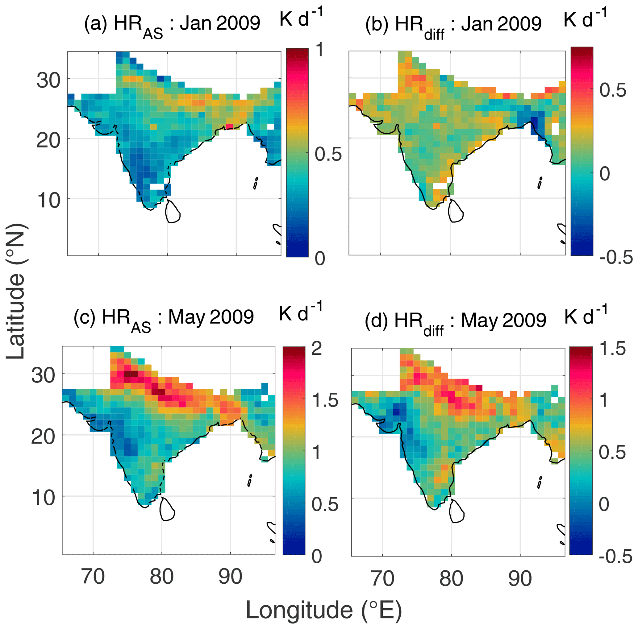
Figure 9 Spatial variation of aerosol-induced atmospheric heating rate (in K d⁻¹) estimated using assimilated aerosol products (HR_AS) for January and May 2009 (a and c, respectively), difference between aerosol-induced atmospheric heating rate corresponding to assimilated and satellite aerosol products (HR${}_{\mathrm{diff}}={\mathrm{HR}}_{\mathrm{AS}}-{\mathrm{HR}}_{\mathrm{SR}}$) for January and May 2009 (b and d, respectively).

The figure reveals consistently higher heating rates (∼0.6 to 0.7 K d⁻¹ during January 2009 and ∼1.5 to 2.0 K d⁻¹ during May) over the IGP than the rest of the subregions. As indicated by positive values of HR_diff, the heating rate estimates using assimilated datasets are consistently higher than those estimated using satellite-derived aerosol products. Further examination of Fig. 9 reveals that there is significant seasonality in the atmospheric heating rate, with pre-monsoonal month (May) exhibiting substantially stronger warming than that during the winter month of January, over most of the Indian region. In view of this, we have examined the seasonal variation in the aerosol radiative forcing over the Indian region in the next section.

4.4 Seasonal and subregional features

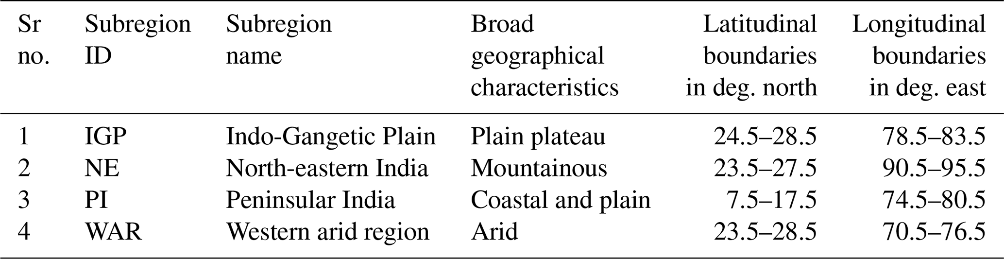
Aerosol types and their properties over the Indian region are known to exhibit significant seasonal variation, both at regional and subregional scales, primarily due to seasonality in the nature of aerosol sources, advection pathways as well as synoptic and mesoscale meteorology (Jethva et al., 2014; Krishna Moorthy et al., 2007; Babu et al., 2013; Vaishya et al., 2018; Pathak et al., 2019). We examine the signatures of these in direct ARF. For this analysis, we have considered four subregions of the spatial domain based on the homogeneity of broad-scale geographical features as detailed in Fig. 10 and Table 2.

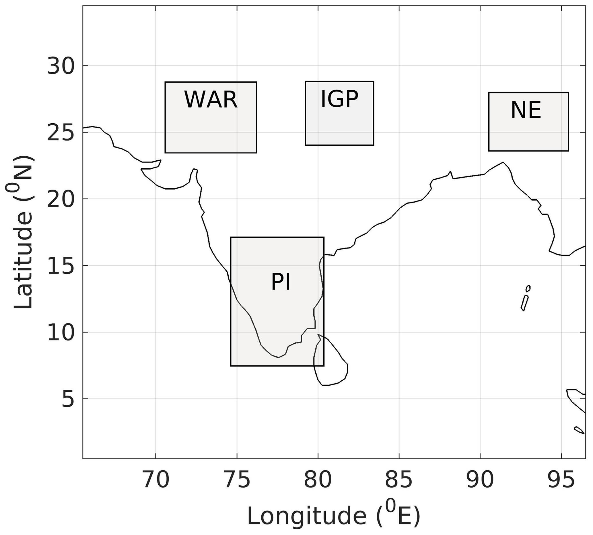
Figure 10 Subregions of the spatial domain.

Table 2 Details of subregions considered.

The climatological seasonal variation of TOA forcing and atmospheric absorption estimated employing assimilated aerosol products and averaged over four subregions are presented in Figs. 11 and 12, respectively, with panels a–d in each figure, respectively, representing the IGP, NE, PI and WAR. Please note that the vertical lines over the bars in Figs. 11 and 12 indicate the spatiotemporal variation in ARF over the respective subregion and not the uncertainties in radiative forcing.

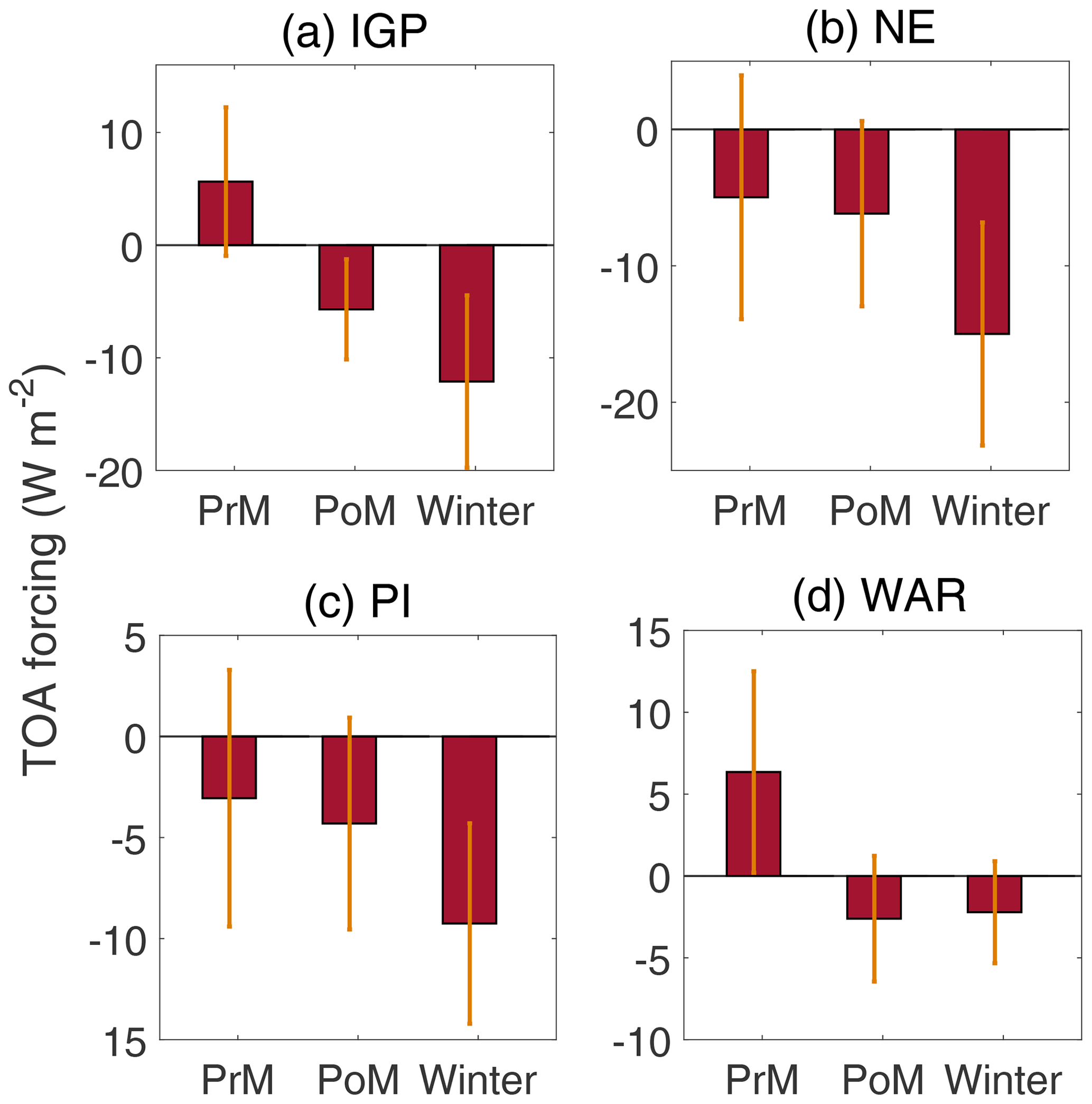
Figure 11 The climatological seasonal variation of aerosol radiative forcing at TOA estimated using assimilated aerosol products and averaged over four subregions: (a) IGP, (b) NE, (c) PI and (d) WAR.

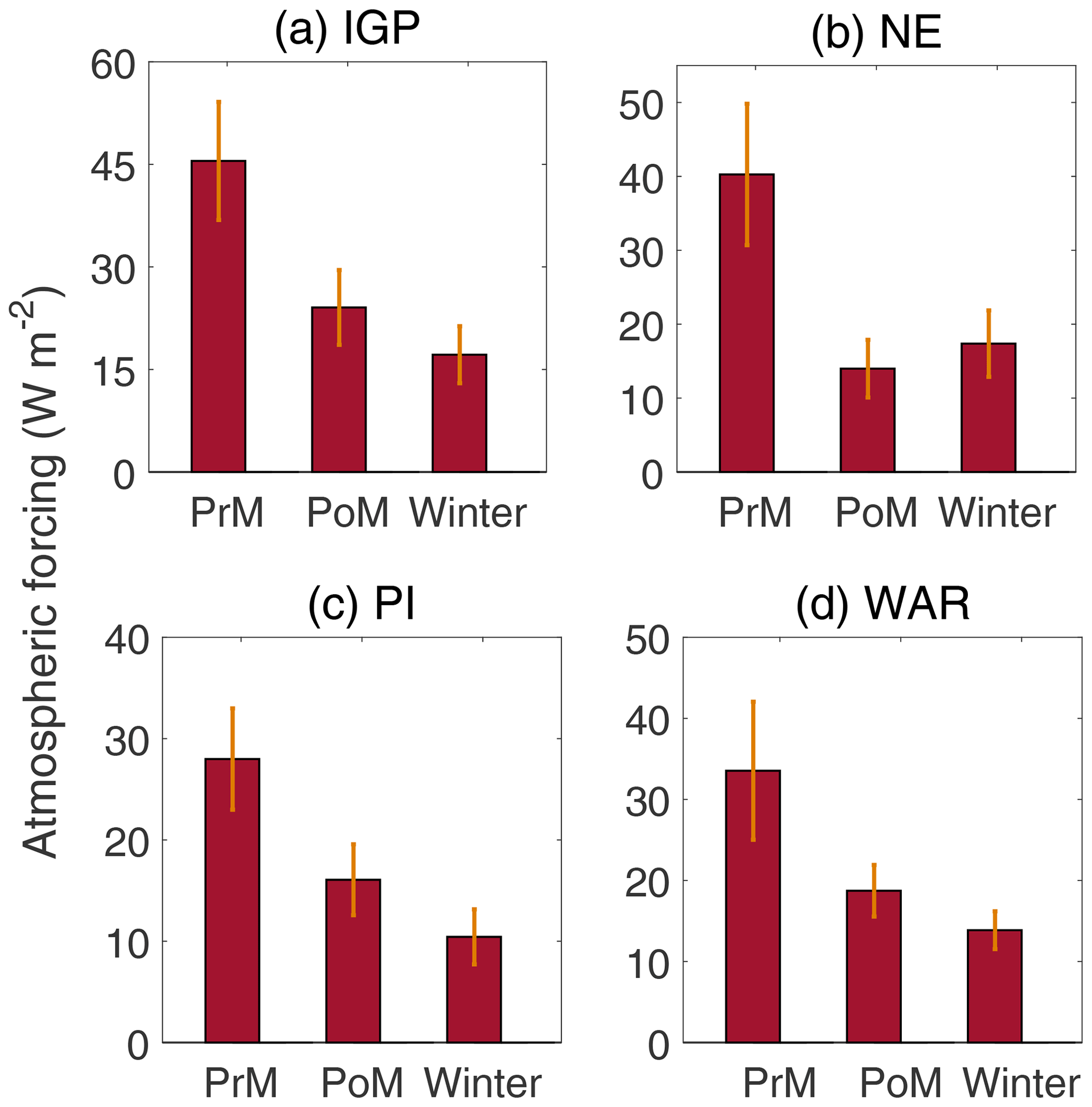
Figure 12 The climatological seasonal variation of atmospheric absorption due to aerosols estimated using assimilated aerosol products and averaged over four subregions: (a) IGP, (b) NE, (c) PI and (d) WAR.

Figure 11 clearly demonstrates the following:

1. The TOA forcing is mostly negative over all the subregions and most of the seasons, except over the two subregions (IGP and WAR), which are highly influenced by advected and locally emitted dust (Banerjee et al., 2019) during pre-monsoon seasons.

2. Seasonally, the magnitude of TOA forcing is highest during winter and lowest during pre-monsoon over most of the subregions, except WAR (Fig. 11d) for which the highest magnitude of TOA forcing occurs during pre-monsoon and lowest during winter, again primarily due to the influence of mineral dust.

Almost in agreement with the TOA forcing, atmospheric absorption (Fig. 12) is at maximum during pre-monsoon (when TOA forcing is minimum negative) and least during winter (when TOA forcing is maximum negative) over most of the subregions, except the NE subregion (Fig. 12b), which shows the lowest atmospheric absorption during post-monsoon. The highest values of atmospheric forcing though appear over the IGP (Fig. 12a) and lowest over PI (Fig. 12c).

Further, we have estimated the uncertainties in the ARF estimated using assimilated as well as satellite aerosol products and the exercise revealed that the uncertainties in AS ARF are substantially smaller than those in SR ARF, which is a direct consequence of smaller uncertainties in assimilated AOD and SSA vis-à-vis respective satellite products (Pathak et al., 2019). The corresponding details are provided in Appendix A.

5 Summary

We have estimated shortwave, clear-sky direct aerosol radiative forcing over the Indian region by incorporating gridded, assimilated, multi-year (2009–2013) datasets for monthly AOD and SSA in SBDART and compared its spatiotemporal features with those in ARF estimated using presently available satellite-retrieved aerosol products. This work is the first of its kind over the Indian region that computes regional ARF estimates that employ assimilated, gridded datasets constrained by highly accurate aerosol measurements performed with a dense network of ground-based observatories spanning across the Indian region. In order to examine the accuracy of these ARF estimates, the monthly instantaneous TOA fluxes estimated using assimilated and satellite-retrieved products are compared against the monthly averaged, instantaneous CERES measurements. Finally, we have estimated the aerosol-induced atmospheric warming rates and discussed their spatiotemporal features. The primary findings of the present work are as follows:

1. The TOA fluxes estimated using the assimilated datasets conform better with independent and concurrent space-borne measurements performed by CERES as compared to those shown by TOA fluxes corresponding to satellite-retrieved datasets. This establishes the higher accuracy of ARF estimated using assimilated vis-à-vis satellite aerosol products.

2. The diurnally averaged ARF corresponding to assimilated aerosol properties depicts significant spatial and temporal diversity not only in terms of the magnitudes but also in the sign of ARF at TOA. The Indo-Gangetic Plain, north-eastern parts and southern parts of peninsular India exhibit either negative forcing with smaller magnitudes or positive forcing, as compared to rest of the region, demonstrating negative TOA forcing of relatively larger magnitudes.

3. The regional distribution of radiative forcing also reveals increased surface cooling and atmospheric absorption over the Indo-Gangetic Plain and arid regions from north-western India vis-à-vis rest of the region.

4. Similar large-scale spatial features are also shown by ARF estimated using satellite products; however, they differ from their assimilated counterparts in terms of magnitude as well as sign of TOA forcing.

5. In consonance with the aerosol-induced atmospheric forcing, the atmospheric warming rates exhibit significant spatial heterogeneity (∼0.2 to 2.0 K d⁻¹), with the Indo-Gangetic region demonstrating largest values (∼ 0.6 to 2.0 K d⁻¹). In most of the cases, the heating rates corresponding to assimilated products demonstrate substantially increased lower-tropospheric warming vis-à-vis those corresponding to satellite aerosol products.

6. Over most parts of the region, the TOA forcing is negative throughout the year, with maximum magnitudes occurring during winter and minimum during pre-monsoon, except the Indo-Gangetic Plain and western arid regions over which the sign of TOA forcing flips from positive (during pre-monsoon) to negative (during post-monsoon and winter). However, the atmospheric forcing due to aerosols is highest during pre-monsoon and lowest during winter over almost the entire Indian region.

7. The uncertainties in ARF estimated using assimilated aerosol products are substantially lower than those in ARF estimated using satellite products, which is a natural consequence of smaller uncertainties in assimilated vis-à-vis satellite aerosol products.

On the background of these benefits, the present ARF estimates and the corresponding assimilated aerosol products can be potentially applied for improving the accuracy of aerosol climate impact assessment at regional, subregional and seasonal scales.

Appendix A: Uncertainties in ARF

One of the prime challenges in the accurate climate impact assessment of aerosols is posed by the uncertainties in the estimation of direct aerosol radiative effect. These uncertainties primarily emanate from those in the gridded datasets for aerosol properties, mainly AOD and SSA. Past studies have shown that small changes in SSA can even change the sign of aerosol radiative forcing at TOA (Haywood and Shine, 1995, 1997; Heintzenberg et al., 1997; Russell et al., 2000; Takemura et al., 2002; Loeb and Su, 2010; Babu et al., 2016). Against this backdrop, it becomes imperative to assess the uncertainties in the radiative forcing estimates presented in the current study.

For estimation of uncertainties in aerosol radiative forcing, we have derived multiple realizations of diurnally averaged ARF (at TOA, surface and within the atmosphere) at each grid point over the Indian region, with each of these ARF realizations corresponding to a particular AOD and SSA which are perturbed from the original values within their respective uncertainty limits. The uncertainties in assimilated AOD and SSA are estimated as discussed in Part 1 of the two-part paper (Pathak et al., 2019). The uncertainties in SR AOD (which is largely comprised of MODIS AODs) are estimated as $\pm (\mathrm{0.03}+\mathrm{0.2}{\mathit{\tau }}_{\mathrm{M}})$ (Sayer et al., 2013) where τ_M is the corresponding MODIS AOD. The uncertainty in OMI SSA is considered to be ±0.05 following Jethva et al. (2014). For a given grid point, the standard deviation across the multiple realizations of ARF is then considered to be the uncertainty in the radiative forcing estimate. Thus, we have estimated the uncertainties in ARF corresponding to assimilated and satellite-based aerosol products.

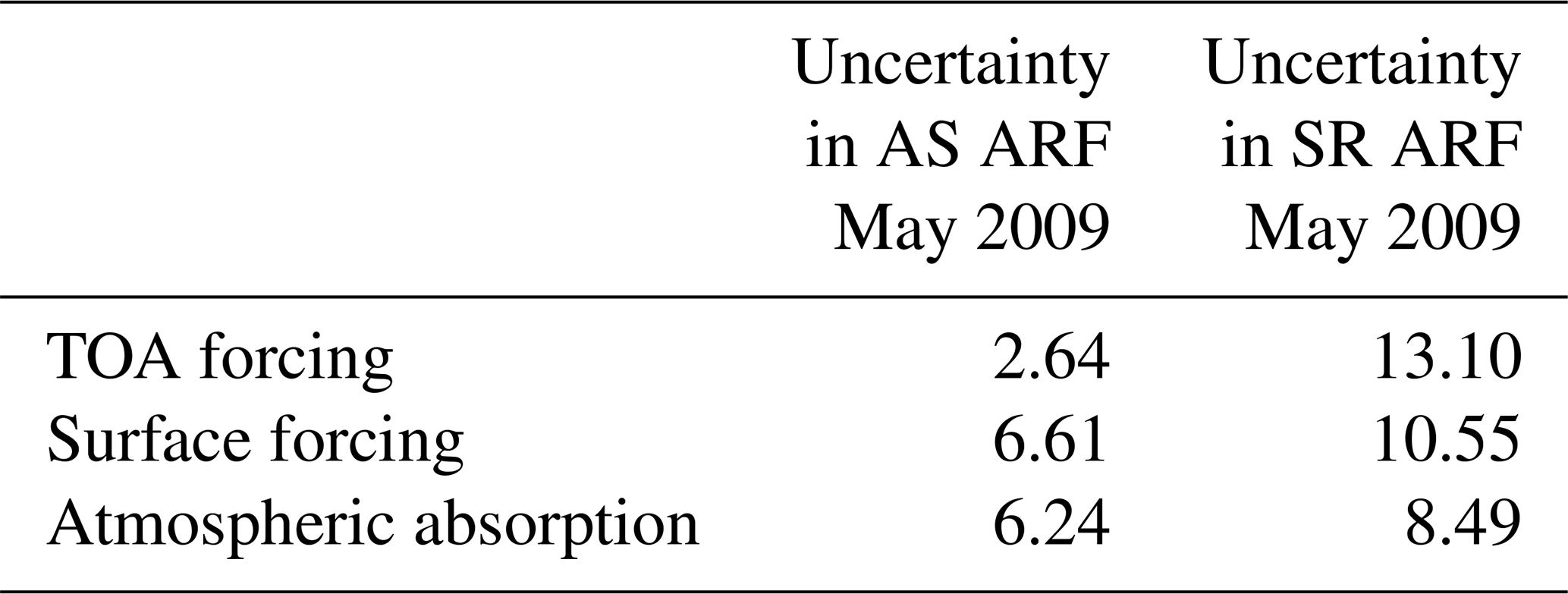
The rms uncertainties in the ARF at TOA, surface and atmospheric absorption estimated using assimilated aerosol products are presented and compared with those in ARF estimated using satellite-derived aerosol products in Tables A1 and A2, for the two representative months, January and May 2009, respectively.

Tables A1 and A2 demonstrate that uncertainties in AS ARF are substantially smaller than those in SR ARF, which is the consequence of smaller uncertainties in assimilated aerosol products as compared their satellite counterparts. It can further be seen from Tables A1 and A2 that uncertainties in aerosol radiative forcing estimated using assimilated datasets are smallest for the forcing at TOA as compared to surface forcing and atmospheric absorption. This is in contrast with the ARF corresponding to satellite products for which the TOA forcing exhibits the highest uncertainty vis-à-vis its surface and atmospheric counterparts, which is in line with Chung et al. (2005), in which the global mean TOA forcing (estimated using assimilated product having a quite limited signature of ground-based aerosol data) is demonstrated to have higher uncertainties than those in surface and atmospheric forcing. Further inspection of Tables A1 and A2 reveals that uncertainties in AS ARF during May 2009 are smaller than those during January 2009. This could be primarily because of the assimilated aerosol datasets for May 2009 assimilating high-quality aerosol measurements from a greater number of stations (19 stations each for AOD and absorption AOD (AAOD) assimilation) vis-à-vis January 2009 (17 and 15 stations for AOD and AAOD assimilation, respectively) leading to reduced uncertainties in assimilated AOD and SSA during May compared to January 2009 and the consequential effect on uncertainties in AS ARF.

Table A1 The rms uncertainty in direct aerosol radiative forcing over the Indian region for January 2009.

Table A2 The rms uncertainty in direct aerosol radiative forcing over the Indian region for May 2009.

Unlike AOD and SSA, there are no extensive ground-based and/or airborne measurements of aerosol size distributions to generate gridded datasets available for estimating the aerosol phase function. As such, we have used phase functions corresponding to appropriate aerosol models from the Optical Properties of Aerosols and Clouds (OPAC; Hess et al., 1998) in order to estimate ARF using SBDART. The estimated rms uncertainties are around 2.2 % (1σ) across the eight streams of Legendre moments used in the radiative transfer model. While AOD and SSA are the biggest contributing factors while estimating ARF, phase function plays a relatively less significant role as ARF is the integrated effect over the hemisphere (not angular).

In order to estimate the sensitivity of ARF estimates to the expected variations in the above aerosol phase function, we have simulated the ARF (at TOA, the surface and within the atmosphere) for the representative month of January 2009, over the entire Indian region. Each of these simulations was carried out by incorporating Legendre moments of aerosol phase function corresponding to each of the continental aerosol models provided in OPAC along with columnar, assimilated AOD and SSA in SBDART. The uncertainty of ARF with regard to that phase function is then estimated as 1 standard deviation across the multiple ARF simulations. This analysis has revealed that the rms uncertainty (1σ) in ARF at TOA, surface and in the atmosphere is around 4 %, 0.22 % and 0.05 %, respectively. This analysis shows that the present ARF estimates corresponding to assimilated aerosol products are substantially robust with regard to expected variations in aerosol phase function; however, further improvement in accuracies of the ARF estimation will be possible when realistic size distribution data are generated in the future.