Wildfire smoke in the lower stratosphere identified by in situ CO observations

Wildfires emit large quantities of aerosols and trace gases, which occasionally reach the lower stratosphere. In August 2017, several pyro-cumulonimbus events injected a large amount of smoke into the stratosphere, observed by lidar and satellites. Satellite observations are in general the main method of detecting these events since in situ aircraft- or balloon-based measurements of atmospheric composition at higher altitudes are not made frequently enough. This work presents accidental balloon-borne trace gas observations of wildfire smoke in the lower stratosphere, identified by enhanced CO mole fractions at approximately 13.6 km. In addition to CO mole fractions, CO₂ mole fractions and isotopic composition of CO (δ¹³C and δ¹⁸O) have been measured in air samples, from both the wildfire plume and background, collected using an AirCore and a lightweight stratospheric air sampler (LISA) flown on a weather balloon from Sodankylä (4–7 September 2017; 67.37^∘ N, 26.63^∘ E; 179 m a.m.s.l.), Finland. The greenhouse gas enhancement ratio (ΔCO:ΔCO₂) and the isotopic signature based on δ¹³C(CO) and δ¹⁸O(CO) independently identify wildfire emissions as the source of the stratospheric CO enhancement. Back-trajectory analysis was performed with the Chemical Lagrangian Model of the Stratosphere (CLaMS), tracing the smoke's origin to wildfires in British Columbia with an injection date of 12 August 2017. The trajectories are corrected for vertical displacement due to heating of the wildfire aerosols, by observations made by the Cloud-Aerosol Lidar with Orthogonal Polarization (CALIOP) instrument. Knowledge of the age of the smoke allowed for a correction of the enhancement ratio, ΔCO:ΔCO₂, for the chemical removal of CO by OH. The stable isotope observations were used to estimate the amount of tropospheric air in the plume at the time of observation to be about 45±21 %. Finally, the plume extended over 1 km in altitude, as inferred from the observations.

1 Introduction

Wildfires emit a large quantity of polluting trace gases and aerosols into the atmosphere (Crutzen and Andreae, 1990; Andreae, 2019). These trace gases and aerosols affect the radiative transfer properties of the atmosphere and lead to the formation of tropospheric ozone. Not only the troposphere is affected, but the smoke also occasionally reaches the lower stratosphere (Waibel et al., 1999; Fromm et al., 2000; Fromm and Servranckx, 2003; Jost et al., 2004; Fromm et al., 2010), enhancing aerosol levels and ozone (Fromm et al., 2005), with potential global effects (Peterson et al., 2018).

In 2017, a large smoke plume in the stratosphere was observed on several days between 24 August and 26 September by ground-based lidar and the Cloud-Aerosol Lidar with Orthogonal Polarization (CALIOP) aboard the CALIPSO satellite (Khaykin et al., 2018). This smoke was attributed to Canadian forest fires, injected by pyro-cumulonimbus (pyro-Cb) events. The cumulative smoke mass injected into the stratosphere by five distinct pyro-Cb events was estimated to be 0.1 to 0.3 Tg (Peterson et al., 2018). The smoke mass density was further characterized using the Aerosol Robotic Network (AERONET) and Moderate Resolution Imaging Spectroradiometer (MODIS; Ansmann et al., 2018), and the micro physical properties of the smoke were determined by lidar studies (Haarig et al., 2018; Hu et al., 2019; Baars et al., 2019).

Past injections of wildfire smoke into the stratosphere were mainly identified and characterized using satellite observations (e.g. Fromm et al., 2010). Nevertheless, wildfire smoke has been observed from in situ aircraft measurements as well. First, Waibel et al. (1999) reported a CO plume in the Northern Hemisphere (NH) extratropical lowermost stratosphere at 10 km altitude. The plume was associated with the extensive 1994 burning season. In addition, Hudson et al. (2004), Ray et al. (2004), and Jost et al. (2004) found several smoke layers between 14.7 and 15.8 km (θ=368 to 393 K). The enhanced levels of CO, up to 193 ppb, were found in the NH subtropical lower stratosphere (25^∘ N), which was 1.3 km above the local tropopause. They attributed the origin of the smoke to North American forest fires. Finally, Cammas et al. (2009) reported on the injection of a smoke plume into the stratosphere also associated with North American forest fires.

In situ observations of wildfire smoke are typically identified by an increase in mole fractions of CO (Waibel et al., 1999; Jost et al., 2004; Cammas et al., 2009). In addition to CO, Cammas et al. (2009) measured O₃, NO_x, and PAN. These measurements correlate well with CO and are thus additional tracers for wildfire smoke. Furthermore, Hudson et al. (2004) and Jost et al. (2004) measured particle mass spectra containing carbon, potassium, organics, and ammonium ions. The stratospheric particle mass spectra were compared to mass spectra obtained from direct smoke measurements in the troposphere (Hudson et al., 2004), confirming the presence of smoke in the stratosphere.

Wildfire smoke has distinct trace gas source signatures. One way to identify the source of smoke is by using the enhancement ratio of ΔCO:ΔCO₂ (Mauzerall et al., 1998), and another way is to use the stable isotopic composition of CO (Brenninkmeijer et al., 1999; Kato et al., 1999; Röckmann et al., 2002). Of the stratospheric observations, only Jost et al. (2004) measured CO₂, allowing ΔCO:ΔCO₂ to be quantified, confirming the smoke's origin. These source signatures have been successfully used in many ground-based and airborne studies on wildfire smoke plumes in the troposphere (e.g. Andreae et al., 2001; Bergamaschi et al., 1998; Tarasova et al., 2007).

This work presents the first balloon-borne CO and CO₂ observation of a wildfire smoke plume in the stratosphere. The AirCore sampling technique (Karion et al., 2010; Membrive et al., 2017) provides an accurate measurement of enhancement ratios of ΔCO:ΔCO₂, where the lightweight stratospheric air sampler (LISA; Hooghiem et al., 2018) is used to collect larger samples that allow for the determination of the carbon and oxygen stable isotopic compositions of CO. A back-trajectory analysis was performed using the Chemistry Lagrangian Model of the Stratosphere, CLaMS (McKenna et al., 2002) to determine the source region and injection date, which helps in the quantification of the chemical loss of CO by OH. The trace gas and isotopic composition measurements are used to confirm the wildfire smoke as origin of the plume. Finally the observations are used to estimate the fraction of tropospheric air in the enhanced smoke plume.

2 Methods

2.1 Sampling instruments and flights

The air sampling was done with LISA (Hooghiem et al., 2018) and an AirCore (Karion et al., 2010). Both instruments are capable of sampling the stratosphere and can be flown using small weather balloons which are easy to operate. We refer to the original references for the details; here we present a brief description.

An AirCore is a long coiled thin tube, with one end open and one end closed. The AirCore passively takes an air sample during descent, relying on increasing atmospheric air pressure to push air into the tube. A magnesium perchlorate dryer is positioned at the inlet in order to dry the incoming sample. The AirCore used in this study consisted of two pieces of stainless-steel tubing with SilcoNert 1000 coating (Restec Inc.) to create a chemically inert and smooth surface. The first section was a 40 m long tube with a 0.635 cm (1∕4 inch) outer diameter; the second piece was a 60 m long tube, with 0.3175 cm (1∕8 inch) outer diameter. Both tubes had a wall thickness of 0.0254 cm (0.01 inch). The benefit of an AirCore, when launched on a balloon, is the retrieval of an atmospheric profile. The AirCore used has a volume of 1.4 L. The AirCore takes a sample passively, and due to the low pressure in the stratosphere only about 0.3 L of the sample is stratospheric. Furthermore, the AirCore has an estimated vertical resolution of 374 m at 200 hPa or 12 km altitude.

Contrary to the AirCore, LISA takes four samples actively using a small pump upstream of four sampling bags. The active sampling results in a larger amount of sample 180–800 mL per sample, thus allowing for isotope analysis. The four sampling bags are filled at a different altitude between 12 and 25 km during ascent (Hooghiem et al., 2018). The ascent speed is usually slower than that during descent. Sampling during ascent thus favours a higher vertical resolution, which is around 0.5 to 1 km for the LISA samples.

Both LISA and the AirCore were launched together on the same balloon from the radiosonde facility of the Finnish Meteorological Institute at Sodankylä (67.37^∘ N, 26.63^∘ E; 179 m a.m.s.l., metres above mean sea level) using Totex TX3000 balloons. The balloons typically reach 30 km, thus penetrating most of the atmospheric mass (>99 %). Three flights with both instruments were performed, one on each day from 4 to 6 September 2017. Furthermore, the AirCore was flown without LISA on 7 September. In addition to the AirCore and LISA, a Vaisala radiosonde (RS92-SGP) was added to the payload for collocated measurements of temperature, pressure, and relative humidity as well as GPS location and altitude during flight (Dirksen et al., 2014).

The AirCore was analysed for CO₂, CH₄, and CO mole fractions; for details see Sect. 2.2.1. In this work only the AirCore CO₂ and CO profiles are used. LISA samples have been analysed for CO₂, CH₄, and CO mole fractions (see Sect. 2.2.1) and the stable isotopic composition of CO (see Sect. 2.2.3). Here only the LISA CO mole fraction and CO isotope measurements at the plume altitude (see Sect. 3.1) are used, one sample from 5 and 1 sample from 6 September 2017. Although measured, LISA CO₂ appears to suffer from a bias as concluded from comparison with AirCore measurements (see Hooghiem et al., 2018).

2.2 Measurements

2.2.1 Mole fraction measurements of CO₂ and CO

Directly after the payload was retrieved from the landing location, the AirCore and LISA samples were analysed for CO₂, CH₄, and CO mole fractions using the cavity ring-down spectroscopy (CRDS) technique. Two analysers were used to allow for simultaneous analyses of both AirCore and LISA samples after payload retrieval (analyser models used: Picarro G2401 (AirCore), Picarro G2401-m (LISA); see e.g. Crosson, 2008, for more information on the CRDS analyser). A calibration gas was also measured to link the mole fraction measurements to the following World Meteorological Organization, or WMO, scales: X2007 (CO₂; Zhao and Tans, 2006), X2004 (CH₄; Dlugokencky et al., 2005), and X2014A (CO). Throughout this work, the abbreviation parts per million (ppm) is used for micromoles per mole (µmol mol⁻¹) and parts per billion (ppb) for nanomoles per mole (nmol mol⁻¹).

After post-processing of the analyser output, dry mole fractions were obtained using the instrument-specific but well-defined analyser response to H₂O (Rella et al., 2013; Chen et al., 2010). This is especially relevant for the LISA samples (Hooghiem et al., 2018); the range of water vapour mole fractions was 0.03 %–0.15 %, partly because of diffusion into the sampling bag (Hooghiem et al., 2018). The mole fraction results of the AirCore were further processed to give vertical profiles as described in Karion et al. (2010) and Membrive et al. (2017). The uncertainty of the AirCore measurements typically is 0.1 ppm for CO₂, 2 ppb for CH₄, and 2 ppb for CO. Measurements on samples collected with the LISA sampler have an uncertainty of 0.14 ppm for CO₂, 2.3 ppb for CH₄, and 7.8 ppb for CO. This uncertainty includes analyser precision, calibration transfer, a dead volume bias, and storage bias; for the technical details we refer to Hooghiem et al. (2018).

2.2.2 LISA sample transfer and storage

As described in Hooghiem et al. (2018), the bags used in the LISA sampler provide limited stability to the sample. Therefore, the samples were transferred into 350 mL glass flasks, after the CRDS analysis. The flasks have a Rotulex connection and are sealed with two Viton-70 O rings, providing better sample stability than single O-ring configuration (Sturm et al., 2004). The flasks and transfer lines were evacuated using a vacuum pump (flasks were evacuated using an Adixen Drytel 1025, the transfer lines using a Vacuubrand MD 1) before the samples were introduced into the flasks. As the bags are compressible, the sample was pushed into the flask until local ambient atmospheric pressure was reached, typically 950 hPa, or until the sample was fully expanded into the glass container at a pressure lower than ambient pressure. The air samples were stored in these glass flasks until they were analysed in the laboratory for the isotopic compositions of CO. The storage for the data presented in this work was 55 d for the background sample and 84 d for the plume sample; see below in Table 4. The drift in CO mole fractions is estimated to be 0.05 ppb d⁻¹, from a storage test of stratospheric samples (20–30 ppb initially, average increase of 36 ppb over 2 years, not reaching ambient mole fractions). The stability of the stable isotopic composition was not assessed directly, but based on an estimate using the drift in mole fractions, it was estimated to be small in general. Yet, it can not be excluded that the isotopic measurements (see below) are biased by more than a per mille (‰).

2.2.3 Analysis of stable isotopic composition of CO

The LISA samples were shipped to the Institute for Marine and Atmospheric research Utrecht (IMAU) for analysis of δ¹³C and δ¹⁸O in CO. The samples were analysed using continuous-flow isotope-ratio mass spectrometry (CF-IRMS) (Pathirana et al., 2015). The δ values for carbon are reported on the Vienna Peedee Belemnite scale (VPDB), whereas oxygen values are reported on the Vienna Standard Mean Ocean Water scale (VSMOW). For details about the measurements we refer the reader to Pathirana et al. (2015). Briefly, the sample is carried, using He as a carrier gas, through an Ascarite and magnesium perchlorate trap, removing CO₂ and H₂O from the sample. N₂O and any remaining CO₂ are removed by means of a cryogenic trapping using liquid N₂. Then the CO is converted to CO₂ with the aid of the Schütze reagent. A second cryogenic trap isolates the CO₂ derived from CO, which, after purification on a gas chromatographic column, is fed to an IRMS via an open split system. The IRMS analyses δ¹³C and δ¹⁸O. The δ¹⁸O is corrected for the additional oxygen atom added in the conversion to CO₂ as described by Pathirana et al. (2015). The CF-IRMS system in this study was the same as that described in Pathirana et al. (2015), with one exception. The CF-IRMS analysis used about 150 mL sample and requires a sufficiently high upstream pressure (>900 hPa absolute) to maintain a constant sample flow. As mentioned in Sect. 2.2.2, the starting pressure of the LISA samples was equal to or lower than 950 hPa, and it decreased rapidly during a measurement due to the small flask volume of 350 mL. Therefore, the pressure in the flasks was increased during the measurement using CO-free synthetic air. Samples were measured twice, where the first measurement was performed without dilution.

As the samples were measured at very low mole fractions, meaning very low peak areas in the IRMS measurement, special attention was paid to quantify the potential effect of non-linearity on the reported isotopic composition. Dilution tests showed detectable non-linear behaviour for δ¹⁸O and δ¹³C below a peak area corresponding to mole fractions of approximately 10 ppb and 15 ppb respectively, but none of the samples presented here were measured at such low peak areas. Therefore we can consider the non-linearity effect to be negligible.

The average analytical precision for this dataset, estimated from the reproducibility of repeated sample measurements, was 0.5 ‰ for δ¹³C and 0.5 ‰ for δ¹⁸O.

2.3 Characterization of the plume

2.3.1 Back-trajectory analysis

To determine the origin of the observed air masses with enhanced CO and CO₂ mole fractions (see Sect. 3.1), back trajectories were calculated with the trajectory module of the Chemical Lagrangian Model of the Stratosphere (CLaMS) (McKenna et al., 2002) driven by ERA-Interim meteorological data with a resolution of 1^∘ by 1^∘ (Dee et al., 2011). The mixing and advection schemes of CLaMS are capable of resolving the filamentary structures that exist in the stratified stratosphere. The CLaMS trajectories are calculated on isentropic surfaces with a 30 min time step. The vertical displacement from the isentropic surfaces are calculated from diabatic vertical velocities (Ploeger et al., 2010).

Khaykin et al. (2018) showed increased vertical transport of wildfire smoke due to heating induced by aerosols. As this additional vertical velocity component is not included in the model computation, it is difficult to directly backtrack the air masses by a single trajectory. Therefore, a correction for the vertical displacement is determined in correspondence with CALIOP elastic backscatter ratios at 532 nm (Winker et al., 2010) as illustrated in Sect. 3.2. The back trajectories started from the observed CO maximum p=155 hPa, 13.6 km. In the present study, only the advection scheme is used. First, information on the aforementioned additional vertical motion is lacking. Secondly, only synoptic-scale transport is of interest to determine the source region of the smoke.

2.3.2 Enhancement ratio of CO to CO₂ in the plume

CO and CO₂ are co-produced in burning processes, and their emissions into the atmosphere result in enhancements, ΔCO and ΔCO₂, compared to background air. The enhancement ratio of ΔCO:ΔCO₂ is typically high for wildfires and decreases over time due to photochemical loss of CO (Mauzerall et al., 1998). The enhancement ratio is conserved during mixing, if the background is constant. Thus, in this case, the enhancement ratio can be directly obtained as the slope of a linear regression performed on AirCore CO and CO₂ data for the two separate AirCore flights that sampled the plume on 4 and 5 September 2017.

Alternatively, measurements of background air can be used to compute the enhancement ratio directly. It is assumed that the flight performed on 6 September is representative for the background air adjacent to the plume. CO and CO₂ data are smoothed using a moving average with an averaging window of 25 data points in order to reduce the analyser noise in CO. The background air is interpolated on isentropic surfaces to the observed plume altitude, and the enhancements are computed directly on isentropic surfaces. As we will see, the total enhancement in CO₂ is small, and only the results with x(CO₂)>0.2 ppm are used in the subsequent computation of the enhancement ratios.

2.3.3 Determination of the source signature

Various sources of CO emit CO with different isotopic composition (see Table 1, following Vimont et al., 2019). The isotopic composition is then modified by physical (mixing) and chemical (oxidation) processes in the atmosphere. Inversely, knowledge of these processes can be used to determine the source of an observed anomaly in isotopic composition of a tracer in an air mass. Here, two methods are outlined to determine the source signature. The first method describes a simple mixing process, without oxidation. The second method describes the determination of the source signature with both mixing and oxidation.

Table 1 Four main sources of CO and their isotopic source signatures.

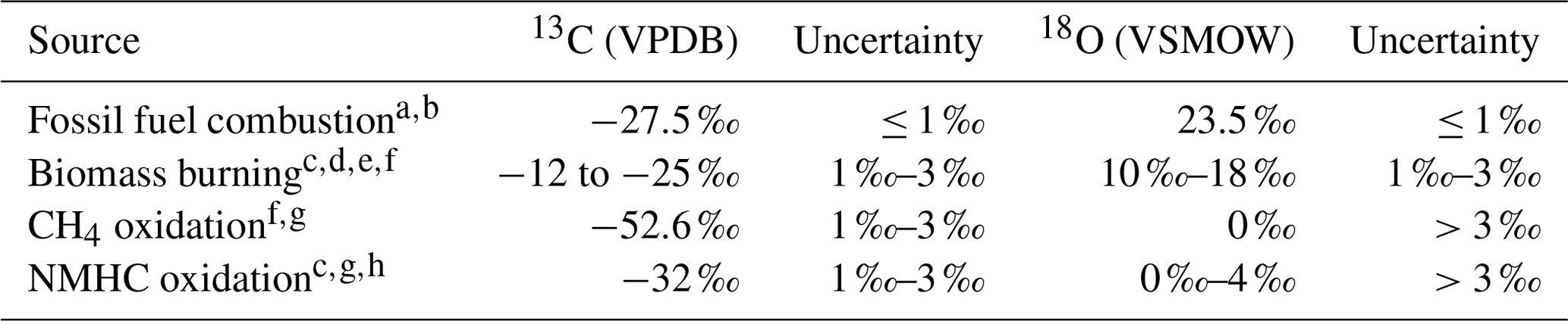
^a Stevens et al. (1972). ^b Brenninkmeijer (1993). ^c Stevens and Wagner (1989). ^d Bergamaschi et al. (1998). ^e Saurer et al. (2009). ^f Manning et al. (1997). ^g Brenninkmeijer and Röckmann (1997). ^h Vimont et al. (2019). Table based on the most recent compilation of source signatures by Vimont et al. (2019).

The method usually employed to determine the source signature of an observed pollution is to assume that a measured air parcel is the result of mixing of background air and a polluting source, i.e. two endmember mixing. Then the following mass balance applies to the mole fractions x:

$$\begin{array}{}\text{(1)}& x_{\mathrm{ap}}=f_{\mathrm{bg}}{x}_{\mathrm{bg}}+f_{\mathrm{src}}{x}_{\mathrm{src}},\end{array}$$

where ap denotes the air parcel, bg means background, and src means the pollution source. Here f_bg is the fraction of molecules of bg in ap, and f_src is the fraction of molecules of src; mass conservation requires $f_{\mathrm{bg}}+f_{\mathrm{src}}=\mathrm{1}$. A similar mass balance can be written for the stable isotopes:

$$\begin{array}{}\text{(2)}& x_{\mathrm{ap}}{\mathit{\delta }}^{\mathrm{13}}{\mathrm{C}}_{\mathrm{ap}}\approx f_{\mathrm{bg}}{x}_{\mathrm{bg}}{\mathit{\delta }}^{\mathrm{13}}{\mathrm{C}}_{\mathrm{bg}}+f_{\mathrm{src}}{x}_{\mathrm{src}}{\mathit{\delta }}^{\mathrm{13}}{\mathrm{C}}_{\mathrm{src}},\end{array}$$

since there is a small loss of tracer (Tans, 1980), hence the ≈ sign instead of =. Equations (1) and (2) can be solved to yield

$$\begin{array}{}\text{(3)}& {\mathit{\delta }}^{\mathrm{13}}{\mathrm{C}}_{\mathrm{ap}}=\left({\mathit{\delta }}^{\mathrm{13}}{\mathrm{C}}_{\mathrm{bg}}-{\mathit{\delta }}^{\mathrm{13}}{\mathrm{C}}_{\mathrm{src}}\right){\displaystyle \frac{f_{\mathrm{bg}}{x}_{\mathrm{bg}}}{x_{\mathrm{ap}}}}+{\mathit{\delta }}^{\mathrm{13}}{\mathrm{C}}_{\mathrm{src}},\end{array}$$

which results in a linear relation between δ¹³C_ap and $x_{\mathrm{ap}}^{-\mathrm{1}}$ if (δ¹³C_bg−δ¹³C_src)f_bgx_bg is assumed to be constant. This relation was first recognized by Keeling (1958) and is a special case of the more general Miller–Tans method (Miller and Tans, 2003). A relation for ¹⁸O, equivalent to Eq. (3), can be derived as well.

Two endmember mixing, as described above, can be safely applied to CO if it can be assumed that removal by OH is negligibly small. Recent applications of this methods can be found in e.g. Vimont et al. (2019), Vimont et al. (2017), and Gromov and Brenninkmeijer (2015). However, the age of the observed air parcel, 24–25 d (see Sect. 3.2), is too old to ignore the chemical reaction of CO+OH. Therefore the evolution of CO in the plume is modelled as follows:

$$\begin{array}{}\text{(4)}& {\displaystyle \frac{\mathrm{d}n\left(\mathrm{CO}\right)}{\mathrm{d}t}}=-k_{\mathrm{er}}\left(n\left(\mathrm{CO}\right)-n_{\mathrm{bg}}\left(\mathrm{CO}\right)\right)-k_{\mathrm{1}}n\left(\mathrm{OH}\right)n\left(\mathrm{CO}\right),\end{array}$$

where k_er is the entrainment rate in per second (s⁻¹). n(X) is the number density of species X, in per cubic centimetre (cm⁻³). The reaction rate of the reaction CO+OH, k₁, was taken from McCabe et al. (2001):

$$\begin{array}{}\text{(5)}& k_{\mathrm{1}}=\mathrm{1.57}\times {\mathrm{10}}^{-\mathrm{13}}+\mathrm{3.54}\times {\mathrm{10}}^{-\mathrm{33}}n,\end{array}$$

in cubic centimetres per second (cm³ s⁻¹), where n is the number density of air in per cubic centimetres (cm⁻³). The number density of OH is taken to be 2.7×10⁶ cm⁻³ between 0–4 km altitude, 1.6×10⁶ cm⁻³ between 4–8 km altitude, and 1.2×10⁶ cm⁻³ for altitudes >8 km (Mauzerall et al., 1998), although Mauzerall et al. (1998) specifies this value only for the range 8–12 km.

After separating the variables of Eq. (4), integrating, and solving for n(CO)(t) using the boundary condition that at $n\left(\mathrm{CO}\right)(t=\mathrm{0})=n_{\mathrm{0}}\left(\mathrm{CO}\right)$, this yields (see Appendix Sect. A for the derivation)

$$\begin{array}{}\text{(6)}& \begin{array}{rl}n\left(\mathrm{CO}\right)\left(t\right)& =\left(n_{\mathrm{0}}\left(\mathrm{CO}\right)+{\displaystyle \frac{k_{\mathrm{er}}{n}_{\mathrm{bg}}\left(\mathrm{CO}\right)}{-k_{\mathrm{er}}-k_{\mathrm{1}}n\left(\mathrm{OH}\right)}}\right)\\ & \exp \left(-\left(k_{\mathrm{er}}+k_{\mathrm{1}}n\left(\mathrm{OH}\right)\right)t\right)-{\displaystyle \frac{k_{\mathrm{er}}{n}_{\mathrm{bg}}\left(\mathrm{CO}\right)}{-k_{\mathrm{er}}-k_{\mathrm{1}}n\left(\mathrm{OH}\right)}}.\end{array}\end{array}$$

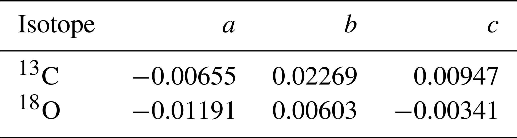
An equivalent equation to Eq. (6) can be written for ¹³CO and C¹⁸O. The reaction rates for these minor isotopologues can be determined from fractionation factors:

$$\begin{array}{}\text{(7)}& \mathit{\alpha }={\displaystyle \frac{k_{\mathrm{minor}}}{k_{\mathrm{major}}}}={\displaystyle \frac{\mathrm{1}}{a+bp+c{p}^{\mathrm{2}}}},\end{array}$$

where p is the atmospheric pressure in bar. The coefficients a, b, and c are fit to combined datasets from Röckmann et al. (1998), Stevens et al. (1980), and Smit et al. (1982), are obtained from Gromov (2013), and can be found in Table 2. k_minor and k_major are the reaction rates of the rare and abundant isotopologues respectively. We assume that k_major=k₁ as in Eq. (5).

Table 2 The coefficients a, b, and c for Eq. (7) for ¹³C and ¹⁸O.

Now k_er can be written as (see Sect. A for the derivation)

$$\begin{array}{}\text{(8)}& k_{\mathrm{er}}={\displaystyle \frac{-\ln \left(\mathrm{1}-f_{\mathrm{strat}}\right)}{t}}.\end{array}$$

If the age, t, of the air parcel is known, then k_er can be evaluated as a function of f_strat, which is the total fraction of stratospheric air entrained in the air parcel.

In principle f_strat is unknown, but it can be evaluated over the full range from 0 to 1 to provide a range of possible source signatures. Then this range can be compared to the signatures of possible sources (see Table 1). Furthermore, a best estimate can be made using f_strat found from Sect. 2.3.4.

Initial temperature and pressure are known from the observation made by LISA; temperature and pressure are assumed to be constant during transport. Then Eq. (6) can be used to obtain the CO, ¹³CO, and C¹⁸O number densities from which δ¹³C and δ¹⁸O can be determined throughout the simulation of the air parcel in the stratosphere.

2.3.4 Estimate of the tropospheric air fraction based on the in situ observations

The mass balances in Eqs. (1) and (2) can be extended to allow for more than two endmembers. Assuming mixing of stratospheric air, tropospheric air, and wildfire smoke, the mass balance for the mole fraction of the observed plume, here called the air parcel or ap, sampled by LISA can be written as

$$\begin{array}{}\text{(9)}& x_{\mathrm{ap}}=f_{\mathrm{w}}{x}_{\mathrm{w}}+f_{\mathrm{t}}{x}_{\mathrm{t}}+f_{\mathrm{s}}{x}_{\mathrm{s}},\end{array}$$

and for the stable isotopes, where the same approximation in Eq. (2), discussed in Sect. 2.3.3, is used, it can be written as

$$\begin{array}{}\text{(10)}& x_{\mathrm{ap}}{\mathit{\delta }}^{\mathrm{13}}{\mathrm{C}}_{\mathrm{ap}}=f_{\mathrm{w}}{x}_{\mathrm{w}}{\mathit{\delta }}^{\mathrm{13}}{\mathrm{C}}_{\mathrm{w}}+f_{\mathrm{t}}{x}_{\mathrm{t}}{\mathit{\delta }}^{\mathrm{13}}{\mathrm{C}}_{\mathrm{t}}+f_{\mathrm{s}}{x}_{\mathrm{s}}{\mathit{\delta }}^{\mathrm{13}}{\mathrm{C}}_{\mathrm{s}}\end{array}$$

and

$$\begin{array}{}\text{(11)}& x_{\mathrm{ap}}{\mathit{\delta }}^{\mathrm{18}}{\mathrm{O}}_{\mathrm{ap}}=f_{\mathrm{w}}{x}_{\mathrm{w}}{\mathit{\delta }}^{\mathrm{18}}{\mathrm{O}}_{\mathrm{w}}+f_{\mathrm{t}}{x}_{\mathrm{t}}{\mathit{\delta }}^{\mathrm{18}}{\mathrm{O}}_{\mathrm{t}}+f_{\mathrm{s}}{x}_{\mathrm{s}}{\mathit{\delta }}^{\mathrm{18}}{\mathrm{O}}_{\mathrm{s}}.\end{array}$$

Here f and x are defined in Sect. 2.3.3. Subscripts w, t, and s denote the wildfire smoke, tropospheric, and stratospheric endmembers respectively, whereas ap denotes air parcel. An endmember is defined here by its carbon and oxygen isotopic composition and by its mole fraction, and it is possible to distinguish the air parcel from others based on those parameters. Mass balance requires

$$\begin{array}{}\text{(12)}& f_{\mathrm{w}}+f_{\mathrm{t}}+f_{\mathrm{s}}=\mathrm{1}.\end{array}$$

This is an extension of two endmember mixing presented by Eqs. (1) and (2). Combining Eqs. (9), (12), (10), and (11) yields a system of four linear equations:

$$\begin{array}{ll}{\displaystyle }& {\displaystyle }\left[\begin{array}{ccc}\mathrm{1}& \mathrm{1}& \mathrm{1}\\ x_{\mathrm{w}}& x_{\mathrm{t}}& x_{\mathrm{s}}\\ x_{\mathrm{w}}{\mathit{\delta }}^{\mathrm{13}}{\mathrm{C}}_{\mathrm{w}}& x_{\mathrm{t}}{\mathit{\delta }}^{\mathrm{13}}{\mathrm{C}}_{\mathrm{t}}& x_{\mathrm{s}}{\mathit{\delta }}^{\mathrm{13}}{\mathrm{C}}_{\mathrm{s}}\\ x_{\mathrm{w}}{\mathit{\delta }}^{\mathrm{18}}{\mathrm{O}}_{\mathrm{w}}& x_{\mathrm{t}}{\mathit{\delta }}^{\mathrm{18}}{\mathrm{O}}_{\mathrm{t}}& x_{\mathrm{s}}{\mathit{\delta }}^{\mathrm{18}}{\mathrm{O}}_{\mathrm{s}}\end{array}\right]\left[\begin{array}{c}{f}_{\mathrm{w}}\\ f_{\mathrm{t}}\\ f_{\mathrm{s}}\end{array}\right]\\ \text{(13)}& {\displaystyle }& {\displaystyle }=\left[\begin{array}{c}\mathrm{1}\\ x_{\mathrm{ap}}\\ x_{\mathrm{ap}}{{\mathit{\delta }}^{\mathrm{13}}\mathrm{C}}_{\mathrm{ap}}\\ x_{\mathrm{ap}}{{\mathit{\delta }}^{\mathrm{18}}\mathrm{O}}_{\mathrm{ap}}\end{array}\right]+\left[\begin{array}{c}{M}_{\mathrm{r}}\\ x_{\mathrm{r}}\\ x_{\mathrm{r}}{{\mathit{\delta }}^{\mathrm{13}}\mathrm{C}}_{\mathrm{r}}\\ x_{\mathrm{r}}{{\mathit{\delta }}^{\mathrm{18}}\mathrm{O}}_{\mathrm{r}}\end{array}\right].\end{array}$$

The second term on the right-hand side, $[M_{\mathrm{r}},x_{\mathrm{r}},x_{\mathrm{r}}{\mathit{\delta }}^{\mathrm{13}}{\mathrm{C}}_{\mathrm{r}},x_{\mathrm{r}}{\mathit{\delta }}^{\mathrm{18}}{\mathrm{O}}_{\mathrm{r}}]$, is the residual vector that ensures equality of the over-constrained problem, with M_r denoting the normalized mass. Note that ideally this term is zero.

This set of equations is normalized to the observations and weighted so that all residuals are of equal importance, except for the mass balance. The mass balance was given extra weight, which conforms to the assumption that the observed air parcel is purely a mixture of tropospheric, stratospheric, and wildfire smoke.

Equation (13) was solved for f_w, f_t, and f_s by minimizing the residuals $[M_{\mathrm{r}},c_{\mathrm{r}},c_{\mathrm{r}}{\mathit{\delta }}^{\mathrm{13}}{\mathrm{C}}_{\mathrm{r}},c_{\mathrm{r}}{\mathit{\delta }}^{\mathrm{18}}{\mathrm{O}}_{\mathrm{r}}]$ using a non-negative least squares algorithm (Lawson and Hanson, 1995).

The values assumed for the endmember variables are presented in Table 3, rely on different sources, and will be discussed in detail below. All of the endmembers have a different uncertainty. In order to capture the effect of these uncertainties, a Monte Carlo simulation was performed, rather than a single calculation, to estimate f_w, f_t, and f_s. The endmember values are randomly drawn from the respective distributions assumed, also presented in Table 3.

The stratospheric endmember definition and the plume observation are based on the balloon-borne observations by LISA, outside and inside the plume, respectively (see Table 4). The plume mole fractions are assigned an uncertainty equal to the measurement uncertainty of LISA. The uncertainty of the stratospheric endmember is also a good measure of the variability surrounding the plume based on AirCore measurements between 12 and 14.5 km of 6 and 7 September. The uncertainty of the isotopic composition in the Monte Carlo simulation is set equal to twice the measurement uncertainty (see Sect. 2.2.3) because the stratospheric variability of the stable isotopic composition of CO is unknown. Secondly, there may have been a small drift in the isotopic composition.

In an additional Monte Carlo experiment, the plume observation is corrected for removal by OH, using Eq. (6) with k_er=0. t is equal to the 25 d of transport. This definition of the plume observation appears in Table 3 as “ap OH-corrected”. A number density OH of 1.2×10⁶ cm⁻³ is used in the calculation.

Table 3 Endmember variables and air parcel values and uncertainties as used in the Monte Carlo simulation. Mole fractions are given in part per billion (ppb) and δ values in per mille (‰). Here ap means air parcel and is based on the in situ observation made by LISA (see Table 4). The uncertainties for the mole fractions is set equal to the uncertainty of the LISA observations as discussed in Sect. 2.2.1. The uncertainty of the isotopic composition of the stratosphere, ap, and ap OH-corrected are set equal to twice the measurement uncertainty; see text for a discussion. In the ap OH-corrected, ap is corrected for removal by OH using Eq. (6) with k_er=0. A number density OH of 1.2×10⁶ cm⁻³ is used. The stratospheric endmember definition is based on the in situ observation of stratospheric background presented in Table 4. The tropospheric and wildfire smoke endmember definitions are based on observations from earlier work (see text). The large range for the plume mole fraction does not significantly affect the results of the Monte Carlo simulation.

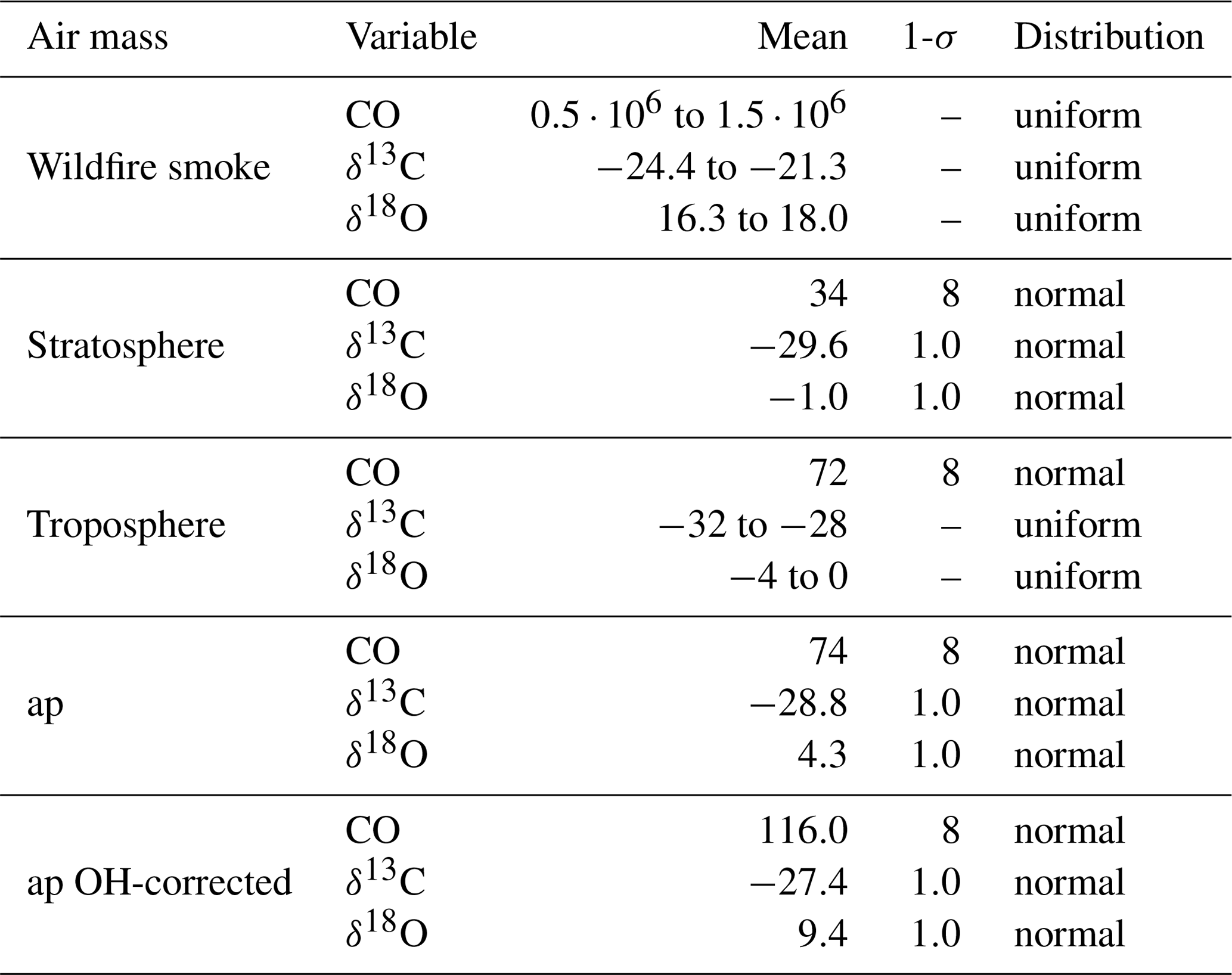
The wildfire smoke and tropospheric endmember rely on measurements from earlier publications, which introduces a large uncertainty on endmember definitions. First of all, the isotopic composition and mole fraction of tropospheric CO exhibits temporal, both seasonal and annual, and latitudinal gradients (Bergamaschi et al., 2001; Mak et al., 2003), which complicates the characterization of the tropospheric endmember. The smoke source region lies between 65 and 75^∘ N (see Sect. 3.2), with south-westerly surface winds coming from the Pacific Ocean (Peterson et al., 2018). Tropospheric CO mole fractions used are based on measurements of CO from Sand Island, Midway (Petron et al., 2019), and reported to be typically 72±8 ppb in the 6 weeks preceding the event. The range of isotopic-composition values considered is therefore obtained from measurements made at Izana (28^∘ N and 16^∘ W, which is representative for CO in air that travels over the ocean at mid-latitudes. δ¹³C ranges between −32 ‰ and −28 ‰ and δ¹⁸O ranges between −4 ‰ and 0 ‰ (Bergamaschi et al., 2001; Mak et al., 2003). The mole fractions obtained here from Midway island are consistent with those co-reported with the δ¹³C and δ¹⁸O ranges by Bergamaschi et al. (2001) and Mak et al. (2003).

In addition, the wildfire smoke signature (see Table 1) is subjected to a large variability due to the type of burned plants (categorized as C₃ or C₄, with a difference in photosynthesis), the burning temperature, and possibly the groundwater isotopic composition (Kato et al., 1999). Since the wildfire originated in Canada, the fuel consisted mainly of C₃ plants, which are typically more depleted in δ¹³C. Furthermore, the fire was energetic enough to trigger a pyro-Cb event, which makes it reasonable to assume that it was in an efficient burning regime, which typically leads to higher δ¹⁸O. Therefore, the range of isotopic composition of CO of the wildfire smoke assumed here is according to atmospheric measurements around forest fires (Brenninkmeijer et al., 1999; see Table 3). This is thus a subset from the range of signatures displayed in Table 1, which provide a more general summary.

The mole fraction of wildfire smoke is also an unknown, but it is clear that it is far larger than both the stratospheric and tropospheric background mole fraction; thus a large mole fraction ensures, by virtue of Eq. (12), f_w≪f_s and f_w≪f_t.

Since the mole fraction and isotopic composition of the smoke plume and the tropospheric endmembers are ill-defined, partially due to natural variability, the Monte Carlo results are filtered. Solutions to Eq. (13) are only allowed if the residuals are smaller than the measurement 1σ uncertainty attributed to our stratospheric observations, e.g. 8 ppb for the mole fractions and 0.5 ‰ for the δ values. A solution is thus only allowed when it is consistent with the observations and the reported isotopic-composition range published in literature. Furthermore, the solution requires all fractions to be larger than 0, where four significant figures were considered, to avoid a large amount of unrealistic solutions.

3 Results

3.1 Observation of a stratospheric CO enhancement

The CO measurements of both the LISA sampler and the AirCore are presented in Fig. 1a. A clear carbon monoxide enhancement was observed between 13 and 14 km altitude on 4 and 5 September 2017. The plume, extending over roughly 1 km in altitude, was well above the tropopause, which can be seen from the CO gradient below 13 km. The tropopause height was determined based on the lapse rate from the radiosonde temperature measurements to be 12 km on both flights, confirming that the observed plume is above the tropopause. The potential temperature was θ≈350 K at 13 km and θ≈380 K at 14 km, which classifies this part of the stratosphere as the extratropical lowermost stratosphere (Holton et al., 1995). The observed CO₂ mole fraction Fig. 1b showed a slight increase in the same layer, which allowed for determination of the enhancement ratio, ΔCO:ΔCO₂ (see Sect. 3.3).

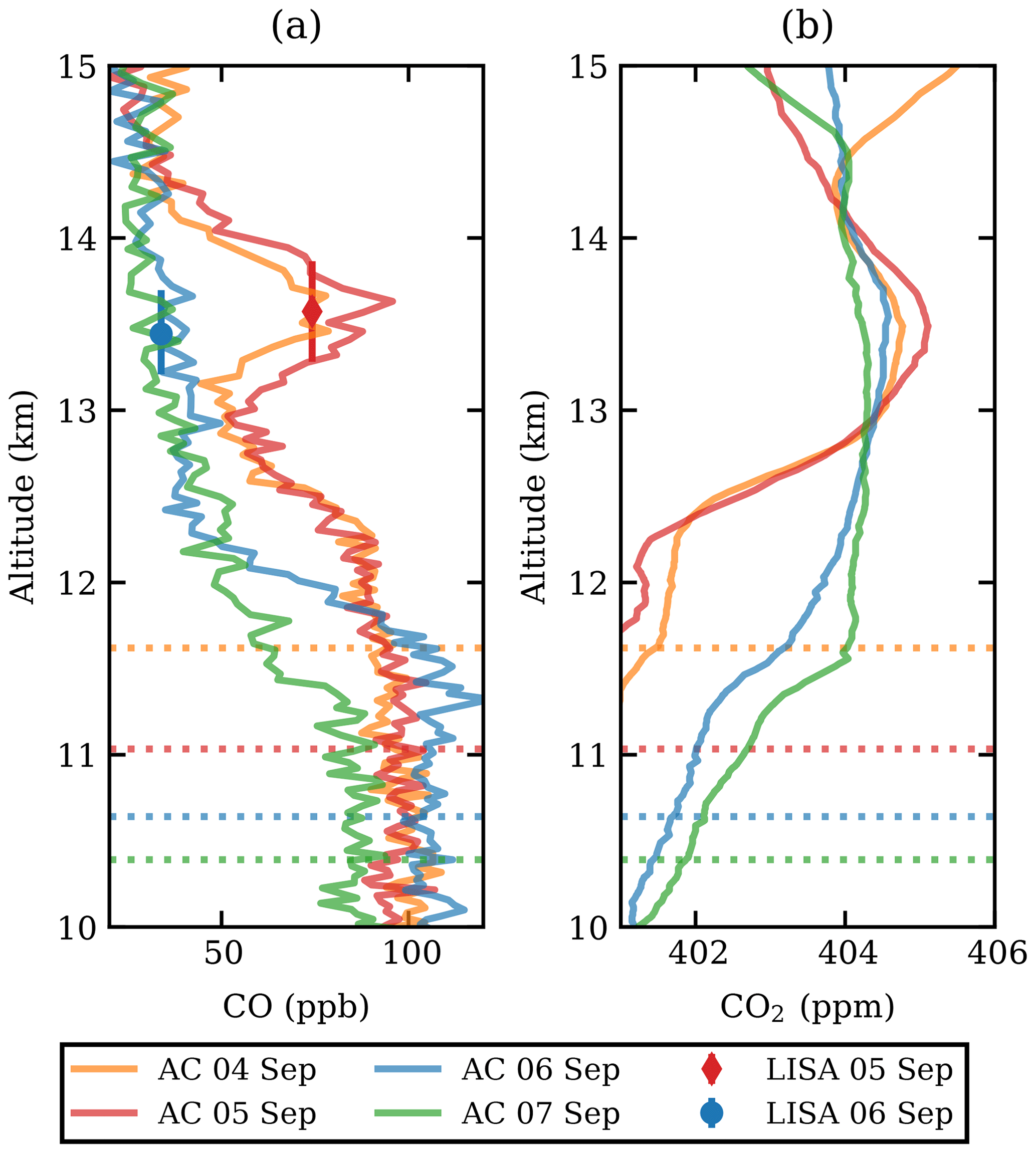
Figure 1 The CO (a) and CO₂ (b) profiles from AirCore (lines, abbreviated as AC in the legend) and the LISA sampler (markers). The profiles are shown between 12 and 15 km altitude and are coloured by date. The LISA sampler vertical error bars represent the total vertical coverage of the sample, with the mean altitude as shown. For mole fraction measurement uncertainties, the reader is referred back to Sect. 2.2.1. The tropopause is indicated as a dashed line, matching the colour of the respective AirCore flight.

3.2 Origin and age of the plume based on back-trajectory analysis

A first set of six back trajectories was initialized from the altitude of the observed CO-peak maximum (p=155 hPa, 13.6 km) and the altitudes where the CO enhancement was half of the maximum (166 and 148 hPa, 13.3–13.8 km; see Fig. 1) starting on 4 and 5 September. After that, matches with CALIOP night-time observations were determined as follows. For each orbit time, the minimum distance of the trajectory and the orbit location was calculated. Wherever the distance was smaller than 250 km, the observed backscatter ratio was investigated for nearby atypical aerosol enhancements. In this way the smoke could be traced back to the injection date and region.

Figure 2a shows the CALIOP backscatter ratio at 532 nm (R₅₃₂) as well as the location of the back-trajectory result on 3 September, with a match distance of 47 km for the lower starting altitude of the trajectories starting on 4 September. The match distances of the trajectories from the centre and upper altitude are above 250 km (282 and 434 km) and are not shown here. To track the aerosol cloud, new back trajectories were initialized starting from 3 September exactly where aerosol cloud is observed in the CALIOP data (Fig. 2b, white crosses). Other matches between back-trajectory location and CALIOP overpass were always at a layer of aerosol enhancement and no new back trajectories were initialized. These match results are not shown.

Figure 2 Altitude–longitude plot with CALIOP backscatter ratio and back-trajectory results. The red line indicates the thermal tropopause from CALIOP. (a) A match on 3 September between CALIOP and the lower CLaMS back trajectory starting on 4 September, indicated by the white cross. The distance between the back-trajectory result and the plotted white cross is 47 km. (b) Newly initialized back trajectories on 3 September (white crosses). (c) The matches on 20 August, between CALIOP backscatter and the results from the back trajectories initialized on 3 September, where the distance between back trajectory result and CALIOP overpass is smaller than 250 km. Note the altitude discrepancy showing that the vertical displacement is not precisely reproduced in the model. (d) Newly initialized back trajectories on 20 August. (e) Match location on 13 August with a vertical distance of 3 km to the aerosol plume. (f) Match location on 12 August with no clear correspondence between the trajectory and the enhanced backscatter from CALIOP. The time of the location match is well before the fires, 21:00 UTC (Peterson et al., 2018).

Again matches with CALIOP orbits were calculated. Figure 2c and d are similar to Fig. 2a and b but for 20 August, where a difference in altitude is observed. This altitude mismatch might be due to the additional vertical motion related to additional radiative heating of the smoke plume, which is absent in the CLaMS model. Similarly to 3 September, in a third step, back trajectories were calculated from this observed aerosol cloud. On 14 August, the back-tracked air parcels are within the range of the aerosol cloud that was observed by the Ozone Mapping Profiler Suite (OMPS), as shown by Peterson et al. (2018). Figure 3a shows the computed trajectories and the locations where re-initialization was performed. The result of the back-trajectory analysis is shown to match the location of the aerosol enhancement observed by OMPS and CALIOP in Fig. 3b.

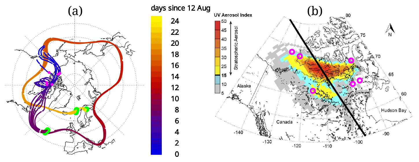
Figure 3 (a) Shows the computed trajectories. The three green areas show the location of the initialization and the two locations where the back trajectories are corrected, mainly in altitude, using a CALIOP match. The latter two correspond to the panels (a) and (b) as well as (c) and (d) in Fig. 2. The colour gradient shows days elapsed since 12 August. The pink circles in the figure on the left are showing the same location as in the figure on the right, (b). On the right, (b) a reprint of the figure from Peterson et al. (2018, Fig. 3) showing the ultraviolet aerosol index from the Ozone Mapping Profile Suite (OMPS) on 14 August with the CALIPSO satellite track in black. Here the results of the back trajectory on 14 August are added to the figure (pink circles), coinciding with the stratospheric smoke plume. The original figure was published under a Creative Commons Attribution 4.0 International License, http://creativecommons.org/licenses/by/4.0/, last access: 20 November 2020.

Figure 2f shows the location on 12 August, before the injection. This cloud is located over British Columbia and was caused by the pyro-convection as concluded by Peterson et al. (2018). Further back in time, the CALIOP backscatter data do not show any aerosol enhancement where a location match between CALIOP and the back trajectory was found. Therefore, the origin of the observed plume could be confirmed by this piecewise trajectory analysis that accounts for the vertical transport due to heating caused by the fire. Furthermore, the age of the plume at the time of observation was 24–25 d.

3.3 Enhancement ratios of CO/CO₂ of the plume

Figure 4 shows a scatter plot of the observed CO and CO₂ mole fractions in the plume, both measured CO and CO₂ data and CO corrected for removal by OH (see below). The enhancement ratio on 4 September, 40±2 ppb ppm⁻¹, is higher than that on 5 September, 34±1 ppb ppm⁻¹. The mole fraction enhancement ratio, 34–40 ppb ppm⁻¹, falls in the range of fresh to aged biomass burning plumes, as defined by Mauzerall et al. (1998). The regression coefficients are high (r²>0.8).

The chemical lifetime of CO against removal by OH is about 50 d in the stratosphere (e.g. Mauzerall et al., 1998). Since the age of the plume after the injection date of 12 August 2017 (Peterson et al., 2018) was 24 and 25 d for the observation on 4 September and 5 September 2017, respectively, the mole fraction of CO in the plume was thus significantly affected by chemical loss due to the reaction of CO with OH. Therefore, the observed CO mole fractions are corrected by assuming a continuous removal by OH, an approach similar to the one used by Andreae et al. (2001), using the parameters presented by Mauzerall et al. (1998).

Peterson et al. (2018) estimated the time of updraught in the troposphere to be 5 h; thus the plume was transported dominantly in the stratosphere. The dilution of the plume due to mixing with ambient air is ignored in the calculation. The OH-corrected enhancement ratios are plotted in Fig. 4. The corrected enhancement ratios are 53±2 and 62±3 ppb ppm⁻¹ for the 2 d respectively. Using the uncorrected enhancement ratios, the loss of CO was estimated about 35 %–37 %.

Using the data obtained from the 6 September flight as background, the following enhancement ratios are calculated: 45±1 ppb ppm⁻¹, uncorrected for OH, and 177±2 ppb ppm⁻¹, using a correction for removal by OH for 4 September (number of data points N=5); 91±29 ppb ppm⁻¹, uncorrected for OH, and 201±56 ppb ppm⁻¹, using a correction for removal by OH for 5 September (N=50). These are higher than those obtained from the linear fit, which is likely caused by relatively large uncertainties of the small ΔCO₂ values.

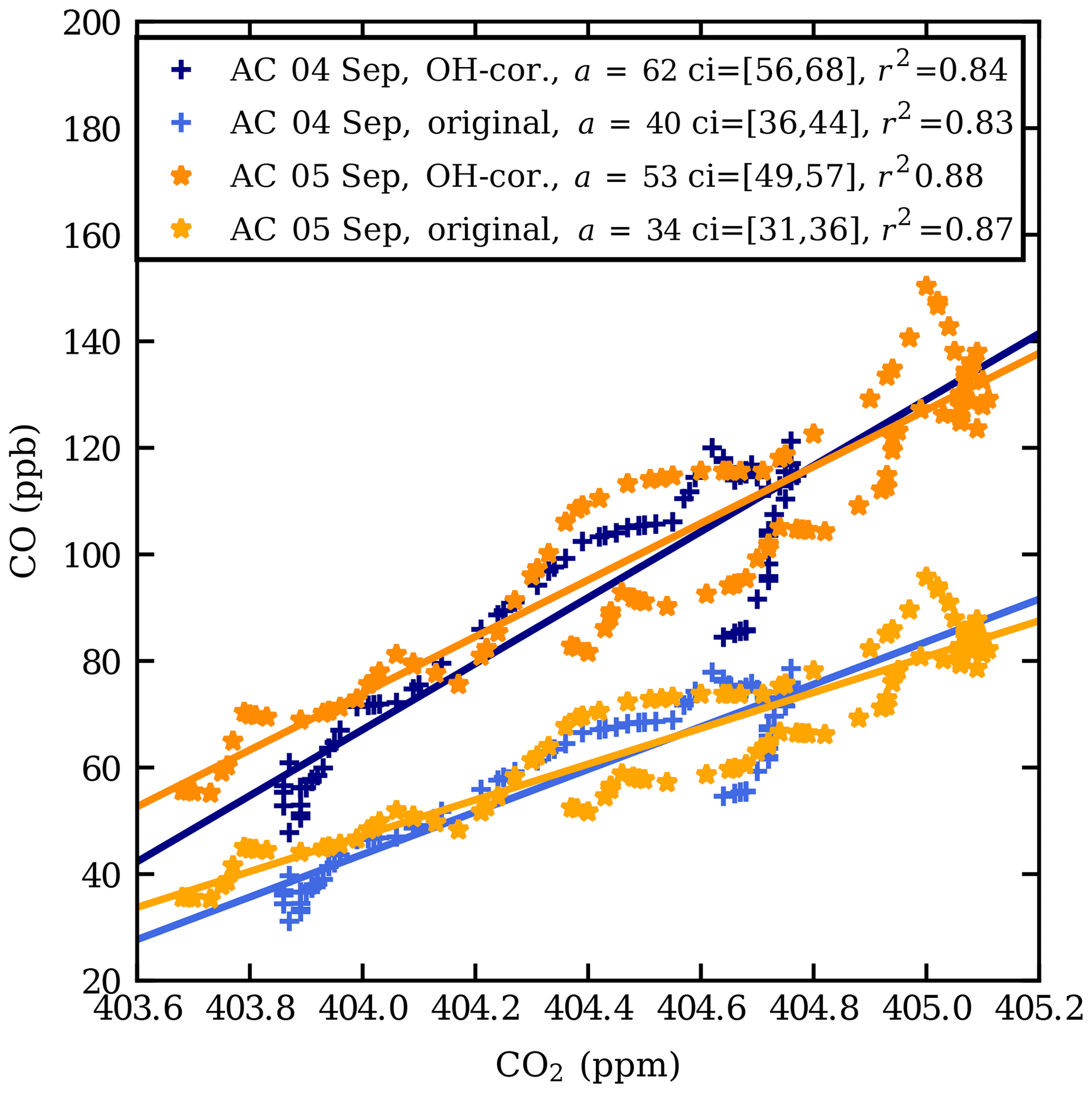
Figure 4 CO vs. CO₂ scatter plot at the observed CO enhancement in the AirCore (AC) profiles from 4 and 5 September 2017. The data shown are between the pressure levels 167 and 140 hPa (13.2–14.3 km) on 4 September and between 175 and 140 hPa (12.9–14.4 km) on 5 September. The lighter shades of orange and blue show the original values and the darker shades the CO values corrected for oxidation by OH. a is the fitted slope and ci is the 95 % confidence interval of the fitted slope.

3.4 CO stable isotope composition

The LISA sampler CO mole fractions and stable isotope analysis results are presented in Table 4. Two types of samples can be distinguished: a plume sample and a background sample. It can been seen from Table 4 that the difference in their mole fraction and δ¹⁸O is pronounced, whereas the δ¹³C values are similar.

Table 4 LISA observations of CO, mole fractions and the carbon and oxygen isotopic composition of CO, of the plume, P, and background, B. Here δ¹³C(CO) is reported in per mille (‰) vs. VPDB and δ¹⁸O(CO) in per mille (‰) vs. VSMOW.

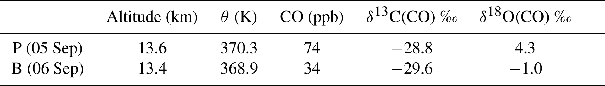
The sample taken on 6 September can be considered as a background value for two reasons. First of all, the mole fraction measurements from both LISA and AirCore agree with those of normal NH CO stratospheric mole fractions (Hoor et al., 2005). Secondly, the δ¹³CO agrees to within ±1 ‰ compared to the measurements performed in the Southern Hemisphere lowermost stratosphere (Brenninkmeijer et al., 1995). Note that tropospheric CO and its isotopic composition exhibit a latitudinal gradient and a seasonal cycle, related to the OH sink. It is not exactly known whether and to what extent these gradients exist in the stratosphere, and thus the agreement may be incidental.

The δ¹⁸CO in the Southern Hemisphere SH is about 7.2 ‰ more depleted compared to the background value found from the observation presented here. Brenninkmeijer et al. (1995) attributed the relatively low values of ¹⁸O to two determining factors: the unknown but probably low source signature for oxygen of methane-derived CO and the inverse kinetic isotope effect in the reaction with OH that depletes CO in ¹⁸O. Nonetheless, lower δ¹⁸O values are typically a sign of absence of any nearby sources other than oxidation of atmospheric methane (Brenninkmeijer et al., 1999).

The LISA CO mole fraction measured on 5 September compares best to the AirCore measurement of the day before and is in the middle of the plume (see Fig. 1). We thus assume that the isotopic composition of that particular sample is representative for that in the plume. A comparison of the different δ¹⁸O values, in Table 4, clearly shows that the CO plume is different than the background. Although the observed difference in δ¹³C between the plume and the background sample is significant (0.8 ‰), it could also be the result of natural variability. Furthermore, many sources carry a comparable δ¹³C signature (see Table 1).

3.5 Source signature based on isotopic composition of CO

Determining the source signature of the enhancement is not straightforward because of two reasons. First, the plume sample was affected by mixing in the troposphere during updraught and by mixing in the stratosphere. Secondly, the plume CO has been altered significantly by reaction with OH over the 25 d transport time. Thus, as explained in Sect. 2.3.3 the simple Keeling approach does not apply here.

Both the tropospheric background CO in NH summer (Bergamaschi et al., 2001; Mak et al., 2003) and stratospheric background CO, see Table 4, are more depleted in ¹⁸O than the CO in the plume. Thus, mixing would decrease the δ¹⁸O of the plume. Since tropospheric and stratospheric δ¹³C(CO) are alike (see Table 3), δ¹³C is not obviously affected by mixing.

In addition to mixing in the stratosphere, the reaction with OH is associated with an inverse isotope effect at stratospheric pressure for both ¹³C and ¹⁸O, depleting the remaining CO in both ¹³C and ¹⁸O (Röckmann et al., 1998). Thus, both removal by OH and mixing make the plume CO more depleted in ¹⁸O, whereas the observed δ¹⁸O value in the plume is higher than in the background. The δ¹³C value is mainly affected by OH. The plume isotopic composition was thus originally more enriched in both ¹⁸O and ¹³C.

Equation (4) is used to estimate the CO mole fraction and oxygen and carbon isotopic composition of the plume 25 d before the observations as a function of the unknown stratospheric fraction of air mixed into the sample, f_strat. It is assumed that pressure and temperature remained constant during transport. The number density of OH assumed for the stratosphere is $n\left(\mathrm{OH}\right)=\mathrm{1.2}\times {\mathrm{10}}^{\mathrm{6}}$ cm⁻³. The model results show that the isotopic composition of the plume would have been $-\mathrm{27.5}\mathrm{‰}\le \mathit{\delta }{}^{\mathrm{13}}\mathrm{C}\le -\mathrm{26.6}\mathrm{‰}$ and $\mathrm{10}\mathrm{‰}\le \mathit{\delta }{}^{\mathrm{18}}\mathrm{O}\le \mathrm{14}\mathrm{‰}$ after injection into the stratosphere (see Fig. 5). This range corresponds to the modelled results for $n\left(\mathrm{OH}\right)=\mathrm{1.2}\times {\mathrm{10}}^{\mathrm{6}}$ cm⁻³. Figure 5 also shows results of the same calculations assuming OH number densities twice as high and no oxidation by OH.

Using the OH-corrected estimate of f_strat=0.55 from the Monte Carlo simulation in Sect. 3.6, the plume δ¹³C and δ¹⁸O, directly after injection in the stratosphere, are estimated to be −27.0 ‰ and 11.4 ‰ respectively. Hence, the fractionation that occurred during transport depleted ¹³C by 1.8 ‰ and 7.1 ‰ ¹⁸O.

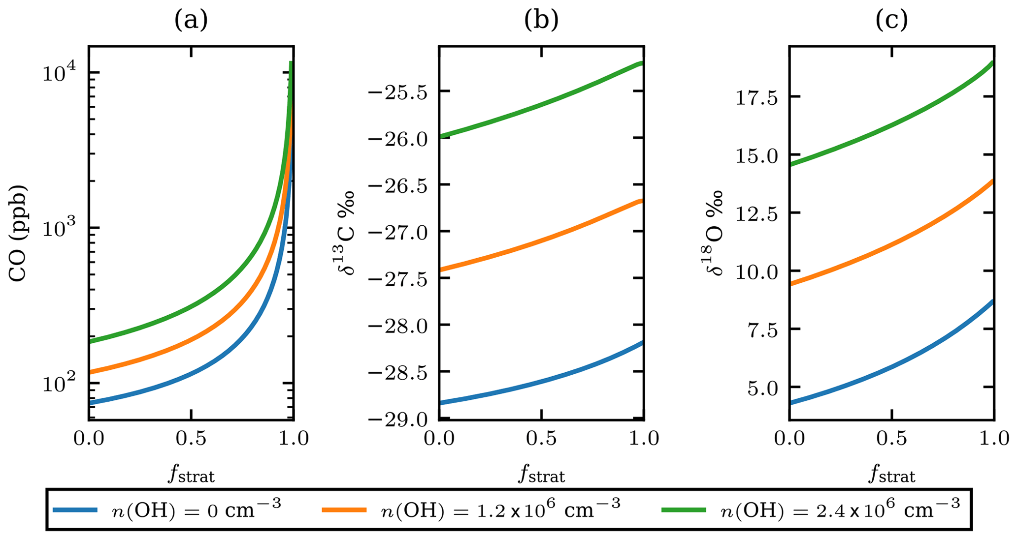
Figure 5 The estimated CO mole fractions on a logarithmic scale (a), the carbon (b), and oxygen (c) isotopic composition of the plume CO for different OH number densities versus f_strat just after injection into the stratosphere. OH number densities are shown in the legend; the value of 1.2×10⁶ can be considered representative of the stratosphere. The value of 2.4×10⁶ is arbitrarily added as twice the stratospheric value and serves as an upper estimate.

Note that when the number density of OH is 0 cm⁻³ Eq. (4) describes simple endmember mixing with rate k_er. If the Keeling method is applied, a source signature of ${\mathit{\delta }}^{\mathrm{13}}{\mathrm{C}}_{\mathrm{src}}=-\mathrm{28.1}$ and δ¹⁸O_src=8.7 is obtained, providing a lower limit of the source signature. Upper limits for the source signature are derived assuming a very large amount of stratospheric mixing and high OH number density; the source signature has $\mathit{\delta }{}^{\mathrm{13}}\mathrm{C}<-\mathrm{22}$ ‰ and δ¹⁸O<21 ‰. Based on the analysis in the preceding paragraphs, the source signature of the plume origin has $-\mathrm{27.5}\mathrm{‰}\le \mathit{\delta }{}^{\mathrm{13}}\mathrm{C}\le -\mathrm{22}\mathrm{‰}$ and $\mathrm{10}\mathrm{‰}\le \mathit{\delta }{}^{\mathrm{18}}\mathrm{O}\le \mathrm{21}\mathrm{‰}$.

The analysis above shows that the plume was initially more enriched in both¹³C and ¹⁸O than at the time of observation. Comparing the derived signature to the source signatures in Table 1, it is clear that the source signature is similar to that of CO produced in wildfires. In fact, qualitatively, the plume was more enriched, then computed in Fig. 5, if we would correct for the tropospheric air mixed into the air parcel. Then the values for the troposphere presented in Table 3 have to be assumed, and the source signature comes close to the expected range of isotopic compositions for the wildfire presented in this study (Table 3).

Fossil fuel combustion sources, the only other source that produces CO containing higher δ¹⁸O, can be excluded for two reasons. First, the source signature of high-temperature combustion, ∼23.5 ‰, is outside the calculated range of the source signature. Secondly, the enhancement ratio of ΔCO:ΔCO₂ is too high for modern day fossil fuel combustion (see e.g. Popa et al., 2014).

On the basis of the observed δ¹³C signature, CH₄ oxidation can be excluded as a source, as methane-derived δ¹³C is usually far more depleted (Brenninkmeijer et al., 1999). Finally, oxidation of non-methane hydrocarbons (NMHCs) can be excluded as a significant source. The total amount of NMHCs in the stratosphere is on the order of several parts per trillion (ppt Scheeren et al., 2003). Furthermore, estimates of the NMHCs source signature suggest that the oxygen signature is in the range 0 ‰–3.6 ‰ (Brenninkmeijer and Röckmann, 1997; Vimont et al., 2019). The NMHCs produced in the fire have a mean enhancement ratio to CO of the order of parts per trillion per part per million (ppt ppm⁻¹; Mauzerall et al., 1998) and thus would result in a very small in situ source of CO that would have a very small effect on the isotopic composition.

3.6 Estimate of the tropospheric air fraction based on the in situ observations

The fractions of tropospheric, f_p, and stratospheric air, f_s, in the plume were determined using Eq. (13). The results of two Monte Carlo simulations are shown in Fig. 6: one simulation with CO observation corrected for OH and one without the correction. The mean of each distribution suggests that the tropospheric air fraction is 48±21 % and the stratospheric fraction is 52±21 %. After the correction for oxidation, this shifts the tropospheric contribution to 45±21 % and the stratospheric contribution to 55±21 %. Thus, ignoring the oxidation results in a small bias in the estimated stratospheric and tropospheric contribution to the plume.

Figure 6 Probability density of the air fraction by volume, as a result of a Monte Carlo simulation. The data are binned into 1 % bins. Results with and without a correction for OH are shown.

4 Discussion

4.1 Enhancement ratios and plume age

Initially, the plume was observed from a clear CO mole fraction increase in the stratosphere, present in two AirCore profiles. The CO plume mole fraction measurements, up to 90 ppb, are lower compared to other plumes measured in the stratosphere, notably by Waibel et al. (1999) (300 ppb), Jost et al. (2004) (200 ppb), and by Cammas et al. (2009) (250 ppb). First, the plume reported is older than other observations. The estimated plume age was 25 d, where the other observations were sampled after 7 to 14 d. Hence, the plume observed here was affected more by mixing and photochemistry in the stratosphere. Secondly, it is unlikely that the accidental encounter sampled the centre of the plume where CO mole fractions are highest. Finally, it should be pointed out that the plume was encountered during AirCore vertical profiling, which has limited the vertical resolution that could smooth out the maximum values.

In addition to the anomalous CO mole fraction, enhancement ratios of CO vs. CO₂ obtained from the regression analyses, based on concurrent AirCore CO₂ and CO measurements, agree with the ratios obtained in previous studies on biomass burning emissions. The observed ratios of 34–40 ppb ppm⁻¹ in this study are lower than the measured enhancement ratios of 50 ppb ppm⁻¹ by Jost et al. (2004) and 48–73 ppb ppm⁻¹ by Andreae et al. (2001). The plumes reported by both Jost et al. (2004) and this study originated from forest fires in North America (40–55^∘ N) and were observed at a similar altitude of approximately 1.5 km above local tropopause. It is a reasonable assumption that the initial enhancement ratios and the mixing of the plumes with lower stratospheric backgrounds are similar. However, the plume age of roughly 25 d in this study is significantly older than that of 10–14 d observed by Jost et al. (2004). Therefore, the ageing of the plume coupled with the OH-related destruction of CO likely explains the difference in the observed ratios. Similarly, the age of 9–10 d of the plumes observed by Andreae et al. (2001) is also significantly younger than the plume age found in this study. Indeed, the OH-corrected enhancement ratios of 53–62 ppb ppm⁻¹ in this study come closer to the similar OH-corrected enhancement ratios of 64–98 ppb ppm⁻¹ in Andreae et al. (2001), and the remaining difference may be caused by the different type of fuels of biomass burning: forest in this study and savannah/forest in Andreae et al. (2001).

The enhancement ratios computed directly are much higher than the results discussed above. First, it is difficult to assume what background should be used. The stratospheric background mole fractions, especially the CO₂, vary with altitude and in time, e.g. comparing the AirCore profiles from 6 and 7 September, which questions the assumption of a constant background. It is thus difficult to state with certainty that data from 6 September are representative for the background. However, as the plume and air directly adjacent to it move together, it can be assumed that the air surrounding the plume has constant mole fractions. The best estimates of the mole fractions are those measured above and below the plume, obtained from the vertical profile. Hence, the most reliable estimate of the enhancement ratio is obtained from the regression analysis discussed above. On a final note, the very small standard deviation of 1–2 ppb obtained for 4 September is largely due to the small amount of data, N=5, and the large averaging window of 25 data points.

4.2 Isotopic composition of plume CO

The stable isotope source signatures of CO supports wildfire smoke as the source. The δ¹⁸O source signatures for Siberian boreal forest fires (14.8 ‰ and 9.0 ‰, reported by (Bergamaschi et al., 1998) and (Tarasova et al., 2007) respectively) compare well with the observation made in this work after estimating the fractionation that occurs during oxidation (see Sect. 3.5).

Brenninkmeijer and Röckmann (1997) reported a source signature of 4.5 ‰ for wildfire smoke, based on Southern Hemisphere observations. As argued by Brenninkmeijer and Röckmann (1997) the samples must have been affected by the strong fractionation accompanying the reaction of CO with OH along the mixing, something that was not accounted for in their method used to derive the source signature. The lifetime of CO against removal by OH in the stratosphere is considerably longer than in the troposphere, and hence the wildfire sample presented here was likely less affected by fractionation than their measurement.

It is shown that CO stable isotope measurements can help pollution events in the stratosphere to be identified. It must be noted that this study took advantage of the fact that, on the days following the pollution event, clean background air was sampled. Thus, a direct comparison of background air and polluted air was possible. Without the measurement of background air, source attribution would have been difficult from stable isotope measurements, as little is known about the CO isotopic composition. Fundamental knowledge of CO isotopic composition, and its temporal and latitudinal variation in the stratosphere is vital for the detection of future pollution events based on CO measurements.

In addition to a poorly understood isotope budget of the stratosphere, the case made in this study would have been stronger if the oxygen signature of both methane and NMHCs were known more precisely. Our fundamental knowledge of the CO isotopic composition in the stratosphere would also benefit from those measurements, as methane is the main source of CO in the stratosphere.

4.3 Assessment of tropospheric and stratospheric air mass contributions

Finally, the air mass fractions of the troposphere and stratosphere were derived using the tracer observations. The results suggest that the 2017 pyro-Cb plume observed above Sodankylä consists of approximately 45±21 % tropospheric air polluted with wildfire smoke. This is comparable to the model simulations from Trentmann et al. (2006) on the Chisholm fire in 2001, an event similar to the 2017 British Columbia fires. Cammas et al. (2009) modelled their observations of wildfire smoke from several fires in Canada and Alaska, and they estimated the amount of polluted boundary layer air above the tropopause to be 15 %–20 %.

5 Conclusions

A wildfire smoke plume in the lower stratosphere was investigated using in situ observations of CO and CO₂ from AirCore and stratospheric δ¹³C and δ¹⁸O in CO from LISA. The plume was identified by enhanced CO mole fractions at approximately 13.6 km altitude, present on 2 consecutive days, and extending over 1 km in altitude. The plume's enhancement ratio of CO to CO₂ mole fractions was in the range 34–40 ppb ppm⁻¹. The stable isotopic composition of carbon and oxygen in CO support wildfire smoke as the source for the enhanced CO mole fractions observed in both AirCore and LISA samples. Using the CLaMS back-trajectory module and CALIOP backscatter data, the source region is determined to be British Columbia, Canada. The smoke was injected on 12 August 2017, 24–25 d before the observations were made. The age of the plume aided in the estimation of the amount of oxidation, a 35 %–37 % loss of CO, and the accompanying isotopic fractionation, 1.8 ‰ for δ¹³C and 7.1 ‰ δ¹⁸O. Using this information, the enhancement ratios corrected for oxidation ranged from 53 to 62 ppb ppm⁻¹. The plume isotopic composition of oxygen and carbon in CO was estimated to be −27.0 ‰ and 11.4 ‰. From the LISA observations, it was possible to determine the fractions of tropospheric, 45±21 %, and stratospheric air, 55±21 %, in the plume using a three-endmember mixing model.

Appendix A: Derivation of Eqs. (6) and (8)

A constant entrainment rate is assumed; i.e. so that

$$\begin{array}{}\text{(A1)}& {\displaystyle \frac{\mathrm{d}V}{\mathrm{d}t}}=kV.\end{array}$$

This can be solved to yield

$$\begin{array}{}\text{(A2)}& V\left(t\right)=V_{\mathrm{0}}\exp \left(kt\right),\end{array}$$

with V₀ the initial volume of the air parcel containing the contamination. Thus $V_{\mathrm{0}}/V_t=f_{\mathrm{plume}}$ and

$$\begin{array}{}\text{(A3)}& V\left(t\right)=f_{\mathrm{plume}}{V}_{\mathrm{plume}}+f_{\mathrm{strat}}{V}_{\mathrm{strat}},\end{array}$$

with $f_{\mathrm{plume}}+f_{\mathrm{strat}}=\mathrm{1}$. Then Eq. (A2) can be written as follows:

$$\begin{array}{}\text{(A4)}& \mathrm{1}-f_{\mathrm{strat}}=\exp \left(-kt\right).\end{array}$$

This can be rearranged to give the end result, k in terms of f_strat:

$$\begin{array}{}\text{(A5)}& k={\displaystyle \frac{-\ln \left(\mathrm{1}-f_{\mathrm{strat}}\right)}{t}}.\end{array}$$

Starting from Eq. (6),

$$\begin{array}{}\text{(A6)}& {\displaystyle \frac{\mathrm{d}n\left(\mathrm{CO}\right)}{\mathrm{d}t}}=-k_{\mathrm{er}}\left(n\left(\mathrm{CO}\right)-n_{\mathrm{bg}}\left(\mathrm{CO}\right)\right)-k_{\mathrm{1}}n\left(\mathrm{OH}\right)n\left(\mathrm{CO}\right),\end{array}$$

letting n(CO)=x and

$$\begin{array}{}\text{(A7)}& a=-k_{\mathrm{er}}-k_{\mathrm{1}}n\left(\mathrm{OH}\right)\end{array}$$

and

$$\begin{array}{}\text{(A8)}& b=k_{\mathrm{er}}{n}_{\mathrm{bg}}\left(\mathrm{CO}\right).\end{array}$$

After substitution and rearranging would result in

$$\begin{array}{}\text{(A9)}& {\displaystyle \frac{\mathrm{d}x}{ax+b}}=\mathrm{d}t.\end{array}$$

Integration yields

$$\begin{array}{}\text{(A10)}& {\displaystyle \frac{\mathrm{1}}{a}}\ln \left(ax+b\right)+C=t,\end{array}$$

where C is an integration constant. Solving for x gives

$$\begin{array}{}\text{(A11)}& x\left(t\right)={\displaystyle \frac{\mathrm{1}}{a}}\left(\exp \left(at\right)\exp \left(-Ca\right)-b\right).\end{array}$$

$\exp -Ca=\mathrm{constant}$ so it can be replaced by yet another arbitrary constant c:

$$\begin{array}{}\text{(A12)}& x\left(t\right)={\displaystyle \frac{\mathrm{1}}{a}}\left(c\exp \left(at\right)-b\right)\end{array}$$

After doing so, the constant c can be determined from the boundary condition $x(t=\mathrm{0})=x_{\mathrm{0}}$:

$$\begin{array}{}\text{(A13)}& x_{\mathrm{0}}={\displaystyle \frac{c-b}{a}},\end{array}$$

which is equivalent to

$$\begin{array}{}\text{(A14)}& c=a{x}_{\mathrm{0}}+b.\end{array}$$

Substituting Eq. (A14) into Eq. (A12) yields

$$\begin{array}{}\text{(A15)}& x\left(t\right)=\left(x_{\mathrm{0}}+{\displaystyle \frac{b}{a}}\right)\exp \left(at\right)-{\displaystyle \frac{b}{a}}.\end{array}$$

Finally Eqs. (A7) and (A8) and n(CO)=x can be used to obtain

$$\begin{array}{}\text{(A16)}& \begin{array}{rl}n\left(\mathrm{CO}\right)\left(t\right)& =\left(n_{\mathrm{0}}\left(\mathrm{CO}\right)+{\displaystyle \frac{k_{\mathrm{er}}{n}_{\mathrm{bg}}\left(\mathrm{CO}\right)}{-k_{\mathrm{er}}-k_{\mathrm{1}}n\left(\mathrm{OH}\right)}}\right)\\ & \exp \left(-\left(k_{\mathrm{er}}+k_{\mathrm{1}}n\left(\mathrm{OH}\right)\right)t\right)\\ & -{\displaystyle \frac{k_{\mathrm{er}}{n}_{\mathrm{bg}}\left(\mathrm{CO}\right)}{-k_{\mathrm{er}}-k_{\mathrm{1}}n\left(\mathrm{OH}\right)}}.\end{array}\end{array}$$