Biomass burning events measured by lidars in EARLINET – Part 1: Data analysis methodology

The methodology of analysing the biomass burning events recorded in the database of the European Aerosol Research Lidar Network in the framework of the Aerosol, Clouds and Trace Gases Research Infrastructure is presented. The period of 2008–2017 was chosen to analyse all of the events stored in the database under the Forest Fire category for a total of 14 stations available. The data provided ranged from complete datasets (particle backscatter, extinction and linear depolarization ratio profiles) to single profiles (particle backscatter coefficient profile). Smoke layers geometry was evaluated and the mean optical properties within each layer were computed. The back-trajectory technique was used to double-check the source of all pollution layers. The biomass burning layers were identified by taking into account the presence of the fires along the back trajectory. The biomass burning events are analysed by the means of the intensive parameters. The analysis was structured in three directions: (I) common biomass burning source (fire) recorded by at least two stations, (II) long-range transport from North America, and (III) analysis over four geographical regions (south-eastern Europe, north-eastern Europe, central Europe, and south-western Europe). Based on back-trajectory calculations and fire locations, the lidar measurements can be labelled either as measurements of a “single fire” or “mixed fires” (case I), measurements of North American fires, or measurements of mixed North American and local fires (case II). The histogram of the fire locations reveals the smoke sources for each region. For each region, statistics on intensive parameters are performed. The source origin of the intensive parameters is categorized based on the continental origin of the air mass (European, African, Asian, North American, or a combination of them). The methodology presented here is meant to provide a perspective to explore a large number of lidar data and deliver novel approaches to analyse the intensive parameters based on the assigned biomass burning sources. A thorough consideration of all potential fire sources reveals that most of the time the lidar measurements characterize the smoke from a mixture of fires. A comprehensive discussion of all the results (based on the intensive parameters and the source locations) will be given in a companion paper submitted to the ACP EARLINET special issue.

1 Introduction

Biomass burning (BB) represents one of the major sources of atmospheric particles (aerosols). The sources of BB are both natural (wildfires) and anthropogenic (controlled fires). The direct effect on radiative transfer can be both negative and positive as a consequence of the opposite effects of the two main components, black carbon (absorption, positive effect) and organic carbon (scattering, negative effect) (Fiebig et al., 2002; Bond et al., 2013; Myhre et al., 2013), with a general radiative forcing close to zero (https://www.ipcc.ch/site/assets/uploads/2018/02/WG1AR5_Chapter08_FINAL.pdf, IPCC, 2013, last access: 3 February 2020). As an indirect effect, BB can act as cloud condensation nuclei (e.g. Yu, 2000) or ice nuclei (e.g. Prenni et al., 2012).

At ground level or within the planetary boundary layer (PBL), strong pollution events produce a large reduction of the visibility over various regions (e.g. Adam et al., 2004), which can affect the traffic and more importantly can cause serious health issues for humans (e.g. Pahlow et al., 2005; Sapkota et al., 2005, Alonso-Blanco et al., 2018). Numerous wild forest fire events occur each year in Europe (refer to annual reports from the European Commission on “Forest Fires in Europe, Middle East and North Africa YYYY” at http://effis.jrc.ec.europa.eu/reports-and-publications/annual-fire-reports/ available since 2000, where YYYY represents the year; last access: 26 November 2019). Therein, the studies report the impact of forest fires in Europe, providing the number of fires and burnt area by country. The 2017 report (San-Miguel-Ayanz et al., 2018) shows that the number of fires was higher as compared with the average over the 2000–2017 period, while the burnt area was even larger, especially for Portugal. For the southern states (Portugal, Spain, France, Italy, and Greece) most effected by fires, the highest number of fires occurred in Portugal (44 %) and Spain (29 %), while the largest burn area occurred in Portugal (59 %) and then Spain (19 %) and Italy (18 %). As mentioned in the report, climate change affects forest fires through the weather conditions and through its effects on vegetation and fuel (combustible material). Besides the European fires which can act locally or through short-range transport within the continent, Europe is also affected by long-range transport, the most common being the smoke transported from Russia or even from North America (aged smoke). Note that over Poland the BB is the most important source of long-range transported particles even in the boundary layer (e.g. Wang et al., 2019). In a recent study by Nicolae et al. (2019) it was shown that the smoke is the most predominant aerosol type in Europe for long-range transport, as revealed by lidar measurements over the 2008–2018 period over 17 stations equipped with multiwavelength lidars. The inventory of fires is provided by European Commission through EFFIS (European Forest Fire Information System) at European level and by NASA through FIRMS (Fire Information for Resource Management System) at global level (https://firms.modaps.eosdis.nasa.gov/, last access: 26 November 2019) (Davies et al., 2009). Both databases are based on MODIS (Moderate Resolution Imaging Spectroradiometer) satellite data.

Lidars provide measurements of the smoke aerosol being able to deliver the boundaries of the smoke layers as well as the optical properties of the smoke aerosol in the layers. Both layers' geometry and optical properties can be used as a validation of the transport models (e.g. van Drooge et al., 2016). For a detailed analysis of the data requirements by models, see Benedetti et al. (2018) and references herein. Referring to BB aerosol, the study mentions the usefulness of lidar retrieval of the plume height. Layer geometry can also be used to constrain specific satellite profile retrievals which, as known, have less sensitivity towards the ground (e.g. Bond et al., 2013). The optical properties can be used (closure studies) to model the microphysical properties of the aerosol (e.g. Fiebig et al., 2002, 2003). Regarding the impact of BB aerosol on weather forecast, the study by Zhang et al. (2016) suggests that the BB effect is seen for AOD (aerosol optical depth) at 550 nm larger than 1. Ultimately researchers try to establish the BB effect on the radiative forcing (e.g. Fiebig et al., 2002; Lolli et al., 2019; Markowicz et al., 2016).

Within these applications, the EARLINET (European Aerosol Research Lidar Network) can provide spatial and temporal coverage of the BB transport over Europe. EARLINET is part of Aerosol, Clouds and Trace Gases Research Infrastructure (ACTRIS) (http://actris.nilu.no/, last access: 26 November 2019), which provides ground-based, in situ, or remote sensing. EARLINET provides measurements of the biomass burning aerosol with first lidar profiles dating from 2002. More systematic measurements over the network can be seen after 2012 (closely related to the increase in the number of stations in the network). A review of the lidar studies over BB will be given at a later stage in this paper.

The current study shows the research on biomass burning aerosol as measured by 14 stations in EARLINET over the period 2008–2017. This paper presents the methodology of data analysis, whereas a companion paper (submitted to ACP, EARLINET special issue) focuses in detail on the discussion of the outcome. EARLINET is briefly presented in Sect. 2. In Sect. 3 we briefly discuss the extra data quality checks undertaken. Data analyses follow in Sect. 4. The data interpretation (Sect. 5) is based on aerosol intensive parameters (lidar ratio – LR, extinction Ångström exponent – EAE, backscatter Ångström exponent – BAE, linear particle depolarization ratio – PDR). Examples are given for the following research directions: (I) fire events (same source) as observed by two lidar systems, (II) long-range transport (LRT) from North America, and (III) study based on four geographical measurement regions including the histogram of the fire source locations for each region. Summary and conclusions follow in Sect. 6. A short introduction to the present methodology was given at ILRC29 (Adam et al., 2019). A list of acronyms used in the current work is given in the Supplement (Table S1).

2 EARLINET database

The EARLINET database consists currently (October 2019) of 30 lidar stations covering most of Europe and one location outside Europe (Dushanbe, Tajikistan). There are three other non-permanent stations as well as six newly joining stations. Twelve stations are not active (https://www.earlinet.org/index.php?id=105, last access: 26 November 2019). A review of the EARLINET network is given by Pappalardo et al. (2014). The data submitted to the database belong to one or more of the following categories: climatology (measurements taken at specific times on Mondays and Thursdays), Calipso (measurements taken during Calipso overpasses), Saharan dust (measurements taken during Saharan dust intrusions), volcanic eruptions (measurements taken during volcanic eruptions), forest fires (measurements taken during forest fire events), diurnal cycles (measurements taken continuously over the whole day), cirrus (measurements of cirrus clouds), photo smog (measurements during photo-smog episodes), rural/urban (measurements taken under rural or urban environments), and stratosphere (measurements at stratospheric levels). Most of the measurements are taken under the climatology category, followed by the Calipso and Saharan dust categories (Pappalardo et al., 2014). The largest dataset regarding the optical properties was submitted by each station following its own retrieval procedure. Note that while climatology and Calipso measurements are mandatory in the network, all the other categories are built on a voluntary basis. Currently the use of a single calculus chain (SCC) developed in EARLINET is envisioned for all raw data submitted by each station (see D'Amico et al., 2015; D'Amico et al., 2016; Mattis et al., 2016). There are two types of files submitted to the database for the optical properties: b-files (containing particle backscatter coefficient) and e-files (containing particle extinction coefficient and sometimes particle backscatter coefficient retrieved using both elastic and Raman channels). Other variables may be reported as well (see Pappalardo et al., 2014). For systems with depolarization capability, the retrieval of the particle linear depolarization ratio (PDR) is recorded in b-files except Warsaw, which records it in both b-files and e-files.

2.1 EARLINET Forest Fire category

For the present study, the data submitted under the Forest Fire (FF) category were considered. Over the period 2008–2017 (when most of the data were submitted), a number of 3759 b-files and e-files were available at 20 stations corresponding to the emission wavelengths 355, 532, and 1064 nm. Another 256 files were submitted at different emission wavelengths (313, 351, 510, and 694 nm). In addition, the Hysplit (Hybrid Single-Particle Lagrangian Integrated Trajectory) model has been available since September 2007 (Stein et al., 2015; Rolph et al., 2017). The Hysplit model is used to double check the origin of the aerosols from various layers (as discussed later on). We also considered only the data whose emission wavelength was at 355, 532, and 1064 nm as these are the most used in the lidar community and allow direct intercomparison of the optical properties. After preliminary quality control checks (discussed in chapter 3), 14 stations were selected over the 2008–2017 period, delivering 2341 files (∼65 % of the total), quality checked. The geographical location of the stations is shown in Fig. 1. Also shown are the four geographical regions analysed separately further on (Sect. 5.3). An overview of the number of stations reporting data for the FF category as compared with their total number of files submitted (as of March 2018) reveals the following. The FF category represented ∼ 40 % of the total measurements for Thessaloniki, Athens, and Warsaw, ∼ 20 % for Minsk, and ∼ 10 % for Bucharest and Granada.

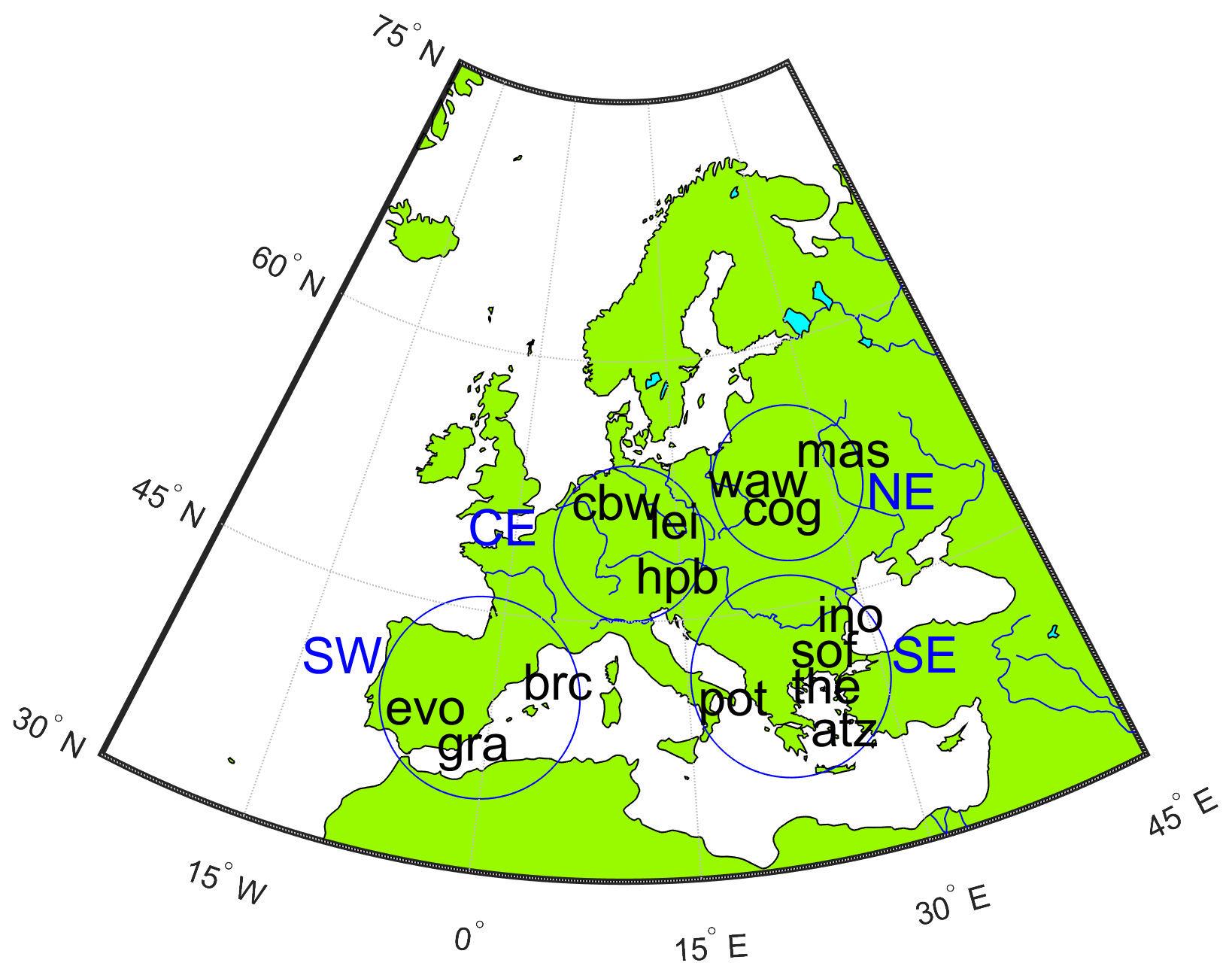
Figure 1 The geographical locations of the 14 stations providing data for the Forest Fire category in the EARLINET database over the 2008–2017 period. The stations are located in Athens (“atz”), Barcelona (“brc”), Belsk (“cog”), Bucharest (“ino”), Cabauw (“cbw”), Evora (“evo”), Granada (“gra”), Leipzig (“lei”), Minsk (“mas”), Hohenpeissenberg observatory (“hpb”), Potenza (“pot”), Sofia (“sof”), Thessaloniki (“the”), and Warsaw (“waw”). The blue circles show the four European geographical regions: south-east (SE), south-west (SW), north-east (NE), and central (CE).

Several stations (Athens, Barcelona, Bucharest, Potenza, Hohenpeißenberg observatory, Thessaloniki, Warsaw) were committed to sending either reprocessed data or to processing additional data using SCC, which were not yet included in EARLINET (most of them for 2017) as of March 2018. Currently (25 June 2020) all of the data are uploaded in the EARLINET database. Within these circumstances, the number of files increased to 3589 (quality control for 2341 files already in the EARLINET database). The diagram of the methodology is shown in Fig. 2. Following the first step in the methodology (Fig. 2), the number of input files (b-files and e-files) for each station is shown in Fig. 3 and Table 1. As a first remark, we can observe that we handle a large variety of lidar systems. Thus, we have one system with 3b + 2e + 2d (Warsaw), three systems with 3b + 2e + 1d (Bucharest, Hohenpeißenberg observatory, and Potenza), five systems with 3b + 2e (Athens, Cabauw, Evora, Granada, and Thessaloniki), four systems with 3b (Barcelona, Belsk, Leipzig, and Minsk), and one system with 1b (Sofia). The total number of b-files and e-files is shown in Table 1. The total number of particle backscatter coefficient, extinction coefficient, and linear depolarization ratio after the first quality checks (EARLINET checks) is βp355 = 969, βp532 = 864, βp1064 = 830, κp355 = 524, κp532 = 503, PDR355 = 131, and PDR532 = 320 (total of 4141 profiles). The distribution by stations follows closely Fig. 3. The stations with the largest contribution for the Forest Fire category are Athens, Bucharest, Granada, Thessaloniki, and Warsaw.

Figure 2 Methodology diagram.

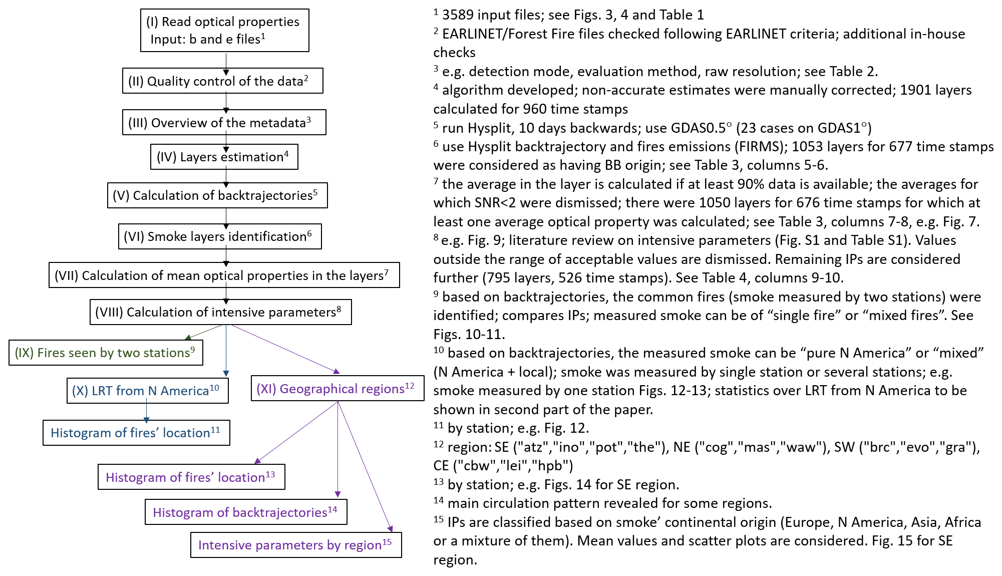
Table 1 List of stations and their number of backscatter (b-files) and/or extinction (e-files) at 355, 532, and 1064 nm. The number of particle backscatter (βp) and extinction (κp) coefficients and particle linear depolarization ratio (PDR) are shown as well. The colour code is as follows: ; or ; ; . b: backscatter, e: extinction, d: depolarization. The last column represents the number of time stamps with at least one profile of optical properties (the total number being 1138).

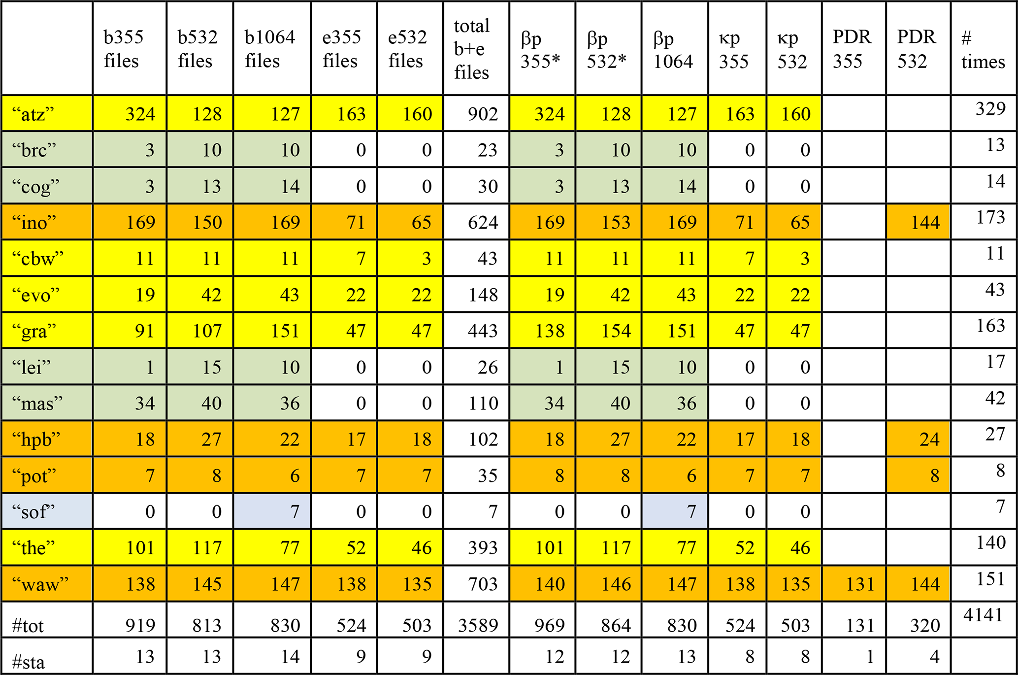
^* Backscatter coefficient profiles from both b-files and e-files; for the same time stamp, the profile from the e-file is kept. Tot: total number of files or profiles; Sta: number of stations with a particular file or profile.

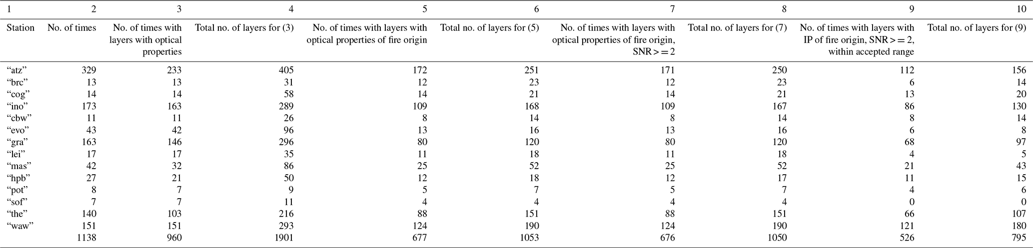
Table 2 (1) Station code. (2) Number of time stamps with at least one profile of optical properties (number of times). (3) Number of time stamps with layers and at least one optical property in the layer. (4) Total number of layers for time stamps in (3). (5) Number of time stamps with optical properties of fire origin. (6) Total number of layers for time stamps in (5). Columns 7 and 8 represent the number of times with good optical properties and the total number of layers with good optical properties. Columns 9 and 10 represent the final number of time stamps and the corresponding number of layers within the imposed acceptable range.

Note that the number of particle extinction coefficient profiles equals the number of “e”-files, while the number of particle backscatter coefficients at 1064 nm equals the number of b1064 files. In the case of particle backscatter coefficients at 355 and 532 nm, their number can be larger than the number of “b”-files as retrievals of backscatter coefficient are reported also in “e”-files employing the use of a Raman channel in the retrieval of backscatter coefficients (using either the Raman method or the aerosol backscattering ratio method). As seen in Table 1, this is the case for the stations Bucharest, Granada, Potenza, and Warsaw. For the same time stamp, the profile from the “e”-file is kept. The reason behind this is that the backscatter coefficient will be further used to calculate the lidar ratio, and the same spatial resolution as the extinction coefficient is desirable. The occurrence in time of the retrievals is shown in Fig. 4. Only the cases for which the layers have a fire origin are shown (smoke layers). As observed, there are sporadic measurements reported for the years 2008–2011. Starting with 2012, more stations started reporting biomass burning pollution events. The total number of time stamps for which we have at least one profile with an optical property is shown in the last column of Table 1.

Figure 3 Number of “b”- and “e”-files available from 14 EARLINET stations providing data for Forest Fire over the 2008–2017 period.

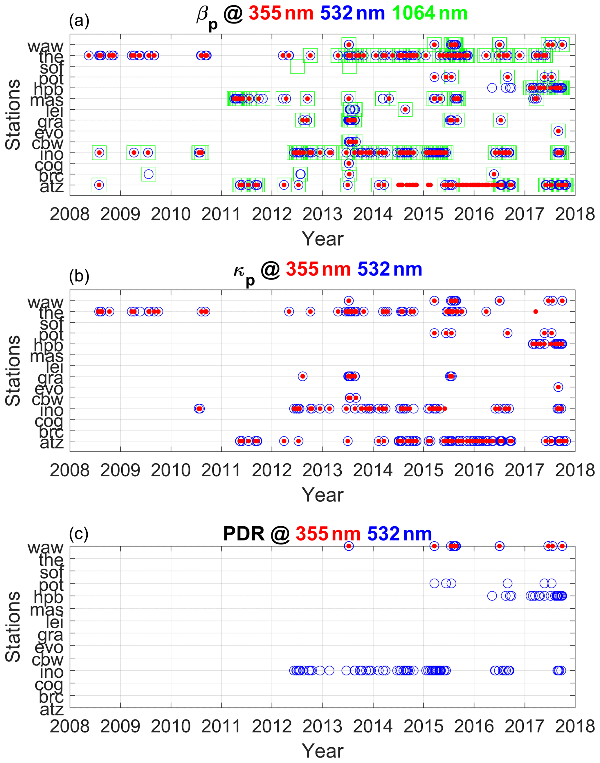
Figure 4 Time span of the available particle backscatter coefficient (a), extinction coefficient (b), and depolarization ratio (c) for each station, over the 2008–2017 period, for the smoke layers.

2.2 Overview of the metadata

Metadata refer to those parameters which give information about the instrument and site location, data processing, or analysing and are saved as general attributes in the “e” and “b” netCDF files. The fixed parameters refer to the measurement position, system name, emission, and detection wavelengths. The dynamic parameters change in time and space: date and time of measurement, raw resolution, time resolution (shots averaged), detection mode, final resolution, and evaluation method. Another two parameters (input parameters and comments) can give additional information (e.g. values used for Rayleigh calibration).

The detection mode (type of data acquisition) can be analog, photon counting, or both (glued signal). The evaluation method (approach used to retrieve the optical properties) can be the Fernald–Klett method (used in b-files to calculate particle backscatter coefficient), the Raman method (used in e-files to determine particle extinction coefficient), and the aerosol backscatter ratio to obtain particle backscatter coefficient using a combination of both elastic and Raman channels (recorded in e-files). The information for parameters is provided in a free-style comment format, and we could not perform the quantification for all parameters (e.g. we could not determine the final spatial resolution or the method used for smoothing and error calculation). In general, there are three approaches reported: (1) keep the errors within an established threshold and thus vary the spatial resolution, (2) maintain a fine spatial resolution (with high statistical errors), (3) perform variable smoothing (e.g. lower spatial resolution above PBL). As expected, the backscatter profiles are less smooth than the extinction profiles.

The summary of the statistics (based on the entire dataset input) over the detection mode, evaluation method, raw resolution, shots averaged, and zenith angle for each backscatter and extinction coefficient is given in Table S2 (Fig. 2, stage III in Methodology). The main features are the following. For b355 and b532 files, the detection mode most employed is the glued signal, while for b1064 it is the analog signal. For e-files, the detection mode most employed is photon counting. The most used evaluation approach for b-files is Klett–Fernald (for particle backscatter coefficient), while for e-files it is Raman (for particle extinction coefficient). Please note that there are 139 cases reported for b1064 which use Raman as its evaluation method (Warsaw station). The station used a PollyXT system, and the algorithm employed to calculate the particle backscatter coefficient at 1064 nm involves the extinction coefficient determined at 607 nm from the Raman signal (no reference is available). Concerning the raw resolution, most of the stations used 3.75 m for backscatter and 60 m for extinction. The zenith angle was mostly 0. The shots averaged were in general tens of thousands. This overview shows that we deal with a variety of approaches to computing the mean profile and associated uncertainty.

3 Data quality control

The first check on data quality consisted of verifying the data which passed the quality control according to EARLINET criteria (Fig. 2, stage II in Methodology). The description of the checks can be found on the EARLINET website (https://www.earlinet.org/index.php?id=125, last access: 26 November 2019). Basically, there are two types of checks. The first check consists of technical checks on the raw data submitted (applied on the fly since June 2018). Here the conformity of the file content is checked with regard to EARLINET file structure and quality control (QC) procedures. With the on-the-fly version, an automatic feedback is provided to the Data Originator reporting all the problems incurred for each rejected file, fostering prompt resubmission of the data (see the 14 June 2018 report at https://www.earlinet.org/index.php?id=293, last access: 26 November 2019). Also, the files not providing the associated error are eliminated. The second check (physical), applied offline, first verifies whether the data were submitted to the right category. Then, the errors are checked for negative value occurrence. Specific checks on backscatter and extinction coefficients are performed (e.g. if larger than a threshold, if integrated quantities such as AOD are within common limits) as well as on intensive variables (where possible), such as LR. The current short description corresponds to the documents issued by 14 June 2018. Three text files are generated with the names of the files rejected by technical criteria (QC_0.0.txt) or passing technical criteria but failing physical criteria (QC_1.0), the files passing both tests being shown in file QC_2.0. After the EARLINET QC tests, there were 2341 out of 3579 initial files (available from 14 stations) that there were passing both tests from (i.e. ∼ 65 %). After adding reprocessed data/newly processed data, the total number of input files increased to 3589.

Several in-house checks (most of them manually performed) were further applied for the selection of good-quality data. Recall that the additional and revised profiles sent by several stations were not on-the-fly QC by the EARLINET procedures. Note that the additional quality checks are performed along various steps during data analysis and are briefly discussed here. The offline QC was manually performed for each profile before applying the algorithm for the layers' detection (Sect. 4.1). Thus, profiles showing atypical behaviour (biased towards negative values, unrealistically increasing above a certain altitude, with PDR outside the [0, 1] range) were dismissed. Sometimes, there were profiles which did not show a clearly defined layer, and thus they were eliminated (Sect. 4.1). The profiles for which no fire was found along the back trajectory were also eliminated (Sect. 4.3). The optical properties in a specific layer were dismissed if the number of available points was less than 90 % and, thus, no mean value was calculated (Sect. 4.4). Values of the mean optical properties for which signal-to-noise ratio (SNR) was less than 2 were also dismissed (Sect. 4.4). Finally, the values of the intensive parameters with SNR < 2 and outside the imposed limits are also excluded (Sect. 4.4).

4 Data analysis

4.1 Calculation of the aerosol layer boundaries

Prior to evaluation of the layer boundaries (Fig. 2, stage IV in Methodology), a manual QC of the profiles of the optical properties was performed. Thus, a number of optical properties profiles which did not show expected realistic behaviour were eliminated. The most common behaviours of the profiles being eliminated are

• profiles showing a large range of negative values due to a systematic error resulting in a bias towards negative values;

• profiles displaying an increase above a certain altitude, most probably due to a non-accurate calibration region;

• depolarization profiles displaying values outside the [0, 1] region; and

• too noisy profiles (SNR < 1).

The algorithm to describe the layers boundaries is described in Sect. S3 of the Supplement.

A few examples of boundary estimation of the (smoke) pollution layers are shown in Fig. S1 in the Supplement. All the optical properties profiles are shown (left – particle backscatter coefficients, middle – particle extinction coefficients, left – particle linear depolarization ratio) in order to get a glimpse of what the layers look like for all profiles. The first plots (a–e) show examples of automatic selection of the layers based on developed algorithm. The first four are based on the b1064 signal, while the fifth is based on the b355 signal. The next plots (f–i) show examples where one or more boundaries are manually modified. The last plot is based on the b532 signal. In example (f) a layer automatically selected around 6500 m was dismissed (considered not substantial), while in example (g) the uppermost layer was manually added. The layers are shown by the grey areas.

Most of the layers detected are situated between 1000 and 5000 m altitude (typically above the PBL). However, the minimum layer bottom was found at 257.5 m, while the highest layer top was found at 19.8 km. Minimum, maximum, and the mean layer thickness were 300, 6862.5, and 1337.5 m. Please note that not all the layers shown here have BB origin (as this check is not performed yet).

The optical profiles shown in Fig. S1 to illustrate the layer estimation also show various questionable patterns for different optical variables. Our quality checks were meant to eliminate profiles (or parts of profiles) where suspicions arise. The examples shown in (a), (b), and (h) were eliminated as they were considered to be of non-BB origin (as discussed later). For the profiles in (c), all layers have BB origin. Various QCs did not allow the estimation of the IPs based on a non-reliable backscatter coefficient at 355 nm for the second and third layers, while PDR@355 was dismissed as well. For the (d) case, both layers have BB origin. QC did not allow the retrieval of various IPs based on non-reliable backscatter coefficient at 355 nm. For the (g) case, the first layer was considered to have a BB origin. QC did not allow the computation of the mean PDR in the layers. For the (i) case, all three layers have BB origin. However, the QC allowed the estimation of both LR and EAE for first layer and only EAE for the second layer.

4.2 Calculation of the back trajectories

Even if the lidar data were stored within the Forest Fire category in the EARLINET/ACTRIS database, in many cases there are situations when several aerosol layers are present and not all of them have a BB origin. Thus, we would like to differentiate these cases and eliminate the non-smoke layers from analysis.

Matlab and Python routines were used to automatically obtain the back trajectories using Hysplit. The settings for the Hysplit backward run are the following: input altitude (middle of the layer) is provided about sea level (a.s.l.), run time is 240 h, the meteorological model is GDAS at 0.5^∘ resolution, and vertical motion is chosen as model vertical velocity (Fig. 2, stage V in Methodology). The terrain height is saved in the output text file. For 23 cases (during August 2010, 2012, and 2013), the GDAS meteorology was not available at 0.5^∘ resolution and, thus, a manual run was performed using a resolution of 1^∘. For the situations when more than three layers were available for a profile, Hysplit was run more than one time. There were 75 such cases. We performed 1036 Hysplit runs for 1901 layers corresponding to 960 time stamps.

The Hysplit back trajectory is the most used tool to track the air-mass origin. For the literature review of BB, 30 papers made use of Hysplit (references 5, 6, 10–12, 14–21, 23, 24, 28–44, and 46 in Table S4, Sicard et al., 2019), whereas five studies use Flexpart (references 2–4, 24, and 26 in Table S4). The running time used in Hysplit simulations reported in the literature varies from 2 to 10 d.

4.3 Layer identification based on back trajectories and fire emissions

The output from the Hysplit text files and the information about fires taken from FIRM MODIS (https://firms.modaps.eosdis.nasa.gov/, last access: 26 November 2019) were used to produce the combined plots containing information about both the fires' presence and the back trajectory (Fig. 2, stage VI in Methodology). The fires are represented in the plots as a function of their fire radiative power (FRP), using different colours and sizes (see legend). The location of the trajectory, each 24 h backwards, is shown by the number of hours. The lower plot shows the altitude a.s.l. of each back trajectory versus time. The fires are chosen within 100 km and within ±1 h around trajectory points (back-trajectory data are available at 1 h temporal resolution). In other words, we assume that those fires are more likely to contribute to the transported smoke, recorded by the lidars. When no fire is recorded along a trajectory, we catalogue that layer as being of non-biomass burning origin (dismissed from further analysis). As a consequence of this criterion, a total of 283 time stamps were considered to have layers with non-BB origin. For many cases, for the same time stamp, there were equally layers of BB origin and non-BB origin. We obtained a number of 678 Hysplit–FIRMS plots (one for each time stamp). Note that the Hysplit–FIRMS plot (corresponding to a time stamp) contains all available layers with fires detected along the trajectory. Examples of such plots are given at a later stage when discussing specific events (Figs. 12 and 14). Based on these criteria, the number of time stamps and corresponding number of layers with BB origin are shown in columns 5 and 6 in Table 2 (compare with columns 3 and 4).

It is worth mentioning that the Hysplit model does not provide the uncertainty. In order to get a possible uncertainty of an individual trajectory, a trajectory ensemble is suggested (Rolph et al., 2017). We may assume that high uncertainties in the air-mass location may occur particularly over long periods of time (e.g. 10 d), which in conjunction with a fire's location may mean a missed fire or a fire detection that was not contributing to the measurement. Drexler (https://www.arl.noaa.gov/hysplit/hysplit-frequently-asked-questions-faqs/faq-hg11/, last access: 26 November 2019) mentions that the uncertainty is between 15 % and 30 %. On the other hand, FIRMS may miss some fires (especially in a cloudy atmosphere). According to Giglio et al. (2016), the collection 6 MODIS has a smaller commission error (false alarm) as compared with Collection 5 (1.2 % versus 2.4 % respectively). The probability of fire detection (regionally) increased by 3 % in boreal North America while staying almost the same in regions such as Europe or northern Africa. We have been using fires with a confidence level larger than 70 %. We did not investigate the injection height based on FRP in order to estimate whether the smoke of a particular fire indeed reached the altitude of the back trajectory. We would like to emphasize that, due to the satellite's polar orbit, the same geographical location can be seen four times a day at the Equator and more times as the latitude increases (due to orbit overlap). Thus, we may miss a certain number of fires (which burn less than a few hours, between the two orbits). However, we may consider those short-lived fires to be insignificant in smoke production.

The FIRMS database was used in several studies to identify the BB origin. However, all fires occurring over certain periods (for which the back trajectories were calculated) are typically accounted for. Thus, fires occurring over the whole day (e.g. Nicolae et al., 2013; Stachlewska et al., 2018; Janicka et al., 2017) or several days (e.g. Mylonaki et al., 2017; Heese and Wiegner, 2008; Tesche et al., 2011) were reported. By contrast, our novel approach accounts only for those fires which were occurring around a back trajectory (100 km radius) at the time of air-mass passage (±1 h).

4.4 Calculation of the mean optical properties and intensive parameters inside the layers

After determining the aerosol layers and their boundaries (Sect. 4.1–4.3), the mean value of the optical properties is computed for each layer (Fig. 2, stage VII in Methodology). Note that the first and last 50 m of each layer were not considered for the calculation (cf. Nicolae et al., 2018). The uncertainty for each mean value was computed following the error propagation. The mean value in the layer was calculated if there were at least 90 % of the points available (the ratio between the layer depth and the resolution in the layer). There were many cases for which the extinction coefficient or the linear particle depolarization ratio could not be calculated as typically their profiles have a shorter extent than that of a backscatter coefficient. A visual check is performed as well and, thus, where the profiles were suspicious, the mean values in the layers were manually set to NaN.

The SNR was computed as the ratio of the mean value to its uncertainty (e.g. Nicolae et al., 2018). The values of each optical property for which SNR < 2 were dismissed. In Table 2 (columns 7 and 8), we show the number of the time stamps and the layers with a good SNR for optical properties. As a result of this criterium, only one time stamp was dismissed (Athens), and three layers (one for each of Athens, Bucharest, and the Hohenpeißenberg observatory). Please keep in mind that the number of dismissed optical properties in layers is larger than the number of dismissed layers, as one layer is dismissed only when all optical properties in the layers are discharged.

Figure S2 shows an example (for Athens) of the number of layers selected and the corresponding number of optical properties evaluated in each layer. For this example, we have 171/172 time stamps, from which we could determine 250 layers. It was just one layer for which we could not determine the optical properties due to SNR constraint (see columns 5–8 in Table 2).

Figure 5 Values of the mean optical properties and associated uncertainties in the layers. Example for the Bucharest (“ino”) station. Layers were identified as having a fire source. Note that with few exceptions the uncertainties are very small and thus undiscernible from the mean values.

An example of the mean optical properties computed in the layers (versus measurement time) is given in Fig. 5 for the Bucharest station. The range of values taken by different variables is large. Another aspect is the lower number of values reported or retrieved for extinction and depolarization (these features are specific to all stations). The figures for all the stations will be shown in the companion paper. Systematic measurements and more intensive parameters were available for the Athens, Bucharest, Thessaloniki, and Warsaw stations, while over the entire analysed period, systematic measurements were provided by Athens, Bucharest, and Thessaloniki.

Once the mean optical properties were calculated, the intensive parameters were determined where possible (Fig. 2, stage VIII in Methodology). All the IPs have SNR > 2. The imposed limits (data filtering) for IPs are the following: LR@355 = [20, 150] sr, LR@532 = [20, 150] sr, EAE = [−1, 3], BAE@355/532 = [−1, 3], BAE@532/1064 = [−1, 3], PDR@355 = [0, 0.3] and PDR@532 = [0, 0.3] (following closely Burton et al., 2012; Nicolae et al., 2018). The figures representing the intensive parameters for all the stations will be shown in the companion paper. The collected records of intensive parameters found in the literature (46 reference values from 39 cited papers) are shown in Fig. S3 and Table S3 in the Supplement. Table S4 shows the cited references. The extreme values for LR@355 are 21 sr (Müller et al., 2005) and 130 sr (Tesche et al., 2011), while for LR@532 they are 26 sr (Müller et al., 2005) and 147 sr (Mariano et al., 2010). For EAE we have 0 (Müller et al., 2005) and 2.4 (Giannakaki et al., 2016). For BAE@355/532 we found 0.35 (Tesche et al., 2011) and 2.8 (Giannakaki et al., 2010), while for BAE@532/1064 we found 0.29 (Tesche et al., 2011) and 2.85 (Groß et al., 2013). For PDR@355 the extreme values were 1 % (Janicka et al., 2019) and 31 % (Vaughan et al., 2018), while for PDR@532 the extreme values were 0.3 % (Stachlewska et al., 2018) and 20 % (Hu et al., 2019). Figure S4 shows an example (for Athens) of the number of layers selected and the corresponding number of intensive parameters retrieved. One can compare with Fig. S2 over the difference between the available number of optical properties and the final number of intensive parameters. An example of the intensive parameters is shown in Fig. 6 for the Warsaw station. For the Warsaw site, all profiles for extinction and backscatter were calculated using the classical Raman evaluation (Ansmann et al., 1992). The lines in magenta and cyan represent the minimum and the maximum as reported in the literature.

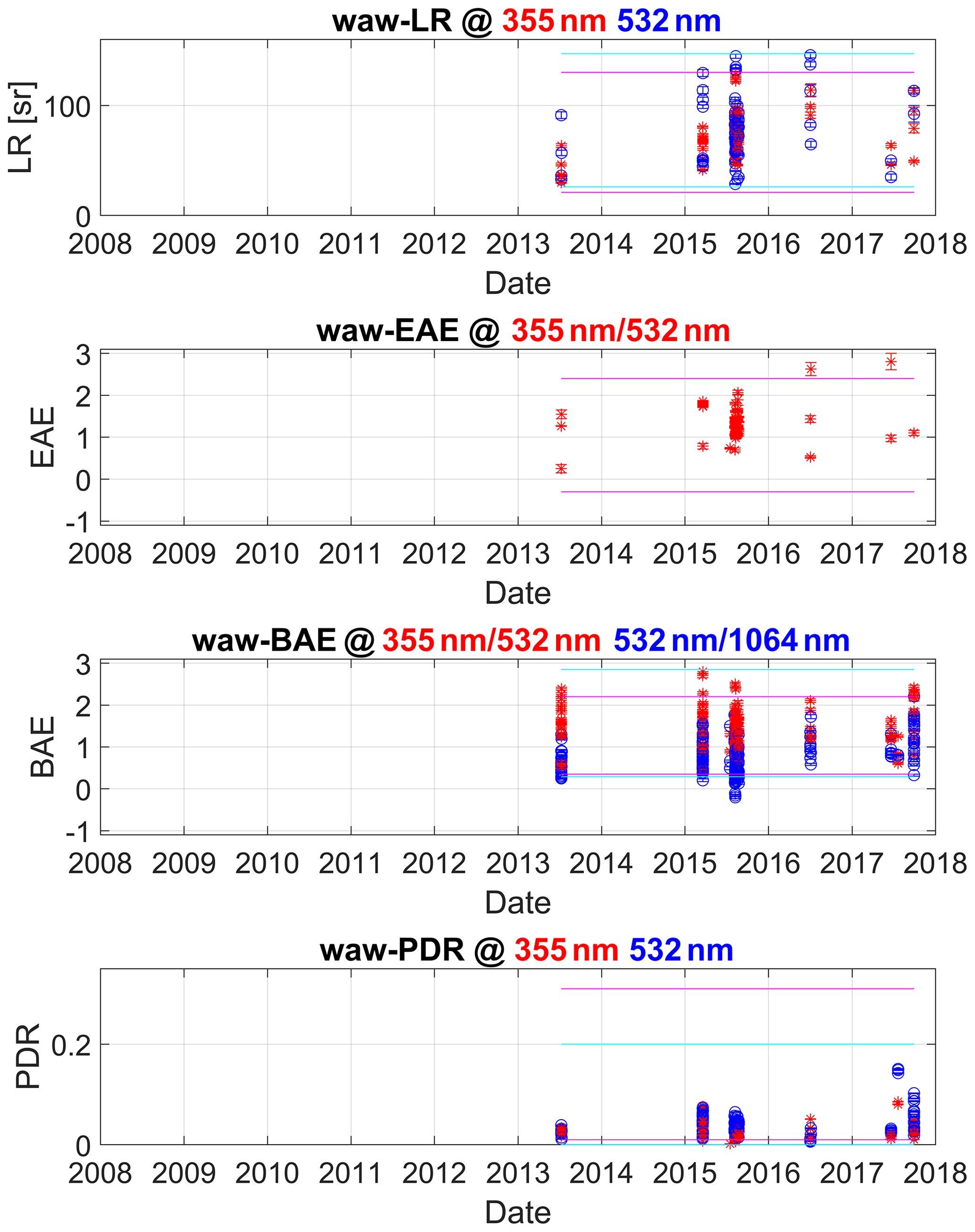
Figure 6 Intensive aerosol parameters derived in the layers. Example for Warsaw (“waw”) station. The lines represent the minimum and maximum values reported in the literature. Magenta lines represent the extreme values for the intensive parameters shown in red, while the cyan lines represent the extreme values for the intensive parameters shown in blue. Layers have fire source origin.

In general, LR, EAE, both BAEs, and PDR are spread well within the reported limits, although the latter is rather in its lower range. Lower PDR may be explained as due to the specific location of Warsaw being much closer to BB sources in Ukraine, Belarus, and Russia than other EU countries and therefore much more exposed to faster and more direct BB transport to this site. In such a case, differences of properties with respect to other measurement sites in Europe are expected and revealed within our work. Moreover, Warsaw is much less exposed to mineral dust intrusions, in comparison with many EU sites at which the BB measurements are more likely to be affected by slight contamination of dust, e.g. Spanish sites. On the other hand, Warsaw is an urban site, and thus for BB observed in layers at lower ranges a slight contamination of the BB with the local urban pollution is possible. For higher layers, industrial pollution from the Silesia region in Poland (Stachlewska et al., 2018) or the Ruhr region in Germany (e.g. the case here on 4 July 2016 at 07:30) is possible. This can explain a few values outside the literature range observed in Warsaw, i.e. for EAE (2 values), for BAE (33 values), and for PDR355 (8 values). The extreme values for EAE observed on 4 July 2016 07:30 and 19 June 2017 20:30 (2.6 and 2.8 respectively along with CR_LR < 1) correspond to fires in Germany/Belgium and the United Kingdom respectively. The fires occurred in less than 40 h before smoke measurements, and thus we can consider the smoke relatively fresh.

The mean, median, minimum, and maximum values taken by the intensive parameters for all the stations providing at least one parameter (all stations but Sofia) are discussed in the companion paper. The final number of selected layers and the corresponding time stamps are shown in Table 2, columns 9 and 10. The range of values taken by a specific parameter is large. The number of outliers dismissed based on predefined ranges of acceptable values for each intensive parameter is small (3.7 % per total). For each IP we have the following numbers: 8∕305 (2.6 %) for LR@355nm, 8∕253 (3.2 %) for LR@532nm, 18/243 (7.4 %) for EAE, 39/642 (6.1 %) for BAE355/532, 21∕706 (3 %) for BAE532/1064, 0∕132 (0 %) for PDR@355, and 0∕242 (0 %) for PDR@532. Please note that a thorough investigation of the outliers was not performed. Conversely, we focused on a semi-automatic evaluation by applying different criteria for outlier elimination (filtering). One can see three possible reasons for the presence of outliers: (a) the smoothing applied on the Raman signals, which induces a very smooth profile for extinction coefficients, (b) a shift of the profile towards higher altitude (most probably due to a non-accurate calibration range), and (c) a slight difference between the peaks of the backscatter versus extinction or a small difference in the slope (most probably related to the smoothing of the Raman signals). All values of the intensive parameters will be shown in the companion paper. After outlier elimination, we start the data (IP) interpretation.

5 Data interpretation

We have focused on several directions to investigate and interpret the measurements by means of the intensive parameters. Here we show examples for each direction, while a comprehensive analysis will be performed in the following paper.

The following results were found in the literature regarding the IP values versus travel distance (time travel).

• Effective radius: according to Müller et al. (2005, 2007, 2016), the effective radius of the BB particles increases with time (distance), most probably due to coagulation and aggregation of the particles (Reid et al., 2005). Measurements and retrieved values of effective radius of BB particles showed that the fresh particles have a mean radius around 150 nm, while the aged particles have a radius around 300–400 nm (Müller et al., 2007). Particle size depends on many factors, such as the combustion type in fires (in-flame or smouldering) or type of vegetation, while the smoke aerosol undergoes different physical–chemical processes in the atmosphere (Reid and Hobbs, 1998). While the heaviest particles will sediment during transport, the particles reaching the measurement site are still larger than the emitted ones.

• EAE decreases with time (distance) (e.g. Müller et al., 2005, 2007, 2016).

• Lidar ratio: it was shown that for aged BB particles (big travel time), LR@532 > LR@355 (e.g. Wandinger et al., 2002, Murayama et al., 2004; Müller et al., 2005; Sugimoto et al., 2010, Nicolae et al., 2013), hence the colour ratio (CR) for LR, i.e. CR_LR > 1 for aged smoke (LR@532 increases more with aging smoke).

• PDR@532 decreases with time (Nisantzi et al., 2014).

The general correlations between IPs were shown.

• In general, LR532 increases with increasing LR355 (e.g. Nicolae et al., 2018; Janicka and Stachlewska, 2019).

• In general, PDR532 increases with increasing PDR355 (e.g. Stachlewska et al., 2018; Janicka and Stachlewska, 2019).

The following differences between smoke properties in different regions were reported.

• Smoke particles from Brazil absorb more and scatter less the solar radiation as compared with smoke in North America (Reid and Hobbs, 1998).

• Differences between North American and Siberian smoke over Germany: particles from North America showed smaller size and higher EAE (Müller et al., 2005).

The following studies showed different behaviour of BAE versus EAE.

• Veselovskii et al. (2015) tried to relate BAE to EAE and showed that while EAE depends mainly on particle size, BAE depends on both particle size and refractive index, being very sensitive to the latter (see their Fig. 20). On the one hand, when the real part of the refractive index increases, the imaginary part is constant, the effective radius for coarse mode and the high fine-mode fraction are constant, and the effective radius of the fine particles decreases and BAE@532/1064 decreases (BAE@355/532 increases) with increasing EAE (over the ∼ 0.5–1.5 region) (see their Figs. 20 and 22). On the other hand, for a constant refractive index, a fixed effective radius for coarse mode, and an increase in the fine-mode fraction, both BAEs increase with increasing EAE (over the ∼ 0.5–1.5 region). This is visible for different effective radii for the fine particles (see their Fig. 19).

• Su et al. (2008) showed a few scenarios for the relationship between BAE@532/1064 and EAE@553/855, which depend on RH (relative humidity) and the contribution of the fine-mode fraction. For a high fine-mode fraction in the smoke composition and RH < 85 %, BAE@532/1064 increases with increasing EAE@553/855 (EAE > 2). For a dominant coarse mode and RH < 85 %, BAE@532/1064 decreases with increasing EAE@553/855 (EAE < 0.5) (see their Fig. 8). For RH > 85 there is no clear pattern of BAE with respect to EAE (BAE increasing and then decreasing with increasing EAE).

Concluding the findings so far, we expect CR_LR > 1, small values of EAE (<1.4), and smaller PDR@532 for aged smoke (especially for long-range transport from North America). The studies showed no straightforward pattern for CR_BAE and CR_PDR evolution with time. Studies by Veselovskii et al. (2015) and Su et al. (2008) may help interpret the scatter plots between BAE and EAE. We did not investigate the RH field though.

5.1 Fire events seen by several stations. Example for the Bucharest and Thessaloniki stations

Over the 10-year period, we have found five events (with retrieved intensive parameters) recorded at two stations which have the same smoke origin (Fig. 2, stage IX in Methodology). The events belong to local fires in Europe. Two events are seen by the Athens and Thessaloniki stations (2014 and 2017) and one event is seen by the Bucharest and Thessaloniki (2014), Minsk and Warsaw (2015), and Athens and Hohenpeißenberg observatory (2016) stations. Unfortunately, we did not obtain common intensive parameters for all events. Only two events had one common intensive parameter (BAE@532/1064). One event is shortly presented below, emphasizing the methodology.

The event was recorded on 9 and 10 September 2014 at the Bucharest and Thessaloniki stations (see time frame and altitude in Fig. 7a). The back trajectories revealed the same fire origin. Figure 8 shows the air back trajectories for the layers detected at the two stations. The fire's location (within 100 km and ±1 h) is shown as well. The colour and size of the fires correspond to their FRP (see legend). The Hysplit back trajectories in Fig. 8 show that the main smoke source was the fires over eastern Ukraine. Figure 8a (Bucharest station) indicates as a second smoke source the fires over eastern Romania (∼ 72 h back) and northern Ukraine (∼ 144 h back). The smoke particles were transported from Ukraine to the Bucharest station over a period of 5 d, descending from approximately 4200 m on 4 September 2014 to 3000 m on 9 September 2014. For the Thessaloniki station the main source was the fires over south-western Ukraine (Fig. 8b). The smoke particles were identified on 10 September 2014 around 2100 m. Note that for the Thessaloniki case, the “common fire” was detected at ∼ 3500 m. In Fig. 7a–b we show the location of the fires which contributes to all measurements on 9–10 September and their histogram occurrence on 1 × 1 grids. From such histograms we pick the grids where we have fires contributing to both stations. See the grid which has both colours, between 36 and 37 east and 47 and 48 north (also marked by a square in the upper plot). The location (longitude and latitude) of these fires from the “common” grid are shown versus fires occurrence time as well as versus measurement time at each station (Fig. 7c–d). The common fire revealed through the back trajectory occurred at 10:39 on 4 September (latitude = 47.537, longitude = 36.275), and it was recorded at ∼ 11:00 on 9 September at Bucharest and at ∼ 11:00 on 10 September at Thessaloniki (lower layer left). Two layers were detected at the Thessaloniki station (where one corresponds to the common fire) and one at the Bucharest station. We analysed whether there were other fires contributing to the same measurement as, in general, along back trajectories, we encounter many fires at several locations. In the case of Bucharest there were 24 other fires (detected 46 times) contributing, located in Ukraine as well as in north-eastern Romania (occurring on 3, 4, and 6 September). For Thessaloniki we counted 35 other fires (detected 66 times), located in eastern Ukraine (occurring on 2 and 4 September). See Fig. 8b. Please note that as a function of the air trajectory, one fire can be seen more than once (e.g. during a cyclone or anticyclone) or due to slow air motion (spatial–temporal stationarity over the 100 km area and 1 h).

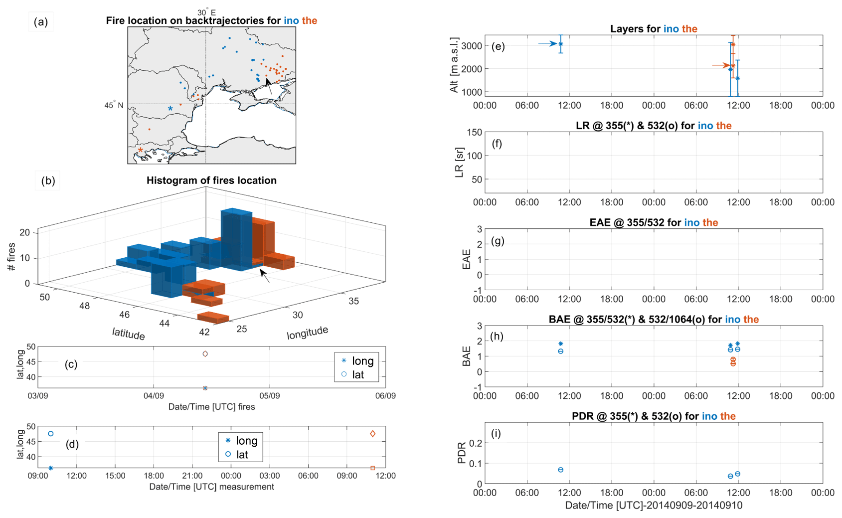
Figure 7 Measurements with the same source in Thessaloniki (“the”) and Bucharest (“ino”) on 9 and 10 September 2014. (a) Fire locations seen during back trajectories from each station (colour coded). (b) Histogram of the fire occurrence in each geographical grid. (c) Longitude and latitude of the common fire location versus fire occurrence time. (d) Longitude and latitude of the common fire location versus measurement time at the two locations. (e–i) Smoke layer altitude and intensive parameters for each station. Layers measuring the common fire are shown by arrows. The geographical location of the common fire is shown in the histogram by an arrow.

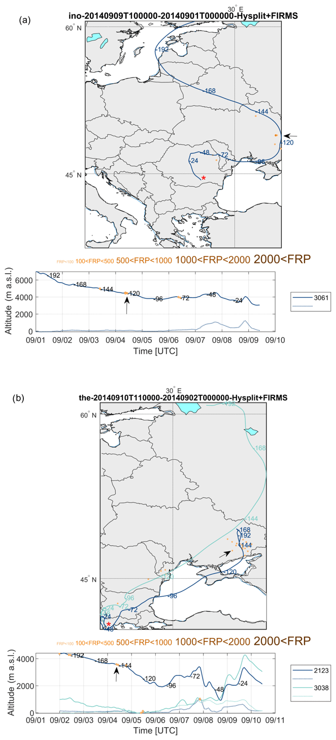
Figure 8 Back trajectories and locations of fires along back trajectories within 100 km and ±1 h for Bucharest (“ino”) on 9 September 2014 (a) and Thessaloniki (“the”) on 10 September 2014 (b). Lower plots show the altitude (a.s.l.) of the back trajectories versus time. The common fire location is marked with an arrow. See text for more details.

We can conclude that we have a mixed smoke recorded in both Bucharest and Thessaloniki. However, the mixtures are different for the Bucharest and Thessaloniki stations.

Figure 7e–i show the layer locations (marked by an arrow in front of the middle of the layer) and intensive parameters for the layers. Note that the retrieval of the intensive parameters was not possible at all times for all layers. The two layers detected in Bucharest and Thessaloniki were located at 3061 and 2123 m respectively.

For the measurements at the Bucharest (9 September 2014 10:45 UTC) and Thessaloniki (10 September 2014 11:15 UTC) locations, which correspond to the common fire in eastern Ukraine (47.537^∘ N, 36.275^∘ E) on 9 September 2014 10:39 (as well as other additional fires for each station), the following intensive parameters were calculated.

Bucharest, 9 September 10:45, 3061 m: BAE@355/532 = 1.82 ± 0.0001, BAE@532/1064 = 1.32 ± 0.0001, PDR@532 = 6.8 ±  0.03 %.

Thessaloniki, 10 September 11:15, 2123 m: BAE@532/1064 = 0.51 ± 0.02.

The values for BAE@532/1064 were 1.32 and 0.51 for Bucharest and Thessaloniki respectively. The difference between the two values may be explained by the different mixtures of smoke (originating from different fires). All the contributing fires for Thessaloniki besides the common fire are located in eastern Ukraine, while the contributing fires for Bucharest are located in eastern Romania, eastern Ukraine, and north-eastern Ukraine. According to back trajectories for Thessaloniki, the other fires contributing to measurements are further located in time than the common fire. A lower value for BAE@532/1064 in Thessaloniki reveals a relatively larger contribution of the big particles to backscatter. By contrast, in Bucharest the smallest particles show the highest backscatter coefficient.

For the other event with a common IP for the same source (29 May 2017–2 June 2017), the smoke was labelled as of a “single fire” as no other fires were identified along the back trajectory. The common fire occurred on 26 May at midnight in Ukraine (48.171^∘ N, 30.622^∘ E) and it was recorded in Thessaloniki and Athens on 29 and 31 May respectively. The BAE@532/1064 value in Thessaloniki was less than half of that in Athens, while BAE@355/532 was larger for Thessaloniki. High BAE corresponds to higher backscatter at the smaller wavelengths, which indicates a higher number of small particles. The values in Thessaloniki correspond to a higher number of small-size particles (at 355 nm) and to a higher proportion of large particles (at 1064 nm) compared with Athens. CR_BAE (colour ratio of the backscatter Ångström exponents) increases from Thessaloniki to Athens (0.22 to 0.78 respectively), which suggests an increase with travel distance (time). As CR_LR (colour ratio of the lidar ratios) and EAE (extinction Ångström exponent) were not available to characterize the smoke in terms of age, we classified the smoke as aged based on the duration of the travel time.

Overall, we conclude that the number of common events as well as the number of the common IPs is limited and, thus, no thorough examination of these events is possible. The most important feature of this analysis is that it enables us to quantify the smoke as being “single fire” or “mixed” and hence explain various IP values. This kind of analysis can be successfully applied in the future, when more data become available.

5.2 Long-range transport from North America. Example for the Athens station

We have identified a total of 24 events with long-range transport from North America (Fig. 2, stage X in Methodology) for which we have at least one intensive parameter retrieved. The events are reported in 2009 and over the 2012–2017 period. As in the previous section, for each event, we plot the Hysplit trajectory and the location of the fires along it, the histogram with the number of fires in each ${\mathrm{1}}^{\circ }\times {\mathrm{1}}^{\circ }$ geographical grid, the geographical location (longitude and latitude) versus occurrence time of the fires, and versus measurement time at the stations(s). Last, we show the layer's altitude (error bar signifies the layer's thickness) and the intensive parameters in the layers.

We have identified eight measurement periods (events) when the smoke is arriving solely from North America (“pure N America”). The other cases represent measurements of mixed smoke, where the smoke is coming from both North American and local fires (mostly European) (“mixed”). In two cases we have mixed smoke from North America and northern Africa or the Middle East. Usually, during measurements period, there were also recordings of BB with other origin (Europe). For each layer we check whether the smoke is coming from a single fire or more fires (count their number) and quantify the locations. We have one event when there were measurements taken at three stations and one event with measurements taken at two stations. All the other cases represent measurements recorded by a single station. As the number of intensive parameters determined for each station varies considerably, in general we cannot compare directly all IPs for the same event. As a consequence, a statistical analysis will be performed over the entire set of parameters. Below we show one example of long-range transport recorded in Athens which provided more measurements and more intensive parameters. The event recorded over 3 d in July 2013 will be discussed in the companion paper.

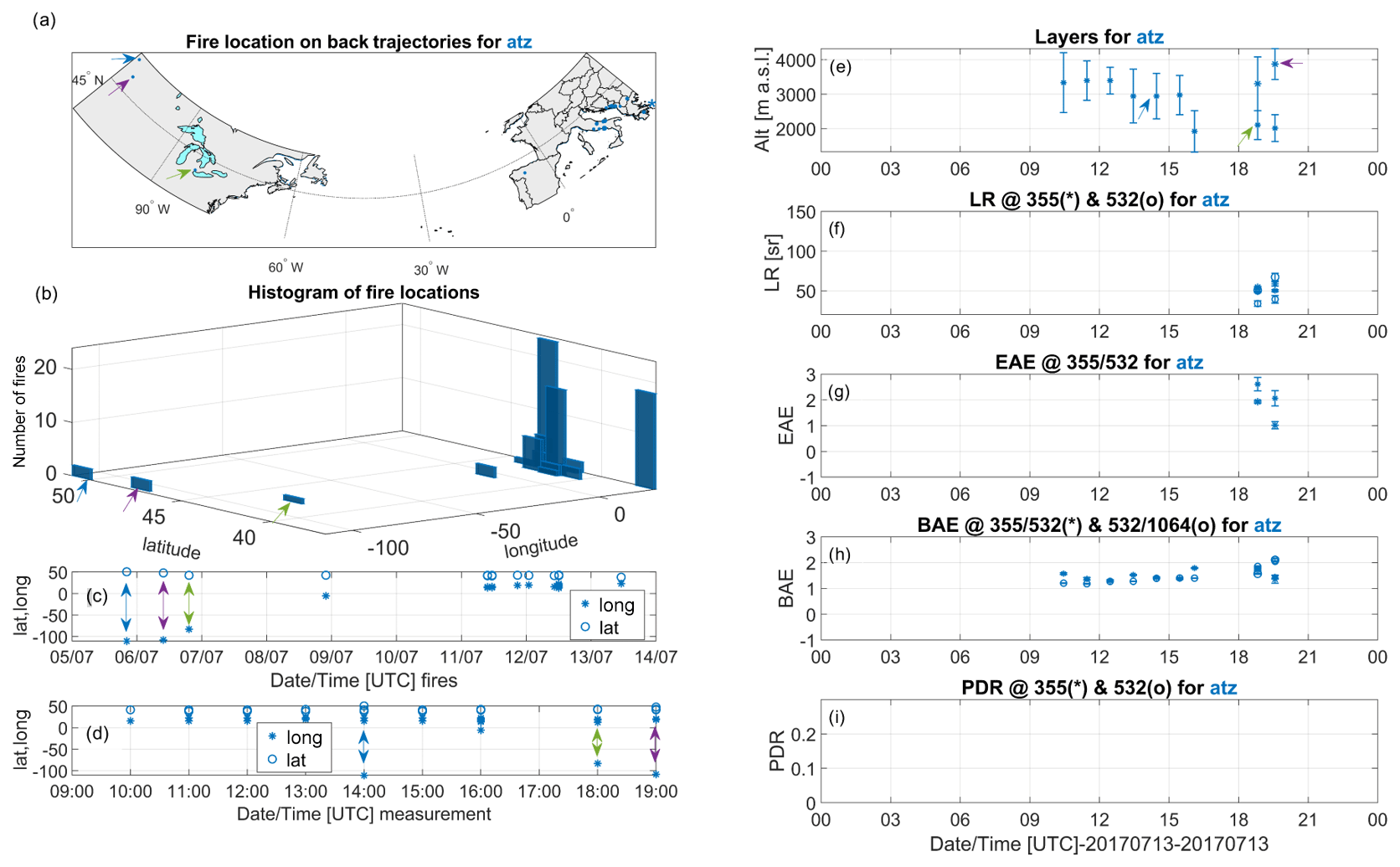
Figure 9 LRT as measured at Athens (“atz”) on 13 July 2017. (a) Locations of the fires. (b) Histogram of the fire occurrence in each geographical grid. The North American fires are marked by arrows. (c) Fire coordinates versus fire occurrence time. (d) Fire coordinates versus measurement time. (e) Smoke layer altitude. Layers measuring LRT smoke are marked by arrows. The first two smoke layers are considered “mixed” and the third (magenta) “pure NA”. (f–i) Intensive parameters.

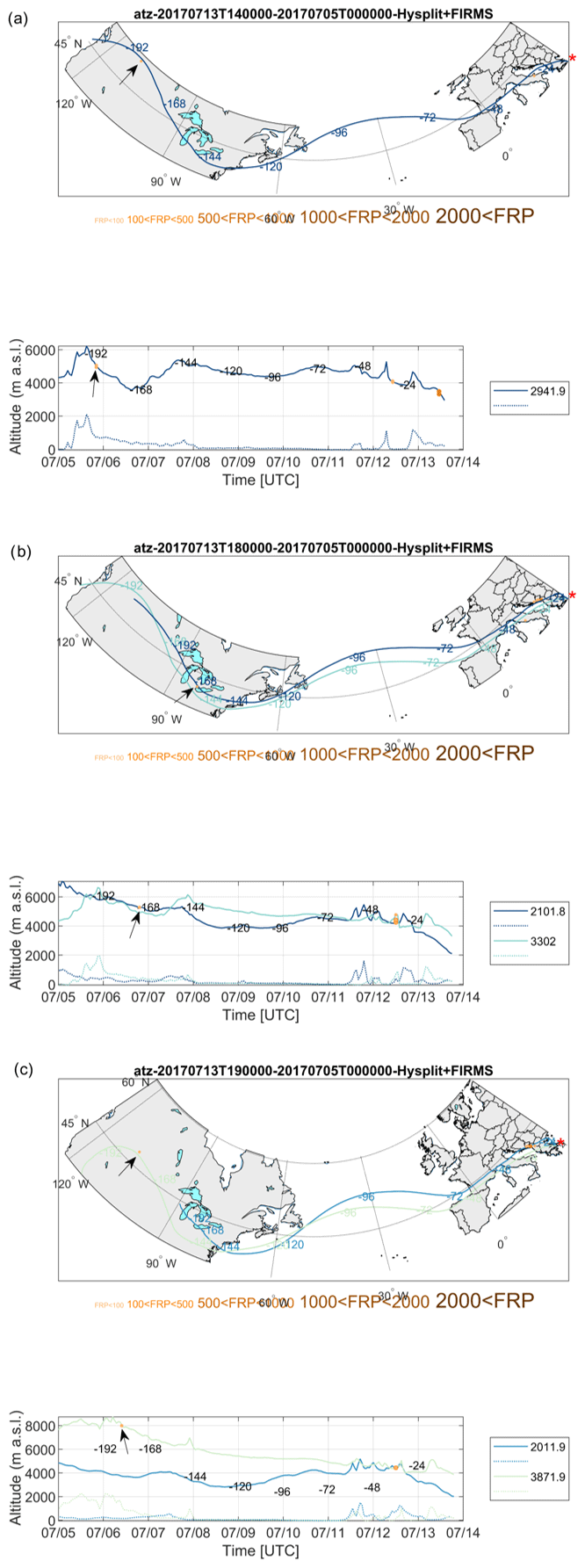
Figure 10 Back trajectories for layers shown in Fig. 9 for the Athens (“atz”) station. Layers in (a) and (b) are considered “mixed”, while the layer in (c) is considered “pure N America”. See text for more explanation. The fire location is marked with an arrow.

5.2.1 Smoke event recorded on 13 July 2017

During this day we recorded several measurements in Athens (see time and layer altitude in Fig. 9e). According to the back trajectory and the fire occurrence along it, we determined three layers of North American smoke origin (their location is marked with a black square on the left). As seen in the back trajectory (Fig. 10), the fire locations in North America are different for the three layers (different sources).

The first layer of smoke origin was detected at 14:27 at ∼ 2900 m altitude. Our calculations show that there were different fires contributing to this measurement. Thus, we have four fires (counted eight times), of which only one fire (counted twice) was of North American origin. This can be seen in Fig. 9d as well as in the back trajectory in Fig. 10a, where we see the fires detected in the first 2 d backwards (local fires, in Greece and Italy) as well as the fire found after almost 8 d back in North America. The fire from North America occurred at 20:14 on 5 July in the longitude-by-latitude grid [−111, −110] × [50, 51]. The location of the fire is shown by blue arrows in Fig. 9a–e.

The second layer was measured at 18:49 at 2102 m altitude. Twelve fires were found (counted 19 times) to have contributed to the measurement, of which one fire (detected once) was of North American origin. See Figs. 9 and 10. The fire from North America was detected at 19:16 on 6 July in the longitude-by-latitude grid [−84 −83] × [42, 43]. The location of the fire is shown by green arrows in Fig. 9a–e.

The last layer was measured at 19:34 at 3872 m altitude. We found two fires (each detected once) of North American origin. The North American fires occurred at 09:47 on 6 July and were located in the longitude-by-latitude grid [−109, −108] × [47, 48]. The location of the fire is shown by magenta arrows in Fig. 9a–e. The trajectory layer in Fig. 10c is the higher one (light blue). The local fires observed in the plot are detected by the first layer (at 2012 m).

Thus, we can label the first two layers as “mixed” smoke and the third one as “pure N America” smoke. We observe that for the mixed fires, the contribution from local fires is much larger as we have 6∕8 and 18∕19 fire counts in Europe for the first and second layers respectively. The intensive parameters for the three layers are

• layer 1 @ 14:27 2942 m, mixed: BAE@355/532 = 1.42 ± 0.03, BAE@532/1064 = 1.39 ± 0.01;

• layer 2 @ 18:49 2102 m, mixed: LR@355 = 48.4 ± 1.04 sr, LR@532 = 33.7 ± 3.5 sr, BAE@355/532 = 1.72 ± 0.05, BAE@532/1064 = 1.85 ± 0.02; and

• layer 3 @ 19:34 3872 m, North America: LR@355 = 58.5 ± 2.63 sr, LR@532 = 67.2 ± 4.79 sr, EAE = 1.02 ± 0.14, BAE@355/532 = 1.36 ± 0.15, BAE@532/1064 = 2.11 ± 0.08.

We observe that BAE@355/532 has the smallest value for “pure N America”, while BAE@532/1064 has the highest. A relatively small value for EAE for the third layer corresponds to bigger (coarse-mode) particles, associated with aged smoke. On the other hand, values of LR (LR@355 < LR@532) suggest the presence of aged aerosol as well. The layer's altitude is the highest of all three. The values of LR for the second layer (LR@355 > LR@532) suggest fresh aerosol (of smaller-size, fine-mode particles). This can be supported by the contribution of the local fires (detected a few hours back). If we compare the colour ratio (CR) of BAE, we obtain values of 0.98, 1.08, and 1.55 for the three layers. CR_LR for the second and third layers were 0.7 (fresh smoke) and 1.15 (aged aerosol). Based on all reported values in the literature (Table S3), we found the following values for CR_LR and EAE for the fresh, aged, and North American cases (particularly the case of aged smoke). CR_LR was 0.88, 1.08, and 1.23, while EAE was 1.47, 1.2, and 0.95. CR_BAE had the values 0.76, 0.98, and 0.98. We may speculate that CR_BAE may increase with time (distance).

Please note that the time difference (an hour at most) between right plots and bottom left plots comes from the fact that Hysplit back trajectories start at sharp hours. For example, for the measurement at 18:49 the starting point on the back trajectory is 18.

Statistics on LRT from North America will be shown in the companion paper. We encountered 168 measurements over the 24 periods (over the 2009–2017 period). Of these measurements, 77 have a North American origin, while the other 91 have a different BB origin (local). The LRT events from North America are analysed by distinguishing between “pure N America” fires (sensed smoke comes solely from North America) and “mixed” fires (measured smoke is a mixture of North American smoke and local/European smoke).

5.3 Analysis over geographical regions

5.3.1 Geographical regions

Taking into account the position of the 14 stations (Fig. 1), four geographical regions are chosen as follows: south-eastern Europe (Potenza, Athens, Thessaloniki, Sofia, Bucharest), south-western Europe (Granada, Barcelona, Evora), north-eastern Europe (Belsk, Warsaw, Minsk), and central Europe (Cabauw, Leipzig, Hohenpeißenberg observatory). This corresponds to stage XI from Methodology (Fig. 2). The statistics over the measurements for each individual station show the following. The Belsk and Cabauw stations focused on LRT smoke from North America, with ∼ 99 % of the measurements (1149∕1159 and 1001∕1013 North American fires / total number of fires). Leipzig measured 86.2 % (156∕181 North American fires / total number of fires) LRT smoke. The others have measured mostly in Europe as follows (no. of fires in EU / no. of total fires): Athens 81.7 % (1657∕2028), Barcelona 91 % (172∕189), Bucharest 93.82 % (1883∕2007 cases), Granada 68.32 % (1643∕2405), Minsk 98.04 % (1051∕1072), Hohenpeissenberg observatory 74.84 % (116∕286), Potenza 100 % (142∕142), Sofia 100 % (16∕16), Thessaloniki 87.38 % (1807∕2068), Warsaw 85.4 % (5036∕5897). For the Evora station we encountered 44.39 % (99∕223) fires in North America and 48.43 % in Europe (108∕223). Per region, we have detected fires from North America as 4.5 % (282∕6261), 8.56 % (241∕2817), 87.55 % (1181∕1349), and 24.13 % (1961∕8128) for the south-eastern, south-western, central, and north-eastern regions respectively. The number of fires detected in Europe was the following: 87.93 % (5505∕6261), 68.26 % (1923∕2817), 11.34 % (153∕1349), and 75.01 % (6097∕8128) for the south-eastern, south-western, central, and north-eastern regions respectively.

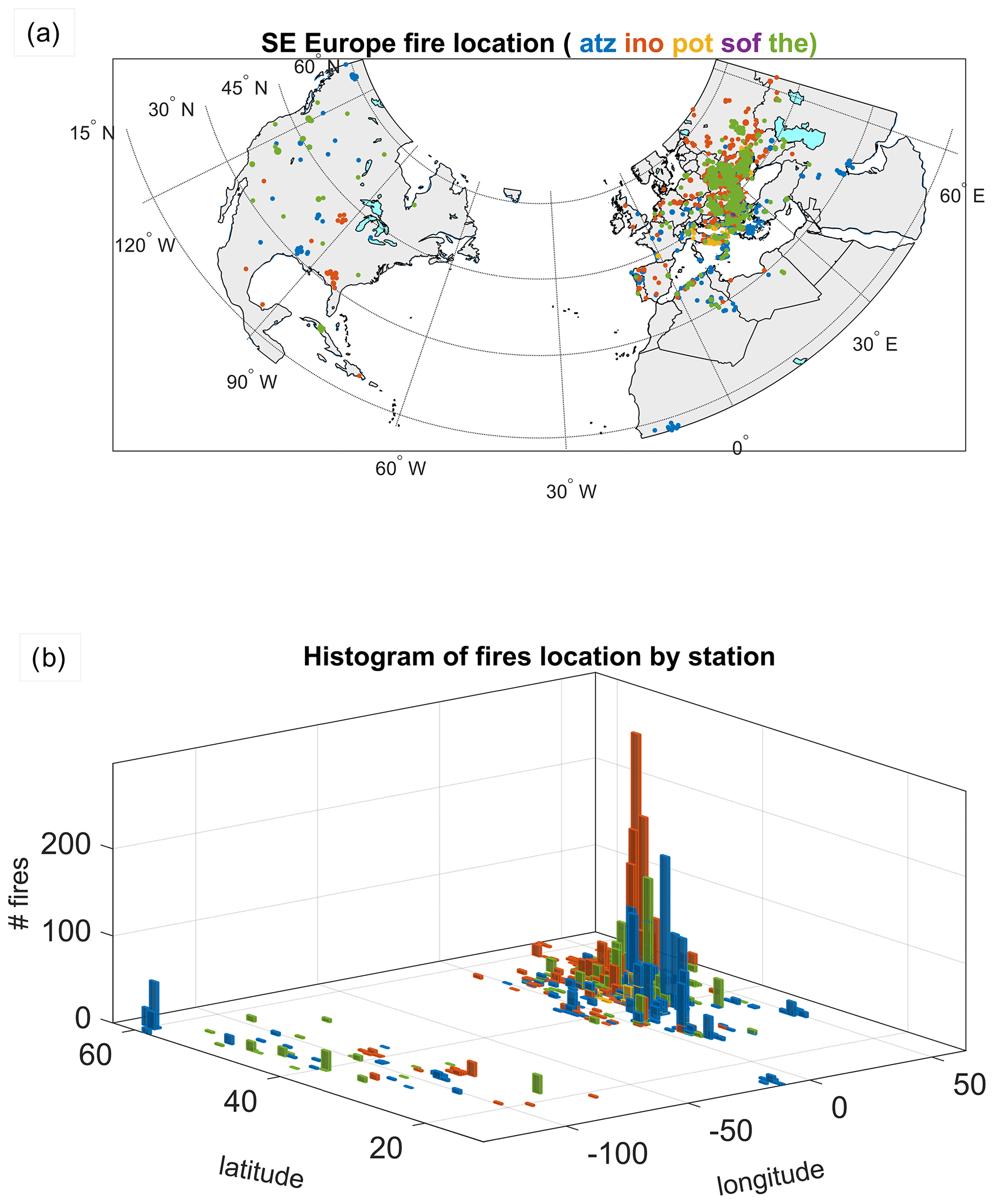
Figure 11 South-eastern European region formed by stations Athens (“atz”), Bucharest (“ino”), Potenza (“pot”), Sofia (“sof”), and Thessaloniki (“the”). (a) Location of the fires detected by each station. Note that due to overlap, some are not seen. (b) Histogram of the fires detected by each station.

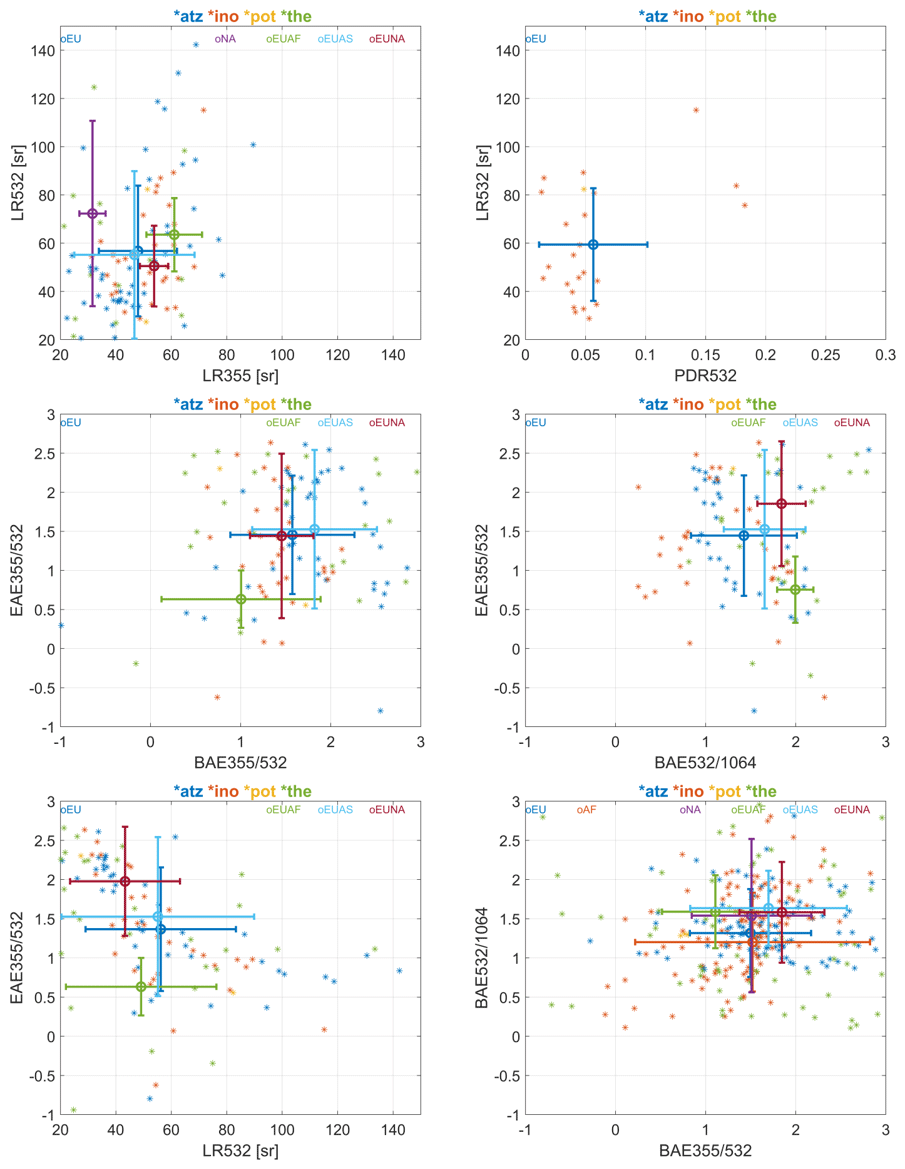
Figure 12 Scatter plots between various two intensive parameters for the south-eastern region (LR@532 versus LR@355, LR@532 versus PDR@532, EAE355/532 versus BAE355/532, EAE355/532 versus BAE532/1064, EAE355/532 versus LR@532, and BAE532/1064 versus BAE355/532). The colour code of the points is station related (as labelled in the title). The colour code for the mean and STD values is related to the source origin (as stated in the plots).

In Fig. 11 we show the locations of the fires seen by the stations from the south-eastern region. Note that the grid size is $\mathrm{1}\times \mathrm{1}{}^{\circ }$ latitude and longitude. The first remarks for each cluster are the following. As mentioned, for the south-eastern region, we have a number of 282 fires located in North America (4.5 %) and 5979 elsewhere (total of 6261 fires), most of them being located in eastern Europe (5505). The longitude region with most of the fires is between 20 and 30^∘ E, while the latitude region is 37–46^∘ N. This corresponds to the Balkans region, covering parts of Romania, Bulgaria, Macedonia, and Greece. Most of the measurements were taken at Bucharest, Athens, and Thessaloniki.

5.3.2 Intensive parameters by geographical regions

A statistical investigation over the intensive parameters was performed for each geographical region in order to identify the main features. The analysis was performed by separating the intensive parameters based on their continental source origin. The following origins were considered: Europe (EU), Africa (AF), Asia (AS), North America (NA), and a combination of any of them (EUAF = EU + AF, EUAS = EU + AS, EUNA = EU + NA, EUAFAS = EU + AF + AS, etc.). The statistics were performed over all available cases. Here we present the results for the south-eastern region (for consistency). The other three regions will be discussed in the following paper as well as the overall assessment.

Figure 12 shows the scatter plots for some of the combinations between two IPs. Note that the number of pair points available for each combination is different. The following features are revealed (the mean values are discussed). On average, there is a linear correlation between the two LRs if we dismiss the value for NA. The mean LR@532 is slightly larger than the mean LR@355 (CR_LR > 1) which suggests the presence of aged aerosol in general. For EU source region, PDR@532 is below 7 % (except three values) which corresponds to a low depolarization. For EAE features, we observe a low value for the EUAF source region (∼ 0.65), while the other three source regions (EU, EUAS, and EUNA) have similar values, around 1.5 (based on the EAE versus BAE@355/532 plot). A large value of EAE (∼ 1.5) suggests smaller-size aerosol, specific to fresh smoke particles. The values for the EUAS and EUNA mixtures suggest that the contribution of EU fires to the mixture is large. On the other hand, the small value for the EUAF region (corresponding to bigger particles) may be due to the major contribution of the AF region (as the value is not close to the EU value) corresponding to relatively big smoke travel time. Further analysis will be performed in part II (Adam et al., 2020), where both CR_LR and EAE will be accounted for when interpreting the smoke (fresh versus aged) based on the same measurements. The scatter plots between EAE and the two BAEs are opposite. While EAE increases with increasing BAE@355/532, EAE decreases with increasing BAE@532/1064 (also reported by Veselovskii et al., 2015, in special conditions). A general decreasing trend of EAE versus LR@532 is observed. The comparison between the two BAEs, based on source origin, did not show a specific relationship. Based on standard deviation, we observe a big overlap among the values for all source regions. In conclusion, based on the current dataset, there is no clear separation between sources for the south-eastern region, but for average values, specific trends are observed for some scatter plots.

As the dataset is limited, we cannot conclude at this stage about the existence of a clear feature with respect to the continental source origin. As mentioned in the literature, EAE exhibits a decay versus time (while smoke effective radius increases with time). In the present example, for the south-eastern region we obtained quite large values for mixtures, which suggests a large contribution of the European fires. On the other hand, for the EUAF mixture, the value was quite small, which suggests a relatively big travel time. Medium absorption as shown by LR for both 355 and 532 nm (∼ 50 sr) was observed for EUAS, EUAF and EU regions. The smallest/largest value for LR@355/LR@532 was observed for the NA region, suggesting less/more absorption for small-/medium-size particles. The LR values for the EUNA source are close to those for the EU source, which suggests once more a big contribution of EU fires to the mixture.

The complete analysis of IPs and CRs will be performed in the companion paper. Based on a larger IP dataset, we expect that the complete set of CR for LR, BAE and PDR, along with EAE will better characterize the measured aerosol. The statistics over all four regions will eventually bring more insights about the IPs and CRs trends versus continental source origin.

6 Summary and conclusions

The current study focuses on developing a methodology to analyse large amounts of biomass burning measurements by lidars. The current lidar dataset is from the EARLINET database, Forest Fire category.

First, we would like to mention the current challenges when performing such analyses. Besides tackling with high amount of data, there is different data processing used by stations (using either their own algorithms or more recently SCC). The data still need quality control checks, and the best way is a manual check. For more accurate results, the algorithm developed to detect the pollution layers needs a manual check as well, and thus the boundaries are manually corrected where required. If the investigation is based on intensive parameter results, one has to bear in mind that their number is a limited subsample of the initial dataset. This is due to two main factors. First, not all of the lidar systems provide the complete sets of the intensive parameters. Second, the quality checks remove a large amount of data (more than half of the initial dataset).

The possible sources of uncertainty during such an analysis may be the following. A small change in the input to Hysplit may give a different output (e.g. use of altitude a.g.l. versus a.s.l., use of GDAS0.5 versus GDAS1). See for example Su et al. (2015). Various algorithms employed to estimate the layer geometry may give slightly different values over the mean values in the layers. Thus, the direct comparison with other reports over the same event should be carefully performed. Uncertainties in Hysplit back trajectories as well as in the FIRMS database are not considered. Last but not least, the imperfect data quality control (including the present methodology) may contribute as well.

The current methodology (Fig. 2) describes various criteria involved in order to assure a quality-controlled dataset and the steps preceding the computation of the mean intensive parameters in the layers. The algorithm to select the layers of BB origin, employing the information from both Hysplit and FIRMS within the current criteria (novelty) allowed us to identify only the fires which most probably contributed to the measurements. Further, we were able to determine whether the smoke measurements were originating from a single fire source or from many fire sources by identifying all the fires along the back trajectory (novelty). Therefore, we could quantify the measurements as having a “single fire” source or “mixed fire” sources, having a North American origin (“pure N America”), or having a “mixed origin” (North America and Europe). The number of fires occurring along a back trajectory as well as the number of fire counts was calculated (novelty). Further, we proposed a few directions for BB study by means of the intensive parameters.

The first direction is to study the same BB event through the measurements taken at several stations. For the current dataset we found five events as observed by two stations. The common fire source is precisely identified, while the number of other fires contributing to the smoke measurement was quantified (novelty). For two cases, BAE@532/1064 could be compared. In the current example, the measurements represent smoke originating from several fires (mixed smoke). We found that BAE@532/1064 had a smaller value for the station which recorded smoke transported for a longer time for the common fire. The differences between the two values can be attributed to the fact that the mixed smoke measured in the two locations originated from different fires (besides the common fire).

The second direction was the study of LRT of smoke from North America. Twenty-four events were available. We have identified that the LRT from North America can be of North American origin only or a mixture of both North American and local fires (novelty). Note that we did not consider other potential aerosol sources to the smoke mixture. The quantification of the smoke as mixed explained various values for IPs in cases where the values were closer either to North American type or to European type. In the example shown here, we identified three layers where two were labelled as “mixed” and one as “pure N America”. For the later, EAE (1) and CR_LR > 1 suggested aged smoke, larger particle size. For one of the mixed smokes we had CR_LR < 1 suggesting fresh aerosol (no EAE available). This can be explained by the contribution of the local fires detected. For the “pure N America” smoke layer we obtained the smallest BAE@355/532 and the larger value for BAE@532/1064. CR_BAE provides the biggest value for “pure N America” smoke.

The third direction was based on consideration of four geographical regions (south-eastern, south-western, north-eastern, and central Europe), analysed individually. Histograms of fire locations as detected by individual stations (through HYSPLIT and FIRMS) are presented (novelty), showing the predominant type of measurements taken by each station (local versus LRT).

Statistics over intensive parameters were performed in the following manner. For each geographical region, the scatter plots between various IPs were drawn and the mean values for each IP were computed function of continental BB origin. In the present example for the south-eastern region, we could observe the following (Fig. 12). LR@532 versus PDR@532 for the EU source region suggest the presence of medium-size particles with low depolarization and relatively high absorption. A linear dependence of LR@532 versus LR@355 was observed (as reported in the literature) with colour ratios larger than one, suggesting the presence of aged smoke on average. EAE had the smaller value for the EUAF source region, suggesting relatively high particle size (aged smoke). EAE values for EU, EUAS, and EUNA had similar values, relatively large (∼ 1.5), suggesting relatively small particle size (rather fresh smoke). High EAE values for mixtures (EUAS and EUNA) can be explained by the large contribution of EU fires to the mixtures. Based on south-eastern results, we found the following trends. EAE increases with increasing BAE@355/532 and decreases with increasing BAE@532/1064. A slight EAE decrease with increasing LR@532 was observed as well. The relationship between the two BAEs does not show a clear feature. Note that for the current dataset, the standard deviation is large for all the means, and there is an overlap among most of the values.

One of the important outcomes of this study is the quantification (within the existing assumptions) of the fires which contribute to the smoke measurement. As observed, in most of the cases, the smoke measured has several fire sources (“mixed smoke”). Note that in the part II paper more discussion is given on the statistical analysis based on the four geographical regions considered where the data are interpreted as a function of continental source origin.

The current paper presents the first ever such widely applied approach for the analyses of the BB optical properties derived from the lidar measurements. A full methodology was developed from QC via selection of the layers to obtain mean optical properties with uncertainty analyses. Comparison of optical properties of BB aerosol depending on its origin was possible and revealed interesting and distinctly different results for various regions of Europe. In general, we measure mixed smoke and, thus, we do not recommend associating precisely a measurement with a specific source without a careful check of other possible sources. Based on favourable meteorological conditions and the fire source locations, the analysed stations or regions provide different measurements. Thus, central Europe mostly measures LRT smoke from North America, south-western Europe mostly measures smoke originating from the Iberian Peninsula and northern Africa, while south-eastern and north-eastern Europe mostly measure smoke originating in eastern Europe. The current study provides a reference for further research, including algorithm testing and aerosol typing. As for the limitations, we show that although enormous efforts are undertaken on the EARLINET-ACTRIS regular long-term observations, the availability of the optical property profiles in the database is still limited, which is mainly due to the fact that for many stations manual evaluation of profiles is still needed. Therefore, we see a strong need for both the further development of the SCC data evaluation automated chain as well as the use of this evaluation chain by as many stations as possible for processing of lidar data. The present methodology can reveal more insights regarding the specifics of different measurement regions versus various sources when a larger number of IPs is available.

In order to increase the number of input data and further the number of intensive parameters as well as the BB study through measurements taken at several locations, we recommend having coordinated measurements in EARLINET during BB events. On the other hand, there are numerous events discussed in the literature, while the data have not been reported in EARLINET yet. The data should be treated in the same manner (use SCC). The data quality control through SCC output still needs improvement. We acknowledge the large effort put into improving SCC, which is envisioned to be fully operational in a few years. In the data subset under investigation, we are not confident with some of the provided uncertainties of the optical property products stored in the EARLINET database, as in many cases it was not possible to determine the final spatial resolution or the method used for smoothing and error calculation. Regarding the EARLINET QC over the existing datasets, we recommend the improvement of the quality assurance over the uncertainty estimates. Also, taking into account the various methods used by the in-house algorithms to estimate the uncertainties for the profiles of the optical properties, we advise using the standard deviation as the associated uncertainty when computing the mean values for the optical properties in the layers.

Future investigations envision several important features to be accounted for. A more detailed analysis of grouping the source locations using cluster analysis is envisioned, where a larger number of clusters should be chosen in order to pack more homogeneous regions with a similar vegetation type. Thus, a more accurate correlation between the source type and the measurements is envisioned. The time travel should be considered in some way. FRP will be considered to estimate the injection height and thus have more confidence that the smoke will reach the back-trajectory altitude. The biggest challenge remains the quantification of the contribution of different fires.