Evaluating the simulated radiative forcings, aerosol properties, and stratospheric warmings from the 1963 Mt Agung, 1982 El Chichón, and 1991 Mt Pinatubo volcanic aerosol clouds

Accurately quantifying volcanic impacts on climate is a key requirement for robust attribution of anthropogenic climate change. Here we use the Unified Model – United Kingdom Chemistry and Aerosol (UM-UKCA) composition–climate model to simulate the global dispersion of the volcanic aerosol clouds from the three largest eruptions of the 20th century: 1963 Mt Agung, 1982 El Chichón, and 1991 Mt Pinatubo. The model has interactive stratospheric chemistry and aerosol microphysics, with coupled aerosol–radiation interactions for realistic composition–dynamics feedbacks. Our simulations align with the design of the Interactive Stratospheric Aerosol Model Intercomparison (ISA-MIP) “Historical Eruption SO₂ Emissions Assessment”. For each eruption, we perform three-member ensemble model experiments for upper, mid-point, and lower estimates of SO₂ emission, each re-initialised from a control run to approximately match the observed transition in the phase of the quasi-biennial oscillation (QBO) in the 6 months after the eruptions. With this experimental design, we assess how each eruption's emitted SO₂ translates into a tropical reservoir of volcanic aerosol and analyse the subsequent dispersion to mid-latitudes.

We compare the simulations to the volcanic forcing datasets (e.g. Space-based Stratospheric Aerosol Climatology (GloSSAC); Sato et al., 1993, and Ammann et al., 2003) that are used in historical integrations for the two most recent Coupled Model Intercomparison Project (CMIP) assessments. For Pinatubo and El Chichón, we assess the vertical extent of the simulated volcanic clouds by comparing modelled extinction to the Stratospheric Aerosol and Gas Experiment (SAGE-II) v7.0 satellite measurements and to 1964–1965 Northern Hemisphere ground-based lidar measurements for Agung. As an independent test for the simulated volcanic forcing after Pinatubo, we also compare simulated shortwave (SW) and longwave (LW) top-of-the-atmosphere radiative forcings to the flux anomalies measured by the Earth Radiation Budget Experiment (ERBE) satellite instrument.

For the Pinatubo simulations, an injection of 10 to 14 Tg SO₂ gives the best match to the High Resolution Infrared Sounder (HIRS) satellite-derived global stratospheric sulfur burden, with good agreement also with SAGE-II mid-visible and near-infra-red extinction measurements. This 10–14 Tg range of emission also generates a heating of the tropical stratosphere that is consistent with the temperature anomaly present in the ERA-Interim reanalysis. For El Chichón, the simulations with 5 and 7 Tg SO₂ emission give best agreement with the observations. However, these simulations predict a much deeper volcanic cloud than represented in the GloSSAC dataset, which is largely based on an interpolation between Stratospheric Aerosol Measurements (SAM-II) satellite and aircraft measurements. In contrast, these simulations show much better agreement during the SAGE-II period after October 1984. For 1963 Agung, the 9 Tg simulation compares best to the forcing datasets with the model capturing the lidar-observed signature of the altitude of peak extinction descending from 20 km in 1964 to 16 km in 1965.

Overall, our results indicate that the downward adjustment to SO₂ emission found to be required by several interactive modelling studies when simulating Pinatubo is also needed when simulating the Agung and El Chichón aerosol clouds. This strengthens the hypothesis that interactive stratospheric aerosol models may be missing an important removal or re-distribution process (e.g. effects of co-emitted ash) which changes how the tropical reservoir of volcanic aerosol evolves in the initial months after an eruption. Our model comparisons also identify potentially important inhomogeneities in the CMIP6 dataset for all three eruption periods that are hard to reconcile with variations predicted in the interactive stratospheric aerosol simulations. We also highlight large differences between the CMIP5 and CMIP6 volcanic aerosol datasets for the Agung and El Chichón periods. Future research should aim to reduce this uncertainty by reconciling the datasets with additional stratospheric aerosol observations.

1 Introduction

Quantifying the effects of volcanic eruptions on the climate system is challenging due to complex coupling pathways between various atmospheric processes (Cadle and Grams, 1975; Turco et al., 1982; Robock, 2000). All major volcanic eruptions directly inject large amounts of SO₂ into the stratosphere, leading to an abrupt enhancement of the stratospheric aerosol layer. The principal effect of volcanic aerosol clouds is to increase backscatter of incoming solar radiation, thereby cooling the Earth's surface. Major volcanic aerosol clouds can also cause a range of other composition responses, which together with the direct aerosol effects, initiate a complex system of radiative, dynamical, and chemical interactions. As aerosol particles in the volcanic cloud grow larger, they also absorb outgoing longwave (LW) radiation, which offsets some of the shortwave (SW) surface cooling and also causes a warming of the lower stratosphere (e.g. Angell, 1997a; Free and Lanzante, 2009). When this volcanic-aerosol-induced heating occurs within the tropical stratospheric reservoir (e.g. Dyer, 1974; Grant et al., 1996), the effect causes an increase in the upwelling in the lowermost tropical stratosphere. Such tropical stratospheric warmings also alter the meridional temperature gradient in the stratosphere, which in turn can modify the vertical propagation (and breaking) of the large planetary and synoptic-scale waves that drive the Brewer–Dobson circulation (e.g. Poberaj et al., 2011; Bittner et al., 2016), with decreased tropical ozone and additional ozone transport to mid-latitudes caused by the enhanced upwelling (e.g. Kinne et al., 1992; Dhomse et al., 2015). These indirect (circulation-driven) ozone changes combine with direct chemical ozone loss from the increased aerosol surface area available for heterogeneous chemistry (e.g. Prather, 1992; Solomon, 1999) and also photochemical ozone changes (e.g. Bekki et al., 1993).

Eruptions that inject SO₂ directly into the tropical stratosphere cause relatively prolonged surface cooling because a long-lived “reservoir” of volcanic aerosol forms (Dyer, 1974; Grant et al., 1996), with particles in the volcanic cloud remaining within the “tropical pipe” due to a prevailing and sustained upwelling (Plumb, 1996). At the edge of the tropical pipe, the “sub-tropical barrier” reduces transport to mid-latitudes, slowing subsequent removal via stratosphere–troposphere exchange (Holton et al., 1995). Since the intensity of incoming solar radiation is highest at low latitudes, a tropical volcanic aerosol cloud also has the greatest solar dimming efficacy. The three largest tropical eruptions over the past century are Mt Agung (March 1963), El Chichón (April 1982), and Mt Pinatubo (June 1991). The extent to which these eruptions cool the Northern and Southern Hemispheres differs substantially depending to a large extent on the dispersion pathways of the resulting volcanic aerosol clouds from the tropical reservoir. For El Chichón and Agung, the volcanic aerosol dispersed mostly to the hemisphere of the volcano (e.g. Dyer, 1970; McCormick and Swissler, 1983), whereas for Pinatubo the cloud dispersed to both hemispheres (e.g. Trepte et al., 1993).

Major eruptions are known to cause dominant cooling signatures within decadal global mean surface temperature (GMST) trends (e.g. Santer et al., 2001, 2014). The abruptness and dominant magnitude of major volcanic forcings, compared to the slower variations in all other external forcings, means even a small relative uncertainty in their global dimming impact will introduce important variations in the decadal GMST trends (e.g. Marotzke and Forster, 2015). There has been a substantial change in the volcanic forcing from 1963 Agung between Coupled Model Intercomparison Project (CMIP) 5 and 6 (Niemeier et al., 2019), and the effects that this change may have caused within CMIP5 and CMIP6 historical simulations is starting to become recognised (e.g. Mann et al., 2020). Even with the greater amount of observational data after the most recent major eruption (Pinatubo), the magnitude of the peak stratospheric aerosol optical depth (sAOD) remains highly uncertain at 0.25–0.45 (e.g. Russell et al., 1996; Kovilakam et al., 2020). Global tropospheric cooling estimates from Pinatubo are even more uncertain, ranging from 0.2 to 0.5 K (Soden et al., 2002; Canty et al., 2013; Folland et al., 2018). The modern satellite era has provided a wealth of information about the progression of volcanic aerosol clouds, but space-borne remote-sensing measurements can sometimes have significant uncertainties. After the 1991 Pinatubo eruption, the unprecedented optical thickness of the volcanic aerosol cloud caused retrieval problems for several limb-sounding satellite instruments. For example, the Stratospheric Aerosol and Gas Experiment (SAGE-II) instrument that provides the benchmark observational dataset for Pinatubo was only able to measure aerosol extinction in the upper parts of the tropical volcanic cloud (e.g. Thomason, 1992). Nadir-sounding satellite measurements such as the Advanced Very High Resolution Radiometer (AVHRR) provide important information for the dispersion of the El Chichón (Robock and Matson, 1983) and Pinatubo (e.g. Long and Stowe, 1994) aerosol clouds but are not able to determine their vertical distribution.

Another important uncertainty for Pinatubo's effects is the magnitude and longevity of the warming of the lower stratosphere. Within the Chemistry-Climate Model Validation (CCMVal-2) hindcast integrations (SPARC, 2010, chap. 8), chemistry–climate models show warming anomalies ranging from 0.5 to 3 K warming at 50 hPa, with the temperature anomaly from the ERA-Interim reanalysis, (Dee et al., 2011) suggesting ∼1 K warming. The magnitudes of the lower-stratospheric warmings for the El Chichón and Agung eruptions are even more uncertain (e.g. Free and Lanzante, 2009; Driscoll et al., 2012; DallaSanta et al., 2019). The large diversity in the CCMVal-2 warming anomalies is mostly due to differences in the methodologies used to estimate the volcanic heating and differences in vertical resolution and stratospheric circulation, meaning the effects from the quasi-biennial oscillation (QBO) phase propagation (Angell, 1997a; Sukhodolov et al., 2018) and influences from the 11-year solar flux variability (e.g. Lee and Smith, 2003; Dhomse et al., 2011, 2013) are resolved differently. The attribution of volcanically forced warming is also complicated by the fact that the increased tropical upwelling caused by the aerosol-induced heating subsequently leads to changes to the volcanic aerosol cloud itself (e.g. Young et al., 1994; McCormick et al., 1995; Aquila et al., 2013), a partial offset of the warming also caused by a circulation-driven reduction in tropical ozone (e.g. Kinne et al., 1992; Dhomse et al., 2015).

Model simulations are the benchmark method to understand past climate change and attribute the variations seen within observed surface temperature trends (e.g. Hegerl and Zwiers, 2011) to natural and anthropogenic external forcings. Whereas all climate models participating in CMIP5 and CMIP6 include interactive aerosol modules for tropospheric aerosol radiative effects, very few use these schemes to simulate the effects of volcanic eruptions. Instead, the climate models performing historical integrations use prescribed volcanic aerosol datasets to mimic climatic effects of the past eruptions. In CMIP5, most climate models used the NASA Goddard Institute for Space Studies (GISS) volcanic forcing dataset (Sato et al., 1993, hereafter, the Sato dataset) that is constructed from SAGE-I, Stratospheric Aerosol Measurements (SAM-II), and SAGE-II aerosol extinction measurements, combined with an extensive synthesis of pre-satellite-era observational datasets (see https://data.giss.nasa.gov/modelforce/strataer, last access: 15 January 2020). The Sato dataset consists of zonal-mean sAOD at 550 nm (sAOD₅₅₀) and column effective radius (R_eff). The CMIP5 modelling groups used different approaches to apply the 550 nm information across the spectral wavebands of their models' radiative transfer modules and to re-distribute the total stratospheric aerosol optical thickness into their model vertical levels (e.g. Driscoll et al., 2012).

Stenchikov et al. (1998) constructed a forcing dataset for Pinatubo that included the variation in aerosol optical properties across wavebands in the SW and LW. They combined SAGE-II and SAM-II (McCormick, 1987) aerosol extinction as well as infra-red aerosol extinction data from the Improved Stratospheric and Mesospheric Sounder (ISAMS) (Lambert et al., 1993, 1997; Grainger et al., 1993) and the Cryogenic Limb Array Etalon Spectrometer (CLAES) (Roche et al., 1993). They also compared and/or calibrated them to AVHRR, lidar, and balloon-borne particle counter observations.

Over the past two decades a large number of chemistry–climate models (CCMs) have been developed, and applied to improve our understanding of past stratospheric change. Several co-ordinated CCM hindcast integrations have been performed via activities such as CCMVal (Eyring et al., 2005, 2008; Morgenstern et al., 2010) and Chemistry-Climate Model Initiative (CCMI) (Eyring et al., 2013; Morgenstern et al., 2017), with each of the models using different methods to include stratospheric heating from volcanic aerosol clouds. Some CCMs prescribed pre-calculated zonal mean heating rate anomalies (e.g. Schmidt et al., 2006), whilst others applied radiative heating from prescribed aerosol datasets, either the 2-D GISS sAOD₅₅₀ dataset or from a 3-D prescribed aerosol surface area density (SAD). SPARC (2010, chap. 8) analysed lower-stratospheric temperatures following the Pinatubo eruption across different models participating in the CCMVal-2 activity. The activity illustrated that CCMVal-2 models show a broad range in the simulated lower-stratospheric temperature anomalies (0.5 to 3 K at 50 hPa), with SAD-derived warming tending to be higher than the ∼1 K anomaly suggested by ERA-Interim reanalysis data.

The other volcanic forcing dataset used in CMIP5 is that from Ammann et al. (2003, hereafter, Ammann dataset), which is based on a parameterisation for the meridional dispersion of volcanic aerosol clouds to mid-latitudes, as determined by the seasonal cycle in the Brewer–Dobson circulation and an assumed 12-month decay timescale for the tropical reservoir. The dataset specifies the forcing for all major tropical eruptions in the 20th century but does not resolve the effect of the QBO phase in modulating the inter-hemispheric dispersion pathways. The peak aerosol optical depth for each eruption is scaled to match estimates of maximum aerosol loading (Stothers, 1996; Hofmann and Rosen, 1983b; Stenchikov et al., 1998), assuming a fixed particle size distribution (R_eff=0.42 µm).

For the latest historical simulations in CMIP6 (e.g. Eyring et al., 2016), a single volcanic aerosol dataset was provided for the full 1850–2016 period. This dataset is split into two parts, depending on the availability of satellite data. For 1850–1979 it is based on a simulation of a 2-D interactive stratospheric aerosol model (AER2D) (hereafter CMIP6-AER2D) (Arfeuille et al., 2014). For the satellite era (after 1979), the dataset is provided as the Global Space-based Stratospheric Aerosol Climatology (GloSSAC) dataset (Thomason et al., 2018). The combined forcing dataset is designed to enable chemistry–climate models to include aerosol–radiation interactions (aerosol optical properties) consistently with impacts on stratospheric ozone, a dedicated prescribed surface area density also provided for heterogeneous chemistry. The aerosol optical properties datasets are tailored for each climate model, the provided properties having been mapped onto the model's SW and LW wavebands used in the radiative transfer module (see Luo, 2016).

Here we analyse major volcanic experiments with the interactive stratospheric aerosol configuration of the Unified Model – United Kingdom Chemistry and Aerosol (UM-UKCA) composition–climate model. The model experiments simulate the volcanic aerosol clouds and associated radiative forcings from the three largest tropical eruptions over the past century: Mt Agung (March 1963), El Chichón (April 1982), and Mt Pinatubo (June 1991). Aligning with the design of the Interactive Stratospheric Aerosol Model Inter-comparison Project (ISA-MIP) co-ordinated multi-model “Historical Eruption SO₂ Emissions Assessment (HErSEA)” (Timmreck et al., 2018), the experiments consist of three-member ensembles of simulations with upper, lower, and mid-point estimates of the SO₂ emitted from each eruption. We then compare the simulated aerosol properties of the volcanic aerosol clouds to a range of observational datasets.

In addition to the aerosol cloud, the UM-UKCA HErSEA experiments also include interactive stratospheric chemistry, resolving the effects each eruption had on the stratospheric ozone layer of that period (e.g. Pittock, 1966; Hofmann and Solomon, 1989; Dhomse et al., 2015). The Global Model of Aerosol Processes (GLOMAP)-mode aerosol microphysics scheme (Mann et al., 2010; Dhomse et al., 2014) also simulates the tropospheric aerosol layer (Yoshioka et al., 2019), with the stratosphere–troposphere chemistry scheme (Archibald et al., 2020) predicting tropospheric ozone and oxidising capacity consistent with the corresponding decade's composition–climate setting. There have been several improvements to the aerosol microphysics module since our original Pinatubo analysis presented in Dhomse et al. (2014), and these are discussed in Brooke et al. (2017) and Marshall et al. (2018, 2019). Section 3 provides the specifics of the model experiments, with Sect. 4 describing the observational datasets. Model results are given in Sect. 5. Key findings and conclusions are presented in Sect. 6.

2 Model experiments

We use the Release Job 4.0 (RJ4.0) version of the UM-UKCA composition–climate model (Abraham et al., 2012), which couples the Global Atmosphere 4.0 configuration (Walters et al., 2014, GA4) of the UK Met Office Unified Model (UM v8.4) general circulation model with the UK Chemistry and Aerosol chemistry–aerosol sub-model (UKCA). The GA4 atmosphere model has a horizontal resolution of $\mathrm{1.875}{}^{\circ }\times \mathrm{1.25}{}^{\circ }$ (N96) with 85 vertical levels from the surface to about 85 km. The RJ4.0 configuration of UM-UKCA adapts GA4 with aerosol radiative effects from the interactive GLOMAP aerosol microphysics scheme and ozone radiative effects from the whole-atmosphere chemistry that is a combination of the detailed stratospheric chemistry and simplified tropospheric chemistry schemes (Morgenstern et al., 2009; O'Connor et al., 2014; Archibald et al., 2020).

The experiment design is similar to that in Dhomse et al. (2014) but with the volcanic aerosol radiatively coupled to the dynamics (as in Mann et al., 2015) for transient atmosphere-only free-running simulations. Briefly, the model uses the GLOMAP aerosol microphysics module and the chemistry scheme applied across the troposphere and stratosphere. Greenhouse gas (GHG) and ozone-depleting substance (ODS) concentrations are from Ref-C1 simulation recommendations in the CCMI-1 (Eyring et al., 2013; Morgenstern et al., 2017) activity. Simulations are performed in atmosphere-only mode, and we use CMIP6 recommended sea-surface temperatures and sea-ice concentration that are obtained from https://esgf-node.llnl.gov/projects/cmip6/ (last access: 15 January 2020). The main updates since Dhomse et al. (2014) are (i) an updated dynamical model (from HadGEM3-A r2.0 to HadGEM3 Global Atmosphere 4.0), hence improved vertical and horizontal resolution (N48L60 vs N96L85, Walters et al., 2014), (ii) coupling between the aerosol and radiation scheme (Mann et al., 2015), and (iii) an additional sulfuric particle formation pathway via heterogeneous nucleation on transported meteoric smoke particle cores (Brooke et al., 2017). The atmosphere-only RJ4.0 UM-UKCA model used here is identical to that applied in Marshall et al. (2018, 2019), with the former run in a pre-industrial setting for the Volcanic Forcings Model Intercomparison Project (VolMIP) interactive Tambora experiment (see Zanchettin et al., 2016) and the latter in year 2000 time-slice mode for a perturbed injection-source-parameter ensemble analysis.

Prior to each of the eruption experiments, we first ran 20-year time-slice simulations with GHGs and ODSs for the corresponding decade (1960 for Agung, 1980 for El Chichón, and 1990 for Pinatubo), to allow enough time for the stratospheric circulation and ozone layer to adjust to the composition–climate setting for that time period. Tropospheric aerosol and chemistry (primary and precursor) emissions were also set to interactively simulate the tropospheric aerosol layer and oxidising capacity for the corresponding decade. For each 20-year time-slice run, we analysed the evolution of stratospheric sulfur burden, ozone, age of air, and selected long-lived tracers, to check that the model had fully adjusted to the GHG and ODS settings for a given time period. We then analysed time series of the tropical zonal wind profile to identify 3 different model years that gave a QBO transition approximately matching that seen in the ERA-Interim reanalysis (Dee et al., 2011). The initialisation fields for those years were then used to restart the three ensemble member transient runs. The QBO evolution for each Pinatubo simulation is shown in the Supplement (Fig. S1).

For each eruption, a total of nine different volcanically-perturbed simulations were performed – three different “approximate QBO progressions” for each SO₂ emission amount (see Table 1). The nine corresponding control simulations had identical pre-eruption initial conditions and emissions, except that the relevant volcanic emission was switched off. Note that simulated aerosol is not included the calculation of heterogeneous chemistry; the control simulations use climatological background SAD values in the stratosphere (mean 1995–2006), while the other simulations include effects of associated heterogeneous chemistry via time-varying SAD from Arfeuille et al. (2014).

Table 1 Set-up of UM-UKCA simulations.

NA – not available.

3 Evaluation datasets

To provide additional context for the UM-UKCA simulated volcanic aerosol clouds, we compare the simulations to three different observation-based volcanic forcing datasets, as well as several individual stratospheric aerosol measurement datasets (see Table 2).

(Baran et al., 1993)Baran and Foot (1994)(Thomason et al., 2018)(SPARC, 2006)(Arfeuille et al., 2014)Stothers (1996)(Dyer and Hicks, 1968)(Stothers, 2001)Stothers (1996)Hofmann and Rosen (1983b)Stenchikov et al. (1998)Grams (1966)(42^∘ N, 71^∘ W; Fiocco and Grams, 1964; Grams and Fiocco, 1967)Grams (1966)Jäger and Deshler (2003)(Dee et al., 2011)(Uppala et al., 2005)

Table 2 Some important aspects of the evaluation dataset.

The primary evaluation dataset for this study is the two parts of the volcanic aerosol dataset provided for the co-ordinated CMIP6 historical integrations (Eyring et al., 2016). For 1979 onwards, we use the CMIP6-recommended GloSSAC (Thomason et al., 2018, hereafter referred to as CMIP6-GloSSAC) dataset. CMIP6-GloSSAC is a best-estimate aerosol extinction dataset from various satellite instruments: SAGE-I, SAM-II, the latest version of the SAGE-II dataset, and, for the Pinatubo period, the infra-red aerosol extinction measurements from the Halogen Occultation Experiment (HALOE) and Cryogenic Limb Array Etalon Spectrometer (CLAES). Lidar measurements from Hawaii, Cuba, and Hampton, Virginia, are used to fill the gap in the post-Pinatubo part of the dataset where none of these datasets was able to measure the full extent of the volcanic cloud. For the El Chichón period, airborne lidar surveys between SAGE-1 and SAGE-II period are used. Here we use latest version (V2) of the CMIP6-GloSSAC; key differences between CMIP6-GloSSAC V1 and V2 data are described in Kovilakam et al. (2020).

With the El Chichón eruption occurring between the SAGE-I and SAGE-II instruments, CMIP6-GloSSAC is largely based on combining the SAM-II extinction measurements at 1000 nm (1978–1993), with a 550 nm extinction derived from applying a fit to the variation in a 550 : 1020 colour ratio from the SAGE-II period. The SAM-II instrument only measures at high latitudes, with the period after the El Chichón eruption (April 1982–October 1984) data constructed via linear interpolation. CMIP6-GloSSAC also uses lidar measurements from the NASA Langley lidar (Hampton, USA) and the five aircraft missions after El Chichón: July 1982 (13 to 40^∘ N), October and November 1982 (45^∘ S to 44^∘ N), January and February 1983 (28 to 80^∘ N), May 1983 (59^∘ S to 70^∘ N), and January 1984 (40 to 68^∘ N).

For the Pinatubo period, CMIP6-GloSSAC is an updated version of the gap-filled dataset described in SPARC (2006, chap. 4), combining SAGE-II aerosol extinction (in the solar part of the spectrum), with HALOE and CLAES aerosol extinction in the infra-red (see Thomason et al., 2018). For the period where the SAGE-II signal was saturated (e.g. Thomason, 1992), CMIP6-GloSSAC applies an improved gap-fill method in mid-latitudes, but in the tropics is still based on the composite dataset from SPARC (2006, pp. 140–147), combining with ground-based lidar measurements from Mauna Loa, Hawaii (19.5^∘ N; Barnes and Hofmann, 1997) and, after January 1992, also with lidar measurements from Camaguey, Cuba (23^∘ N; see Antuña, 1996).

For the period 1984 to 2005, the SAD provided is derived from the SAGE-II multi-wavelength aerosol extinction (Thomason et al., 2008), known as the 4λ dataset as it uses all four aerosol extinction channels (386, 453, 525, and 1020 nm). The updated version provided for CMIP6 (the 3λ dataset) uses only three channels as the 386 nm aerosol extinction are excluded due to a higher uncertainty.

For the pre-satellite part of the CMIP6 historical period (1850–1979), the volcanic aerosol properties dataset is constructed using results from the 2-D interactive stratospheric aerosol model (CMIP6-AER2D) and is obtained via ftp://iacftp.ethz.ch/pub_read/luo/CMIP6/ (last access: 25 January 2020) (Luo, 2016). Each of the volcanic aerosol clouds within the interactive 2-D simulations was formed from individual volcanic SO₂ emissions. Each eruption's mass emission and injection height was based on literature estimates, considering also plume-rise model information, and from comparison and calibration to ice core sulfate deposition and ground-based solar radiation measurements (Arfeuille et al., 2014).

Each of these two parts of the CMIP6 dataset (CMIP6-GloSSAC and CMIP6-AER2D) primarily consists of the three parts explained in the Introduction (waveband-mapped aerosol optical properties in the SW and LW plus surface area density). A 2-D monthly zonal-mean monochromatic aerosol extinction dataset at 550 nm is provided for the full 1850–2014 period, also with monthly zonal-mean effective radius, particle volume concentrations, and single-mode log-normal mean radii values. For the CMIP6-GloSSAC part of the dataset, aerosol extinction is also provided at a 1020 nm wavelength.

As an extra constraint for the simulated Agung aerosol cloud, we have recovered an important additional observational dataset, which until now has only been available in tables within the appendix of a PhD thesis (Grams, 1966). The dataset provides an important observational constraint to evaluate the progression in the vertical extent of the simulated Agung aerosol cloud. This dataset is the 694 nm backscatter ratio observations from 66 nights of lidar measurements at Lexington, Massachusetts (42^∘44^′ N, 71^∘15^′ W; Fiocco and Grams, 1964; Grams and Fiocco, 1967) in the periods January to May 1964 (23 profiles) and October 1964 to July 1965 (43 profiles). To enable comparison to the model-predicted 550 nm extinction, the aerosol backscatter ratio observations at 694 nm are converted to aerosol extinction at 532 nm, as described in the Supplement. Note that the Lexington measurements used here are an initial version of a 532 nm extinction profile dataset (Antuña Marrero et al., 2020a).

To evaluate simulated stratospheric aerosol optical depth (sAOD), we provide three different observation-based datasets to provide greater context for the comparisons. For the CMIP6 dataset, we derive sAOD₅₅₀ by vertically integrating CMIP6-GloSSAC/CMIP6-AER2D 550 nm extinction for all the levels above the tropopause. For the other two volcanic forcing datasets (Sato et al., 1993; Ammann et al., 2003), the sAOD₅₅₀ is specified in the data files, as the primary aerosol metric provided (see Table 2). To analyse the lower-stratospheric warming following each eruption, we show the model temperature differences between control and sensitivity simulations alongside the 5-year temperature anomaly from the ERA-Interim reanalysis data (Dee et al., 2011), and overplot the progression of the reanalysis tropical zonal wind profile to indicate the QBO transitions through each period. For the Agung comparison, we use ERA-40, an earlier 40-year ECWMF reanalysis dataset (Uppala et al., 2005)

4 Results and discussion

The temporal radiative forcing signature from a major tropical eruption is primarily determined by the evolution of the volcanic aerosol cloud in the stratosphere. An initial “tropically confined phase” sees zonally dispersing SO₂ and ash plume transforming to layered aerosol cloud. Meridional transport in the subsequent “dispersion phase” then leads to a hemispheric or global cloud of mainly aqueous sulfuric acid droplets. The efficacy of such volcanic clouds' solar dimming, and the extent of any offset via longwave aerosol absorption, is strongly linked to how large the sulfuric aerosol particles grow (their size distribution) as this large-scale dispersion progresses (e.g. Lacis et al., 1992).

In the following subsections we assess, for each eruption, the simulated volcanic aerosol cloud for the upper, lower, and mid-point SO₂ emissions and compare it to available observational constraints. Our focus here is primarily on aerosol optical properties and evaluating mid-visible sAOD and aerosol extinction in both the mid-visible and near-infra-red, to understand how the altitude and vertical extent of the cloud varies for each eruption. In each case, we also compare the lower-stratospheric warming with the temperature anomaly from the ERA-Interim/ERA-40 reanalyses.

4.1 Mt Pinatubo aerosol cloud

In the Pinatubo case, satellite measurements are able to provide an additional constraint for the particle size evolution, with particle effective radius derived from the volume concentration and surface area density SAGE-II extinction at multiple wavelengths (Thomason et al., 1997a; SPARC, 2006). Hence for Pinatubo, we also compare the model-simulated effective radius to that provided with the CMIP6-GloSSAC dataset, which underpins each climate model's specified multi-wavelength aerosol optical properties in the Pinatubo forcings in CMIP6 historical integrations. With Pinatubo by far the dominant external forcing in the 1990s, we also compare simulated SW and LW forcings to the Earth Radiation Budget Experiment (ERBE) satellite data to gain direct insight into how the different SO₂ emission simulations evolve in terms of top-of-the-atmosphere (TOA) radiative forcings.

Baran and Foot (1994) analysed satellite observations of the Pinatubo aerosol cloud from the High-resolution Infrared Radiation Sounder (HIRS), converting the measured LW aerosol optical properties into a time series of global aerosol burden. In Dhomse et al. (2014), we used this observed global burden dataset to evaluate the model's simulated aerosol cloud, translating the peak global burden of 19 to 26 Tg from the HIRS measurements into a 3.7 to 6.7 Tg range for stratospheric sulfur, assuming the particles were 75 % by weight aqueous sulfuric acid solution droplets. We identified an important inconsistency in the model's predictions, when also considering satellite observations of volcanic SO₂. The satellite measurements of SO₂ show that 7 to 11.5 Tg of sulfur was present in the stratosphere, for a few days after the eruption (14 to 23 Tg of SO₂; Guo et al., 2004a), so only around 50 % of the emitted sulfur remained present at peak volcanic aerosol loading. In contrast, the model simulations showed that ∼90 % of the sulfur emitted remained in the volcanic aerosol cloud at its peak global mass burden. This inconsistency was also found in other interactive Pinatubo stratospheric aerosol model studies (Sheng et al., 2015a; Mills et al., 2016), with a number of models finding best agreement with observations for 10 to 14 Tg emitted SO₂ (5 to 7 Tg of sulfur), which is less than the lower bound from the Total Ozone Mapping Spectrometer/TIROS Operational Vertical Sounder (TOMS/TOVS) measurements. In Dhomse et al. (2014), we suggested the models may be missing some process or influence which acts to re-distribute the sulfur within the volcanic cloud, causing it then to be removed more rapidly.

Figure 1a shows the time series of global stratospheric aerosol sulfur burden from the present study's Pinatubo simulations, comparing them also to the previous interactive Pinatubo UM-UKCA simulations with 20 and 10 Tg SO₂ injection as presented in Dhomse et al. (2014). The 20, 14, and 10 Tg SO₂ Pinatubo clouds generate a peak loading of 8.3, 5.9, and 4.2 Tg of sulfur, translating into conversion efficiencies of 83, 84, and 84 %, respectively. This continuing discrepancy with the satellite-derived 50 % conversion efficiency might be due to accommodation onto co-emitted ash particles. Recently we have re-configured the UM-UKCA model to enable new simulations to test this hypothesis (Mann et al., 2019b). We consider the requirement to reduce model-emitted SO₂ to be less than that indicated by satellite measurements as an adjustment to compensate for a missing removal/re-distribution process in the initial weeks after the eruption.

Figure 1 (a) Monthly mean stratospheric aerosol (globally integrated above ∼400 hPa) sulfur burden (S burden) from simulations Pin00 (aqua line), Pin10 (blue line), Pin14 (green line), and Pin20 (red line). The S burdens from Dhomse et al. (2014) for 0, 10, and 20 Tg SO₂ injection are shown with dashed aqua, blue, and red lines, respectively. The estimated S burden derived from High-resolution Infrared Radiation Sounder (HIRS) satellite measurements is shown with black dots (Baran and Foot, 1994). (b) S-burden decay rates (e-folding lifetime) calculated using a simple linear fit using a 7-month S-burden (±3 for mid-point) time series.

The simulated Pinatubo global stratospheric sulfur burden in runs Pin10 and Pin14 is in good agreement with the HIRS observations, both in terms of predicted peak burden and the evolution of its removal from the stratosphere. In particular, the model captures a key variation in the HIRS measurements, namely that the removal of stratospheric sulfur was quite slow in the first year after the eruption. The volcanic aerosol cloud retained a steady 4–5 Tg of sulfur for more than 12 months after the eruption before its removal proceeded at much faster rate in late 1992 and early 1993. The corresponding simulations from Dhomse et al. (2014) (Pin10 and Pin20) show a simpler peak and decay curve, with the removal from the stratosphere proceeding much faster and earlier than the HIRS measurements indicate.

As shown in Mann et al. (2015), and other studies (Young et al., 1994; Sukhodolov et al., 2018), when interactive stratospheric aerosol simulations of the Pinatubo cloud include the heating effect from aerosol absorption of outgoing LW radiation (i.e. the radiative coupling of the aerosol to the dynamics), the resulting enhanced tropical upwelling greatly changes the subsequent global dispersion. In Mann et al. (2015), we also showed that this coupling improves the simulated tropical mid-visible and near infra-red extinction compared to the SAGE-II measurements. We identified that the SAGE-II measurements are consistent with the combined effects of increased upwelling and later sedimentation, highlighting the need to resolve composition–dynamics interactions. Here we show that this effect also leads to a quite different global sulfur burden, with the later dispersion peak in the mid-latitude sulfur becoming a greater contributor. This behaviour is explored further in Fig. 1b, where we assess the e-folding timescale for the removal of stratospheric sulfur, derived by applying a least squares regression fit on 7-month running-mean mass burden values (3-monthly means either side). We find that a Pinatubo realisation that injects more sulfur produces a volcanic aerosol cloud that is removed more rapidly, the effect apparent throughout the decay period. The timing of the accelerating removal occurs consistently across the three runs with residence times for Pin10, Pin14, and Pin20 decreasing from 9, 6, and 4 months in May 1992, to minima of 5, 3, and 2 months in February 1993.

Later (in Fig. 4) we assess the behaviour of model-predicted effective radius, showing that it continues to increase steadily in the tropics throughout 1992, the maximum particle size at 20 km occurring in January 1993. That the maximum effective radius occurs at exactly the same time as the minimum in e-folding time illustrates the importance for interactive stratospheric aerosol models to represent changes in particle size and faster sedimentation as the particles grow larger. One thing to note, however, is that although the different volcanic SO₂ amount is emitted at the same altitude, since the runs are free-running, later we show that each different emission amount causes different amounts of heating, the resulting enhancements to tropical upwelling lofting the cloud to different altitudes.

The predicted stratospheric sulfur burdens in Pin10 and Pin14 compare well to the observations, suggesting that a 10 to 14 Tg SO₂ emission range will produce a volcanic aerosol cloud with realistic volcanic forcing magnitude. The comparison could provide a test for other interactive stratospheric models to identify a model-specific source parameter calibration. It should be noted that such a reduction in emissions, to values below the SO₂ detected (Guo et al., 2004a), is a model adjustment, likely compensating for a missing sulfur loss/re-distribution process.

We also note some differences in sulfur burden between this study's interactive Pinatubo simulations and the previous equivalent simulations presented in Dhomse et al. (2014). Firstly, the background burden in run Pin00 is much lower (0.11 Tg) than previous simulations (0.50 Tg) and now in reasonable agreement with other studies (Hommel et al., 2011; Sheng et al., 2015b; Kremser et al., 2016) and at the lower end of the burden range estimates in SPARC (2006) of 0.12–0.18 for Laramie optical particle counter (OPC) balloon soundings and 0.12–0.22 Tg Garmisch lidar measurements. They are reported as 0.5–0.7 and 0.5–0.9 Tg mass of 75 % weight aqueous sulfuric acid solution. The main reason for the reduction in simulated quiescent stratospheric sulfur burden, compared to Dhomse et al. (2014), is the influence from meteoric smoke particles (MSPs), forming meteoric–sulfuric particles (Murphy et al., 2014). One of the effects from simulating these particles, alongside homogeneously nucleated pure sulfuric acid particles, is also to reduce the sulfur residence time, compared to equivalent quiescent simulations with pure sulfuric particles only (Mann et al., 2019a). There are also some dynamical differences in the updated simulations here, which use an improved vertical and horizontal resolution model (N96L85 rather than N48L60), which might influence stratosphere–troposphere exchange and stratospheric circulation (e.g. Walters et al., 2014).

Secondly, we also assess the simulated stratosphere into the third post-eruption year (after June 1993). Although for the first 2 years, the model's global stratospheric sulfur in the simulations Pin10 and Pin14 tracks closely with HIRS estimates (Fig. 1a), the satellite-derived S burden drops off rapidly from about 3 Tg in January 1993 to 0.5 Tg by September 1993. On the other hand, the simulated volcanic aerosol cloud does not disperse down to that value until September 1994. However, this accelerated loss of stratospheric sulfur in the HIRS data seems to be partially consistent with other satellite measurements, for example SAGE-II measurements (see Fig. 3), as well as OPC measurements (Thomason et al., 1997b) and CLAES observations (e.g. Bauman et al., 2003; Luo, 2016). This suggests that the latter part of the HIRS data may well be accurate, though it seems difficult to identify a driving mechanism for this. Each of the model experiments suggests the stratospheric aerosol remained moderately enhanced throughout 1993 and 1994.

For each eruption magnitude, Fig. 2 shows the zonal mean ensemble-mean sAOD at 550 nm (sAOD₅₅₀) from the UM-UKCA Pinatubo simulations (Pin10, Pin14, Pin20), which are compared to three different volcanic forcing datasets. To clarify the exact nature of the easterly QBO phase and sAOD evolution in each ensemble member, these are shown in Figs. S1 and S2, respectively. For this period, the CMIP6-GloSSAC V2 data should be considered the primary ones, as they are based on the latest versions of each of the different satellite products (Thomason et al., 2018; Kovilakam et al., 2020).

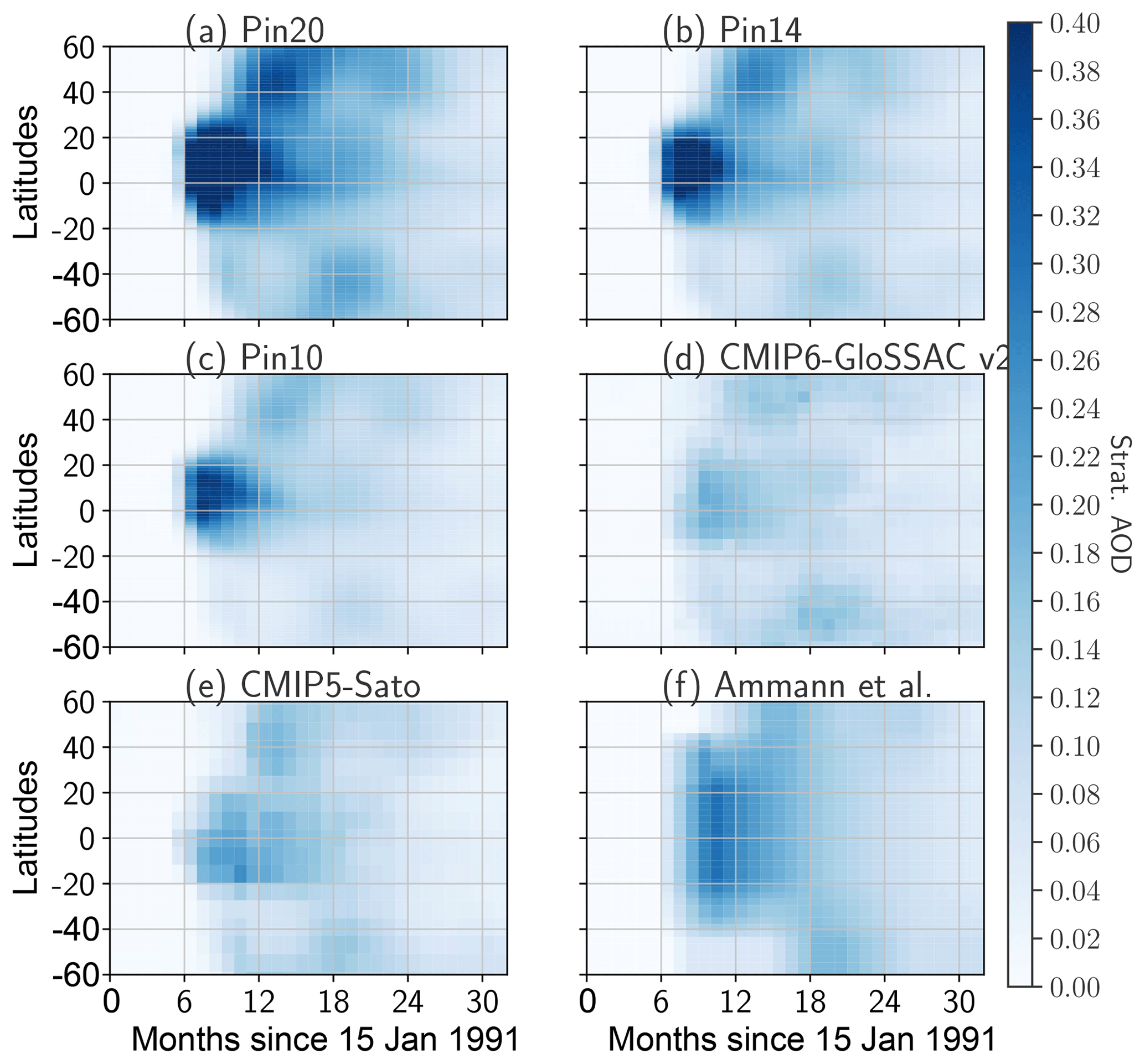
Figure 2 Ensemble mean stratospheric aerosol optical depth (sAOD) from simulations (a) Pin20, (b) Pin14, and (c) Pin10. Panels (d)–(f) show sAOD₅₅₀ from CMIP6-GloSSAC (Thomason et al., 2018), Sato (Sato et al., 1993), and Ammann (Ammann et al., 2003), respectively.

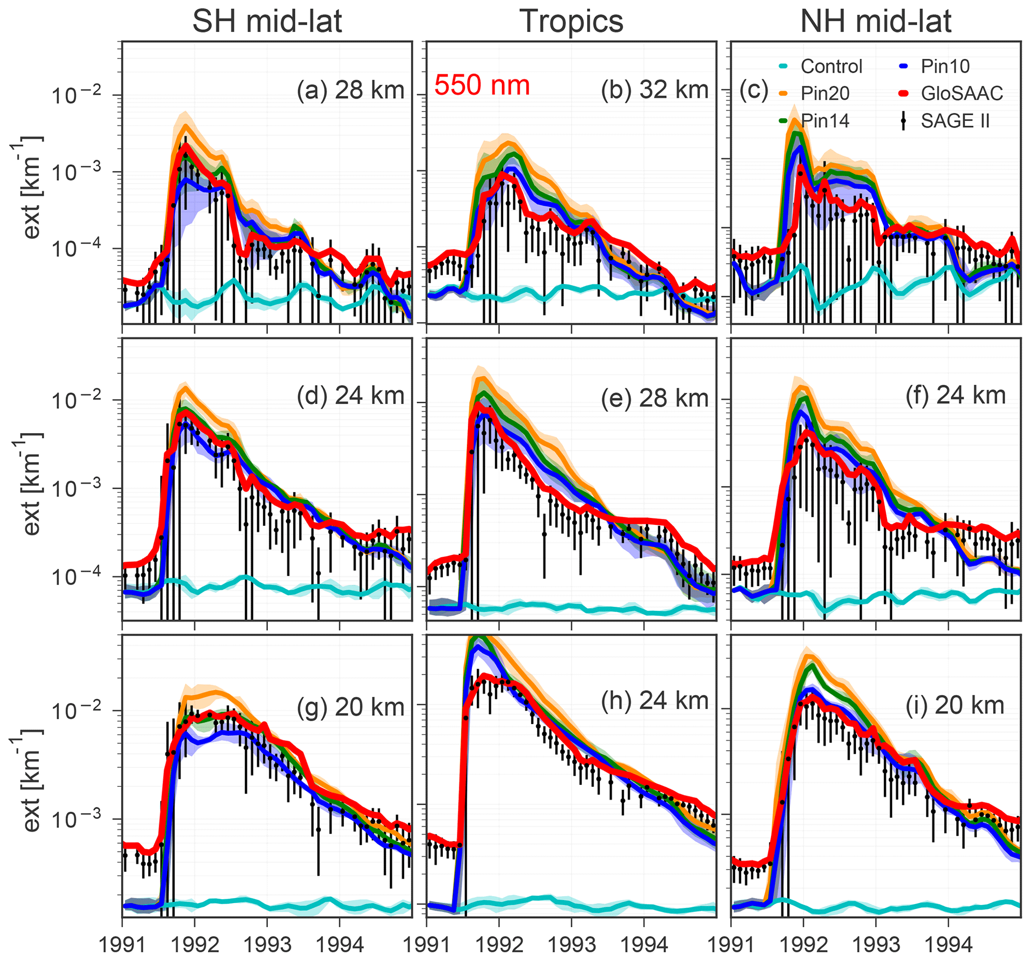
Figure 3 Ensemble mean extinctions (550 nm) from simulations Pin00 (aqua), Pin10 (blue), Pin14 (green), and Pin20 (orange). The shaded regions indicate the variability among ensemble members. Extinctions for SH mid-latitudes (35–60^∘ S, a, d, g), tropics (20^∘ S–20^∘ N, b, e, h), and NH mid-latitudes (35–60^∘ N, c, f, i) are shown. Mid-latitude extinctions are shown for 20, 24, and 28 km, whereas tropical profiles are shown for 24, 28, and 32 km. Monthly mean extinction from SAGE-II v7.2 measurements for a given latitude band are shown with black filled circles, and vertical lines indicate standard deviation from all the measurements for a given month. Gap-filled extinctions from the CMIP6-GloSSAC v2 dataset (Kovilakam et al., 2020) are shown with a red line.

As in the HIRS sulfur burden comparisons (Fig. 1), the Pin20 simulation, which best matches the satellite-observed SO₂ estimates, strongly over-predicts the sAOD in the tropics and Northern Hemisphere (NH) mid-latitudes, compared to all three reference datasets. However, whereas the lower emissions runs Pin10 and Pin14 both closely track the observed global column sulfur variation, run Pin10 has best agreement with all three reference datasets for mid-visible sAOD. For this run Pin14 is high-biased in the tropics and NH mid-latitudes. In the tropics, all three emission-magnitude ensembles are higher than the reference datasets.

Figure 2 illustrates the well-established global dispersion pattern for the Pinatubo aerosol cloud: initially confined to the tropical reservoir region, then dispersing to mid-latitudes, following the seasonal variation in the Brewer–Dobson circulation. The over-prediction in the tropics is a common feature among interactive stratospheric aerosol models. It is noticeable that this over-prediction is worst in the first 6–9 months after the eruption, which could indicate the source of the model's discrepancy. Whereas an overly non-dispersive tropical pipe in the model could be the cause, the timing is potentially more consistent with a missing loss pathway that is most effective in the initial months after the eruption. Co-emitted volcanic ash will also have been present within the tropical reservoir, as seen in the airborne lidar depolarisation measurements in the weeks after the eruption (Winker and Osborn, 1992) and remained present in the lowermost part of the mid-latitude aerosol cloud in both hemispheres (Young et al., 1992; Vaughan et al., 1994). The stratospheric aerosol optical depth (sAOD) high bias is consistent with the hypothesis that a substantial proportion of the emitted sulfur may have been removed from the stratosphere by accommodation onto the sedimenting ash. If this mechanism is causing such a vertical re-distribution within the tropical reservoir, it will increase the proportion of Pinatubo sulfur being removed into the troposphere via the rapid isentropic transport that occurred during the initial months in the lowermost stratosphere. Furthermore, sAOD is not a measure of sulfur, and the variations in sAOD will partly indicate changes in scattering efficiency that result from the gradient in effective radius that were apparent at the time, as discussed in this section.

The peak mid-visible sAOD from AVHRR is higher than the SAGE-II gap-filled satellite measurements (Long and Stowe, 1994). For example, as noted in Thomason et al. (2018), the peak mid-visible sAOD in the Advanced Very High Resolution Radiometer (AVHRR) dataset is around 0.4, compared to 0.22 in GloSSAC. However, other possible model biases cannot be ruled out. One consideration for these free-running simulations, even with each ensemble member initialised to approximate the period's QBO phase, is that nudging towards reanalysis meteorology would give more realistic representation of this initial phase of the plume dispersion (Sukhodolov et al., 2018). We chose to perform free-running simulations to allow the enhanced tropical upwelling resulting from increased LW aerosol-absorptive heating, consistent with the SO₂ emission, known to exert a strong influence on the subsequent simulated global dispersion (Young et al., 1994).

In contrast to the tropics and NH mid-latitudes, where run Pin10 agrees best with the reference datasets, run Pin14 compares best to the Southern Hemisphere (SH) sAOD₅₅₀ measurements in GloSSAC. This difference may be highlighting the requirement for a more accurate simulation of the QBO evolution, likely necessary to capture the Pinatubo cloud's transport to the SH mid-latitudes (e.g. Jones et al., 2016; Pitari et al., 2016). One thing to note is that our simulations do not include the source of volcanic aerosol from the August 1991 Cerro Hudson eruption in Chile. However, measurements from SAGE-II (Pitts and Thomason, 1993) and ground-based lidar (Barton et al., 1992) indicate that the Hudson aerosol cloud only reached to around 12 km, with the Pinatubo cloud by far the dominant contributor to SH mid-latitude sAOD. So, although we have not included the Hudson aerosol in our simulations, it is possible that a minor contributor from Cerro Hudson sAOD might reduce differences between Pin10 and CMIP6-GloSSAC V2 sAOD. Overall, the sAOD₅₅₀ comparisons confirm the findings from Fig. 1 that for UM-UKCA, consistent with other global microphysics models (Sheng et al., 2015a; Mills et al., 2016), Pinatubo aerosol properties are better simulated (acknowledging the discrepancy in the SH) with a 10 to 14 Tg range in volcanic SO₂ emission.

Although Fig. 2 suggests significant differences among the volcanic forcing datasets for the Pinatubo period, CMIP6-GloSSAC is the best-estimate dataset, with the 1991–1994 period in the Sato dataset mostly based on an earlier version of the SAGE-II data. The GloSSAC data have been compared extensively with lidar measurements (Antuña et al., 2002; Antuña, 2003) and these later combined for the gap-filled dataset (SPARC, 2006), with also improvements from the progression of the SAGE-II aerosol extinction retrieval algorithm (version 7).

For historical climate integrations in CMIP5, some models used the Sato forcing dataset, whilst others used Ammann and their differences affect interpretation of volcanic impacts among the models (Driscoll et al., 2012). For CMIP6, all models have harmonised to use the same forcing dataset, with a dedicated VolMIP analysis to compare the climate response in each model and with the CMIP6-GloSSAC Pinatubo forcing applied to the pre-industrial control (Zanchettin et al., 2016).

After comparing the total sulfur burden and sAOD, Fig. 3 shows UM-UKCA simulated mid-visible extinction at three different altitudes in the lower stratosphere, to evaluate the simulated vertical extent of the Pinatubo cloud through the global dispersion phase. For the tropics, extinction comparisons are shown at 24, 28, and 32 km, whereas for SH (35–60^∘ S) and NH (35–60^∘ N) mid-latitudes the chosen levels are 20, 24, and 28 km to account for the higher tropical tropopause. Simulated extinctions are compared with raw SAGE v7.0 data (Damadeo et al., 2013) as well as the gap-filled extinction from CMIP6-GloSSAC at 525 nm. As discussed previously, extinctions from Pin14 (and to some extent Pin10) show much better agreement with observational data for all three latitude bands. Most importantly, model extinction remains close or slightly lower in the mid-latitude compared to SAGE-II extinction even after 4 years, suggesting that the sharp decay in sulfur burden observed by Baran and Foot (1994) may be unrealistic. Interestingly, in the SH mid-latitudes, extinction from Pin14 shows much better agreement with SAGE-II extinctions at 20 and 24 km. This again confirms biases discussed in Fig. 2 that could be attributed to the weaker lower-stratospheric transport in the SH mid-latitudes, and the Cerro Hudson eruption must have contributed only slightly to the observed sAOD. At 1020 nm, agreement is even better (See Fig. S3). Also as observed in Figs. 1 and 2, extinction differences between runs Pin10, Pin14, and Pin20 are largest for the first few months after the eruption but extinction lines almost overlap within ensemble variance from each eruption. This again confirms that as a greater amount of volcanic SO₂ is injected into the stratosphere, the cloud evolves to a larger average particle size, leading to faster sedimentation.

A key feature seen in Fig. 3 that is not captured well in any Pinatubo simulation is the plateau in the SAGE-II (and GloSSAC) tropical peak extinction. For example, at 24 km (where the instrument saturation effect should be minimal), after reaching peak values within first 3 months, extinction values remain approximately constant for at least 6 months. At 20 km, this plateau in extinction in the tropics is visible for almost 12 months in the CMIP6-GloSSAC data (not shown). Similar features are visible at 1020 nm extinction (Fig. S3). If indeed these plateau features in the SAGE-II data are realistic, then they would need to have been caused by the sustained tropical upwelling (via upward branch of Brewer–Dobson circulation, combined with aerosol-induced heating), being offset by sedimentation of the particles that would have grown via condensation and coagulation. These plateau structures in extinctions are not apparent in the mid-latitudes of either hemisphere, with a clear seasonal cycle occurring due to preferential wintertime circulation (e.g. Dhomse et al., 2006, 2008) that is visible in both model and SAGE-II data.

A notable discrepancy is that modelled extinction is low-biased (by up to 50 %) during pre-eruption months. This could be associated with low background sulfur burden in our model or slightly elevated stratospheric aerosol due to small volcanic eruptions (such as Mt Redoubt 1989/90, Kelud,1990) that are not included in our simulations. Another explanation could be due to the fact that the model does not resolve the uptake of organics into the particle phase. Observations (Murphy et al., 2007) and modelling studies (Yu et al., 2016) have shown that organic-sulfate particles (Murphy et al., 2014) are the dominant aerosol type in the tropical and mid-latitude upper troposphere and lower stratosphere, and the omission of this interaction might have introduced systematic low bias during background periods.

Next we evaluate the meridional, vertical, and temporal variations in effective radius (R_eff) in the Pinatubo UM-UKCA datasets. The particle size variations in these interactive simulations of the Pinatubo cloud reflect the chemical and microphysical processes resolved by the chemistry–aerosol module, in association with the stratospheric circulation and dynamics occurring in the general circulation model. We analyse these model-predicted size variations alongside those in the benchmark observation-based R_eff dataset from CMIP6-GloSSAC, which applies the 3λ size retrieval from the 453, 525, and 1020 nm aerosol extinction measurements from SAGE-II (Thomason et al., 1997a, 2018).

Figure 4 shows zonal mean R_eff at 25 km, within the altitude range of the volcanic SO₂ injection, and at 20 km, underneath the main volcanic cloud. Results are shown from three-member means from the 10, 14, and 20 Tg SO₂ emission runs (Pin10, Pin14, and Pin20). For comparability with the equivalent figure from Dhomse et al. (2014), the Supplement (Fig. S6) shows the updated comparison to the Bauman et al. (2003) R_eff dataset. Overall, the model captures the general spatio-temporal progression in the R_eff variations seen in the GloSSAC dataset. However, whereas the 10 and 14 Tg simulations agree best with the HIRS-2 sulfur burden (Fig. 1) and the GloSSAC sAOD and extinction (Figs. 2 and 3), the magnitude of the R_eff enhancement is best captured in the 20 Tg run (Pin20). The comparisons suggest the low bias in simulated R_eff seen in the previous UM-UKCA Pinatubo study (Dhomse et al., 2014) is still present here. However, this low bias in particle size/growth may simply be reflecting the required downward adjustment of the Pinatubo SO₂ emission, as a larger R_eff enhancement in the 20 Tg simulation is clearly apparent. It is possible that the two-moment modal aerosol dynamics in GLOMAP-mode may affect its predicted R_eff enhancement. However, the model requirement for reduced SO₂ emission is attributed to be likely due to a missing, or poorly resolved, model loss pathway, such as accommodation onto co-emitted volcanic ash. The sustained presence of ash within the Pinatubo cloud (e.g. Winker and Osborn, 1992) will likely have altered particle size and growth rates in the initial months after the eruption.

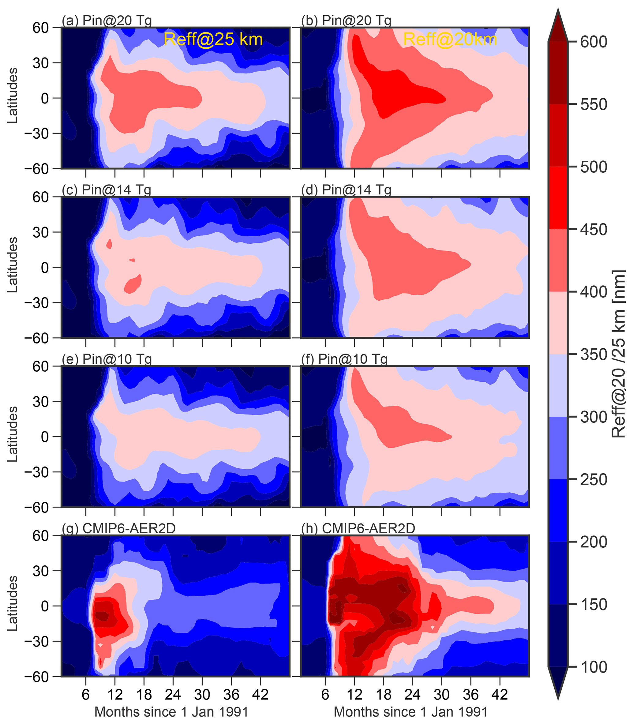
Figure 4 Modelled effective radii (R_eff, in µm) from (a, b) simulation Pin20, (c, d) simulation Pin14, (e, f) simulation Pin10, and (g, h) CMIP6-GloSSAC V2 at (a, c, e, g) 25 km, and (b, d, f, h) 20 km.

In the tropics, where R_eff increases are largest, the time series of R_eff is noticeably different in the core of the tropical reservoir (10^∘ S to 10^∘ N) to that in the edge regions (10–20^∘ N and 10–20^∘ S), at both 20 and 25 km. The R_eff increases in these edge regions occur when tropics to mid-latitude transport is strongest, in phase with the seasonal cycle of the Brewer–Dobson circulation, which tends to transport air towards the winter pole (Butchart, 2014). The R_eff increases are due primarily to particle growth from coagulation and condensation, and the simulations also illustrate how the simulated Pinatubo cloud comprises much smaller particles at 25 km than at 20 km. The 25 km level is in the central part of the Pinatubo cloud, particles there being younger (and smaller) because the oxidation of the emitted volcanic SO₂ that occurs at that level triggers extensive new particle formation in the initial months after the eruption (e.g. Dhomse et al., 2014). By contrast, at the 20 km level particles will almost exclusively have sedimented from the main cloud and therefore be larger. There is a slow but sustained increase in average particle size in the equatorial core of the tropical Pinatubo cloud, with the 20 km level reaching peak R_eff values only during mid-1992, in contrast to the peak sulfur burden and sAOD₅₅₀ which have already peaked at this time, being in decay phase since the start of 1992 (see Figs. 1 and 2).

Whereas the simulated peak R_eff enhancement occurs by mid-1992 in the tropics, the peak R_eff in NH mid-latitudes occurs at the time of peak meridional transport, the R_eff variation there reflecting the seasonal cycle of the Brewer–Dobson circulation, as also seen in the tropical reservoir edge region. The different timing of the volcanic R_eff enhancement in the tropics and mid-latitudes is important when interpreting or interpolating the in situ measurement record from the post-Pinatubo OPC soundings from Laramie (Deshler, 2003). Russell et al. (1996) show that the R_eff values derived from Mauna Loa ground-based remote sensing are substantially larger than those from the dust-sonde measurements at Laramie. The interactive Pinatubo simulations here confirm this expected meridional gradient in effective radius, with the chemical, dynamical, and microphysical processes also causing a vertical gradient in the tropical to mid-latitude R_eff ratio. The current ISA-MIP activity (Timmreck et al., 2018) brings a potential opportunity to identify a consensus among interactive stratospheric aerosol models for the expected broad-scale spatio-temporal variations in uncertain volcanic aerosol metrics such as effective radius.

An important aspect of volcanically enhanced stratospheric aerosol is that they provide surface area for catalytic ozone loss (e.g. Cadle et al., 1975; Hofmann and Solomon, 1989). A comparison of stratospheric sulfate area density for 3 different months (December 1991, June 1992 and December 1992) is shown in Fig. 5. SAD derived using observational data (Arfeuille et al., 2014), also known as 3λ SAD, is also shown. Again, Pin20 SAD shows a high bias, whereas Pin10 SAD seems to show good agreement with 3λ data. Our simulations do not include the SO₂ injection from the August 1991 Cerro Hudson eruption (Chile), yet the model captures the volcanic SAD enhancement in the SH mid-latitude stratosphere very well. The model does not capture the enhanced SAD signal at 10–12 km in the SH in December 1991; the altitude of that feature in the 3λ dataset is consistent with lidar measurements of the Hudson aerosol cloud from Aspendale, Australia (Barton et al., 1992). The most critical differences are that 3λ SAD are confined in the lowermost stratosphere. A deeper cloud of enhanced SAD, with steeper low–high-latitude SAD gradients, is visible in all the model simulations. As seen in Fig. 3, by June 1992 tropical SAD from runs Pin10 and Pin14 are low-biased, indicating lower aerosol in the tropical pipe which could be either due to faster transport to the high latitudes (weaker sub-tropical barrier in the middle stratosphere) and/or quicker coagulation causing faster sedimentation.

Figure 5 Zonal mean monthly mean surface area density (SAD, µm² cm⁻³) for December 1991, June 1992, and December 1992 from ensemble mean simulations (top row) Pin20, (second row) Pin14, and (third row) Pin10, The bottom row shows observation-based SAD estimates from Arfeuille et al. (2014).

Figure 6 shows the time series of observed SW and LW radiative near-global mean flux anomalies (60^∘ S–60^∘ N), with respect to a 1985 to 1989 (pre-Pinatubo) baseline. The ERBE data (black symbols) are from Edition 3 Revision 1, non-scanner, wide field-of-view observations (Wielicki et al., 2002; Wong et al., 2006). Coloured lines indicate ensemble mean forcing anomalies from three Pinatubo SO₂ emission scenarios. The Pin10 simulation generates a peak solar dimming of 4 W m⁻², matching well both the timing and magnitude of the peak in the ERBE SW anomaly time series. It is notable that if the ERBE SW anomaly is calculated relative to the 1995–1997 baseline, we estimate a peak solar dimming of 5.5 W m⁻² (not shown), which then compares best with the Pinatubo SW forcing from Pin14. Consistent with the sulfur burden, sAOD550 and mid-visible extinction comparisons (Figs. 1, 2 and 3), the Pin20 simulation also over-predicts the magnitude of the Pinatubo forcing compared to the ERBE anomaly. It is important to note here that the model Pinatubo forcings are not only from the volcanic aerosol cloud but also include any effects from the simulated post-Pinatubo changes in other climate forcers (e.g. stratospheric ozone and water vapour). As expected run Pin20 shows largest anomalies in both SW and LW radiation and distinct differences between Pin10, Pin14, and Pin20 are visible until the end of 1992. For this 10 to 20 Tg emission range, we find the global-mean SW forcing scales approximately linearly with increasing SO₂ emission amount, the 40 % increase from 10 to 14 Tg and 43 % increase from 14 to 20 Tg causing the Pinatubo SW forcing to be stronger by 34 % (4.1 to 5.5 W m⁻²) and 36 % (5.5 to 7.5 W m⁻²), respectively.

Figure 6 Near-global (60^∘ S–60^∘ N) longwave (LW) and shortwave (SW) heating anomalies (W m⁻²) from the ensemble mean of simulations Pin20(blue), Pin14 (green), and Pin10 (orange). Estimated anomalies from the Earth Radiation Budget Experiment (ERBE) satellite data are shown with black stars.

In contrast to the SW forcings, the magnitude of the anomaly in the peak LW forcing is best matched in the Pin20 simulation, although the Pin14 simulation also agrees quite well with the ERBE anomaly time series. Whereas the Pinatubo SW forcing closely follows the mid-visible aerosol changes, the LW forcing is more complex to interpret. Simulated LW aerosol absorption is not studied in this paper and almost certainly has a different temporal variation than the 550 and 1020 nm extinction variations analysed here. Also, the model LW forcing also includes effects from the dynamical changes in stratospheric water vapour which partially offset the SW dimming (e.g. Joshi and Shine, 2003) adding to the LW aerosol effect. Our simulations do not include co-emission of water vapour, which might have influenced stratospheric chemistry (e.g. LeGrande et al., 2016) and altered observed Pinatubo forcing. Another possible explanation for this discrepancy might be a poorly sampled signal in LW radiation alongside ERBE temporal coverage (36 d vs. 72 d). Again, as in the sulfur burden and extinction comparisons, after January 1992 observed SW anomalies seem to decay at a faster rate compared to all the model simulations.

Another important volcanic impact is the aerosol-induced heating in the lower stratosphere as large particles absorb outgoing LW radiation. Since the ERA-Interim analysis assimilates radiosonde observations from a large number of sites in the tropics, we can compare the temperature anomaly to the model predictions, as a further independent test. However, exact quantification of this mechanism is somewhat complicated as the ERA-Interim stratospheric temperature anomalies also include influence from other chemical and dynamical changes such as variations in ozone and water vapour as well as QBO and El Niño–Southern Oscillation (ENSO)-related changes in tropical upwelling (e.g. Angell, 1997b; Randel et al., 2009). We can assume the 5-year anomalies will remove the effects of some of the short-term processes. Figure 7 shows ERA-Interim temperature anomalies compared to the model's volcanic warming, i.e. the temperature difference between the sensitivity (Pin10, Pin14, and Pin20) and control (Pin00) simulations. Although we compare the simulated Pinatubo warming (temperature difference) to ERA-Interim temperature anomalies, it is only intended to provide an approximate observational constraint for the magnitude of the effect and the altitude at which it reaches a maximum. The Pin10 simulation best captures the magnitude of the ERA-Interim post-Pinatubo tropical temperature anomalies, and the model simulations and reanalysis both show maximum warming occurred in the 30 to 50 hPa range around 3–4 months after the eruption. The model predicts that the Pinatubo aerosol cloud continued to cause a substantial warming (>2 K) throughout 1992, which propagates downwards as found in ERA-Interim temperature anomalies.

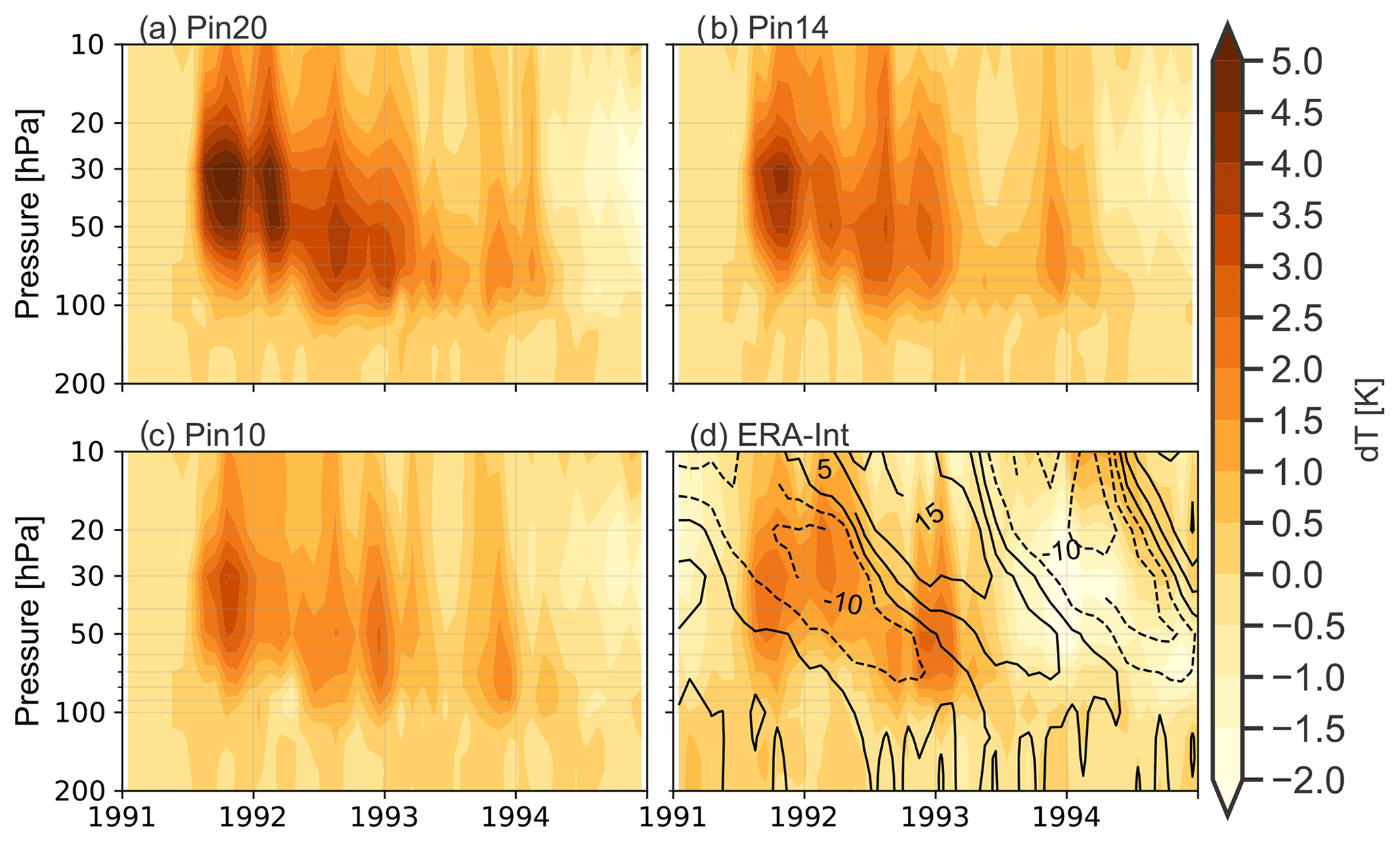
Figure 7 (a–c) Ensemble mean aerosol-induced heating (K) in the tropical (20^∘ S–20^∘ N) stratosphere, calculated by subtracting temperature fields from a control simulation for simulations Pin20, Pin14, and Pin10. (d) Tropical temperature (shaded) and zonal wind (contour) anomalies from ERA-Interim reanalysis data (for 1991–1995 time period). Contour intervals for wind anomalies are 4 m s⁻¹ and negative anomalies are shown with dashed lines.

4.2 El Chichón aerosol cloud

Whereas Pinatubo is often the main case study to evaluate interactive stratospheric aerosol models, El Chichón provides a different test as its volcanic aerosol cloud dispersed almost exclusively to the NH. We therefore seek to understand whether the biases seen for Pinatubo (over-predicted tropical sAOD and discrepancy between literature estimates of SO₂ emission and the peak global aerosol loading) are also seen for this alternative major eruption case.

Both El Chichón and Pinatubo eruptions occurred in the modern satellite era; however, there are far fewer datasets available for the evaluation of El Chichón aerosol properties as it occurred in the important gap period between SAGE-I and SAGE-II (see Thomason et al., 2018). As there are quite extensive observational data records for the El Chichón volcanic aerosol clouds (e.g. McCormick and Swissler, 1983; Hofmann and Rosen, 1983a), combining these with satellite datasets would greatly reduce large uncertainties concerning the evolution of the El Chichón aerosol cloud (e.g. Sato et al., 1993; SPARC, 2006).

Here, our analysis focuses primarily on comparing simulated mid-visible sAOD at 550 nm (sAOD₅₅₀) to the CMIP6 and Sato datasets. We also test the simulated vertical extent of the El Chichón cloud, comparing extinction at 20 and 25 km to the SAGE-II (and GloSSAC) data record, and compare the model simulated warming in the tropical lower stratosphere to temperature anomalies in the ERA-Interim reanalyses.

Figure 8 compares ensemble mean sAOD₅₅₀ from Elc05, Elc07, Elc10, and three observation-based datasets. Overall, there are significant differences between simulated sAOD₅₅₀ and the observations. The CMIP6-GloSSAC dataset enacts the strongest solar dimming in NH mid-latitudes (peak sAOD₅₅₀ of 0.14), the tropical reservoir never exceeding an sAOD of 0.08, whereas the Sato and Ammann datasets enact the highest sAOD₅₅₀ in the tropics. The model simulations also find the highest solar dimming occurred in the tropical reservoir, with the mean of the 5 Tg simulations predicting a maximum sAOD₅₅₀ of about 0.28. With the QBO in the westerly phase, and timing of the eruption (4 April), the Brewer–Dobson circulation readily exported a large fraction of the plume to the NH, but the meridional gradient in the solar dimming is an important uncertainty to address in future research

Figure 8 Same as Fig. 2 but for El Chichón simulations (a) Elc10, (b) Elc07, and (c) Elc05.

In the model the depth of the tropical volcanic aerosol reservoir that forms is closely linked to the altitude of the volcanic SO₂ emission. We aligned our experiments with the ISA-MIP HErSEA experiment design (Timmreck et al., 2018), specifying a 24–27 km injection height based on the airborne lidar measurement surveys of the tropical stratosphere that provide the main constraint for the gap-filled dataset (see Fig. 4.34 in SPARC, 2006). Balloon measurements from southern Texas and Laramie (Hofmann and Rosen, 1983b) and the constraints from the airborne lidar survey flights in July, September, and October (McCormick and Swissler, 1983) together show that a large part of the plume was transported early to NH mid–high latitudes via the middle branch of the Brewer–Dobson circulation to around 25 km, with lower altitudes of the cloud remaining confined to the tropical reservoir. The evolution of the cloud is complex and strongly influenced by several factors, including the rate of SO₂ conversion to aerosol and the depletion of oxidants, the tropical upwelling of the Brewer–Dobson circulation, sedimentation of the ash and sulfuric acid droplets (and their interactions), and the downward-propagating QBO. The multiple interacting processes within the tropical reservoir makes analysis of this early phase dispersion a complex problem, yet their combined net effects determines the subsequent transport of the aerosol to mid-latitudes and the resulting radiative forcing.

Due to significant differences observed in Fig. 8, even with limited SAGE-II observations, simulated extinctions are compared in Fig. 9. Simulated extinctions for all three SO₂ emission scenarios show an excellent agreement with SAGE-II from October 1984 onwards. Similarly, extinction at 1020 nm also shows very good agreement with SAGE-II data that are shown in Fig. S4. A sudden jump in the CMIP6-GloSSAC data at the start of the SAGE-II period is evident as are other unexplained sudden increases in extinction earlier in the CMIP6 dataset, e.g. in the SH at 24 km. On the other hand, the somewhat elevated SAGE-II extinction in the NH mid-latitudes compared to model extinctions highlights a possible model discrepancy due to the injection altitude leading to faster removal of the aerosol particles. GloSSAC extinction in the SH mid-latitude shows very little seasonal variation, and the sudden changes seen at both 20 and 24 km are surprising and difficult to reconcile with expected variation. They could potentially be artefacts from the interpolation procedure. Overall, Fig. 9 clearly suggests potential areas where combining with models may help improve the CMIP6-GloSSAC (and other) datasets, highlighting the need for combining observational data with El Chichón-related model simulations to better represent the consistency and variations within the El Chichón surface cooling included in climate models.

Figure 9 Same as Fig. 3 but for El Chichón simulations (a) Elc05, (b) Elc07 and (c) Elc10.

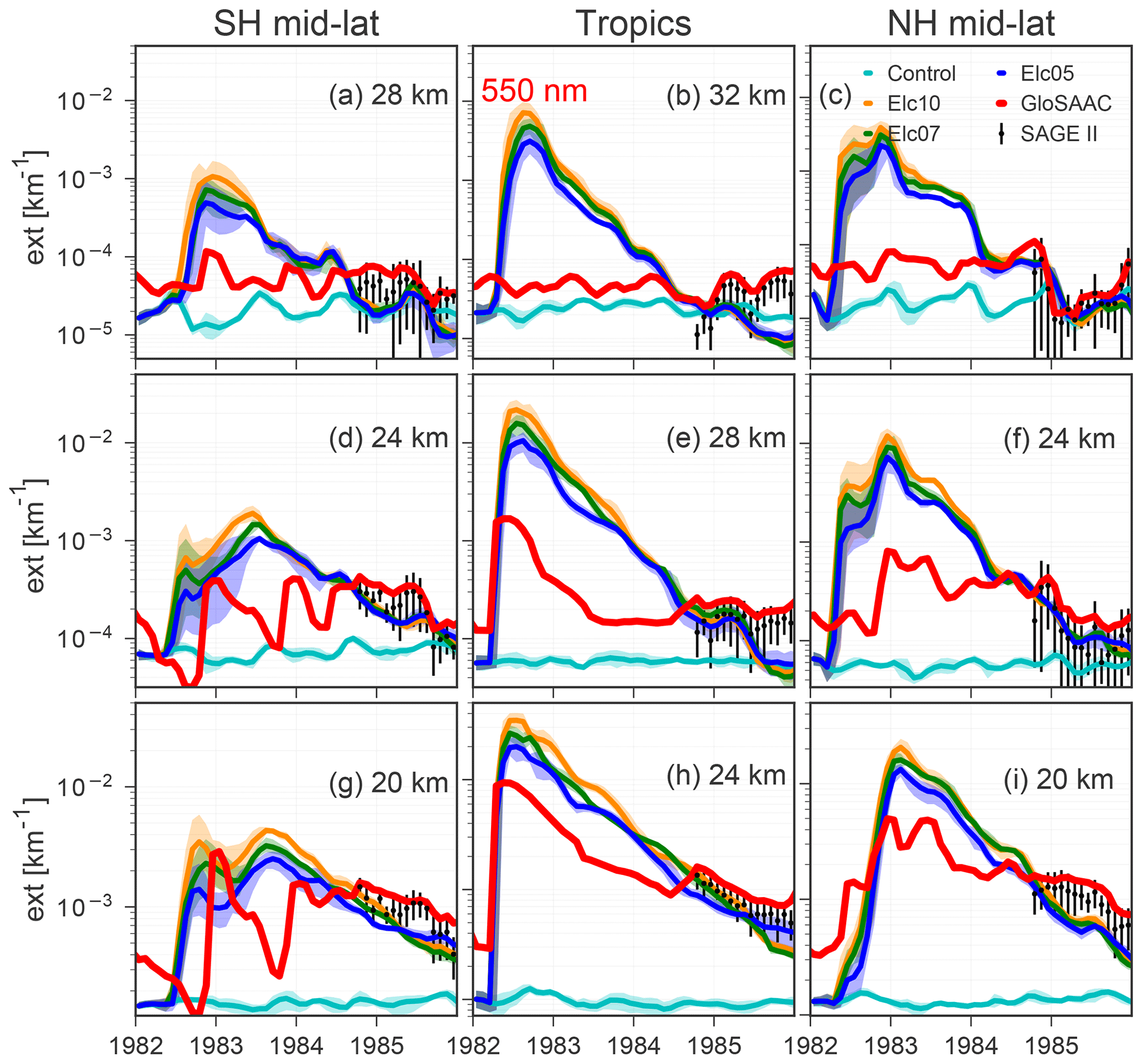
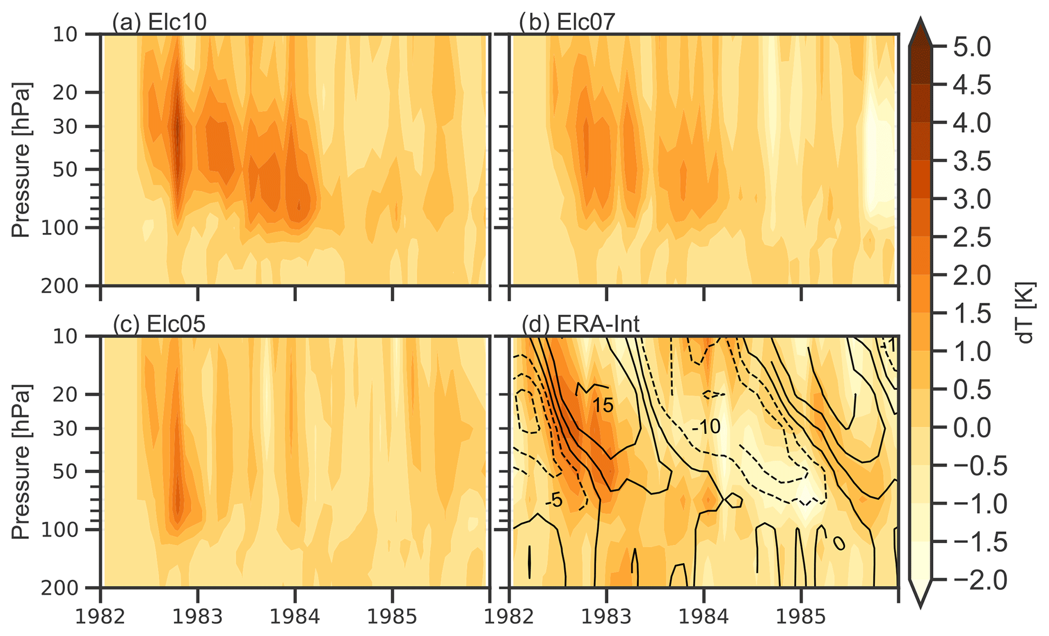
Figure 10 shows the tropical warming of the stratosphere predicted by the model, comparing it again to the ERA-Interim temperature anomaly (compared to the mean for 1982–1986). As in the Pinatubo case (Fig. 7), the speed of downward propagation of these anomalies seems to be well captured by all the simulations. Peak warming of about 3 K observed in ERA-Interim between 30 and 50 hPa seems to be well reproduced in Elc07. Warm anomalies (up to 1 K) visible in ERA-Interim data between 10 and 20 hPa suggest the downward-propagating westerly QBO contributed to up to 1 K warming; hence the simulated warming will be about 1 K less than the ERA-Interim anomalies. Overall, Elc05 seems to reproduce the El Chichón-related warming more realistically, but the slight warming persisting near 70 hPa until March 1983 is absent in this simulation. Again this suggests that for UM-UKCA, 5 and 7 Tg are reasonable lower and upper limits of SO₂ injection required to simulate observed lower-stratospheric warming.

Figure 10 Same as Fig. 7 but for El Chichón simulations (a) Elc10, (b) Elc07, and (c) Elc05.

4.3 Mt Agung aerosol cloud

The El Chichón and Pinatubo eruptions occurred when satellite instruments were monitoring the stratospheric aerosol layer, and the global dispersion of their volcanic aerosol clouds is relatively well characterised. For the Agung period our knowledge of the global dispersion is less certain and primarily based on the synthesis of surface radiation measurements from Dyer and Hicks (1968). These measurements show the Agung cloud dispersed mainly to the SH, although aerosol measurements from 10 balloon-borne particle counter soundings from Minneapolis in 1963–1965 (Rosen, 1964, 1968) and 66 ground-based lidar profiles from Lexington, Massachusetts, in 1964 and 1965 (Grams and Fiocco, 1967) show substantial enhancement in the NH as well. For this period, the Sato forcing dataset enacts solar dimming following the ground-based solar radiation measurements discussed in Dyer and Hicks (1968), whereas the CMIP6-AER2D dataset is based on a partially rescaled 2-D interactive stratospheric aerosol model simulation of the Agung aerosol cloud.

To address these limitations, the SPARC (Stratosphere-Troposphere Process and their Role in Climate Project) project entitled SSiRC (Stratospheric Sulfur and its Role in Climate) initiated a stratospheric aerosol data rescue project (see http://www.sparc-ssirc.org/data/datarescueactivity.html, last access: 15 June 2020). Its primary aim is to gather, and in some cases recalibrate, stratospheric aerosol measurements from major volcanic periods, to provide new constraints for stratospheric aerosol models. For example, ship-borne lidar measurements of the tropical volcanic aerosol reservoir during the SAGE-II saturation period after Pinatubo have recently been recovered (Antuña Marrero et al., 2020b). One part of this study contributes to this SSiRC activity, with the recovery of the 1964–1965 lidar measurements made by Grams and Fiocco (1967), the observations then used to evaluate the vertical extent of the Agung aerosol cloud.

Figure 11 compares sAOD₅₅₀ from model simulations with CMIP6-AER2D, Sato, and Ammann data. Both CMIP6 and Sato datasets suggest that the tropical volcanic aerosol cloud dispersed rapidly, and almost exclusively, to the SH which is also consistent with our understanding of QBO-dependent meridional transport (Thomas et al., 2009). During the westerly QBO phase, the volcanic plume is quickly transported towards the winter hemisphere, whereas during the easterly phase, the tropics-to-high-latitude transport is slower; hence some part of the plume is available for the wintertime transport into the opposite hemisphere. In contrast, the Ammann dataset has a significant portion of the cloud transport to the NH, the dispersion parameterisation considering only seasonal changes in stratospheric circulation. Differences from the Amman dataset therefore illustrate the modulation of meridional transport caused by the QBO, which in the Agung case increases the export from low latitudes to mid-latitudes.

Figure 11 Same as Fig. 2 but for Mt Agung simulations (a) Agu12, (b) Agu09, and (c) Agu06.

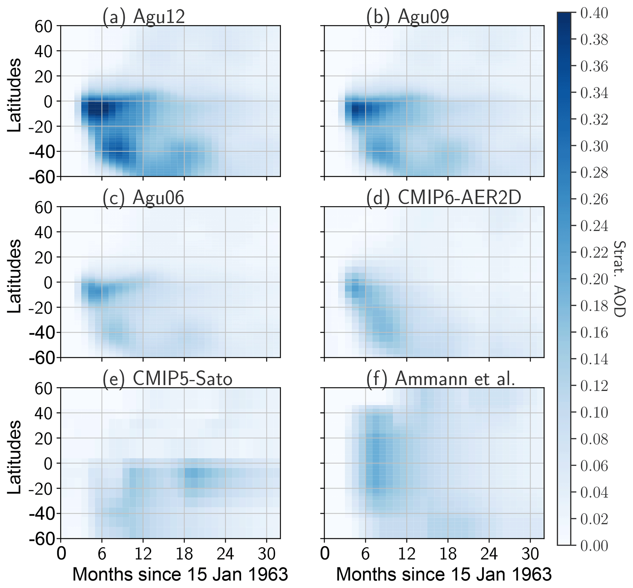
Figure 11 also shows that for the post-Agung period there are very large differences in the sAOD₅₅₀ between the CMIP6-AER2D and Sato datasets. Hence there will have been substantially different Agung surface cooling within historical climate integrations for the two most recent CMIP assessments. Overall, the CMIP6 dataset generates much stronger peak sAOD₅₅₀ than the Sato dataset, with a peak of around 0.2 in the tropics, just a few months after the eruption. The Sato dataset shows a peak value of about 0.12, which suddenly drops below 0.05 within couple of months. Thereafter, there is a steady build-up with a local peak in sAOD₅₅₀ occurring in November 1963, 8 months after the eruption. The Sato dataset then enacts a much stronger second peak in tropical sAOD₅₅₀ in August–September 1964 that must be based on measurements from Kenya and the Congo (Dyer and Hicks, 1968). By contrast, CMIP6-AER2D predicts the Agung cloud dispersed rapidly to the SH with the tropical reservoir reducing to sAOD₅₅₀ of less than 0.05 at that time. Our simulations predict the Agung aerosol dispersed to the SH with similar timing to the CMIP6 dataset but with a larger proportion remaining in the tropical reservoir. Similar to the CMIP6 datasets, our simulations also predict a secondary sAOD₅₅₀ peak in SH mid-latitudes near 40^∘ S. Although a similar pattern is produced in almost all simulations, sAOD₅₅₀ from Agu06 seems to be in much better agreement with CMIP6 data.

These comparisons highlight that there is still substantial uncertainty about the global dispersion of the Agung cloud. However, there are extensive sets of stratospheric aerosol measurements carried out during this period (see http://www.sparc-ssirc.org/data/datarescueactivity.html, last access: 15 June 2020). Hence, there is potential to reduce this uncertainty combining these observations also with interactive stratospheric model simulations (Timmreck et al., 2018). Dyer and Hicks (1968) discuss the transport pathways for the volcanic aerosol, in relation to seasonal export from the tropical reservoir. Stothers (2001) analysed a range of measurements to derive the turbidity of the Agung cloud, but they chose to omit the surface radiation measurements from the Kenya and Congo sites in their analysis, attributing a lower accuracy to those observations. It is notable that the high sAOD measurements were made during the dry season, when other sources of aerosol could potentially have caused additional solar dimming. In terms of modelling, Niemeier et al. (2019) discussed possible implications of two separate Agung eruptions in 1963. They performed two model simulations: one with a single eruption and one with two separate eruptions on 17 March and 16 May with 4.7 and 2.3 Tg SO₂ injection, respectively. They found significant differences between simulated aerosol properties and available evaluation datasets. They suggested that two separate eruptions are necessary to simulate the climatic impact. However, due to limited observational data they could not validate their model results extensively. They also discussed that simulated sAOD₅₅₀ differences with respect to evaluation data are larger than the differences between their two simulations. Pitari et al. (2016) also present global mean sAOD₅₅₀ changes after the Agung eruption with a single eruption (12 Tg on 16 May 1963), but they did not show the latitudinal extent of the Agung volcanic cloud dispersion.

Figure 12 compares simulated and CMIP6-AER2D extinctions at 550 nm at 16, 20, and 24 km. As in previous figures the tropical comparison is shifted upwards by 4 km. Overall, modelled and CMIP6 extinctions show an almost identical decay rate. At 16 km, nearly all the model simulations show a high bias compared to CMIP6 data and model extinction. On the other hand, at 20 km, tropical CMIP6 extinction seems to peak a bit later and there is better agreement in the mid-latitude extinction in both hemispheres. The UM-UKCA extinctions reflect the primary influence of the QBO on the sub-tropical barrier (edge of the tropical reservoir), as well as the fact that meridional transport occurs preferentially towards the winter hemisphere. The differences between our model and CMIP6 extinction must be primarily due to injection altitude and the simplified stratospheric dynamics in the 2D model used to construct CMIP6 data.

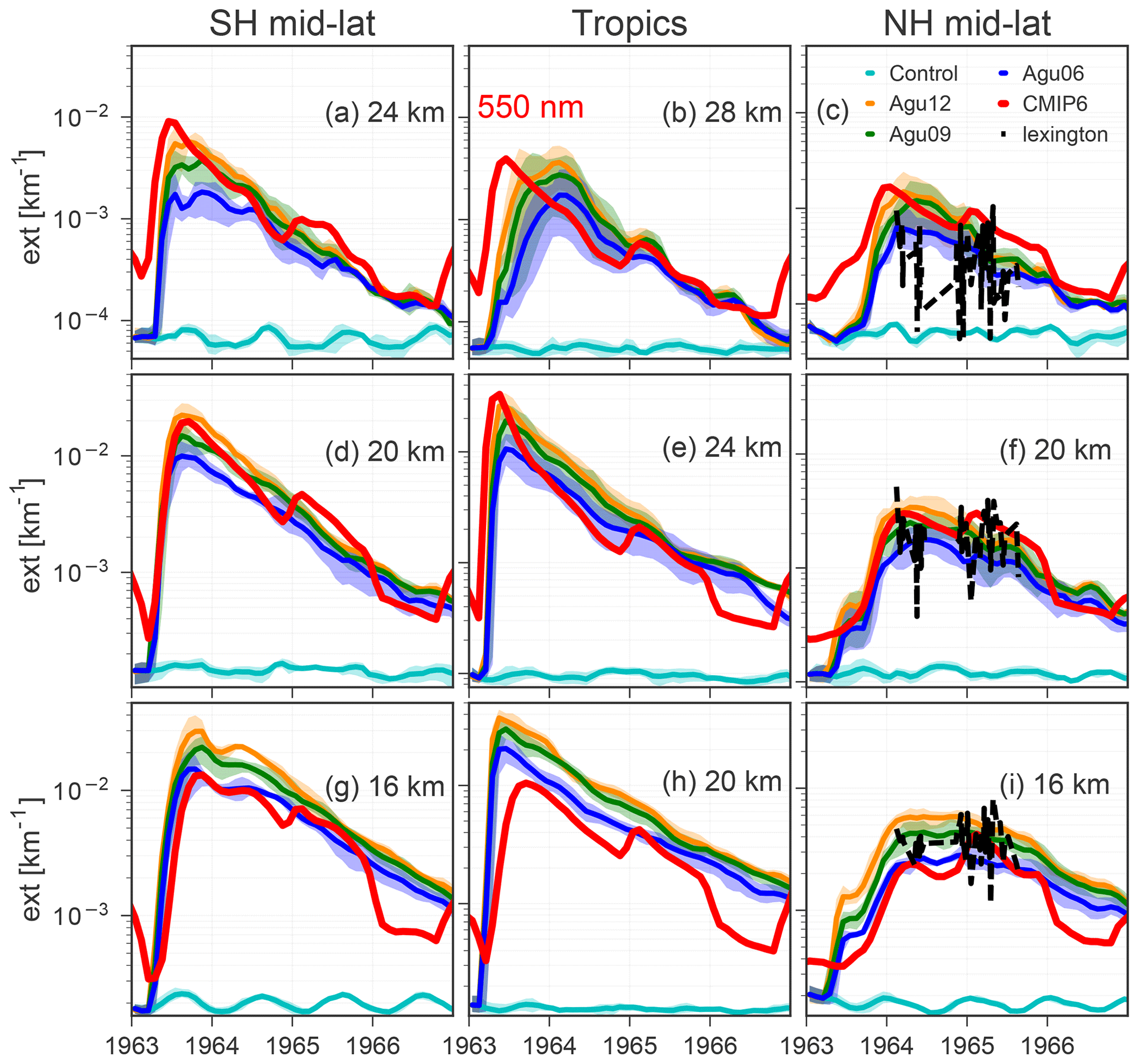
Figure 12 Same as Fig. 3 but for Mt Agung simulations Agu06, Agu09, and Agu12. Mid-visible aerosol extinctions are shown at 16, 20, and 24 km for mid-latitudes and at 20, 24, and 28 km for the tropics. Also shown are aerosol extinctions from the CMIP6-AER2D dataset (Arfeuille et al., 2014) and from lidar measurements at a NH mid-latitude site (Lexington, Massachusetts, USA) (Grams and Fiocco, 1967).

Figure 12 also shows the extinction from the 1964–1965 ground-based lidar at Lexington, Massachusetts (42^∘44^′ N, 71^∘15^′ W) as presented in Grams and Fiocco (1967). The method used to convert lidar backscatter to extinction is described in the Supplement. Although the lidar data show large variability, these single location measurements still provide insight into the transport of the Agung aerosol cloud in the NH. At 16 km, Agu09 seem to show best agreement with lidar data, although by spring 1965, simulated extinctions are lower than the lidar data, which could potentially indicate fresh volcanic aerosol from 1964 eruptions in Iceland and Alaska (see Antuña Marrero et al., 2020c). A similar pattern is observed at 20 km. Somewhat larger lidar extinction in spring 1965 compared to model simulations might be due to either weak transport from the tropics to the NH mid-latitudes (more transport to the SH) in the model, or aerosol removal is too fast in our simulations. Extinctions at 24 km are shown in Fig. S5 and again confirm good agreement between lidar and Agu09. Overall, the extinction comparison with the Lexington lidar data suggests that transport of the Agung volcanic cloud and its vertical extent into the NH mid-latitudes is well represented in Agu09.

Finally, we compare tropical warming in Fig. 13. As ERA-Interim reanalyses starts in 1979, we calculate observationally based anomalies from ERA-40 data. Bearing in mind that almost all the reanalysis datasets have significant inhomogeneities in the pre-satellite era, observation-based warming estimates should be treated carefully. However, as expected ERA-40 data show almost 1 K warming in the middle stratosphere before the eruption indicating downward propagation of warmer anomalies associated with the westerly QBO. Using radiosonde data, Free and Lanzante (2009) attributed around 1.5 K warming to the Mt Agung volcanic aerosol near 50 hPa, which is somewhat consistent with ERA-40 (after removing 1 K warming due to the westerly QBO). However, almost all of the simulations show 1–2 K more warming compared to ERA-40 data as modelled temperature differences do not include QBO-related anomalies.

Figure 13 Same as Fig. 7 but for Agung simulations (a) Agu12, (b) Agu09, and (c) Agu06 and for (d) temperature anomalies calculated using ERA-40 reanalysis data.

5 Conclusions

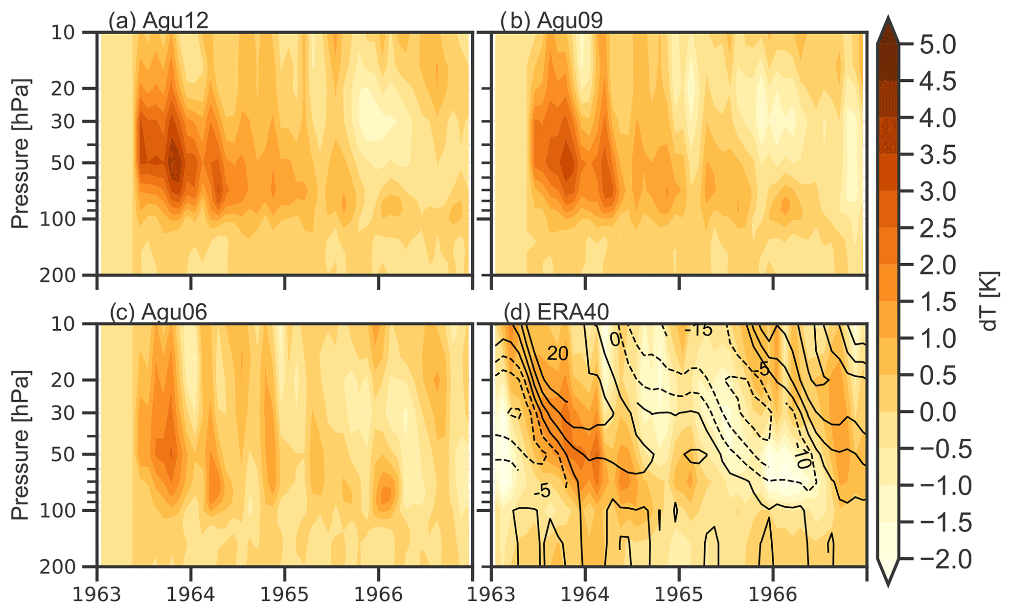
We have applied the interactive stratospheric aerosol configuration of the UM-UKCA model to simulate the formation and global dispersion of the volcanic aerosol clouds from the three largest tropical eruptions of the 20th century: Agung, El Chichón, and Pinatubo. The simulations are analysed to assess the evolution of each eruption cloud, from an initial tropical reservoir of volcanic aerosol to a hemispherically dispersed stratospheric aerosol cloud. For each eruption, three-member ensembles are carried out for the upper, lower, and mid-point of the literature range of SO₂ emission, aligning with the design of the co-ordinated HErSEA experiment, part of the multi-model ISA-MIP interactive stratospheric aerosol modelling initiative (see Timmreck et al., 2018). The analysis is also designed to provide new “microphysically consistent and observationally constrained” volcanic forcing datasets for climate models to represent each eruption's surface cooling more realistically.

Simulated aerosol optical properties are compared against a range of satellite datasets. The model captures the observed variation in global stratospheric sulfur from 1991 to 1993 HIRS measurements very well, and experiments Pin10 and Pin14 define a model-specific 10 to 14 Tg emissions uncertainty range and identify a potential weighting to define a best-fit forcing dataset for Pinatubo. Our simulations also show that the aerosol decay rate is inversely proportional to the SO₂ injection amount, illustrating how increased aerosol particle size causes faster sedimentation. The model ensembles compare very well to mid-visible and near-infra-red aerosol extinction from SAGE-II measurements, although the model has an sAOD high bias in the tropics, a common feature seen in interactive stratospheric aerosol models (e.g. Niemeier et al., 2009; Mills et al., 2016; Sukhodolov et al., 2018). We have also compared the Pinatubo ensembles to the three widely used forcing datasets (CMIP6–GloSSAC, Sato, and Ammann), and we find that the Pin14 model ensemble shows overall best agreement. A plateau in lower-stratospheric tropical extinction seen in CMIP6-GloSSAC data for almost 1 year after the Pinatubo eruption is not reproduced in our simulations and thus remains an open scientific question. The 10–14 Tg SO₂ emissions range for the model is lower than the 14–23 Tg observed to be present after the eruption (Guo et al., 2004b), and the tropical sAOD₅₅₀ high bias is consistent with the models missing an important removal process. Plausible suggestions for these are (a) the vertical re-distribution of the volcanic cloud due to ash, (b) changes in SO₂ oxidation due to OH decrease inside the plume, and (c) too strong a sub-tropical barrier in the models.

The simulated R_eff shows good agreement with CMIP6-GloSSAC data, although the model simulates a deeper global layer of enhanced SAD than in the 3λ dataset (Luo, 2016). Simulated global-mean SW forcing (solar dimming) in run Pin10 shows excellent agreement with the magnitude of the anomaly in the ERBE data, and the LW forcing in the model also matches well with the magnitude and shape of the ERBE anomaly. Assuming a 1 K colder temperature anomaly in ERA-Interim tropical temperatures due to the downward-propagating QBO, a warming of 3 K near 50 hPa is well simulated in both Pin10 and Pin14 simulations. Overall, most of the comparisons suggest that about 10–14 Tg SO₂ injection between 21 and 23 km is sufficient to simulate the climate and chemical impact of the Mt Pinatubo eruption.

For the El Chichón eruption, there are significant differences between observation-based sAOD₅₅₀ estimates, hence evaluation of the simulations is somewhat restricted. However, NH mid-latitudes generally have a good-quality observational data record, and sAOD₅₅₀ from run Elc05 shows good agreement with CMIP6 and, in the tropics model, compares better with Sato dataset. Our extinction comparisons also show that there are clear inhomogeneities in the CMIP6-GloSSAC data during this period; hence El Chichón-related aerosol properties must be treated with caution. Based on comparisons of the lower-stratospheric warming of about 2 K, 5 and 7 Tg SO₂ injections seem to be reasonable lower and upper limits for what is required to simulate observed temperature changes.

Finally, the evaluation of Mt Agung aerosol is more complicated due to much larger differences in the observation-based datasets. Due to the westerly phase of QBO and timing of the eruption, CMIP6 data show a tropical peak in sAOD₅₅₀ within 1 month of the March eruption which is transported to SH mid-latitudes by October. The Sato dataset suggest two peaks in the tropics 8 and 14 months after the eruption. Run Agu06 shows reasonable agreement with the limited amount of observational extinction data, although that is not conclusive. Comparison with the lidar measurements from Lexington suggests that the UM-UKCA simulated vertical extent of the Agung cloud in the NH mid-latitudes is in best agreement for Agu09. Comparisons with ERA-40 temperature anomalies also suggest 3 K warming in the tropical stratosphere (2 K in the model simulation due to westerly phase of QBO). Assuming CMIP6-simulated sAOD₅₅₀ is realistic, 6 and 9 Tg SO₂ injection seems to be the best lower and upper estimates required to simulate Mt Agung-related aerosol in the UM-UKCA.

Overall, we have validated the interactive stratospheric aerosol configuration of the GA4 UM-UKCA model and have shown that the simulated aerosol properties for the Pinatubo ensemble are consistently in good agreement with a range of satellite-based observational datasets. For Pinatubo, we have also compared to three different independent tests of the radiative effects from the volcanic aerosol cloud: the ERBE flux anomaly time series in the SW and LW and the stratospheric warming in the ERA-Interim reanalysis. These comparisons confirm that a 10 to 14 Tg emission flux of SO₂ would accurately represent the effects that the new forcing datasets would enact for Pinatubo in CCM integrations. For El Chichón and Agung, the magnitude of the volcanic forcing is highly uncertain, the volcanic aerosol datasets used in CMIP5 and CMIP6 historical integrations showing substantial differences. We contend there is substantial potential to improve on this situation, by identifying consensus forcings from multi-model simulations (Timmreck et al., 2018), with comparison to additional in situ and active remote-sensing measurements such as those being initiated within the SSiRC data rescue activity (Antuña Marrero et al., 2020b; Mann et al., 2020).