the Creative Commons Attribution 4.0 License.
the Creative Commons Attribution 4.0 License.
 | 11 Nov 2020
Evaluation of climate model aerosol trends with ground-based observations over the last 2 decades – an AeroCom and CMIP6 analysis
Jonas Gliß
Michael Schulz
Wenche Aas
Elisabeth Andrews
Huisheng Bian
Mian Chin
Paul Ginoux
Jenny Hand
Brent Holben
Hua Zhang
Zak Kipling
Alf Kirkevåg
Paolo Laj
Thibault Lurton
Gunnar Myhre
David Neubauer
Dirk Olivié
Knut von Salzen
Ragnhild Bieltvedt Skeie
Toshihiko Takemura
Simone Tilmes
This study presents a multiparameter analysis of aerosol trends over the last 2 decades at regional and global scales. Regional time series have been computed for a set of nine optical, chemical-composition and mass aerosol properties by using the observations from several ground-based networks. From these regional time series the aerosol trends have been derived for the different regions of the world. Most of the properties related to aerosol loading exhibit negative trends, both at the surface and in the total atmospheric column. Significant decreases in aerosol optical depth (AOD) are found in Europe, North America, South America, North Africa and Asia, ranging from −1.2 % yr−1 to −3.1 % yr−1. An error and representativity analysis of the spatially and temporally limited observational data has been performed using model data subsets in order to investigate how much the observed trends represent the actual trends happening in the regions over the full study period from 2000 to 2014. This analysis reveals that significant uncertainty is associated with some of the regional trends due to time and space sampling deficiencies. The set of observed regional trends has then been used for the evaluation of 10 models (6 AeroCom phase III models and 4 CMIP6 models) and the CAMS reanalysis dataset and of their skills in reproducing the aerosol trends. Model performance is found to vary depending on the parameters and the regions of the world. The models tend to capture trends in AOD, the column Ångström exponent, sulfate and particulate matter well (except in North Africa), but they show larger discrepancies for coarse-mode AOD. The rather good agreement of the trends, across different aerosol parameters between models and observations, when co-locating them in time and space, implies that global model trends, including those in poorly monitored regions, are likely correct. The models can help to provide a global picture of the aerosol trends by filling the gaps in regions not covered by observations. The calculation of aerosol trends at a global scale reveals a different picture from that depicted by solely relying on ground-based observations. Using a model with complete diagnostics (NorESM2), we find a global increase in AOD of about 0.2 % yr−1 between 2000 and 2014, primarily caused by an increase in the loads of organic aerosols, sulfate and black carbon.
- Article
(5363 KB) - Full-text XML
-
Supplement
(144 KB) - BibTeX
- EndNote


As one of the key gears involved in the climate mechanism (Pöschl, 2005) and as a predominant component of air quality that affects human health (Burnett et al., 2014), aerosols have been increasingly subject to observation over the last 2 decades, both from ground- and space-based platforms (Holben et al., 2001; Kaufman et al., 2002). Aerosols are also recognized to have an important role in the fertilization of the Amazon forest (Yu et al., 2015), and in other socioeconomic fields such as solar energy production (Li et al., 2017; Labordena et al., 2018; Sweerts et al., 2019).
Through their direct, semidirect and indirect effects (Rap et al., 2013; Johnson et al., 2004; Lohmann and Feichter, 2005), aerosol particles are crucial for the estimation of radiative forcing. Currently, the overall estimate of aerosol radiative forcing is associated with high uncertainties (Haywood and Boucher, 2000; Stocker et al., 2014). Some of the reasons for these uncertainties reside in the heterogeneity of atmospheric particles, in terms of both their microphysical and their optical properties, as well as in terms of the high variability in these aerosols in space and time. Different regions of the world exhibit contrasting aerosol properties (Holben et al., 2001), which can vary depending on the seasons, from year to year, and possibly exhibit interannual trends (Streets et al., 2009). In addition to natural emissions such as sea salt and dust, anthropogenic sources of aerosols add another layer of complexity. The second industrial revolution, which relied on the use of fossil fuel energy, has had a significant impact on the aerosol load on a global scale and on the local air quality, resulting in severe pollution episodes, such as the famous 1952 smog event in London (Bell et al., 2004) that caused the deaths of thousands of people within a few days. Starting in the 1970s in the USA and in the 1990s in Europe, mitigation measures were implemented to limit the emission of particles and other pollutants (Bryner, 1995; Turnock et al., 2016), resulting in significant improvements in terms of air quality and particle concentration levels (Likens et al., 2001). In recent decades there has been a shift in anthropogenic emissions from Europe and North America to the developing nations, which are now facing, in varying degrees, the air quality issues that affected Europe and North America 40 years ago (Streets et al., 2008; Ramachandran et al., 2012).
In order to provide realistic radiative-forcing estimates and projections, it is important for the atmospheric models to be able to capture the long-term aerosol trends caused by both natural and anthropogenic variations.
Assessing and improving the modeling of aerosols in global Earth system models is the main objective of the AeroCom project. Specific experiments are conducted within this initiative with a focus on individual aerosol species, such as dust (Huneeus et al., 2011) or organic aerosols (Tsigaridis et al., 2014), while dedicated control experiments aim to enable an assessment of global aerosol modeling. Both Kinne et al. (2006) and, more recently, Gliß et al. (2020a) present evaluations of simulations of global aerosol optical properties by focusing on AeroCom control experiment data for a specific year.
This study presents an overview of the aerosol trends for multiple aerosol parameters (optical and chemical) over the last 2 decades using ground-based observation network data as a reference for the evaluation of the models' skills in reproducing those trends.
To serve that purpose, this study addresses the following two questions:
-
What are the observed aerosol trends over the last 2 decades in the different regions of the world (Sect. 4.1)?
-
Can the climate models reproduce these observed trends (Sect. 4.2)?
Then, having developed an understanding of the models' skills in reproducing the observed aerosol trends, the last section of this study aims to answer the following question:
-
What are the global aerosol trends derived from the model data (Sect. 4.3)?
The CAMS reanalysis dataset and output from six AeroCom models and four CMIP6 models (both model groups performed historical experiments) are evaluated in this work. CMIP6 (Coupled Model Intercomparison Project, Phase 6) is an intercomparison project organized by the WCRP (World Climate Research Programme). Participating models will contribute to the assessment of climate change in the upcoming 2024 IPCC (Intergovernmental Panel on Climate Change) report.
Figure 1 presents the time series of modeled global AOD (aerosol optical depth) between 1850 and 2014. All of the climate models appear to exhibit a large increase in AOD, especially between 1950 and 1990 (Tegen et al., 2000), followed by more stable conditions up to the present. While the models show some diversity in absolute values, the trends (focus of this paper) seem to be consistent among the different models at a global scale. Long-term monitoring of many optical and chemical parameters was initiated in the late 1990s (e.g., Holben et al., 2001; Laj et al., 2020), providing a high-quality dataset for the investigation of aerosol trends over the last 2 decades (e.g., Collaud Coen et al., 2020; Hand et al., 2019a; Aas et al., 2019). These observational datasets also offer an opportunity to validate the modeled trends in this period. Since 2014 is the last year available from the CMIP6 historical runs, we focus this study on the aerosol trends in the 2000–2014 period.
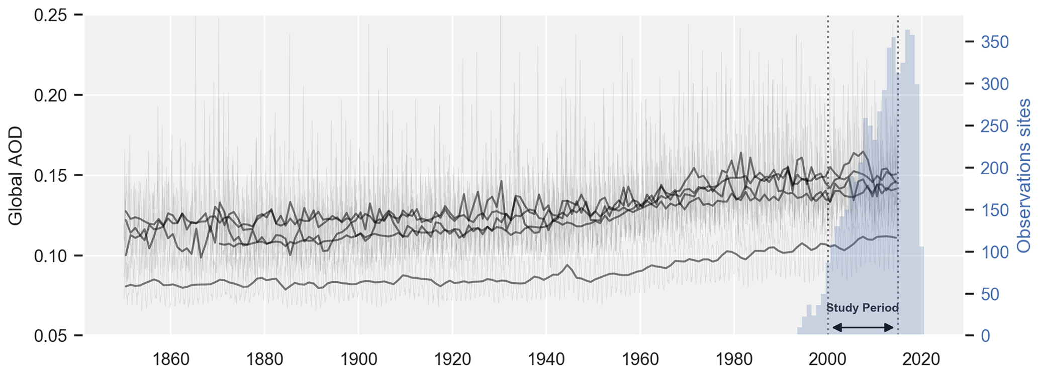
Figure 1Global AOD computed from model historical runs (Oslo CTM3, GFDL-AM4, CanESM5, CESM2, IPSL-CM6A, ECHAM-HAM) at monthly (gray lines) and yearly (black lines) resolutions, overlaid with the number of active observation sites in the AERONET sun photometer network.
A set of nine columns and in situ surface aerosol datasets are used in this study. The observation networks and the models providing output for these parameters are reported in Table 1.
Table 1List of observations and model datasets used in this study (see text for explanation).
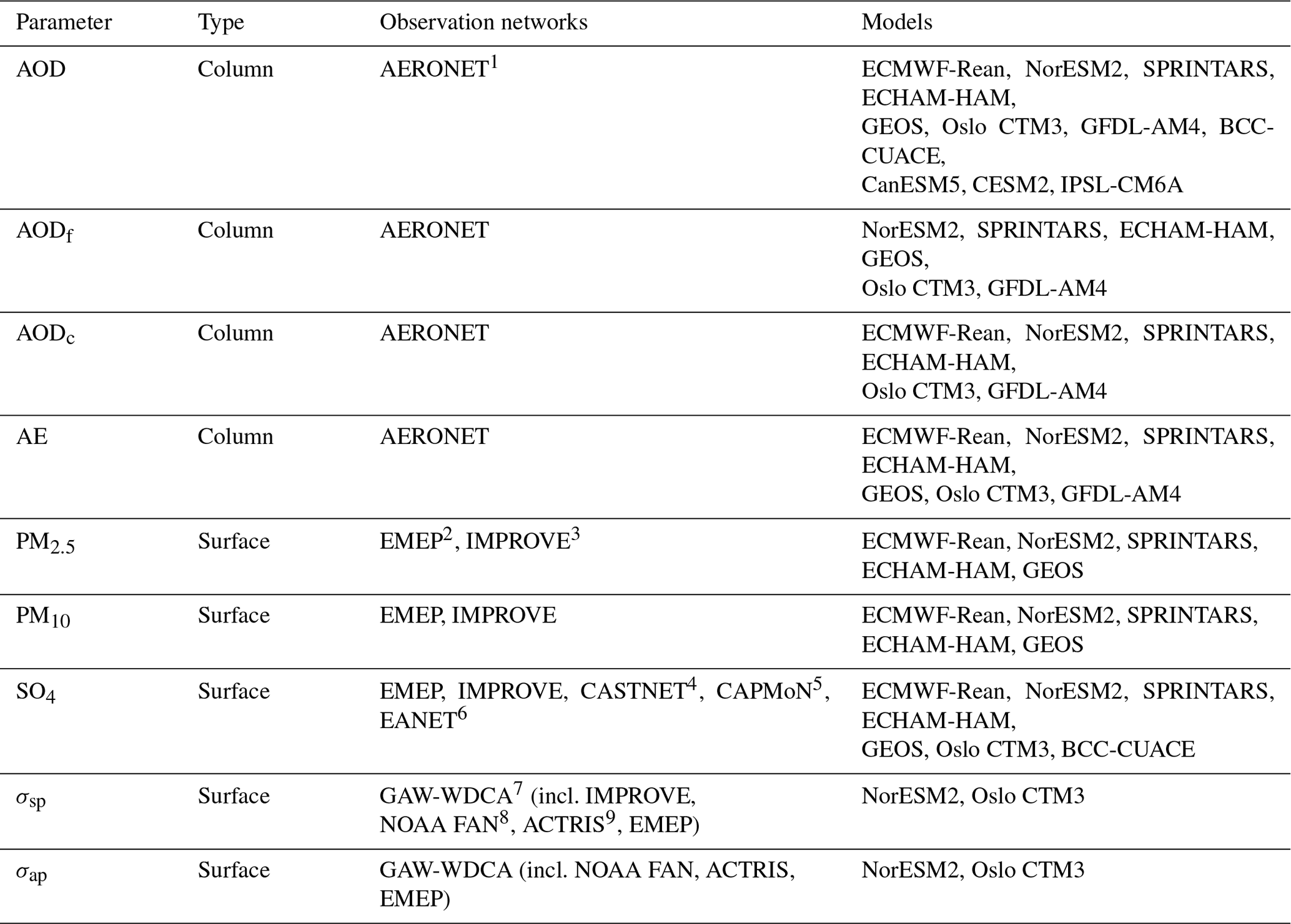
1 Aerosol Robotic Network. 2 European Monitoring and Evaluation Programme. 3 Interagency Monitoring of Protected Visual Environments. 4 Clean Air Status and Trends Network. 5 Canadian Air and Precipitation Monitoring Network. 6 Acid Deposition Network in East Asia. 7 Global Atmosphere Watch – World Data Centre for Aerosols. 8 National Oceanic and Atmospheric Administration Federated Aerosol Network. 9 Aerosol, Clouds, and Trace Gases Research Infrastructure.
2.1 Observations
For each of the parameters used in this study, data of the highest quality level provided by the different observation networks were used. Mountain sites, corresponding to an elevation above 1000 m, were excluded, mainly because global models have problems simulating the aerosol distribution in complex terrain (Kinne et al., 2013).
2.1.1 Columnar aerosol optical properties
The Aerosol Robotic Network (AERONET) is a network that was established by NASA (National Aeronautics and Space Administration) and has been expanded by national and international collaborations. AERONET operates aerosol ground-based measurements in the different regions of the world (Holben et al., 2001). Observation of the columnar aerosol properties is performed by standardized and calibrated solar-powered Cimel Electronique sun photometers. These instruments measure the solar radiation reaching the surface of the Earth at different wavelengths and for different optical geometries. A new version of the sun photometer (CE318-T) is also able to perform nighttime measurements using the moon as a light source (Barreto et al., 2016). The direct measurements (aiming at the light source) allow for the derivation of the aerosol optical depth (AOD) and the Ångström exponent (AE), which are related to the number and size of the particles, respectively. The spectral information can be further utilized to derive the AOD for the fine and the coarse particles, split by diameters less than or greater than 1.2 µm (O'Neill et al., 2003). Three different data quality levels are available depending on the application of cloud filtering and correction for instrument calibration derivations (Smirnov et al., 2000, 2004). The level 2.0 version 3 daily data, which provide automatic instrument anomaly quality controls (Giles et al., 2019), are used in this study for four different parameters: AOD (calculated at 550 nm); AE (calculated using 440 and 870 nm channels); and AODf (or fine AOD) and AODc (or coarse AOD), corresponding to the AOD of the particles whose diameter is less than and greater than 1.2 µm, respectively.
2.1.2 Particulate matter concentrations
The particulate matter (PM) measurements are from EMEP (covering Europe) and IMPROVE (for North America). The PM data have been made available either via the EBAS database infrastructure (http://ebas.nilu.no, last access: 26 October 2020) or in the original IMPROVE data to be found in the VIEWS database (http://views.cira.colostate.edu, last access: 26 October 2020). Both PM10 and PM2.5 (in µg m−3) are used in this study. Note that the PM10 size fraction of particles below 10 µm encompasses the PM2.5 aerosol mass below 2.5 µm.
The first PM measurements in EMEP started in 1996, and the number of sites increased steadily in the following decade (Tørseth et al., 2012). Most of the sites use the gravimetric method for both size fractions, though some have used automated monitors, i.e., tapered element oscillating microbalance (TEOM) and filter dynamics measurement system (FDMS) or beta attenuation. The EMEP monitoring complies with European standards, i.e EN 12341:2014 for the gravimetric methods and EN 16450:2017 for the automatic methods.
The IMPROVE network has been operating since 1988 at predominantly remote and rural sites across the United States. This ensures a good representativity of the measurements as some chemical species contributing to PM observations (i.e., organic carbon) can exhibit different seasonality and spatial variability. IMPROVE uses four separate modules to collect samples for speciated PM2.5 analysis and gravimetric PM2.5 and PM10 bulk mass measurements. Samples are collected every third day for 24 h and reported at local conditions. PM2.5 and PM10 mass concentrations are determined from Teflon filters from two separate modules sampling with PM2.5 and PM10 inlets, respectively. The gravimetric mass measurements are not performed at controlled relative humidity and temperature, and a laboratory relocation in 2011 resulted in unstable weighing conditions. Therefore, gravimetric mass measurements from 2011 to 2018 were subject to potentially high-relative-humidity conditions and likely contain particle-bound water on the filters that could bias trends (Hand et al., 2019b).
2.1.3 Sulfate aerosol concentration
The sulfate aerosol (SO4) concentration dataset is a subset of the global data presented in Aas et al. (2019) and is based on measurements obtained in different regional networks as described in Table 1. The sulfate aerosol concentrations are obtained from analysis of aerosol filters. In the EMEP, CASTNET, CAPMoN and EANET networks, these are sampled with either a PM10 inlet or a total aerosol inlet, with no specific-size cutoff effective, using a filter pack sampler. In the IMPROVE network, sulfate measurements are carried out using a filter pack sampler with a PM2.5 inlet. The filters are typically analyzed by ion chromatography after water extraction of the aerosol filter.
The data have been screened to be of satisfactory quality. Urban sites are not included and nor are sites where the surroundings have changed considerably in the period in question. In Aas et al. (2019) the data were averaged to monthly means. When the data have a lower sampling frequency than daily, samples are weighted prior to averaging in accordance with how many days were sampled in a given month.
2.1.4 Scattering and absorption coefficients
For the surface in situ PM measurements, the scattering and absorption coefficient measurements were accessed through EBAS database infrastructure. The level 2 data (quality controlled, hourly averaged, reported at standard temperature and pressure – STP – conditions) were used. Detailed information on the quality assurance and quality control procedures for GAW aerosol in situ data is available in Laj et al. (2020). The difference in measurement conditions (i.e., observations being made at STP versus models simulating at ambient conditions) was not expected to impact the calculated trends, so no adjustment was made to account for this.
Scattering and absorption coefficients are measured by different instruments:
-
Scattering coefficients (σsp; in Mm−1) were measured by integrating nephelometers. For better consistency in the model comparisons (model data for these parameters are reported for RH = 0 %), only the measurement data obtained when the relative humidity in the instrument was lower than 40 % were utilized (Pandolfi et al., 2018).
-
Absorption coefficients (σap; in Mm−1) were obtained from filter-based absorption photometers.
Due to the scarcity of stations available for long-term trend analysis (only 28), the presence of regionally nonrepresentative stations (e.g., stations located near roads, in cities), difficult to capture by global models, can have large effects on the computation of the regional-average time series. The urban stations have therefore been removed from this analysis.
Altogether the same data selection procedures (exclusion of stations, removal of outliers) and corrections (conversion to coefficients at 550 nm wavelength) were applied as in Gliß et al. (2020a), which describes the AeroCom evaluation of the 2019 control experiment, analyzing AeroCom simulations of the year 2010 in detail.
2.2 Models
A set of 10 climate and aerosol models and an aerosol reanalysis dataset are used in this study. Their main characteristics are reported in Table 2. These models can be separated into three main groups.
Inness et al. (2019); Zhang et al. (2009)Takemura et al. (2000, 2002, 2005)Tegen et al. (2019); Neubauer et al. (2019)Bian et al. (2017); Chin et al. (2002); Colarco et al. (2010)Lund et al. (2018); Myhre et al. (2009)Zhao et al. (2018a, b)Zhang et al. (2012, 2014); Wang et al. (2014)Seland et al. (2020); Kirkevåg et al. (2018)Swart et al. (2019) (2019)Lurton et al. (2019)Table 2Information on models used in this study (CAMS-Rean: CAMS reanalysis, AP3: AeroCom phase III, CMIP6: historical experiments from CMIP6).
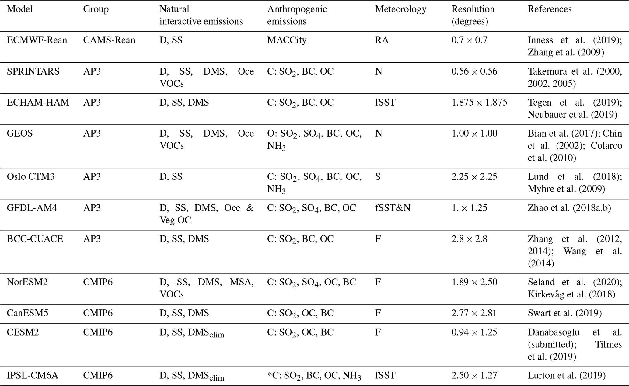
Anthropogenic emissions (C = CMIP6 CEDS; O = other; *C = CMIP6 modified); natural interactive emissions (D = dust; SS = sea salt; O = biogenic organic; V = volcanic; Oce = oceanic; Veg = vegetation; DMS = dimethyl sulfide; DMSclim = dimethyl sulfide from climatology; VOCs = volatile organic compounds, MSA = methane sulfonate); meteorology (S = prescribed varying meteorology CTM (chemical transport model); N = GCM (general circulation model) nudged to analyzed meteorology; fSST (fixed sea surface temperature) = fixed SST (sea surface temperature) − SIC (sea ice concentration) monthly fields, GCM not nudged; F = free-running coupled GCM; RA = combined reanalysis of meteorology and composition).
2.2.1 CAMS reanalysis
The CAMS reanalysis, which is the successor to the MACC (Monitoring Atmospheric Composition and Climate) reanalysis, is the latest global reanalysis dataset of atmospheric composition produced by the Copernicus Atmosphere Monitoring Service (Inness et al., 2019). It is produced using 4D-Var data assimilation in the CY42R1 model cycle of the ECMWF (European Centre for Medium-Range Weather Forecasts) Integrated Forecast System (IFS), with 60 hybrid sigma–pressure vertical levels. The model used in the CAMS reanalysis includes several updates to the aerosol and chemistry modules on top of the standard CY42R1 release. The IFS model assimilates several satellite products, from aerosols (AOD) to greenhouse gases (CO2, CH4; Inness et al., 2019), whereof most relevant for aerosol trends are data from both MODIS sensors and AATSR and ATSR-2. Daily data, from the ECMWF data archive (MARS), were used in this study. The CAMS reanalysis dataset covers the period January 2003 to near real time. The first 3 years of this study period (2000–2002) are missing for this model.
2.2.2 AeroCom phase III
Initiated in 2000, the AeroCom project (https://aerocom.met.no, last access: 26 October 2020) is an open international initiative of scientists interested in the advancement of the understanding of global aerosols and their impact on climate (Schulz et al., 2006). Different model experiments have been conducted during the third phase of this project, started in 2015, in order to investigate not only specific topics (e.g., dust, volcanic aerosols, aerosol absorption, hygroscopicity) but also the general modeling of the aerosols (control experiments). The model versions and parametrizations used in AeroCom are closely linked to the versions used for CMIP6 and, for instance, AerChemMIP (Aerosol Chemistry Model Intercomparison Project) climate experiments.
In this study, we use the model outputs from the historical AeroCom experiment, whose main aim is to understand the regional trends in aerosol distribution from 1850 to 2015 and to quantify the aerosol forcing with a main emphasis on the direct aerosol effect. The models were also run in various configurations, providing different degrees of constraints on the evolving meteorological conditions, such as using monthly fixed sea-surface temperature (SST); historically evolving SSTs; and basic meteorology fields, e.g., wind for a given year.
2.2.3 CMIP6
The upcoming 2024 IPCC sixth assessment report (AR6) will feature new state-of-the-art CMIP6 models with model runs in higher resolution and with new physical processes. An overview of the experimental design and organization can be found in Eyring et al. (2016). In this study, we use a preliminary extract of the data of four CMIP6 models from the historical experiment, as available on ESGF (Earth System Grid Federation) nodes (https://esgf.llnl.gov, last access: 26 October 2020), which provided output from 1850 to 2014. The last year of the study period of the analysis presented here was selected as 2014.
3.1 Regional time series
Due to the nature of the processes involved in the emission and the deposition of aerosols, one can expect different trends in different regions of the world. Instead of investigating the trends obtained at each individual observation station in a given region, we resort here to the analysis of average regional time series as computed by assembling all measurements at stations in each region. One advantage of this method is that a single trend can be computed in a given region, with an associated significance and uncertainty. It is difficult, apart from in a diversity analysis, to define such an uncertainty when combining individual trends. Also, with our aggregation method, even a station that has not provided a sufficient number of data for computing a trend at its location can still contribute to the computation of a regional time series. The computation of such aggregated regional time series makes most sense in regions exhibiting similar seasonal patterns.
3.1.1 Region definition and observation coverage
Seven regions are considered in this study. The definition of these regions has been determined in a pragmatic way to limit the number of geographic areas investigated, but altogether it also provides global coverage when considering the ensemble of all regions. The Americas and Africa have been separated into northern and southern sections. In order to assemble the sites most affected by Saharan dust, the North Africa region has been extended to the north beyond the continent itself. Stations located in the south of Spain, Cyprus and Greece contribute to the regional time series in the region we are calling North Africa. The regions' coordinates can be found in the Supplement.
As seen in Fig. 2, the regions do not have similar coverage in terms of observations. North America and Europe have the highest concentrations of instruments monitoring aerosol trends.
-
AERONET is the most important network in terms of number of instruments. More than 1000 observation points, with more or less long time series, are found across the globe. The highest density of instruments is in Europe and in the central part of North America (USA). The lowest densities are found in southern Africa and Australia.
-
For particulate matter, 227 instruments are used in this study and are spread mostly over Europe and North America.
-
For SO4, 346 instruments altogether have been operating, mostly in North America and Europe. A few stations are also located in Asia and North Africa.
-
For both parameters σsp and σap combined, approximately 50 stations are spread over North America, Europe, North Africa and Asia. Due to time coverage issues (2005 is the first year where in situ optical data are available in the European time series), the data from 2000 up to the year 2018 were used to compute the regional time series of these two parameters.
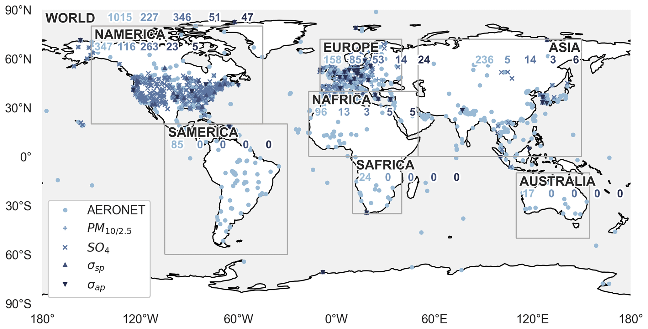
Figure 2Distribution of the observations within the different regions considered in this study. The numbers reported within each region correspond to the maximum number of stations given for the observation networks, corresponding to the five observation types found in the legend.
3.1.2 Time series aggregation requirements
The regional time series are computed by combining, for each month, the valid data of all the stations in the corresponding region. In order to construct consistent and robust regional time series, some additional criteria are required to be met to provide a valid point (a station with valid measurements) for the regional time series. Stations with very short time series (e.g AERONET DRAGON campaign stations) are eliminated by requiring a minimum of 300 valid daily measurements in the whole period from 2000 to 2014, which reduces, as an illustration, the number of AERONET stations from 1015 to 437. A minimum of three valid stations is required to be present in the overall regional time series to produce a valid point. In other words, if the available time resolution is daily, at least three stations need to provide valid data for a certain day in order to produce a valid regional mean for that day. The list of the station names contributing to the computation of the regional time series can be found in the Supplement.
When all criteria are fulfilled for a given month in the regional time series, the median and the first and third quartiles are computed from all valid data points available. The quartiles provide an indication of the intraregional variability. An example of regional time series is shown in Fig. 3 for AOD.
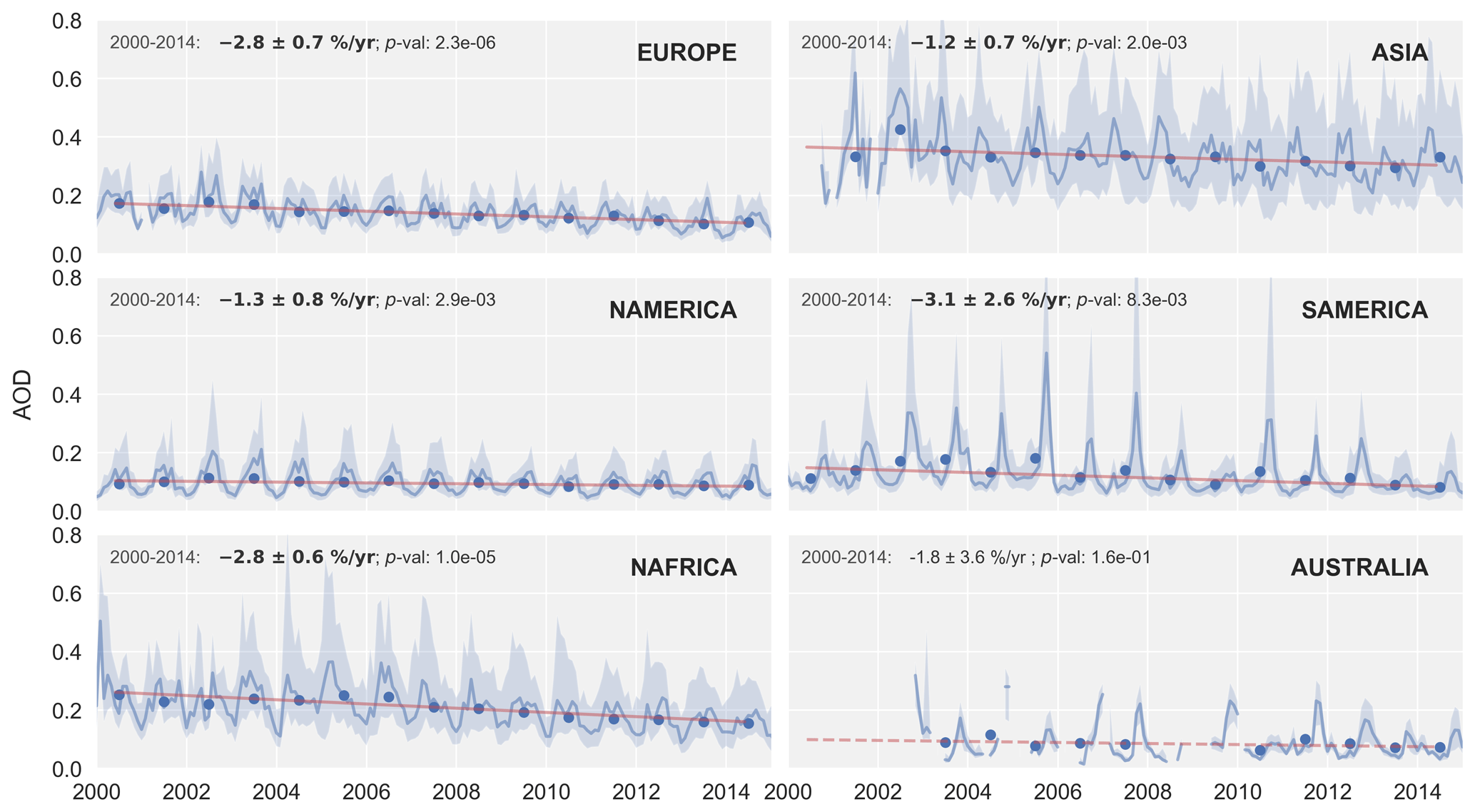
Figure 3Regional time series of AOD. The dark blue line corresponds to the median, and the light blue envelope is bound by the first and third quartiles of all valid points at the corresponding month, respectively. The blue dots correspond to the yearly averages which are used to compute the linear trend. The latter is displayed as a continuous line when the trend is significant and as a dashed line when it is not. Trend values, an error estimate and a significance value are given in each panel.
3.2 Trends calculation
3.2.1 Yearly regional time series
For all of the parameters, the trends are computed based on the yearly averages of the regional time series. Using the yearly averages eliminates any issues caused by the seasonal cycles (observed for most of the aerosol parameters used in this study) during the calculation of the trend slope. In order to ensure the statistical robustness of these yearly averages, the time averaging is performed step-by-step with specific time constraints. By starting at the finest time resolution available in the data, monthly, seasonal and then yearly averages are computed when the following criteria are fulfilled:
-
at least 5 d per month are available (when daily observations are available)
-
at least 1 month with data per season is present (seasons defined as JFM, AMJ, JAS, OND)
-
all four seasons are available for a given year.
These temporal constraints offer a reasonable compromise between the availability and robustness of the yearly statistics.
3.2.2 Trends computation
We use the same methodology as described by Aas et al. (2019) to derive the trends in the regional time series. The significance of the trends is tested with the Mann–Kendall test (Hamed and Rao, 1998). The related p value is used to determine if the trend is significant or not within a confidence interval of 95 %. The slope is calculated with the Theil–Sen estimator, which is less sensitive to outliers than standard least-squares methods (Sen, 1968). At least seven valid yearly regional averages (50 % of time coverage) are required in the regional time series for the computation of a slope.
An uncertainty is provided for each trend by combining the error in the slope calculation itself with the error in the residuals:
where Δ m is the Theil–Sen estimator 95 % confidence interval, y(2000) is the value of the regression line at the year 2000, m is the value of the Theil–Sen slope, and Δr is the averaged error in the residuals computed based on the difference between the linear trend and the yearly mean values of the regional time series.
The trend is provided as a relative trend (% yr−1) with respect to the first year of the time period (2000).
3.3 Representativity of the trends
The number of available points used to compute the regional time series is not constant in time. For a given observation station, the number of points available might vary in time due to the nature of the measurements. For instance, classic sun photometers only measure in the daytime and in cloud-free conditions. Due to seasonal daylight and cloud condition variations, clear seasonal cycles are observed in the number of observations of AOD. The density of the different observation networks can also change with time. The early development of the different observation networks usually coincided with an increase in the number of observation stations. More recently, primarily for funding reasons, some networks have reduced the number of stations. This variation in the number of available measurements raises the question of time representativity for the computation of the trends.
Associated with this time representativity issue is the space representativity issue. The data coverage is uneven across the different regions. Moreover, within a single region, the observation stations might be located in contrasting environments. Stations located in environments that are more urban, more rural or mostly affected by natural particles might have trends differing from the trend associated with the whole region.
Some studies have focused on the representativity of the observation stations by investigating the biases of different optical properties (Wang et al., 2018; Schutgens et al., 2017; Schutgens, 2019). The analysis here is dedicated to characterizing the representativity of the observation networks specifically for the purpose of computing the trends. These two perspectives on representativity might give different results, since a station associated with a bias could still have a representative tendency in time. In order to evaluate the effect of the partial space and time sampling of the observations for the evaluation of the trends, two sensitivity studies, focusing on the time sampling and the space sampling, have been conducted using NorESM2 model data subsets. For each of these studies, the trends are computed for one reference (Ref) and one experiment (Exp) dataset and compared with each other. The reference dataset corresponds to the model data co-located with the available observations, while the experiment dataset uses all model points.
-
Time representativity study.
- –
For Reftime, model data are co-located in space and time with available observations.
- –
For Exptime, model data are co-located in space with available observations using the complete model time series.
- –
-
Space representativity study.
- –
For Refspace, model data are co-located in space with available observations using the complete model time series (= Exptime).
- –
For Expspace, all of the model grid points in the region use the complete model time series.
- –
The difference between the relative trends is computed for each parameter and region. In order to summarize the representativity, those differences are then converted into a score (%) by using a mapping function which has been defined based on a normal distribution. The choice of the parameters describing this function leads to a representativity score of 100 % when there is no difference in the trends computed for a reference and an experiment dataset, while a difference of 0.5 % yr−1 obtained with these two datasets would indicate a representativity score of 50 %. Finally, the total score is computed as the mean of the time and the space representativities.
An example of the calculation is presented in Fig. 4 for AOD in Europe and North America. In both regions, the Reftime dataset, corresponding to the available observations, reveals strong seasonal cycles when considering the number of points used to compute the regional time series. These cycles are observed with most of the sun photometer datasets since the instruments only operate during daytime and cloud-free conditions and the amount of daylight and cloud varies with the season. Together with this seasonal cycle, one observes an increase in the number of points with time, which reflects the increasing number of stations over these two regions.

Figure 4Three regional AOD time series and respective trends, constructed from model data (NorESM2) for the investigation of the representativity of the observational data. Panels (a) and (b) correspond to the number of points used to compute the regional time series for the three different datasets. Panels (c) and (d) show the time series, the trends and the resulting representativity value (black, bold). The blue color (Reftime) corresponds to the model output co-located in space and time with the available observations. Panels (a) and (b) show an overall increase in the number of available observations (more stations) combined with a seasonal cycle (less AOD available in wintertime). The orange color (Exptime∕Refspace) corresponds to the model output co-located in space with the stations providing measurements, using the complete time series from 2000 to 2014. The green color (Expspace) corresponds to the model output in the whole geographic region (see Fig. 2), using all of the grid boxes without any co-location with the observations.
The trends in Europe show similar values for the time study, which means that the trend is not greatly affected by the variation in the available measurements in time. The difference is larger when considering all the grid boxes of the domain, but the overall difference in the two studies corresponds to a representativity of 76 %. In North America, the difference in the three trends is larger, particularly for the space study trend. This means that the trend obtained in the whole region is significantly different from the trend obtained when considering only the grid points where observation stations are located. It should be mentioned that the ocean grid points are not filtered out when computing the trends over the whole domain. For this reason, the regions containing a greater proportion of ocean grid points, where the trends are most likely to differ from those observed over land, will tend to have a lower spatial representativity, such as in North America.
This representativity study illustrates that the partial coverage in time and space of the observations leads, in some cases, to artificial trends. The representativity scores are discussed for each parameter in the following section together with the trend estimate results.
4.1 Trends in observations
This section presents the trends in the observations computed for the different parameters and over the predefined regions. In order to compare the trends observed for the set of nine aerosol parameters in a consistent manner, we focus on the relative trends, with the reference set to the year 2000 as the first year of the study period. The means for the year 2000, reported in Table 3, reveal a large interregional variability.
Table 3Observational mean values for the year 2000, the reference year used for computing relative trends. Each value is extracted as the intercept of the linear trend computed in the 2000–2014 period, except for σsp and σap, where the trends have been computed over 2000–2018. Because the required minimum number of yearly averages was set to seven, no trend could be computed in the southern African region.

The AOD is more than 3 times higher in Asia (AOD = 0.37) than in North America and Australia (AOD = 0.10). Intermediate AOD values are found in Europe and South Africa, while the second-highest load is found in North Africa (AOD = 0.26). In most regions, the AOD is largely dominated by its fine-mode fraction (AODf), but this is not the case in North Africa (or Australia), where the persistent presence of desert dust makes the coarse-mode (AODc) contribution to the total AOD similar in size to the fine-mode contribution. This predominance of coarse particles is reflected in the AE values which exhibit lower values in North Africa (AE = 0.70) and Australia (AE = 1.00).
The PM observations are primarily available from Europe and North America. PM10 observations are also available in the North Africa region as defined in this analysis, but these stations are located in the northern part of the region, i.e., in southern Europe, which is less affected by the dust sources than the AERONET stations, which cover the whole region including the surrounding deserts. Both PM10 and PM2.5 are larger in Europe than in North America, with different relative proportions. In Europe, PM2.5 represents 76 % of the PM10, as compared to only 57 % in North America. This difference in the relative proportion of fine particles against coarse particles in Europe and North America may be due in part to our definition of regions. Putaud et al. (2010) presented a phenomenology of PM data in Europe showing coarse aerosols tended to be highest in southern Europe which in our study is part of the North Africa region. The discrepancy in the relative proportions of coarse and fine aerosols in Europe and North America may be exacerbated both by a decrease in North America of the fine-particle concentration due to pollution mitigation strategies and by the growth of the coarse mass due to increasing contributions of natural and agricultural sources, particularly in the western half of the USA (Hand et al., 2019a).
SO4 means (surface mass concentrations) for the year 2000 range between 1.45 and 2.98 µg m−3 with the lowest value occurring in North America and the highest value in North Africa (sites in southern Europe). Similar means are found in Europe and Asia, around 2 µg m−3, though one should bear in mind that there are relatively few sites in Asia and they are not located in the most polluted areas in China and India (Aas et al., 2019).
Analogous to the surface PM10 measurements, σsp is higher in Europe (34 Mm−1) than in North America (23 Mm−1). The same feature is found for σap, which also has higher values in Europe than North America.
The relative trends for the 2000–2014 period are shown in Fig. 5. The heatmap is dominated by blue colors, which indicate mostly negative trends, especially when considering the parameters related to aerosol burden (i.e., the extensive parameters). Usually, the lowest p values (< 0.05) are associated with the lowest uncertainties, although these are not shown in the same figure. The largest circles (highest significance of trend) are more confidently associated with a decrease or increase in the aerosol property in the time period 2000–2014 since the value of the trend is greater than the uncertainty. The uncertainties are presented in Fig. 6. Among the 38 computed trends, 22 are associated with a representativity score higher than 50 % and 24 are significant at a 95 % confidence level.
In Europe, both columnar and surface parameters reveal statistically significant decreases. With the exception of σap, for which the associated uncertainty in the trend exceeds the trend itself, the trends computed for other parameters are associated with uncertainties lower than the trends values. A decrease in AOD (−2.8 % yr−1) is found for both fine- and coarse-mode particles. This is consistent with the negative trends found at some individual stations in this region (Glantz et al., 2019). The fine mode decreases more than the coarse mode, which is consistent with the decrease observed for the AE. The same shift in aerosol size is found at the surface since PM2.5 has decreased by a factor of 2 relative to PM10. These trends could result from the mitigation measures aimed at reducing anthropogenic aerosol emissions. This is more directly observed in the decrease in SO4 (−1.5 % yr−1). We find a somewhat lower trend than what was reported in Aas et al. (2019) (−2.67 % yr−1), but that could be explained by the differences in the methodology (trends computed from the regional time series, in this study, against a statistical average of the trends computed at the individual stations) and/or the definition of the region. The stations in the Mediterranean Basin, where a larger decrease is found (−4.3 % yr−1), are attributed to the North African region in this study.
The representativity study reveals that the observed trends are actually representative of the whole period and region for all of the parameters. A good agreement is found with the trends obtained at individual stations reported by Collaud Coen et al. (2020), who found decreases of −2.92 % yr−1 for σsp and −4.2 % yr−1 for σap, as compared to −2.5 % yr−1 and −2.0 % yr−1 in this study.
In North America, similar trends to those in Europe are found for the columnar properties as were found for Europe. AOD decreases at a rate of 1.3 % yr−1, a 55 % percent smaller trend than observed in Europe, but the North America reference value in 2000 is 40 % lower than the reference value in Europe. One can note that the representativity scores are higher for the AE than for AOD, while these two parameters have the same number of data. This means that the trends in the AE are probably more homogeneous in space and time, which makes the same number of available observations more representative in the case of the AE. The decreases observed for both PM2.5 (−2.0 % yr−1) and PM10 (−1.2 % yr−1) are significant and in the same range of values as the trends found in Europe. However, the actual trends in PM10 and PM2.5 are probably somewhat more negative than those found here. The possible bias is caused by increased relative humidity during weighing, resulting in more particle-bound water and thus higher mass, after the relocation of the laboratory in 2011. Hand et al. (2019b) reported that the decrease in PM2.5 from 2005 through 2016 was −2.6 % yr−1, while it was −3.9 % yr−1 for the reconstructed fine mass, correcting for the possible bias in the measurements. SO4 decreases by about 3 % yr−1, which is twice as large as the decrease observed in Europe, where the reference value is however larger than in North America. The sulfate trend is similar to the trend reported by Aas et al. (2019) in this region (−3.15 % yr−1). The regional time series extend farther back in time for σsp and σap in North America than in Europe. However, no significant trends are found for these datasets. This is in contrast to Collaud Coen et al. (2020), who found a large decrease for σsp (−2.66 % yr−1). Our study used regionally averaged time series to calculate the trend rather than regionally averaged trends as used by Collaud Coen et al. (2020). This probably illustrates the difference in methodology which consists of computing the mean of station trends in one case and the trend in a regional time series in the other case, especially when only a few measurements are available. However, as shown by the representativity study (Fig. 5), the nonsignificant increase of +0.0 % yr−1 found in this study with the observations is similar to the trend derived over the whole region and using complete time series of the NorESM2 model data. Similar values are found in this study and by Collaud Coen et al. (2020) for σap (−1.85 % yr−1) although the trend is, here, not significant. The IMPROVE network also measures filter absorption using a hybrid integrating plate and sphere (HIPS) system (White et al., 2016). These data are not included in this study, but White et al. (2016) report a significant decrease (−2.7 % y−1) in the light absorption coefficients from 2005 to 2015.
All of the columnar properties, except for AODc, show significant decreasing trends in South America. As shown in the regional time series in Fig. 3, the observed decrease in AOD coincides with a global diminution of the intensity of the seasonal peaks happening around September and resulting from the Amazonian forest fires (Aragão et al., 2018). These peaks are highly variable from year to year and could greatly affect the trend when considering another time period. With a rate of −2.0 % yr−1, the largest decrease in the AE is found in this region. While no significant trend is found for AODc, the tendency towards increasing coarse particles is probably due to the production of local dust as a result of the increasing deforestation (Werth and Avissar, 2002; Betts et al., 2008).
In North Africa, while significant decreases are found for all AOD parameters, an increase in the AE (+1.2 % yr−1) is observed, which indicates an increase in the proportion of fine particles with time. This is consistent when considering the AOD of the fine and coarse modes, which reveals a larger decrease for AODc. Chin et al. (2014) also found a decrease in dust in the Sahara and Sahel in the time period 1980–2009 due to reduced 10 m wind speed, possibly caused by an increase in sea-surface temperature (SST) in the North Atlantic.
The AE also increases in Asia as a combination of a (not significant) increase in AODf and a significant decrease in AODc. The increase in the AE is likely tied to increases in anthropogenic emissions which are associated with fine-mode aerosols. This result is consistent with the trend reported by Yoon et al. (2012) at some individual stations. At the same time, we observe an increase in SO4 of 3.8 % yr−1, which is consistent with the trend reported in Aas et al. (2019). This increase is associated with a large uncertainty (± 4 % yr−1) due to a drop in the already small number of stations available in the region, especially between 2010 and 2012. Indeed, with a maximum of 12 stations, a few stations missing can greatly affect the computation of the regional time series. This is reflected by the representativity study which reveals a score lower than 40 % for this parameter.
No significant trends are found in Australia, although the representativity is greater than 50 % for AODf.

Figure 5Regional trends in the aerosol properties computed with the observation datasets. The color of the circles corresponds to the slope, while the radius indicates the p value. The largest circles represent the trends that are significant with a confidence level of 95 %. The circles outlined in black indicate the trends associated with a representativity greater than 50 %.
This multiparameter trend analysis reveals a decrease in most of the parameters relating to aerosol burden, both in the total column and at the surface level. In Asia, the trends in AODf, the AE and SO4 suggest an increase in the proportion of the finer particles. While differences might be expected when comparing regional trends with trends computed at individual stations, the trends are usually consistent with those previously reported in the literature. The work of de Meij et al. (2012) focused on regional AOD trends in the 2000–2009 period; despite the differences in the study periods and the methodologies involved, trends consistent with those found in this study are found for most of the regions.
4.2 Evaluation of the models trends against observations
In order to evaluate the trends from the models, the regional time series have been computed with the model output co-located in space and time with the available observations at the station level. The model trends are computed in a similar manner to the trends for the observation datasets. The results, shown in Fig. 6, reveal (a) the differing abilities of the various models to reproduce the observed trends and (b) that the model performance depends on the parameters and the regions.
-
For AOD, the models show trends with the same sign as the observed trends over all the regions except in Asia, where the associated uncertainties are usually larger than the trend values. Some differences among the three model groups are observed when investigating the different regions:
- –
Europe. All the groups underestimate the observed decrease in AOD. With an average decrease of −1.0 % yr−1, the CMIP6 models exhibit the largest underestimation, while the best performance is obtained with CAMS reanalysis (CAMS-Rean; −2.0 % yr−1). The AeroCom phase III (AP3) models' trends range from −1.3 % yr−1 to −2.3 % yr−1.
- –
North America. In contrast to the results for Europe, on average, all of the models overestimate the observed AOD decrease in North America even though two models of the AP3 group simulate lower trends than are found for observations. The consistency in the trends is very high within the CMIP6 group over this region.
- –
South America. CAMS-Rean slightly overestimates the observed AOD decrease, while almost all of the models in the two other groups underestimate this decrease. A few of the models simulate positive trends, but these are associated with large uncertainties.
- –
North Africa. All the models capture the observed decreasing AOD tendency. With a trend of −3.0 % yr−1, CAMS-Rean is the closest to the observed trend (−2.8 % yr−1). AP3 and CMIP6 multimodel trend averages are both equal to −2.1 % yr−1.
- –
Asia. A large intermodel variability is found in this region where the uncertainty is also important. The means of the trends in each group are close to 0 % yr−1.
- –
-
For AODf, usually, the same patterns are found as for AOD. The models that underestimated the AOD underestimate AODf and vice versa. For AODf and the following parameters, only NorESM2 provides data for the CMIP6 group.
- –
Europe. The underestimation of the decrease in AODf captured by the models is larger than the underestimation of AOD.
- –
Asia. As for AOD, the trends are associated with large uncertainties and show a large intermodel variability.
- –
-
For AODc, the performance of the models is not as good as for AODf. This is also observed when evaluating the models for a single year (Gliß et al., 2020a). The intermodel variability is also higher since some models simulate AODc trends in opposite directions in some regions.
- –
Europe. While the observations exhibit a significant decrease, CAMS-Rean and all of the AP3 models exhibit increasing values for AODc. NorESM2 from CMIP6 simulates a decrease consistent with the observations.
- –
South America. All of the models simulate large increases, from +1.2 % yr−1 up to +8.5 % yr−1, which are not visible in the observations (+0.1 % yr−1).
- –
North Africa. The models reproduce the observed decrease of 3.1 % yr−1 to some extent (from −0.6 % yr−1 to −2.7 % yr−1). The fact that some models with a fixed SST (e.g ECHAM-HAM) reproduce this decrease does not support the hypothesis of the SST changes impacting dust emissions (Fan et al., 2004; Bauer and Koch, 2005; Bauer et al., 2007; Neubauer et al., 2019).
- –
Asia. CAMS-Rean captures a similar negative trend to that computed with the observation dataset. As with AODf, no certain trend can be identified in this region with the NorESM2 CMIP6 model.
- –
-
For the AE, the trends are usually smaller than for AOD in the respective regions. This can mean that the number of particles is more subject to variations than the size (type) of these particles but could also illustrate that the AE is less sensitive to the change in a relative sense. This feature is visible with both observations and models.
- –
Europe and North America. One model in the AP3 group (ECHAM-HAM) simulates a significant positive trend in the AE, while negative tendencies are found in the observation and with the other models.
- –
South America. All of the models simulate negative AE trends, most of them significant, in agreement with the observations. CAMS-Rean and the AP3 models tend to underestimate the decrease, while NorESM2 CMIP6 model tends to overestimate it.
- –
North Africa. CAMS-Rean does an excellent job of reproducing the observed AE increase (+1.3 % yr−1 versus +1.2 % yr−1). The significant trends in the AP3 models range from −0.4 % yr−1 to +2.0 % yr−1. The increase in the AE supports the theory of enhanced scavenging of dust by anthropogenic aerosols.
- –
Asia. The AP3 models and the NorESM2 CMIP6 model exhibit significant positive trends, which is also the case for the observations. CAMS-Rean does not capture any significant trend in this region.
- –
-
For PM2.5, almost all the models simulate significant decreases over Europe and North America, in good agreement with the observations. The CMIP6 model performs better however in North America, while it underestimates the extent of the decrease in Europe. Further analysis reveals that, despite the fact that it does a good job reproducing the PM2.5 trend in North America, CAMS-Rean exhibits a large positive bias in this region when considering the absolute values (+100 %). In North Africa, both CAMS-Rean and AP3 models capture the significant decrease seen in the observations.
-
For PM10, in North Africa, only CAMS-Rean reproduces the observed significant decrease. Positive trends are found for all the models in the AP3 (except GEOS) and CMIP6 groups. As for PM2.5, NorESM2 has better performance in North America. CAMS-Rean produces a trend that is twice as high as the observed trends over both Europe and North America.
-
For SO4, the AP3 and CMIP6 models perform quite well for the SO4 surface concentration. The magnitude of the model trends is however higher than the observed trends in all the regions except North Africa.
-
For σsp and σap, as mentioned in the previous section, the observation trends have been computed for these two parameters using data up to 2018. The two models providing output for these parameters are NorESM2 and Oslo CTM3. NorESM2 provides data until 2014, so the NorESM2 trends correspond to the period (2000–2014), while Oslo CTM3 provides data until 2017 and the respective trends correspond to (2000–2017).
- –
Europe. A significant decrease is found in the observations for both σsp and σap but this is not captured by the models for which the calculated trends are associated with large uncertainties.
- –
North America. A significant decrease of −1.3 % yr−1 is found with both NorESM2 and Oslo CTM3 for σsp which is not seen in the observations. For σap, the two models capture a similar trend as derived from the observations (−1.5 % yr−1).
- –
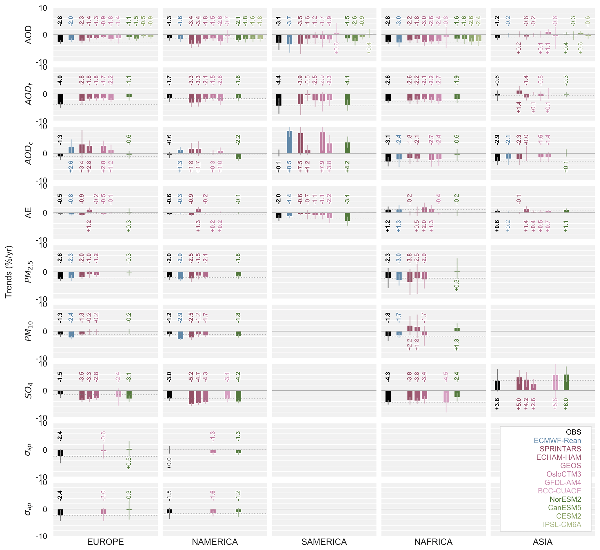
Figure 6Regional trends in the aerosol properties computed with observations and models co-located in space and time with the observations. The error bars correspond to the uncertainty in the trend as calculated using both the uncertainty in the Theil–Sen slope and the residuals. The bold font indicates that the trends are significant at a confidence level of 95 % (p value < 0.05).
This model trends evaluation reveals some key points. First, CAMS-Rean, which assimilates AOD, performs the best for capturing the trends of this parameter. Second, a large intermodel variability is generally found over Asia, where the observed trends are also the most uncertain. Considering the total column, the models usually perform rather well for AOD, AODf and the AE, but they show lower skill for AODc. At the ground level, the models perform well for both SO4 concentration and PM. The trends in σsp and σap computed from regional time series are associated with large uncertainties due to the limited number of stations. This is exacerbated by the fact that data were only available from two models for these parameters.
4.3 Trends in models
4.3.1 Global trends
As discussed previously, the regional trends found are probably not always representative of the trends in the extended regions and over the whole study period. The reason for this is the partial spatial and temporal coverage of the ground-based observations. Moreover, the observation stations are obviously located on land. This does not allow for a depiction of global aerosol trends and is unfortunate as sea salt particles are among the most predominant aerosols on Earth (Schulz et al., 2004).
Unlike observations, models provide data at a global scale and for the entire study period. The completeness of these model datasets offers the opportunity to derive global aerosol trends. In order to provide an assessment of the aerosol trends at a global scale, we present, in this section, the trends computed with NorESM2 (CMIP6 group), which provides data for all of the nine parameters considered in this study. The calculation of the global trend is made by averaging the absolute trends computed at each grid point of the model and using all timestamps in the study period. In order to provide a relative trend, this absolute trend is normalized to the global average of the considered parameter for the year 2000. The global trends are reported for the nine aerosol parameters in Table 4. The global maps, shown in Fig. 7, enable investigation of the spatial variability in these trends.
Table 4Global means and trends of aerosol parameters using NorESM2 model data. The values in parentheses are obtained by aggregating only grid points where observation stations are located while using the complete model time series. The relative trends are calculated by averaging the absolute trends within the considered grid points and normalizing this average to the global mean for the year 2000.
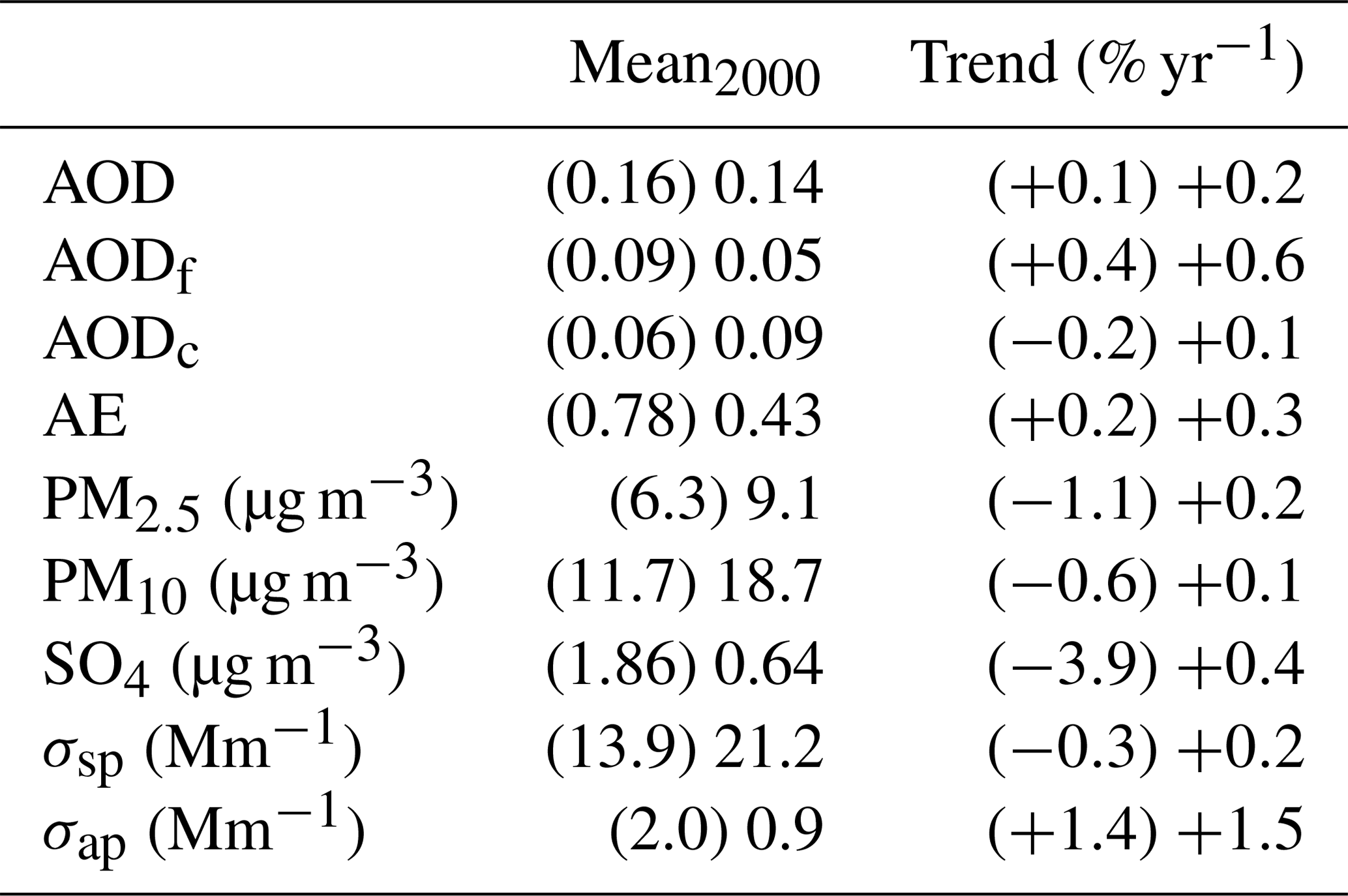
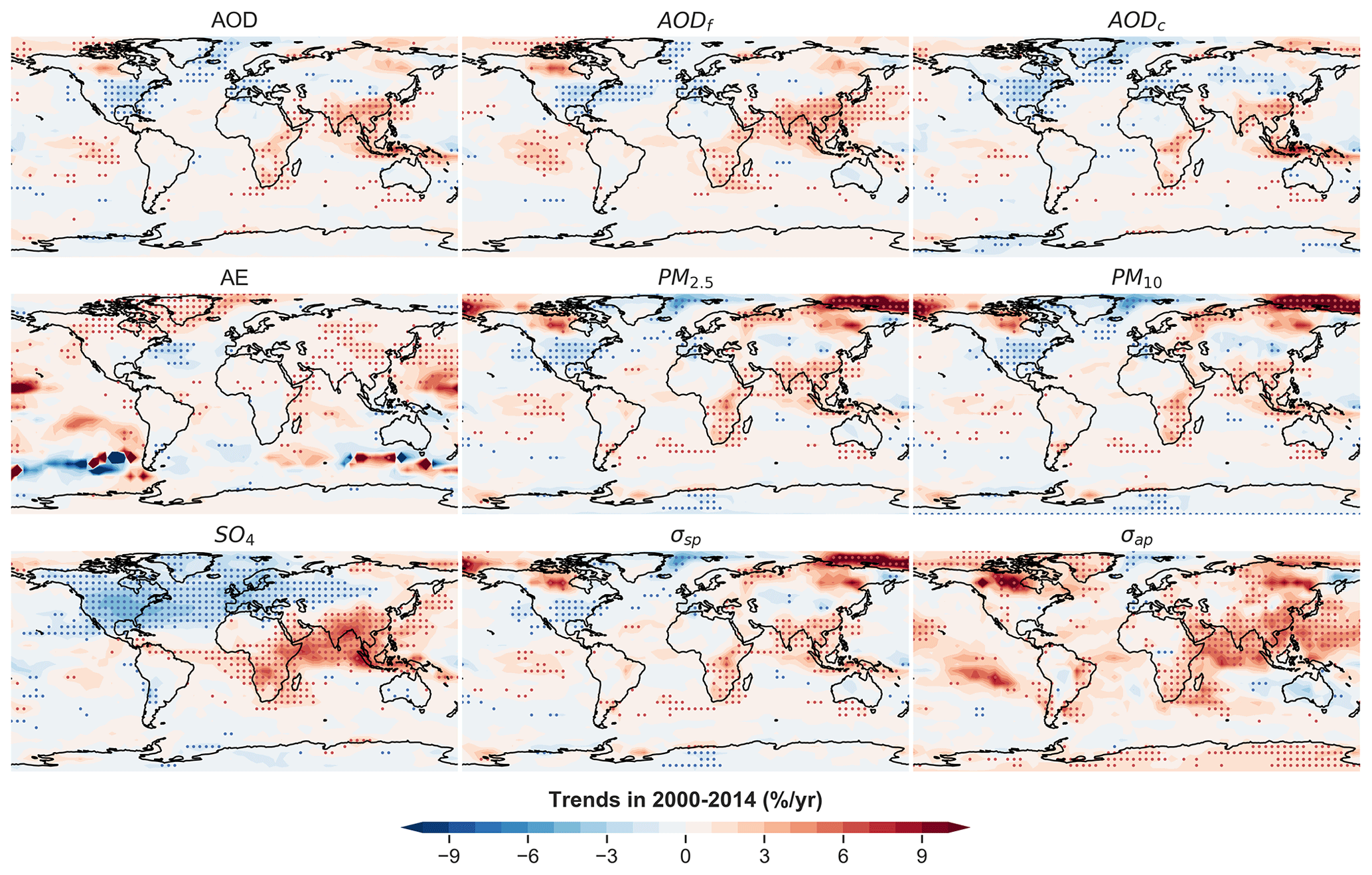
Figure 7Global trends in aerosol properties using NorESM2 data regridded at a 5∘ × 5∘ resolution. The blue and red dots indicate significant negative and positive trends, respectively.
While the observed trends in the three AOD parameters show a decrease in most of the regions of the world, the global AOD trend is actually positive (+0.2 % yr−1). This global increase is also found with other models. Averages of the models from the CAMS-Rean and the AP3 groups simulate global trends of about +0.2 % yr−1 and +0.3 % yr−1, respectively. Within the CMIP6 group, IPSL and CESM2 also exhibit positive trends (+0.7 % yr−1 and +0.3 % yr−1), consistent with NorESM2, while CanESM simulates a negative trend (−0.8 % yr−1). The relative increase of 0.2 % yr−1 found with NorESM2 corresponds to an absolute rate of +0.0028 per decade, which is in excellent agreement with the global trend (over the oceans) of +0.003 per decade reported by Zhang and Reid (2010) using MODIS data. The increase in AOD is observed to be larger for the fine fraction, with an increase of about +0.6 % yr−1, as compared to +0.1 % yr−1 for AODc. As seen in Fig. 7, similar geographical patterns are found for the three AODs: an increase in South Africa and East Asia and decrease in Europe and in the USA. The increasing AOD observed in Canada is dominated by an increase in AODf in this region. The prominent increase in AOD in Indonesia seems to be linked to a large increase in AODc. The tropical Pacific Ocean, off the west coast of South America, has significant positive modeled trends in both AOD and AODf. Almost no significant trend is found south of 60∘ S.
The model also simulates an increase for the AE on a global scale, with a rate of +0.3 % yr−1. This suggests a shift towards smaller particles. The largest increases are found over Canada, Greenland, Siberia and the Pacific Ocean. There are some distinct outliers around 60∘ S. In the Atlantic, we find a decrease in the AE off the east coast of the USA, which is consistent with the decrease in AODf in the same region.
The trends in both PM2.5 and PM10 exhibit similar geographical features to those observed for AOD. In addition, one finds large and significantly increasing trends in the high Arctic that could be explained by a change in the air mass circulation pattern or by the increase in open sea, which might contribute to a higher production of sea salt aerosols (Willis et al., 2018; Abbatt et al., 2019). The global averages show that PM2.5 is increasing faster than PM10 (+0.2 % yr−1 vs. +0.1 % yr−1), which is consistent with the increasing AE, suggesting a relatively higher fraction of fine particles with time.
The surface SO4 concentration trends map reveals two large contrasting regions. Significant decreases are found over North America and Europe, while significant increases are found over southern and eastern Asia and southern to central parts of Africa. This illustrates the shift in polluting activities from the developed countries to the developing countries during the last 2 decades. With an overall increase of +0.4 % yr−1, the global trend is positive.
The σsp trends are very similar to those observed for both PM2.5 and PM10. The same geographical patterns are found, and a similar global average trend amounts to an increase of 0.2 % yr−1 over the study period.
σap reveals increasing tendencies over most of the grid boxes of the model, except in Europe, the eastern part of the USA and Australia. This explains why a large positive global trend is obtained for this parameter, with an average of +1.5 % yr−1. Further analysis shows a good spatial correlation with the black carbon OD (optical depth), which exhibits a strong global positive trend of +2.3 % yr−1, as discussed below.
Table 4 also contains the trends computed for the different aerosol parameters when combining only the grid points where an observation station is located, whether measurements are available or not. Significant differences in so-called global trends can be found when observations are not provided over some regions. This is most obvious for SO4, for which the observation stations are located mostly in Europe and North America and which exhibits decreasing values, while only a few stations are located in the regions associated with increasing values. In this case, the computation of the trends by considering only observation station grid boxes leads to a global decrease of −3.9 % yr−1, while consideration of all of the grid boxes of the model leads to a global increase of +0.4 % yr−1.
4.3.2 Contribution of main aerosol species to the AOD trends
The averaged global trend computed by NorESM2 indicates an increase in AOD in the 2000–2014 period with a rate of about 0.2 % yr−1. The trends in the AE, AODf and AODc indicate that fine-mode particles are primarily responsible for this increase in the atmospheric column.
In this section, we investigate the trends in the major aerosol species simulated by NorESM2. For that purpose, the absolute trends in the individual contribution of these species to the AOD were computed, as well as the trends in the loads and the emissions. The trends in OD and loads are shown in Fig. 8. In this version, NorESM2 simulates a large proportion of sea salt. This is the result of model tuning used for reaching climate equilibrium. While the model attributes too much OD to sea salt (SS), the trends should not be affected by this tuning.

Figure 8Absolute trends in OD and emissions of the main aerosol species computed with NorESM2. The y axis of the trends in OD and the emissions is given according to the power of 10 indicated at the top left corner of each of the subplots.
The relative increase in AOD of +0.2 % yr−1 corresponds to an absolute increase in AOD of yr−1. This positive trend is dominated by an increase in the species-specific ODs of the organic aerosols (OAs), SO4 and black carbon (BC), which are responsible for an increase in the OD of about yr−1, yr−1 and yr−1, respectively. The relative OD trends give a different ranking since the highest increase is found for BC (+2.5 % yr−1), followed by OAs (+0.5 % yr−1). On average, the trends for dust and sea salt OD are slightly negative ( yr−1). Note – these species trends include any associated water which can change as a function of relative humidity.
The trends in OD do not necessarily represent the trends in the aerosol loads, which do not include associated water. The different species have different global mass extinction coefficients (calculated in this study as OD per load; dust – 1.8 m2 g−1, SS – 4.3 m2 g−1, OA – 5.6 m2 g−1, SO4 – 5.3 m2 g−1, BC – 7.6 m2 g−1). For sea salt, opposite trends are observed for the sea salt OD (positive trend) and the sea salt load (negative trend). The analysis of the global maps (not shown in this study) reveals that the largest increases in the sea salt load happen in Indonesia and near the North Pole and result in a relatively larger increase in OD in these areas. These localized increases in sea salt OD drive the global sea salt OD trend and are due, at least in part, to the higher relative humidity at these latitudes which makes the sea salt, which is very hygroscopic, more efficient at light extinction.
The main findings of this multiparameter trend analysis are listed below:
-
The observations exhibit mostly negative trends regarding the extensive parameters in the different regions of the world. Significant decreases are found in Europe, North America, South America, North Africa and Asia. In Asia, the AE increases in time and is consistent with increases in AODf and SO4, which reflects the regional increase in the anthropogenic aerosols in that region in the overall study period from 2000 to 2014.
-
Some observation networks allow for the derivation of representative trends over the whole study period. In other cases, the limited temporal and spatial coverage of the observations can induce artificial and/or highly uncertain trends when using regional time series. Among the 38 computed trends with observation data, 22 are considered as representative of the actual trends occurring in the whole region and study period.
-
The models tend to capture observed AOD, AE, SO4 and PM trends but show larger discrepancies regarding AODc. The smaller number of data available for establishing σsp and σap trends makes the validation of the modeled trends more uncertain.
-
The rather good agreement of the trends across different aerosol parameters between models and observations, when co-locating them in time and space, implies that global model trends, including those in poorly monitored regions, are likely correct.
-
The global trends computed with NorESM2 (CMIP6 group) model data give a different picture than the trends obtained when using only ground-based observations. Global positive trends are found for all of the parameters related to aerosol loading. The trends in AOD are dominated by the increase in the fine particles both in the column and at the surface. This tendency towards finer particles is consistent with the positive trend in the AE. This increase appears to be dominated by organic aerosols, of which the emissions have increased in the study period, and by SO4 aerosols, whose sources were shifted from Europe and North America to Africa and East Asia and for which a global positive SO4 trend is found.
Some elements were not considered in this study, and they could be investigated in order to complete the aerosol trends picture:
-
Some regions are associated with strong seasonal cycles. In South America, the regional time series shows high peaks in AOD, associated with forest fires in the late summer, whose intensity greatly varies from year to year. In Africa, a strong seasonal contrast is also found due to the transport of desert dust at altitude in the summer months (Mortier et al., 2016; Ogunjobi et al., 2008). The computation of the seasonal trends would allow characterization of the tendencies in such extreme or synoptic aerosol events.
-
This study shows that the trends computed from the ground-based observation networks are not representative of the global aerosol trends due to the inhomogeneities in data spatial coverage. The satellites providing a global Earth observation could be utilized for the evaluation of the model trends in the regions lacking observations and over the oceans (Hsu et al., 2012; Zhang and Reid, 2010).
-
The trends in the meteorological parameters could be investigated in parallel with the aerosol trends because they affect the aerosol life cycle and their optical properties (Che et al., 2019). Hypothetical trends in wind velocity could produce trends in the loads of sea salt and dust and, as seen in the last section, trends in OD could also be enhanced by relative humidity changes. Changes in temperature could impact the magnitude of the biogenic emissions. Indeed, increasing temperatures, associated with changes in land use and high atmospheric CO2 concentrations, have been shown to lead to an increase in the VOC emissions (Peñuelas and Staudt, 2010). Finally, trends in precipitation that are responsible for aerosol wet scavenging would directly impact trends in aerosol loads.
-
Several studies have linked the trends in anthropogenic aerosols to radiative-forcing variations while investigating sources of global dimming and brightening (Streets et al., 2006; Norris and Wild, 2007). It could be of interest to evaluate how much the modeled trend deviations, as compared to the observations, are affecting the calculation of the radiative forcing, in the different regions of the world and at a global scale.
-
While the mountain sites were excluded from this study, it could be of interest to investigate the trends at higher altitude (which may be related to changes in long-range transport) by including the in situ and remote sensing stations higher than 1000 m (Jungfraujoch, Mauna Loa Observatory, etc.). Similarly, it may also be of interest to look at trends in smaller regions (e.g., split North America into several subregions which are more internally consistent in terms of climate and environment than the large North America region defined here or consider southern Europe as its own region rather than combining it with the North Africa region as was done here).
The observation and model data were read and co-located with the pyaerocom Python library, developed by MET Norway (https://doi.org/10.5281/zenodo.4139879, version 0.9.1) (Gliß et al., 2020b).
The supplement related to this article is available online at: https://doi.org/10.5194/acp-20-13355-2020-supplement.
AM coordinated the study, was responsible for the statistical calculation and analysis, and wrote the paper. JG is the main developer of the pyaerocom library. MS provided feedback on the methods and the manuscript. WA, EA, JH and PL provided in situ data, contributed to the writing of the observation dataset section and provided feedback on the manuscript. BH is the principal investigator of AERONET. HB, MC, PG, HZ, ZK, AK, TL, GM, DN, DO, KvS, TT, RBS and ST provided model output data and feedback on the manuscript.
The authors declare that they have no conflict of interest.
This article is part of the special issue “The Aerosol Chemistry Model Intercomparison Project (AerChemMIP)”. It is not associated with a conference.
Data providers from all the regional and global networks are greatly acknowledged for sharing and submitting their data to be used. The ECHAM-HAMMOZ model is developed by a consortium composed of ETH Zurich, Max Planck Institut für Meteorologie, Forschungszentrum Jülich, University of Oxford, the Finnish Meteorological Institute and the Leibniz Institute for Tropospheric Research and is managed by the Center for Climate Systems Modeling (C2SM) at ETH Zurich. Computing and data storage resources, including the Cheyenne supercomputer (https://doi.org/10.5065/D6RX99HX), were provided by the Computational and Information Systems Laboratory (CISL) at NCAR. All simulations were carried out on the Cheyenne high-performance computing platform https://www2.cisl.ucar.edu/user-support/acknowledging-ncarcisl (last access: 20 November 2020), and are available to the community via the Earth System Grid. High-performance computing and storage resources were provided by MET and the Norwegian infrastructure for computational science (through projects NN2345K, NN9252K, NS2345K and NS9252K).
This research has been supported by the European Commission, H2020 Research Infrastructures (FORCeS (grant no. 821205), CRESCENDO (Coordinated Research in Earth Systems and Climate: Experiments, Knowledge, Dissemination and Outreach; grant no. 641816)), the National Science Foundation (NSF; grant no. 1852977), the Research Council of Norway (grant no. 295046) and the Copernicus Atmospheric Monitoring Service (grant no. CAMS84).
This paper was edited by Pedro Jimenez-Guerrero and reviewed by two anonymous referees.
Aas, W., Mortier, A., Bowersox, V., Cherian, R., Faluvegi, G., Fagerli, H., Hand, J., Klimont, Z., Galy-Lacaux, C., Lehmann, C. M., and Myhre, C. L.: Global and regional trends of atmospheric sulfur, Sci. Rep., 9, 953, https://doi.org/10.1038/s41598-018-37304-0, 2019. a, b, c, d, e, f, g, h
Abbatt, J. P. D., Leaitch, W. R., Aliabadi, A. A., Bertram, A. K., Blanchet, J.-P., Boivin-Rioux, A., Bozem, H., Burkart, J., Chang, R. Y. W., Charette, J., Chaubey, J. P., Christensen, R. J., Cirisan, A., Collins, D. B., Croft, B., Dionne, J., Evans, G. J., Fletcher, C. G., Galí, M., Ghahremaninezhad, R., Girard, E., Gong, W., Gosselin, M., Gourdal, M., Hanna, S. J., Hayashida, H., Herber, A. B., Hesaraki, S., Hoor, P., Huang, L., Hussherr, R., Irish, V. E., Keita, S. A., Kodros, J. K., Köllner, F., Kolonjari, F., Kunkel, D., Ladino, L. A., Law, K., Levasseur, M., Libois, Q., Liggio, J., Lizotte, M., Macdonald, K. M., Mahmood, R., Martin, R. V., Mason, R. H., Miller, L. A., Moravek, A., Mortenson, E., Mungall, E. L., Murphy, J. G., Namazi, M., Norman, A.-L., O'Neill, N. T., Pierce, J. R., Russell, L. M., Schneider, J., Schulz, H., Sharma, S., Si, M., Staebler, R. M., Steiner, N. S., Thomas, J. L., von Salzen, K., Wentzell, J. J. B., Willis, M. D., Wentworth, G. R., Xu, J.-W., and Yakobi-Hancock, J. D.: Overview paper: New insights into aerosol and climate in the Arctic, Atmos. Chem. Phys., 19, 2527–2560, https://doi.org/10.5194/acp-19-2527-2019, 2019. a
Aragão, L. E., Anderson, L. O., Fonseca, M. G., Rosan, T. M., Vedovato, L. B., Wagner, F. H., Silva, C. V., Junior, C. H. S., Arai, E., Aguiar, A. P., and Barlow, J.: 21st Century drought-related fires counteract the decline of Amazon deforestation carbon emissions, Nat. Commun., 9, 536, https://doi.org/10.1038/s41467-017-02771-y, 2018. a
Barreto, Á., Cuevas, E., Granados-Muñoz, M.-J., Alados-Arboledas, L., Romero, P. M., Gröbner, J., Kouremeti, N., Almansa, A. F., Stone, T., Toledano, C., Román, R., Sorokin, M., Holben, B., Canini, M., and Yela, M.: The new sun-sky-lunar Cimel CE318-T multiband photometer – a comprehensive performance evaluation, Atmos. Meas. Tech., 9, 631–654, https://doi.org/10.5194/amt-9-631-2016, 2016. a
Bauer, S. E. and Koch, D.: Impact of heterogeneous sulfate formation at mineral dust surfaces on aerosol loads and radiative forcing in the Goddard Institute for Space Studies general circulation model, J. Geophys. Res.-Atmos., 110, D17202, https://doi.org/10.1029/2005JD005870, 2005. a
Bauer, S. E., Mishchenko, M. I., Lacis, A. A., Zhang, S., Perlwitz, J., and Metzger, S. M.: Do sulfate and nitrate coatings on mineral dust have important effects on radiative properties and climate modeling?, J. Geophys. Res.-Atmos., 112, D06307, https://doi.org/10.1029/2005JD006977, 2007. a
Bell, M. L., Davis, D. L., and Fletcher, T.: A retrospective assessment of mortality from the London smog episode of 1952: the role of influenza and pollution, Environ. Health Persp., 112, 6–8, https://doi.org/10.1289/ehp.6539, 2004. a
Betts, R., Sanderson, M., and Woodward, S.: Effects of large-scale Amazon forest degradation on climate and air quality through fluxes of carbon dioxide, water, energy, mineral dust and isoprene, Philos. T. R. Soc. B, 363, 1873–1880, https://doi.org/10.1098/rstb.2007.0027, 2008. a
Bian, H., Chin, M., Hauglustaine, D. A., Schulz, M., Myhre, G., Bauer, S. E., Lund, M. T., Karydis, V. A., Kucsera, T. L., Pan, X., Pozzer, A., Skeie, R. B., Steenrod, S. D., Sudo, K., Tsigaridis, K., Tsimpidi, A. P., and Tsyro, S. G.: Investigation of global particulate nitrate from the AeroCom phase III experiment, Atmos. Chem. Phys., 17, 12911–12940, https://doi.org/10.5194/acp-17-12911-2017, 2017. a
Bryner, G. C.: Blue skies, green politics: The clean air act of 1990, Congressional Quarterly Press, Washington, DC, USA, 1995. a
Burnett, R. T., Pope III, C. A., Ezzati, M., Olives, C., Lim, S. S., Mehta, S., Shin, H. H., Singh, G., Hubbell, B., Brauer, M., and Anderson, H. R.: An integrated risk function for estimating the global burden of disease attributable to ambient fine particulate matter exposure, Environ. Health Persp., 122, 397–403, https://doi.org/10.1289/ehp.1307049, 2014. a
Che, H., Gui, K., Xia, X., Wang, Y., Holben, B. N., Goloub, P., Cuevas-Agulló, E., Wang, H., Zheng, Y., Zhao, H., and Zhang, X.: Large contribution of meteorological factors to inter-decadal changes in regional aerosol optical depth, Atmos. Chem. Phys., 19, 10497–10523, https://doi.org/10.5194/acp-19-10497-2019, 2019. a
Chin, M., Ginoux, P., Kinne, S., Torres, O., Holben, B. N., Duncan, B. N., Martin, R. V., Logan, J. A., Higurashi, A., and Nakajima, T.: Tropospheric aerosol optical thickness from the GOCART model and comparisons with satellite and Sun photometer measurements, J. Atmos. Sci., 59, 461–483, https://doi.org/10.1175/1520-0469(2002)059<0461:TAOTFT>2.0.CO;2, 2002. a
Chin, M., Diehl, T., Tan, Q., Prospero, J. M., Kahn, R. A., Remer, L. A., Yu, H., Sayer, A. M., Bian, H., Geogdzhayev, I. V., Holben, B. N., Howell, S. G., Huebert, B. J., Hsu, N. C., Kim, D., Kucsera, T. L., Levy, R. C., Mishchenko, M. I., Pan, X., Quinn, P. K., Schuster, G. L., Streets, D. G., Strode, S. A., Torres, O., and Zhao, X.-P.: Multi-decadal aerosol variations from 1980 to 2009: a perspective from observations and a global model, Atmos. Chem. Phys., 14, 3657–3690, https://doi.org/10.5194/acp-14-3657-2014, 2014. a
Collaud Coen, M., Andrews, E., Alastuey, A., Arsov, T. P., Backman, J., Brem, B. T., Bukowiecki, N., Couret, C., Eleftheriadis, K., Flentje, H., Fiebig, M., Gysel-Beer, M., Hand, J. L., Hoffer, A., Hooda, R., Hueglin, C., Joubert, W., Keywood, M., Kim, J. E., Kim, S.-W., Labuschagne, C., Lin, N.-H., Lin, Y., Lund Myhre, C., Luoma, K., Lyamani, H., Marinoni, A., Mayol-Bracero, O. L., Mihalopoulos, N., Pandolfi, M., Prats, N., Prenni, A. J., Putaud, J.-P., Ries, L., Reisen, F., Sellegri, K., Sharma, S., Sheridan, P., Sherman, J. P., Sun, J., Titos, G., Torres, E., Tuch, T., Weller, R., Wiedensohler, A., Zieger, P., and Laj, P.: Multidecadal trend analysis of in situ aerosol radiative properties around the world, Atmos. Chem. Phys., 20, 8867–8908, https://doi.org/10.5194/acp-20-8867-2020, 2020. a, b, c, d, e
Colarco, P., da Silva, A., Chin, M., and Diehl, T.: Online simulations of global aerosol distributions in the NASA GEOS-4 model and comparisons to satellite and ground-based aerosol optical depth, J. Geophys. Res.-Atmos., 115, D14207, https://doi.org/10.1029/2009JD012820, 2010. a
Danabasoglu, G., Lamarque, J. F., Bacmeister, J., Bailey, D. A., DuVivier, A. K., Edwards, J., Emmons, L. K., Fasullo, J., Garcia, R., Gettelman, A., and Hannay, C.: The Community Earth System Model version 2 (CESM2), J. Adv. Model. Earth Sy., 12, e2019MS001916, https://doi.org/10.1029/2019MS001916, 2020. a
de Meij, A., Pozzer, A., and Lelieveld, J.: Trend analysis in aerosol optical depths and pollutant emission estimates between 2000 and 2009, Atmos. Environ., 51, 75–85, https://doi.org/10.1016/j.atmosenv.2012.01.059, 2012. a
Eyring, V., Bony, S., Meehl, G. A., Senior, C. A., Stevens, B., Stouffer, R. J., and Taylor, K. E.: Overview of the Coupled Model Intercomparison Project Phase 6 (CMIP6) experimental design and organization, Geosci. Model Dev., 9, 1937–1958, https://doi.org/10.5194/gmd-9-1937-2016, 2016. a
Fan, S.-M., Horowitz, L. W., Levy, H., and Moxim, W. J.: Impact of air pollution on wet deposition of mineral dust aerosols, Geophys. Res. Lett., 31, L02104, https://doi.org/10.1029/2003GL018501, 2004. a
Giles, D. M., Sinyuk, A., Sorokin, M. G., Schafer, J. S., Smirnov, A., Slutsker, I., Eck, T. F., Holben, B. N., Lewis, J. R., Campbell, J. R., Welton, E. J., Korkin, S. V., and Lyapustin, A. I.: Advancements in the Aerosol Robotic Network (AERONET) Version 3 database – automated near-real-time quality control algorithm with improved cloud screening for Sun photometer aerosol optical depth (AOD) measurements, Atmos. Meas. Tech., 12, 169–209, https://doi.org/10.5194/amt-12-169-2019, 2019. a
Glantz, P., Freud, E., Johansson, C., Noone, K. J., and Tesche, M.: Trends in MODIS and AERONET derived aerosol optical thickness over Northern Europe, Tellus B: Chemical and Physical Meteorology, 71, 1–20, https://doi.org/10.1080/16000889.2018.1554414, 2019. a
Gliß, J., Mortier, A., Schulz, M., Andrews, E., Balkanski, Y., Bauer, S. E., Benedictow, A. M. K., Bian, H., Checa-Garcia, R., Chin, M., Ginoux, P., Griesfeller, J. J., Heckel, A., Kipling, Z., Kirkevåg, A., Kokkola, H., Laj, P., Le Sager, P., Lund, M. T., Lund Myhre, C., Matsui, H., Myhre, G., Neubauer, D., van Noije, T., North, P., Olivié, D. J. L., Sogacheva, L., Takemura, T., Tsigaridis, K., and Tsyro, S. G.: Multi-model evaluation of aerosol optical properties in the AeroCom phase III Control experiment, using ground and space based columnar observations from AERONET, MODIS, AATSR and a merged satellite product as well as surface in-situ observations from GAW sites, Atmos. Chem. Phys. Discuss., https://doi.org/10.5194/acp-2019-1214, in review, 2020a. a, b, c
Gliß, J., Griesfeller, J., Schulz, M., and the pyaerocom developer team: metno/pyaerocom: Version used in Mortier et al., ACP, 2020 (Version v0.9.1), Zenodo, https://doi.org/10.5281/zenodo.4139879, 2020b. a
Hamed, K. H. and Rao, A. R.: A modified Mann-Kendall trend test for autocorrelated data, J. Hydrol., 204, 182–196, https://doi.org/10.1016/S0022-1694(97)00125-X, 1998. a
Hand, J., Gill, T., and Schichtel, B.: Urban and rural coarse aerosol mass across the United States: Spatial and seasonal variability and long-term trends, Atmos. Environ., 218, 117025, https://doi.org/10.1016/j.atmosenv.2019.117025, 2019a. a, b
Hand, J., Prenni, A., Schichtel, B., Malm, W., and Chow, J.: Trends in remote PM2.5 residual mass across the United States: Implications for aerosol mass reconstruction in the IMPROVE network, Atmos. Environ., 203, 141–152, https://doi.org/10.1016/j.atmosenv.2019.01.049, 2019b. a, b
Haywood, J. and Boucher, O.: Estimates of the direct and indirect radiative forcing due to tropospheric aerosols: A review, Rev. Geophys., 38, 513–543, https://doi.org/10.1029/1999RG000078, 2000. a
Holben, B. N., Tanre, D., Smirnov, A., Eck, T. F., Slutsker, I., Abuhassan, N., Newcomb, W. W., Schafer, J. S., Chatenet, B., Lavenu, F., and Kaufman, Y. J.: An emerging ground-based aerosol climatology: Aerosol optical depth from AERONET, J. Geophys. Res.-Atmos., 106, 12067–12097, https://doi.org/10.1029/2001JD900014, 2001. a, b, c, d
Hsu, N. C., Gautam, R., Sayer, A. M., Bettenhausen, C., Li, C., Jeong, M. J., Tsay, S.-C., and Holben, B. N.: Global and regional trends of aerosol optical depth over land and ocean using SeaWiFS measurements from 1997 to 2010, Atmos. Chem. Phys., 12, 8037–8053, https://doi.org/10.5194/acp-12-8037-2012, 2012. a
Huneeus, N., Schulz, M., Balkanski, Y., Griesfeller, J., Prospero, J., Kinne, S., Bauer, S., Boucher, O., Chin, M., Dentener, F., Diehl, T., Easter, R., Fillmore, D., Ghan, S., Ginoux, P., Grini, A., Horowitz, L., Koch, D., Krol, M. C., Landing, W., Liu, X., Mahowald, N., Miller, R., Morcrette, J.-J., Myhre, G., Penner, J., Perlwitz, J., Stier, P., Takemura, T., and Zender, C. S.: Global dust model intercomparison in AeroCom phase I, Atmos. Chem. Phys., 11, 7781–7816, https://doi.org/10.5194/acp-11-7781-2011, 2011. a
Inness, A., Ades, M., Agustí-Panareda, A., Barré, J., Benedictow, A., Blechschmidt, A.-M., Dominguez, J. J., Engelen, R., Eskes, H., Flemming, J., Huijnen, V., Jones, L., Kipling, Z., Massart, S., Parrington, M., Peuch, V.-H., Razinger, M., Remy, S., Schulz, M., and Suttie, M.: The CAMS reanalysis of atmospheric composition, Atmos. Chem. Phys., 19, 3515–3556, https://doi.org/10.5194/acp-19-3515-2019, 2019. a, b, c
Johnson, B., Shine, K., and Forster, P.: The semi-direct aerosol effect: Impact of absorbing aerosols on marine stratocumulus, Q. J. Roy. Meteor. Soc., 130, 1407–1422, https://doi.org/10.1256/qj.03.61, 2004. a
Kaufman, Y. J., Tanré, D., and Boucher, O.: A satellite view of aerosols in the climate system, Nature, 419, 215–223, https://doi.org/10.1038/nature01091, 2002. a
Kinne, S., Schulz, M., Textor, C., Guibert, S., Balkanski, Y., Bauer, S. E., Berntsen, T., Berglen, T. F., Boucher, O., Chin, M., Collins, W., Dentener, F., Diehl, T., Easter, R., Feichter, J., Fillmore, D., Ghan, S., Ginoux, P., Gong, S., Grini, A., Hendricks, J., Herzog, M., Horowitz, L., Isaksen, I., Iversen, T., Kirkevåg, A., Kloster, S., Koch, D., Kristjansson, J. E., Krol, M., Lauer, A., Lamarque, J. F., Lesins, G., Liu, X., Lohmann, U., Montanaro, V., Myhre, G., Penner, J., Pitari, G., Reddy, S., Seland, O., Stier, P., Takemura, T., and Tie, X.: An AeroCom initial assessment – optical properties in aerosol component modules of global models, Atmos. Chem. Phys., 6, 1815–1834, https://doi.org/10.5194/acp-6-1815-2006, 2006. a
Kinne, S., O'Donnel, D., Stier, P., Kloster, S., Zhang, K., Schmidt, H., Rast, S., Giorgetta, M., Eck, T. F., and Stevens, B.: MAC-v1: A new global aerosol climatology for climate studies, J. Adv. Model. Earth Sy., 5, 704–740, https://doi.org/10.1029/2002JD002975, 2013. a
Kirkevåg, A., Grini, A., Olivié, D., Seland, Ø., Alterskjær, K., Hummel, M., Karset, I. H. H., Lewinschal, A., Liu, X., Makkonen, R., Bethke, I., Griesfeller, J., Schulz, M., and Iversen, T.: A production-tagged aerosol module for Earth system models, OsloAero5.3 – extensions and updates for CAM5.3-Oslo, Geosci. Model Dev., 11, 3945–3982, https://doi.org/10.5194/gmd-11-3945-2018, 2018. a
Labordena, M., Neubauer, D., Folini, D., Patt, A., and Lilliestam, J.: Blue skies over China: The effect of pollution-control on solar power generation and revenues, PloS One, 13, e0207028, https://doi.org/10.1371/journal.pone.0207028, 2018. a
Laj, P., Bigi, A., Rose, C., Andrews, E., Lund Myhre, C., Collaud Coen, M., Lin, Y., Wiedensohler, A., Schulz, M., Ogren, J. A., Fiebig, M., Gliß, J., Mortier, A., Pandolfi, M., Petäja, T., Kim, S.-W., Aas, W., Putaud, J.-P., Mayol-Bracero, O., Keywood, M., Labrador, L., Aalto, P., Ahlberg, E., Alados Arboledas, L., Alastuey, A., Andrade, M., Artíñano, B., Ausmeel, S., Arsov, T., Asmi, E., Backman, J., Baltensperger, U., Bastian, S., Bath, O., Beukes, J. P., Brem, B. T., Bukowiecki, N., Conil, S., Couret, C., Day, D., Dayantolis, W., Degorska, A., Eleftheriadis, K., Fetfatzis, P., Favez, O., Flentje, H., Gini, M. I., Gregorič, A., Gysel-Beer, M., Hallar, A. G., Hand, J., Hoffer, A., Hueglin, C., Hooda, R. K., Hyvärinen, A., Kalapov, I., Kalivitis, N., Kasper-Giebl, A., Kim, J. E., Kouvarakis, G., Kranjc, I., Krejci, R., Kulmala, M., Labuschagne, C., Lee, H.-J., Lihavainen, H., Lin, N.-H., Löschau, G., Luoma, K., Marinoni, A., Martins Dos Santos, S., Meinhardt, F., Merkel, M., Metzger, J.-M., Mihalopoulos, N., Nguyen, N. A., Ondracek, J., Pérez, N., Perrone, M. R., Petit, J.-E., Picard, D., Pichon, J.-M., Pont, V., Prats, N., Prenni, A., Reisen, F., Romano, S., Sellegri, K., Sharma, S., Schauer, G., Sheridan, P., Sherman, J. P., Schütze, M., Schwerin, A., Sohmer, R., Sorribas, M., Steinbacher, M., Sun, J., Titos, G., Toczko, B., Tuch, T., Tulet, P., Tunved, P., Vakkari, V., Velarde, F., Velasquez, P., Villani, P., Vratolis, S., Wang, S.-H., Weinhold, K., Weller, R., Yela, M., Yus-Diez, J., Zdimal, V., Zieger, P., and Zikova, N.: A global analysis of climate-relevant aerosol properties retrieved from the network of Global Atmosphere Watch (GAW) near-surface observatories, Atmos. Meas. Tech., 13, 4353–4392, https://doi.org/10.5194/amt-13-4353-2020, 2020. a, b
Li, X., Wagner, F., Peng, W., Yang, J., and Mauzerall, D. L.: Reduction of solar photovoltaic resources due to air pollution in China, P. Natl. Acad. Sci., 114, 11867–11872, https://doi.org/10.1073/pnas.1711462114, 2017. a
Likens, G. E., Butler, T. J., and Buso, D. C.: Long-and short-term changes in sulfate deposition: effects of the 1990 Clean Air Act Amendments, Biogeochemistry, 52, 1–11, https://doi.org/10.1023/A:1026563400336, 2001. a
Lohmann, U. and Feichter, J.: Global indirect aerosol effects: a review, Atmos. Chem. Phys., 5, 715–737, https://doi.org/10.5194/acp-5-715-2005, 2005. a
Lund, M. T., Myhre, G., Haslerud, A. S., Skeie, R. B., Griesfeller, J., Platt, S. M., Kumar, R., Myhre, C. L., and Schulz, M.: Concentrations and radiative forcing of anthropogenic aerosols from 1750 to 2014 simulated with the Oslo CTM3 and CEDS emission inventory, Geosci. Model Dev., 11, 4909–4931, https://doi.org/10.5194/gmd-11-4909-2018, 2018. a
Lurton, T., Balkanski, Y., Bastrikov, V., Bekki, S., Bopp, L., Braconnot, P., Brockmann, P., Cadule, P., Contoux, C., Cozic, A., and Cugnet, D.: Implementation of the CMIP6 forcing data in the IPSL-CM6A-LR model, J. Adv. Model. Earth Sy., https://doi.org/10.1029/2019MS001940, 2019. a
Mortier, A., Goloub, P., Derimian, Y., Tanré, D., Podvin, T., Blarel, L., Deroo, C., Marticorena, B., Diallo, A., and Ndiaye, T.: Climatology of aerosol properties and clear-sky shortwave radiative effects using Lidar and Sun photometer observations in the Dakar site, J. Geophys. Res.-Atmos., 121, 6489–6510, https://doi.org/10.1002/2015JD024588, 2016. a
Myhre, G., Berglen, T. F., Johnsrud, M., Hoyle, C. R., Berntsen, T. K., Christopher, S. A., Fahey, D. W., Isaksen, I. S. A., Jones, T. A., Kahn, R. A., Loeb, N., Quinn, P., Remer, L., Schwarz, J. P., and Yttri, K. E.: Modelled radiative forcing of the direct aerosol effect with multi-observation evaluation, Atmos. Chem. Phys., 9, 1365–1392, https://doi.org/10.5194/acp-9-1365-2009, 2009. a
Neubauer, D., Ferrachat, S., Siegenthaler-Le Drian, C., Stier, P., Partridge, D. G., Tegen, I., Bey, I., Stanelle, T., Kokkola, H., and Lohmann, U.: The global aerosol–climate model ECHAM6.3–HAM2.3 – Part 2: Cloud evaluation, aerosol radiative forcing, and climate sensitivity, Geosci. Model Dev., 12, 3609–3639, https://doi.org/10.5194/gmd-12-3609-2019, 2019. a, b
Norris, J. R. and Wild, M.: Trends in aerosol radiative effects over Europe inferred from observed cloud cover, solar “dimming,” and solar “brightening”, J. Geophys. Res.-Atmos., 112, D08214, https://doi.org/10.1029/2006JD007794, 2007. a
Ogunjobi, K., Ajayi, V., Balogun, I., Omotosho, J., and He, Z.: The synoptic and optical characteristics of the harmattan dust spells over Nigeria, Theor. Appl. Climatol., 93, 91–105, https://doi.org/10.1007/s00704-007-0332-2, 2008. a
O'Neill, N., Eck, T., Smirnov, A., Holben, B., and Thulasiraman, S.: Spectral discrimination of coarse and fine mode optical depth, J. Geophys. Res.-Atmos., 108, 4559, https://doi.org/10.1029/2002JD002975, 2003. a
Pandolfi, M., Alados-Arboledas, L., Alastuey, A., Andrade, M., Angelov, C., Artiñano, B., Backman, J., Baltensperger, U., Bonasoni, P., Bukowiecki, N., Collaud Coen, M., Conil, S., Coz, E., Crenn, V., Dudoitis, V., Ealo, M., Eleftheriadis, K., Favez, O., Fetfatzis, P., Fiebig, M., Flentje, H., Ginot, P., Gysel, M., Henzing, B., Hoffer, A., Holubova Smejkalova, A., Kalapov, I., Kalivitis, N., Kouvarakis, G., Kristensson, A., Kulmala, M., Lihavainen, H., Lunder, C., Luoma, K., Lyamani, H., Marinoni, A., Mihalopoulos, N., Moerman, M., Nicolas, J., O'Dowd, C., Petäjä, T., Petit, J.-E., Pichon, J. M., Prokopciuk, N., Putaud, J.-P., Rodríguez, S., Sciare, J., Sellegri, K., Swietlicki, E., Titos, G., Tuch, T., Tunved, P., Ulevicius, V., Vaishya, A., Vana, M., Virkkula, A., Vratolis, S., Weingartner, E., Wiedensohler, A., and Laj, P.: A European aerosol phenomenology – 6: scattering properties of atmospheric aerosol particles from 28 ACTRIS sites, Atmos. Chem. Phys., 18, 7877–7911, https://doi.org/10.5194/acp-18-7877-2018, 2018. a
Peñuelas, J. and Staudt, M.: BVOCs and global change, Trends Plant Sci., 15, 133–144, https://doi.org/10.1016/j.tplants.2009.12.005, 2010. a
Pöschl, U.: Atmospheric aerosols: composition, transformation, climate and health effects, Angew. Chem. Int. Edit., 44, 7520–7540, https://doi.org/10.1002/anie.200501122, 2005. a
Putaud, J.-P., Dingenen, R. V., Alastuey, A., Bauer, H., Birmili, W., Cyrys, J., Flentje, H., Fuzzi, S., Gehrig, R., Hansson, H., Harrison, R., Herrmann, H., Hitzenberger, R., Hüglin, C., Jones, A., Kasper-Giebl, A., Kiss, G., Kousa, A., Kuhlbusch, T., Löschau, G., Maenhaut, W., Molnar, A., Moreno, T., Pekkanen, J., Perrino, C., Pitz, M., Puxbaum, H., Querol, X., Rodriguez, S., Salma, I., Schwarz, J., Smolik, J., Schneider, J., Spindler, G., ten Brink, H., Tursic, J., Viana, M., Wiedensohler, A., and Raes, F.: A European aerosol phenomenology – 3: Physical and chemical characteristics of particulate matter from 60 rural, urban, and kerbside sites across Europe, Atmos. Environ., 44, 1308–1320, https://doi.org/10.1016/j.atmosenv.2009.12.011, 2010. a
Ramachandran, S., Kedia, S., and Srivastava, R.: Aerosol optical depth trends over different regions of India, Atmos. Environ., 49, 338–347, https://doi.org/10.1016/j.atmosenv.2011.11.017, 2012. a
Rap, A., Scott, C. E., Spracklen, D. V., Bellouin, N., Forster, P. M., Carslaw, K. S., Schmidt, A., and Mann, G.: Natural aerosol direct and indirect radiative effects, Geophys. Res. Lett., 40, 3297–3301, https://doi.org/10.1002/grl.50441, 2013. a
Schulz, M., de Leeuw, G., and Balkanski, Y.: Sea-salt aerosol source functions and emissions, in: Emissions of Atmospheric Trace Compounds, edited by: Granier, C., Artaxo, P., and Reeves, C. E., Springer, Dordrecht, 333–359, https://doi.org/10.1007/978-1-4020-2167-1_9, 2004. a
Schulz, M., Textor, C., Kinne, S., Balkanski, Y., Bauer, S., Berntsen, T., Berglen, T., Boucher, O., Dentener, F., Guibert, S., Isaksen, I. S. A., Iversen, T., Koch, D., Kirkevåg, A., Liu, X., Montanaro, V., Myhre, G., Penner, J. E., Pitari, G., Reddy, S., Seland, Ø., Stier, P., and Takemura, T.: Radiative forcing by aerosols as derived from the AeroCom present-day and pre-industrial simulations, Atmos. Chem. Phys., 6, 5225–5246, https://doi.org/10.5194/acp-6-5225-2006, 2006. a
Schutgens, N., Tsyro, S., Gryspeerdt, E., Goto, D., Weigum, N., Schulz, M., and Stier, P.: On the spatio-temporal representativeness of observations, Atmos. Chem. Phys., 17, 9761–9780, https://doi.org/10.5194/acp-17-9761-2017, 2017. a
Schutgens, N. A. J.: Site representativity of AERONET and GAW remotely sensed aerosol optical thickness and absorbing aerosol optical thickness observations, Atmos. Chem. Phys., 20, 7473–7488, https://doi.org/10.5194/acp-20-7473-2020, 2020. a
Seland, Ø., Bentsen, M., Seland Graff, L., Olivié, D., Toniazzo, T., Gjermundsen, A., Debernard, J. B., Gupta, A. K., He, Y., Kirkevåg, A., Schwinger, J., Tjiputra, J., Schancke Aas, K., Bethke, I., Fan, Y., Griesfeller, J., Grini, A., Guo, C., Ilicak, M., Hafsahl Karset, I. H., Landgren, O., Liakka, J., Onsum Moseid, K., Nummelin, A., Spensberger, C., Tang, H., Zhang, Z., Heinze, C., Iverson, T., and Schulz, M.: The Norwegian Earth System Model, NorESM2 – Evaluation of theCMIP6 DECK and historical simulations, Geosci. Model Dev. Discuss., https://doi.org/10.5194/gmd-2019-378, in review, 2020. a
Sen, P. K.: Estimates of the regression coefficient based on Kendall's tau, J. Am. Stat. Assoc., 63, 1379–1389, https://doi.org/10.1080/01621459.1968.10480934, 1968. a
Smirnov, A., Holben, B., Eck, T., Dubovik, O., and Slutsker, I.: Cloud-screening and quality control algorithms for the AERONET database, Remote Sens. Environ., 73, 337–349, https://doi.org/10.1016/S0034-4257(00)00109-7, 2000. a
Smirnov, A., Holben, B., Lyapustin, A., Slutsker, I., and Eck, T.: AERONET processing algorithms refinement, in: AERONET Workshop, El Arenosillo, Spain, 10–14 May 2004, pp. 10–14, 2004. a
Stocker, T. F., Qin, D., Plattner, G.-K., Tignor, M., Allen, S. K., Boschung, J., Nauels, A., Xia, Y., Bex, V., and Midgley, P. M.: Climate Change 2013: The Physical Science Basis. Contribution of Working Group I to the Fifth Assessment Report of the Intergovernmental Panel on Climate Change, Cambridge University Press, New York, NY, USA, 1535 pp., 2014. a
Streets, D. G., Wu, Y., and Chin, M.: Two-decadal aerosol trends as a likely explanation of the global dimming/brightening transition, Geophys. Res. Lett., 33, L15806, https://doi.org/10.1029/2006GL026471, 2006. a
Streets, D. G., Yu, C., Wu, Y., Chin, M., Zhao, Z., Hayasaka, T., and Shi, G.: Aerosol trends over China, 1980–2000, Atmos. Res., 88, 174–182, https://doi.org/10.1016/j.atmosres.2007.10.016, 2008. a
Streets, D. G., Yan, F., Chin, M., Diehl, T., Mahowald, N., Schultz, M., Wild, M., Wu, Y., and Yu, C.: Anthropogenic and natural contributions to regional trends in aerosol optical depth, 1980–2006, J. Geophys. Res.-Atmos., 114, https://doi.org/10.1029/2008JD011624, 2009. a
Swart, N. C., Cole, J. N. S., Kharin, V. V., Lazare, M., Scinocca, J. F., Gillett, N. P., Anstey, J., Arora, V., Christian, J. R., Hanna, S., Jiao, Y., Lee, W. G., Majaess, F., Saenko, O. A., Seiler, C., Seinen, C., Shao, A., Sigmond, M., Solheim, L., von Salzen, K., Yang, D., and Winter, B.: The Canadian Earth System Model version 5 (CanESM5.0.3), Geosci. Model Dev., 12, 4823–4873, https://doi.org/10.5194/gmd-12-4823-2019, 2019. a
Sweerts, B., Pfenninger, S., Yang, S., Folini, D., van der Zwaan, B., and Wild, M.: Estimation of losses in solar energy production from air pollution in China since 1960 using surface radiation data, Nature Energy, 4, 657–663, https://doi.org/10.1038/s41560-019-0412-4, 2019. a
Takemura, T., Okamoto, H., Maruyama, Y., Numaguti, A., Higurashi, A., and Nakajima, T.: Global three-dimensional simulation of aerosol optical thickness distribution of various origins, J. Geophys. Res.-Atmos., 105, 17853–17873, https://doi.org/10.1029/2000JD900265, 2000. a
Takemura, T., Nakajima, T., Dubovik, O., Holben, B. N., and Kinne, S.: Single-scattering albedo and radiative forcing of various aerosol species with a global three-dimensional model, J. Climate, 15, 333–352, https://doi.org/10.1175/1520-0442(2002)015<0333:SSAARF>2.0.CO;2, 2002. a
Takemura, T., Nozawa, T., Emori, S., Nakajima, T. Y., and Nakajima, T.: Simulation of climate response to aerosol direct and indirect effects with aerosol transport-radiation model, J. Geophys. Res.-Atmos., 110, D02202, https://doi.org/10.1029/2004JD005029, 2005. a
Tegen, I., Koch, D., Lacis, A. A., and Sato, M.: Trends in tropospheric aerosol loads and corresponding impact on direct radiative forcing between 1950 and 1990: A model study, J. Geophys. Res.-Atmos., 105, 26971–26989, https://doi.org/10.1029/2000JD900280, 2000. a
Tegen, I., Neubauer, D., Ferrachat, S., Siegenthaler-Le Drian, C., Bey, I., Schutgens, N., Stier, P., Watson-Parris, D., Stanelle, T., Schmidt, H., Rast, S., Kokkola, H., Schultz, M., Schroeder, S., Daskalakis, N., Barthel, S., Heinold, B., and Lohmann, U.: The global aerosol–climate model ECHAM6.3–HAM2.3 – Part 1: Aerosol evaluation, Geosci. Model Dev., 12, 1643–1677, https://doi.org/10.5194/gmd-12-1643-2019, 2019. a
Tilmes, S., Hodzic, A., Emmons, L. K., Mills, M. J., Gettelman, A., Kinnison, D. E., Park, M., Lamarque, J.-F., Vitt, F., Shrivastava, M., Campuzano-Jost, P., Jimenez, J. L., and Liu, X.: Climate forcing and trends of organic aerosols in the Community Earth System Model (CESM2), J. Adv. Model. Earth Sy., https://doi.org/10.1029/2019MS001827, 2019. a
Tørseth, K., Aas, W., Breivik, K., Fjæraa, A. M., Fiebig, M., Hjellbrekke, A. G., Lund Myhre, C., Solberg, S., and Yttri, K. E.: Introduction to the European Monitoring and Evaluation Programme (EMEP) and observed atmospheric composition change during 1972–2009, Atmos. Chem. Phys., 12, 5447–5481, https://doi.org/10.5194/acp-12-5447-2012, 2012. a
Tsigaridis, K., Daskalakis, N., Kanakidou, M., Adams, P. J., Artaxo, P., Bahadur, R., Balkanski, Y., Bauer, S. E., Bellouin, N., Benedetti, A., Bergman, T., Berntsen, T. K., Beukes, J. P., Bian, H., Carslaw, K. S., Chin, M., Curci, G., Diehl, T., Easter, R. C., Ghan, S. J., Gong, S. L., Hodzic, A., Hoyle, C. R., Iversen, T., Jathar, S., Jimenez, J. L., Kaiser, J. W., Kirkevåg, A., Koch, D., Kokkola, H., Lee, Y. H., Lin, G., Liu, X., Luo, G., Ma, X., Mann, G. W., Mihalopoulos, N., Morcrette, J.-J., Müller, J.-F., Myhre, G., Myriokefalitakis, S., Ng, N. L., O'Donnell, D., Penner, J. E., Pozzoli, L., Pringle, K. J., Russell, L. M., Schulz, M., Sciare, J., Seland, Ø., Shindell, D. T., Sillman, S., Skeie, R. B., Spracklen, D., Stavrakou, T., Steenrod, S. D., Takemura, T., Tiitta, P., Tilmes, S., Tost, H., van Noije, T., van Zyl, P. G., von Salzen, K., Yu, F., Wang, Z., Wang, Z., Zaveri, R. A., Zhang, H., Zhang, K., Zhang, Q., and Zhang, X.: The AeroCom evaluation and intercomparison of organic aerosol in global models, Atmos. Chem. Phys., 14, 10845–10895, https://doi.org/10.5194/acp-14-10845-2014, 2014. a
Turnock, S. T., Butt, E. W., Richardson, T. B., Mann, G. W., Reddington, C. L., Forster, P. M., Haywood, J., Crippa, M., Janssens-Maenhout, G., Johnson, C. E., and Bellouin, N.: The impact of European legislative and technology measures to reduce air pollutants on air quality, human health and climate, Environ. Res. Lett., 11, 024010, https://doi.org/10.1088/1748-9326/11/2/024010, 2016. a
Wang, R., Andrews, E., Balkanski, Y., Boucher, O., Myhre, G., Samset, B. H., Schulz, M., Schuster, G. L., Valari, M., and Tao, S.: Spatial Representativeness Error in the Ground-Level Observation Networks for Black Carbon Radiation Absorption, Geophys. Res. Lett., 45, 2106–2114, https://doi.org/10.1002/2017GL076817, 2018. a
Wang, Z., Zhang, H., and Lu, P.: Improvement of cloud microphysics in the aerosol-climate model BCC_AGCM2. 0.1 _CUACE/Aero, evaluation against observations, and updated aerosol indirect effect, J. Geophys. Res.-Atmos., 119, 8400–8417, https://doi.org/10.1002/2014JD021886, 2014. a
Werth, D. and Avissar, R.: The local and global effects of Amazon deforestation, J. Geophys. Res.-Atmos., 107, LBA 55-1–LBA 55-8, https://doi.org/10.1029/2001JD000717, 2002. a
White, W. H., Trzepla, K., Hyslop, N. P., and Schichtel, B. A.: A critical review of filter transmittance measurements for aerosol light absorption, and de novo calibration for a decade of monitoring on PTFE membranes, Aerosol Sci. Tech., 50, 984–1002, https://doi.org/10.1080/02786826.2016.1211615, 2016. a, b
Willis, M. D., Leaitch, W. R., and Abbatt, J. P.: Processes Controlling the Composition and Abundance of Arctic Aerosol, Rev. Geophys., 56, 621–671, https://doi.org/10.1029/2018RG000602, 2018. a
Yoon, J., von Hoyningen-Huene, W., Kokhanovsky, A. A., Vountas, M., and Burrows, J. P.: Trend analysis of aerosol optical thickness and Ångström exponent derived from the global AERONET spectral observations, Atmos. Meas. Tech., 5, 1271–1299, https://doi.org/10.5194/amt-5-1271-2012, 2012. a
Yu, H., Chin, M., Yuan, T., Bian, H., Remer, L. A., Prospero, J. M., Omar, A., Winker, D., Yang, Y., Zhang, Y., Zhang, Z., and Zhao, C.: The fertilizing role of African dust in the Amazon rainforest: A first multiyear assessment based on data from Cloud-Aerosol Lidar and Infrared Pathfinder Satellite Observations, Geophys. Res. Lett., 42, 1984–1991, https://doi.org/10.1002/2015GL063040, 2015. a
Zhang, H., Wang, Z., Wang, Z., Liu, Q., Gong, S., Zhang, X., Shen, Z., Lu, P., Wei, X., Che, H., and Li, L.: Simulation of direct radiative forcing of aerosols and their effects on East Asian climate using an interactive AGCM-aerosol coupled system, Clim. Dynam., 38, 1675–1693, https://doi.org/10.1007/s00382-011-1131-0, 2012. a
Zhang, H., Jing, X., and Li, J.: Application and evaluation of a new radiation code under McICA scheme in BCC_AGCM2.0.1, Geosci. Model Dev., 7, 737–754, https://doi.org/10.5194/gmd-7-737-2014, 2014. a
Zhang, J. and Reid, J. S.: A decadal regional and global trend analysis of the aerosol optical depth using a data-assimilation grade over-water MODIS and Level 2 MISR aerosol products, Atmos. Chem. Phys., 10, 10949–10963, https://doi.org/10.5194/acp-10-10949-2010, 2010. a, b
Zhang, Q., Streets, D. G., Carmichael, G. R., He, K. B., Huo, H., Kannari, A., Klimont, Z., Park, I. S., Reddy, S., Fu, J. S., Chen, D., Duan, L., Lei, Y., Wang, L. T., and Yao, Z. L.: Asian emissions in 2006 for the NASA INTEX-B mission, Atmos. Chem. Phys., 9, 5131–5153, https://doi.org/10.5194/acp-9-5131-2009, 2009. a
Zhao, M., Golaz, J.-C., Held, I. M., Guo, H., Balaji, V., Benson, R., Chen, J.-H., Chen, X., Donner, L., Dunne, J. P., Dunne, K., Durachta, J., Fan, S.-M., Freidenreich, S. M., Garner, S. T., Ginoux, P., Harris, L. M., Horowitz, L. W., Krasting, J. P., Langenhorst, A. R., Liang, Z., Lin, P., Lin, S.-J., Malyshev, S. L., Mason, E., Milly, P. C. D., Ming, Y., Naik, V., Paulot, F., Paynter, D., Phillipps, P., Radhakrishnan, A., Ramaswamy, V., Robinson, T., Schwarzkopf, D., Seman, C. J., Shevliakova, E., Shen, Z., Shin, H., Silvers, L. G., Wilson, J. R., Winton, M., Wittenberg, A. T., Wyman, B., and Xiang, B.: The GFDL global atmosphere and land model AM4. 0/LM4. 0: 2. Model description, sensitivity studies, and tuning strategies, J. Adv. Model. Earth Sy., 10, 735–769, https://doi.org/10.1002/2017MS001209, 2018a. a
Zhao, M., Golaz, J.-C., Held, I. M., Guo, H., Balaji, V., Benson, R., Chen, J.-H., Chen, X., Donner, L. J., Dunne, J. P., Dunne, K., Durachta, J., Fan, S.-M., Freidenreich, S. M., Garner, S. T., Ginoux, P., Harris, L. M., Horowitz, L. W., Krasting, J. P., Langenhorst, A. R., Liang, Z., Lin, P., Lin, S.-J., Malyshev, S. L., Mason, E., Milly, P. C. D., Ming, Y., Naik, V., Paulot, F., Paynter, D., Phillipps, P., Radhakrishnan, A., Ramaswamy, V., Robinson, T., Schwarzkopf, D., Seman, C. J., Shevliakova, E., Shen, Z., Shin, H., Silvers, L. G., Wilson, J. R., Winton, M., Wittenberg, A. T., Wyman, B., and Xiang, B.: The GFDL global atmosphere and land model AM4. 0/LM4. 0: 1. Simulation characteristics with prescribed SSTs, J. Adv. Model. Earth Sy., 10, 691–734, https://doi.org/10.1002/2017MS001208, 2018b. a