the Creative Commons Attribution 4.0 License.
the Creative Commons Attribution 4.0 License.
 | 03 Nov 2020
Climatological impact of the Brewer–Dobson circulation on the N2O budget in WACCM, a chemical reanalysis and a CTM driven by four dynamical reanalyses
Daniele Minganti
Simon Chabrillat
Yves Christophe
Quentin Errera
Marta Abalos
Maxime Prignon
Douglas E. Kinnison
Emmanuel Mahieu
The Brewer–Dobson circulation (BDC) is a stratospheric circulation characterized by upwelling of tropospheric air in the tropics, poleward flow in the stratosphere, and downwelling at mid and high latitudes, with important implications for chemical tracer distributions, stratospheric heat and momentum budgets, and mass exchange with the troposphere. As the photochemical losses of nitrous oxide (N2O) are well known, model differences in its rate of change are due to transport processes that can be separated into the mean residual advection and the isentropic mixing terms in the transformed Eulerian mean (TEM) framework. Here, the climatological impact of the stratospheric BDC on the long-lived tracer N2O is evaluated through a comparison of its TEM budget in the Whole Atmosphere Community Climate Model (WACCM), in a chemical reanalysis of the Aura Microwave Limb Sounder version 2 (BRAM2) and in a chemistry transport model (CTM) driven by four modern reanalyses: the European Centre for Medium-Range Weather Forecasts Interim reanalysis (ERA-Interim; Dee et al., 2011), the Japanese 55-year Reanalysis (JRA-55; Kobayashi et al., 2015), and the Modern-Era Retrospective analysis for Research and Applications version 1 (MERRA; Rienecker et al., 2011) and version 2 (MERRA-2; Gelaro et al., 2017). The effects of stratospheric transport on the N2O rate of change, as depicted in this study, have not been compared before across this variety of datasets and have never been investigated in a modern chemical reanalysis. We focus on the seasonal means and climatological annual cycles of the two main contributions to the N2O TEM budget: the vertical residual advection and the horizontal mixing terms.
The N2O mixing ratio in the CTM experiments has a spread of approximately ∼20 % in the middle stratosphere, reflecting the large diversity in the mean age of air obtained with the same CTM experiments in a previous study. In all datasets, the TEM budget is closed well; the agreement between the vertical advection terms is qualitatively very good in the Northern Hemisphere, and it is good in the Southern Hemisphere except above the Antarctic region. The datasets do not agree as well with respect to the horizontal mixing term, especially in the Northern Hemisphere where horizontal mixing has a smaller contribution in WACCM than in the reanalyses. WACCM is investigated through three model realizations and a sensitivity test using the previous version of the gravity wave parameterization. The internal variability of the horizontal mixing in WACCM is large in the polar regions and is comparable to the differences between the dynamical reanalyses. The sensitivity test has a relatively small impact on the horizontal mixing term, but it significantly changes the vertical advection term and produces a less realistic N2O annual cycle above the Antarctic. In this region, all reanalyses show a large wintertime N2O decrease, which is mainly due to horizontal mixing. This is not seen with WACCM, where the horizontal mixing term barely contributes to the TEM budget. While we must use caution in the interpretation of the differences in this region (where the reanalyses show large residuals of the TEM budget), they could be due to the fact that the polar jet is stronger and is not tilted equatorward in WACCM compared with the reanalyses.
We also compare the interannual variability in the horizontal mixing and the vertical advection terms between the different datasets. As expected, the horizontal mixing term presents a large variability during austral fall and boreal winter in the polar regions. In the tropics, the interannual variability of the vertical advection term is much smaller in WACCM and JRA-55 than in the other experiments. The large residual in the reanalyses and the disagreement between WACCM and the reanalyses in the Antarctic region highlight the need for further investigations on the modeling of transport in this region of the stratosphere.
- Article
(10967 KB) - Full-text XML
-
Supplement
(7163 KB) - BibTeX
- EndNote


The Brewer–Dobson circulation (BDC; Dobson et al., 1929; Brewer, 1949; Dobson, 1956) in the stratosphere is characterized by upwelling of tropospheric air to the stratosphere in the tropics, followed by poleward transport in the stratosphere and extra-tropical downwelling. For tracer-transport purposes the BDC is often divided into an advective component, the residual mean meridional circulation (hereafter residual circulation) and a quasi-horizontal two-way mixing, which causes net transport of tracers but not of mass (Butchart, 2014).
The BDC is driven by tropospheric waves breaking into the stratosphere (Charney and Drazin, 1961), which transfer angular momentum and force the stratosphere away from its radiative equilibrium. This is balanced by a poleward displacement of air masses, which implies tropical upwelling and extra-tropical downwelling (Holton, 2004). The residual circulation can be further separated into three branches: the transition branch, the shallow branch and the deep branch (Lin and Fu, 2013). The transition branch encompasses the upper part of the transition layer between the troposphere and the stratosphere (the tropical tropopause layer; Fueglistaler et al., 2009); the shallow branch is a year-round, lower stratospheric, two-cell system driven by breaking of synoptic-scale waves; and the deep branch is driven by Rossby and gravity waves breaking in the middle and high parts of the stratosphere during winter (Plumb, 2002; Birner and Bönisch, 2011). The contributions of different wave types to driving the BDC branches has been quantified using the downward control principle, which states that the poleward mass flux across an isentropic surface is controlled by the Rossby or gravity waves breaking above that level (Haynes et al., 1991; Rosenlof and Holton, 1993), and using eddy heat flux calculations as an estimate of the wave activity from the troposphere (e.g., Newman and Nash, 2000).
The quasi-horizontal two-way mixing is generated by two-way transport due to the adiabatic motion of Rossby waves. In the stratosphere this motion is ultimately combined with molecular diffusion which makes the total process irreversible (Shepherd, 2007). The two-way mixing is stronger in a specific latitudinal region of the winter stratosphere, the “surf zone” (McIntyre and Palmer, 1983), and in the subtropical lower stratosphere all year round (e.g., Fig.1 of Bönisch et al., 2011). The mixing process homogenizes the tracer concentration in the surf zone and creates sharp tracer and potential vorticity (PV) gradients on its edges (in the subtropics and at the polar vortex edge), indicating an inhibition of mixing. For this reason, the subtropics and the polar vortex edge are often called transport barriers (Shepherd, 2007).
The BDC plays a major role in controlling the spatial and temporal distributions of chemical tracers, such as ozone, water vapor, aerosols and greenhouse gases, as well as in coupling stratospheric processes with the climate system (Riese et al., 2012; Butchart, 2014; Tweedy et al., 2017). The natural variability of the atmosphere largely influences the BDC (Hardiman et al., 2017). All three branches of the BDC are affected by changes in sea surface temperatures and the El Niño–Southern Oscillation (Yang et al., 2014; Diallo et al., 2019) as well as the phase of the quasi-biennial oscillation (QBO, Diallo et al., 2018) and the Arctic oscillation (Salby and Callaghan, 2005).
Modeling studies have predicted an acceleration of the BDC over the last few decades and the 21st century due to the increase in well-mixed greenhouse gases (Butchart et al., 2010; Hardiman et al., 2014; Palmeiro et al., 2014) and ozone-depleting substances (Polvani et al., 2018), but these results cannot be evaluated easily because the BDC cannot be observed directly (Butchart, 2014). Observational studies over short periods (typically 2003–2012) show significant evidence of a changing BDC in the boreal lower stratosphere (Schoeberl et al., 2008; Stiller et al., 2012; Hegglin et al., 2014; Mahieu et al., 2014; Haenel et al., 2015), but balloon-borne observations of SF6 and CO2 in the northern midlatitudes show a nonsignificant trend of the deep branch of the BDC over the past few decades (Engel et al., 2009, 2017). This difficulty in deriving observational trends in the BDC can be partly attributed to the spatial and temporal sparseness of the observations as well as its large dynamical variability and the uncertainty of trends derived from nonlinearly increasing tracers (Garcia et al., 2011; Hardiman et al., 2017; Fritsch et al., 2020). Before investigating multi-decadal changes of the BDC, it is important to perform an accurate evaluation of its climatological state and interannual variability, which is the aim of this paper.
In this study, we use N2O as a tracer to study the BDC. N2O is continuously emitted in the troposphere (with larger abundances in the Northern Hemisphere, NH) and transported into the stratosphere where it is destroyed by photodissociation and, to a lesser extent, by reaction with O(1D). The estimated lifetime of N2O is approximately 120 years, which makes it an excellent long-lived tracer for transport studies in the middle atmosphere (Brasseur and Solomon, 2006; Seinfeld and Pandis, 2016).
We use the transformed Eulerian mean (TEM, Andrews et al., 1987) analysis to separate the local rates of change of N2O due to transport and chemistry (Randel et al., 1994). The transport term can be further separated into the contribution of isentropic mixing and residual advection, as done previously for O3 and CO (Abalos et al., 2013). The isentropic mixing and the residual advection can be additionally separated in their horizontal and vertical contributions. In the tropical lower stratosphere, the distinction between vertical and horizontal transport is important, as they impact the seasonality of N2O differently in the northern and southern tropics (Tweedy et al., 2017). We choose to focus our study on the horizontal mixing and vertical advection, because their magnitudes are larger than the vertical mixing and the meridional residual advection in most of the stratosphere.
Chemistry climate models (CCMs) include the full representation of dynamical, radiative and chemical processes in the atmosphere as well as their interactions. In particular, they combine the feedbacks of the chemical tracers on the heat budget and dynamics, which ultimately affects tracer transport. We use version 4 of the Whole Atmosphere Community Climate Model (WACCM; Garcia et al., 2017) to simulate the N2O TEM budget in the stratosphere for the 2005–2014 period. WACCM has been widely used for studies of tracers' transport in the stratosphere and upper troposphere based on the TEM analysis (e.g., Abalos et al., 2017). WACCM simulations of the climatological N2O over the 2005–2014 period have also been evaluated favorably with satellite observations in the stratosphere (Froidevaux et al., 2019).
In order to assess their representation of the atmospheric processes, CCMs are often compared to reanalyses (e.g., Gerber et al., 2010). Reanalysis products merge dynamical atmospheric observations (e.g., surface pressure, wind and temperature) with a global forecast model using an assimilation scheme to offer the best reproduction of the past climate. They provide a multivariate, consistent record of the global atmospheric state. Reanalyses are made using different assimilation methods and forecast models (Cameron et al., 2019), and they are often compared among each other and with CCMs (Rao et al., 2015). The SPARC (Stratosphere-troposphere Processes And their Role in Climate) Reanalysis Intercomparison Project (S-RIP) coordinates the intercomparison of all major global atmospheric reanalyses and provides reports to document these results (Fujiwara et al., 2017; Long et al., 2017).
Meteorological fields from reanalyses are often used to drive chemistry transport models (CTMs) in order to study the BDC through a common diagnostic, namely the age of air (AoA; Waugh and Hall, 2002), and simulate realistic distributions of chemical tracers (Monge-Sanz et al., 2012; Ménard et al., 2020). Thanks to their simplicity, CTMs are useful to compare different reanalyses within the same transport framework, thereby contributing to the study of the BDC in S-RIP (chapter 5 of the S-RIP report; see Fig. 1 in Fujiwara et al., 2017). CTMs may use either sigma-pressure levels with a kinematic transport scheme and vertical velocities simply derived from mass conservation or isentropic levels with a diabatic transport scheme (Chipperfield, 2006). Recent intercomparisons showed that the AoA depends to a large extent on the input reanalysis, both using the kinematic approach (Chabrillat et al., 2018) and the diabatic approach (Ploeger et al., 2019).
Here, we use the same CTM as for the kinematic AoA study, i.e., the Belgian Assimilation System of Chemical ObsErvation (BASCOE) CTM. Observations of another long-lived stratospheric tracer, HCFC-22, were recently interpreted with WACCM and BASCOE CTM simulations, showing the interest of this model intercomparison (Prignon et al., 2019). In order to contribute further to the S-RIP BDC activity, four different dynamical reanalyses are used here to drive the BASCOE CTM simulations, compute the N2O TEM budget and compare its components with the results derived from WACCM, namely the European Centre for Medium-Range Weather Forecasts Interim reanalysis (ERA-Interim; Dee et al., 2011), the Japanese 55-year Reanalysis (JRA-55; Kobayashi et al., 2015), and the Modern-Era Retrospective analysis for Research and Applications version 1 (MERRA; Rienecker et al., 2011) and version 2 (MERRA-2; Gelaro et al., 2017).
While dynamical reanalyses do not assimilate observations of chemical compounds, chemical reanalyses achieve this step and can be used to evaluate CCMs or study differences between instruments using the reanalysis as a transfer tool (Errera et al., 2008; Lahoz and Errera, 2010; Davis et al., 2016). To our knowledge, chemical reanalyses driven by meteorological fields from modern dynamical reanalyses have not been used to study tracer transport in the stratosphere using the TEM framework. WACCM and the CTM experiments are compared with a chemical reanalysis of the Aura Microwave Limb Sounder (MLS) using the BASCOE data assimilation system (DAS) driven by the ERA-Interim reanalysis (BRAM2; Errera et al., 2019).
To summarize, in this study we analyze the representation of the BDC in WACCM through an analysis of the TEM budget of N2O, and we evaluate the simulation of this budget through comparisons with the BASCOE CTM (driven by four dynamical reanalyses) and the BRAM2 chemical reanalysis. In Sect. 2, we describe the datasets used in the study and the TEM analysis of N2O. In Sect. 3, we analyze the seasonal mean patterns of the TEM N2O budget in each dataset and their differences. Sections 4 and 5 investigate the mean annual cycle and the variability of the N2O TEM budget terms, respectively, with a focus on the differences between the datasets. Section 6 concludes the study with a summary of our findings and directions for possible future research.
Marsh et al. (2013)Garcia et al. (2017)Chabrillat et al. (2018)(Dee et al., 2011)Chabrillat et al. (2018)(Kobayashi et al., 2015)Chabrillat et al. (2018)(Rienecker et al., 2011)Chabrillat et al. (2018)(Gelaro et al., 2017)Errera et al. (2019)(Dee et al., 2011)(Livesey et al., 2015)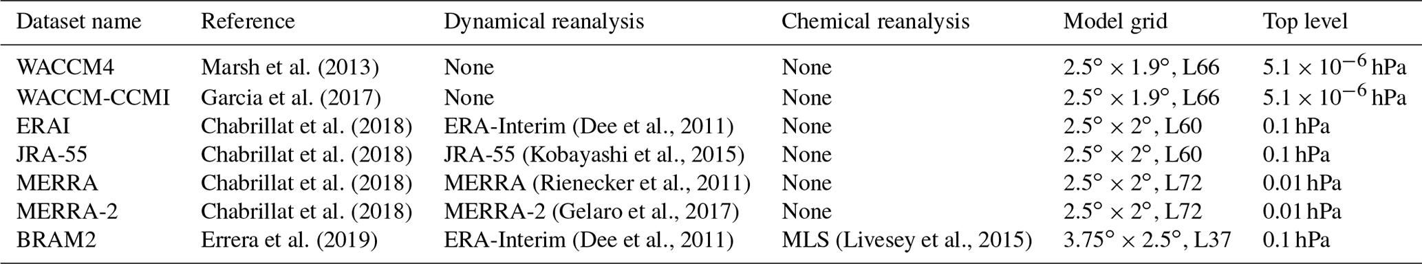
This work uses seven datasets that were generated by WACCM, the BASCOE CTM and the BASCOE DAS. Table 1 provides an overview of these datasets and their main differences, and the next three subsections provide details about the models and systems that generated them.
2.1 WACCM
WACCM (Garcia et al., 2017) is the atmospheric component of the Community Earth System Model version 1.2.2 (Hurrell et al., 2013), which has been developed by the U.S. National Center for Atmospheric Research. It is the extended (whole atmosphere) version of the Community Atmosphere Model version 4 (CAM4; Neale et al., 2013).
We ran one realization of the public version of WACCM (hereafter WACCM4; Marsh et al., 2013) with a similar setup (e.g., lower boundary conditions) to the CTM experiments; the source code of WACCM4 is available for download at https://svn-ccsm-models.cgd.ucar.edu/cesm1/release_tags/cesm1_2_2/, last access: 28 October 2020. In this study we also use three realizations of the REF-C1 simulation used in the SPARC Chemistry-Climate Model Initiative (CCMI; Morgenstern et al., 2017). The CCMI experiments, hereafter WACCM-CCMI, differ from WACCM4 with respect to the modified gravity wave parameterization and the updated heterogenous chemistry (Garcia et al., 2017). The inclusion of WACCM4 allows us to carry out a sensitivity test regarding the impact of the modified gravity wave parameterization on the simulation of the N2O transport (see Sect. 4 for detailed analysis). We use 3-D daily mean output over the 2005–2014 period to allow a fair comparison with the BRAM2 dataset (see Sect. 2.3 for detailed analysis). WACCM has a longitude–latitude grid of and 66 vertical levels ranging from the surface to an altitude of about 140 km. The vertical coordinate is hybrid-pressure, i.e., terrain-following below 100 hPa and purely isobaric above this level. The vertical resolution depends on the height: it is approximately 3.5 km above 65 km, 1.75 km around the stratopause (50 km), 1.1–1.4 km in the lower stratosphere (below 30 km) and 1.1 km in the troposphere. The time step for the physics in the model is 30 min.
The physics of WACCM is the same as CAM4, and the dynamical core is a finite volume with a horizontal discretization based on a conservative flux-form semi-Lagrangian (FFSL) scheme (Lin, 2004). The gravity wave parameterization accounts for momentum and heat deposition separating orographic and non-orographic sources. The orographic waves are modified according to Garcia et al. (2017), whereas non-orographic waves are parameterized depending on the convection and the frontogenesis occurrence in the model (Richter et al., 2010).
In this study, the WACCM versions considered are not able to internally generate the quasi-biennial oscillation (QBO; see, e.g., Baldwin et al., 2001). Thus, the QBO is nudged by a relaxation of stratospheric winds to observations in the tropics (Matthes et al., 2010). The solar forcing uses the Lean et al. (2005) approach.
WACCM includes a detailed coupled chemistry module for the middle atmosphere based on the Model for Ozone and Related Chemical Tracers, version 3 (MOZART-3; Kinnison et al., 2007; Marsh et al., 2013). The species included within this mechanism are contained within the Ox, NOx, HOx, ClOx and BrOx chemical families, along with CH4 and its degradation products. In addition, 20 primary non-methane hydrocarbons and related oxygenated organic compounds are represented along with their surface emission. There are a total of 183 species and 472 chemical reactions; this includes 17 heterogeneous reactions on multiple aerosol types, i.e., sulfate, nitric acid trihydrate and ice. In WACCM-CCMI the heterogeneous chemistry is updated by Solomon et al. (2015).
2.2 BASCOE CTM
The BASCOE data assimilation system (Errera et al., 2019) is built on a chemistry transport model, which consists in a kinematic transport module with the FFSL advection scheme (Lin and Rood, 1996) and an explicit solver for stratospheric chemistry, comprising 65 species and 243 reactions (Prignon et al., 2019). Chabrillat et al. (2018) explain in detail the preprocessing procedure that allows the BASCOE CTM to be driven by arbitrary reanalysis datasets as well as the setup of model transport. As usual for kinematic transport modules, the FFSL scheme only needs the surface pressure and horizontal wind fields from reanalyses as input, because it is set on a coarser grid than the input reanalyses, and relies on mass continuity to derive vertical mass fluxes corresponding to its own grid. Similar to Chabrillat et al. (2018), the model is driven by four different reanalysis datasets on a common, low-resolution, latitude–longitude grid (), but it retains their native vertical grids. In this way, we avoid any vertical regridding, and the intercomparison explicitly accounts for the different vertical resolutions.
The four input reanalyses, the European Centre for Medium-Range Weather Forecasts Interim reanalysis (ERA-Interim, hereafter ERAI; Dee et al., 2011), the Japanese 55-year Reanalysis (JRA-55; Kobayashi et al., 2015), and the Modern-Era Retrospective analysis for Research and Applications (MERRA; Rienecker et al., 2011) and its version 2 (MERRA-2; Gelaro et al., 2017), are part of the SPARC Reanalysis Intercomparison Project (S-RIP), which is a coordinated intercomparison of all major global atmospheric reanalyses, and they are described in Fujiwara et al. (2017). ERAI and JRA-55 have 60 levels up to 0.1 hPa while MERRA and MERRA-2 have 72 levels up to 0.01 hPa. The CTM time step is set to 30 min. As for the WACCM experiment, we used the daily mean outputs from the BASCOE CTM over the 2005–2014 period.
2.3 BASCOE reanalysis
BRAM2 is the BASCOE reanalysis of Aura MLS, version 2, which covers the period from August 2004 to August 2019 (Errera et al., 2019). For BRAM2, BASCOE is driven by dynamical fields from ERA-Interim, with a (longitude × latitude) horizontal resolution. The vertical grid is represented by 37 hybrid-pressure levels which are a subset of the ERA-Interim 60 levels.
In BRAM2, N2O profiles from the MLS version 4 standard product have been assimilated within the 0.46–68 hPa pressure ranges (Livesey et al., 2015). This dataset is retrieved from the MLS 190 GHz radiometer instead of the 640 GHz radiometer in an earlier MLS version. The 640 GHz radiometer, which provided a slightly better quality retrieval down to 100 hPa, ceased to be delivered after August 2013 because of instrumental degradation in the band used for that retrieval. To avoid any artificial discontinuity due to switching from one product to the other in August 2013, BRAM2 has assimilated the 190 GHz N2O during the whole reanalysis period.
BRAM2 N2O has been validated between 3 and 68 hPa against several instruments with a general agreement within 15 % depending on the instrument and the atmospheric region (the middle stratosphere or the polar vortex; see Errera et al., 2019). It is not recommended to use the BRAM2 N2O reanalysis outside of this pressure range. BRAM2 N2O is also affected by a small drift of around −4 % between 2005 and 2015 (see also Froidevaux et al., 2019).
2.4 TEM diagnostics
For atmospheric tracers, the TEM analysis (Andrews et al., 1987) allows for the separation of the local change in a tracer with the volume mixing ratio χ in terms of transport and chemistry (Eq. 1).
where χ is the volume mixing ratio of N2O, and M is the eddy flux vector, which is defined as
and are the meridional and vertical components of the residual mean meridional circulation, respectively, and they are defined as
Here, , and are the Eulerian zonal-mean meridional and vertical velocities and the potential temperature, respectively; ϕ is the latitude; and S is the net rate of change due to chemistry, i.e., , where and are the respective zonal-mean chemical production and loss rates. Overbar quantities represent zonal-mean fields, primed quantities represent the departures from the zonal mean and subscripts denote derivatives. Meridional derivatives are evaluated in spherical coordinates and vertical derivatives with respect to log-pressure altitude , with ps=105 Pa and H=7 km.
Hence, transport is separated into advection due to the residual circulation (first two terms on the right-hand side, RHS, of Eq. 1) and irreversible quasi-horizontal isentropic eddy mixing, .
In order to better understand the role of each term in the tracer balance, it is useful to separate the components of the vector M and rearrange the terms of Eq. (1) as follows:
where
Here, Ay represents the meridional residual advection, My represents the horizontal transport due to eddy mixing, Az represents the vertical residual advection and Mz represents the vertical eddy mixing (all expressed in ppbv d−1). It is important to note that the total mixing term (My+Mz) includes not only the effects of irreversible mixing but also some effects of the advective transport that are not resolved by the residual advection (Andrews et al., 1987; Holton, 2004).
Before any TEM calculation, all of the input fields are interpolated to constant pressure levels from the hybrid-sigma coefficients, which retain the same vertical resolution as the original vertical grid of each dataset (Table 1). Each derivative is computed using a centered differences method.
In addition to the physical TEM terms (Eq. 1), it is necessary to include an additional term on the RHS of Eq. (4): the residual term ϵ. It is the difference between the actual rate of change of χ (LHS of Eq. 4) and the sum of all of the transport and chemical terms of the TEM budget. This nonzero residual has several causes (Abalos et al., 2017). The TEM calculations for WACCM rely on the diagnostic variable w, which is not used to advect the tracers, because the model is based on a finite volume dynamical core (Lin, 2004). Furthermore, an implicit numerical diffusion is added to the transport scheme in WACCM in order to balance the small-scale noise without altering the large-scale features. This numerical diffusion is not included in the TEM budget and is larger in regions with large small-scale features, i.e., regions where gradients are stronger (Conley et al., 2012). All TEM calculations are done using daily mean data, even though WACCM and BASCOE both run with a much smaller time step of 30 min. The daily mean fields are interpolated from their native hybrid-sigma levels to constant pressure levels prior to the TEM analysis, leading to numerical errors in the lower stratosphere. The BASCOE datasets have a coarser horizontal resolution than their input reanalyses (especially BRAM2; see Table 1). This affects the accuracy of the vertical and horizontal derivatives, with possible implications for the residual. The possible causes of the residual in the five reanalysis datasets are discussed in more detail in Sect. 3. For WACCM-CCMI, the TEM budget is computed for each realization, allowing for the examination of both the ensemble mean (e.g., for seasonal means) or the model envelope (e.g., for line plots). In order to validate our N2O TEM budget, we reproduced the findings reported in Tweedy et al. (2017, Fig. 7) with WACCM-CCMI in the tropical lower stratosphere, and we noticed similar results (not shown).
In order to interpret the TEM analysis of the N2O budget, we also compute the Eliassen–Palm flux divergence (EPFD). The Eliassen–Palm flux is a 2-D vector defined as (Andrews et al., 1987), with its meridional and vertical components, respectively, given by
The EPFD reflects the magnitude of the eddy processes and provides a direct measure of the dynamical forcing of the zonal-mean state by the resolved eddies (Edmon et al., 1980).
The four dynamical reanalyses used in this study provide overall consistent temperature and winds in the stratosphere, but they can lead to a different representation of large-scale transport (e.g., Chabrillat et al., 2018) due to the biases in the temperature and wind fields (Kawatani et al., 2016; Tao et al., 2019). Note that the TEM quantities are not directly constrained by observations, especially the upwelling velocity , that can vary considerably in the dynamical reanalyses, as it is a small residual quantity (Abalos et al., 2015).
In the rest of the paper, we will assume that the BRAM2 product provides the best available approximation of the TEM budget for N2O – at least where the residual is smaller than the vertical advection and horizontal mixing terms. This assumption relies on the combination in BRAM2 of dynamical constraints from ERA-Interim and chemical constraints from MLS (Errera et al., 2019).

Figure 1Latitudinal profiles of the N2O TEM budget terms at 15 hPa averaged in DJF (2005–2014) with WACCM-CCMI (a), JRA-55 (b), MERRA-2 (c), MERRA (d), ERAI (e) and BRAM2 (f). The color code is shown in the legend. Units are in parts per billion by volume per day (ppbv d−1).

Figures 1 and 2 show the N2O TEM budget terms at 15 hPa for all of the datasets for the boreal winter (December–January–February, DJF, mean) and summer (June–July–August, JJA, mean), respectively. The 15 hPa level (around 30 km altitude) was chosen because large differences can be found between WACCM-CCMI, BRAM2 and the CTM runs at this level and because the dynamical reanalyses are not constrained as well by meteorological observations at higher levels (Manney et al., 2003). Figures 1 and 2 aim to show how the dynamical and chemical terms of the budget balance each other to recover the tendency at different latitudes. A discussion on the differences between the datasets and their possible physical causes is given in the next sections.
The vertical advection term Az shows how the upwelling contributes to increasing the N2O abundances in the tropics and summertime midlatitudes and how polar downwelling contributes to decreasing the N2O abundances in the winter hemisphere. The horizontal transport out of the tropics due to eddies, as represented by My, reduces the N2O abundance in the tropical latitudes of the wintertime hemisphere and increases the N2O mixing ratio at high latitudes in the winter hemisphere. The other terms of the TEM budget are weaker than Az and My: the meridional advection term Ay tends to increase the N2O abundance in the winter subtropics and extra-tropics; the vertical transport term due to eddy mixing, Mz, decreases the N2O mixing ratio over the northern polar latitudes; and the chemistry term P−L shows that N2O destruction by photodissociation and O(1D) oxidation contributes to the budget in the tropics and also in the summertime hemisphere. All budget terms are weaker in the summer hemisphere than in the winter hemisphere. Over the southern polar winter latitudes, the reanalyses deliver negative My that are balanced by large positive residuals, which implies a less robust TEM balance (Fig. 2). This is not the case with WACCM, where My tends to increase the N2O abundance in the polar vortex. Such differences between the datasets are highlighted and discussed in the next sections.
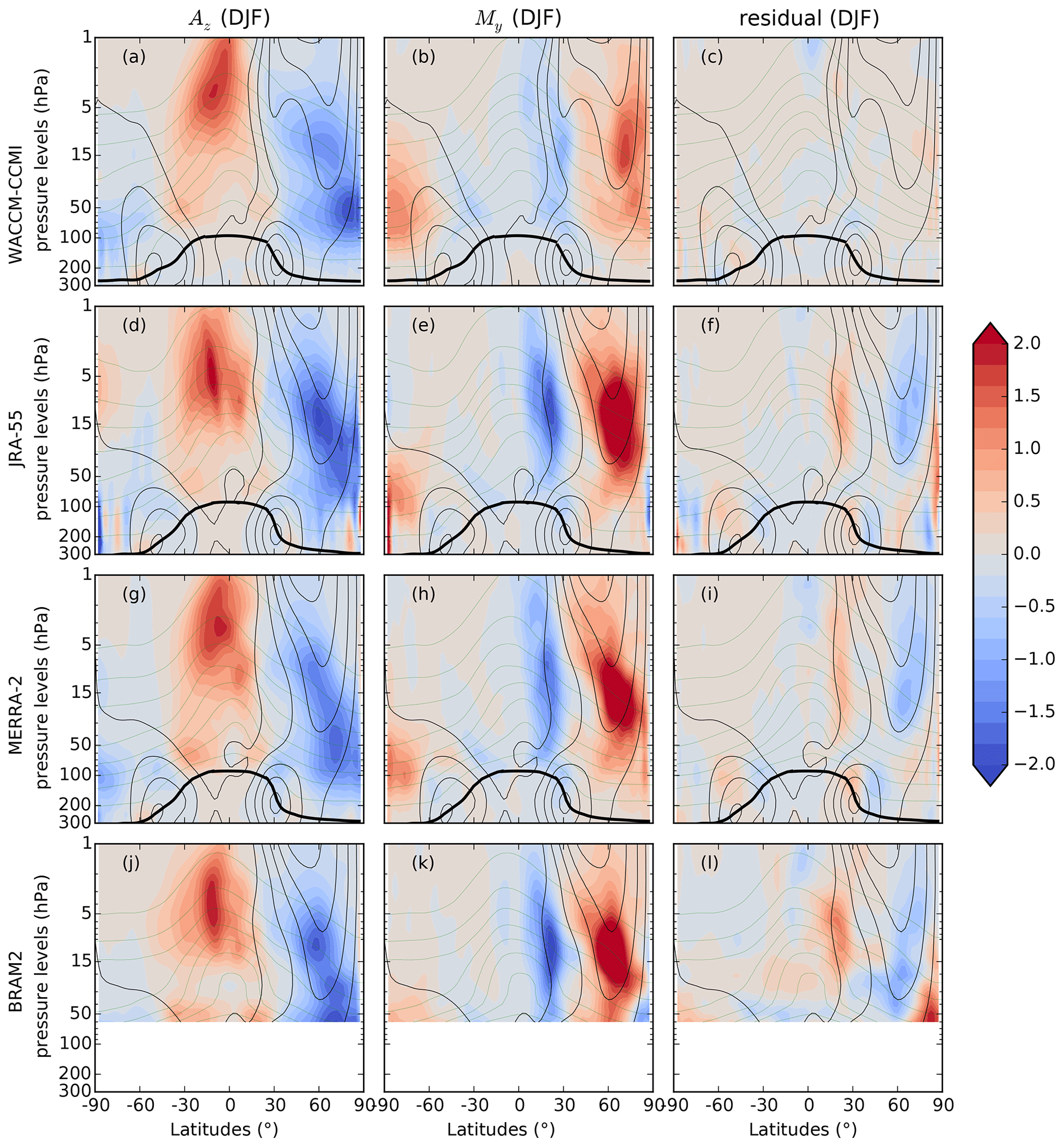
Figure 3Climatological (2005–2014) latitude–pressure cross sections of three N2O TEM budget terms averaged in DJF (ppbv d−1) for the horizontal mixing term (a, d, g, j), the vertical residual advection term (b, e, h, k) and the residual term (c, f, i, l). The datasets are, from top to bottom, WACCM-CCMI, JRA-55, MERRA-2 and BRAM2. The residual term for WACCM-CCMI is from a single realization of the model. The thin black lines show the zonal-mean zonal wind (from 0 to 40 m s−1 every 10 m s−1), the black thick line represents the dynamical tropopause for the considered season and the green thin lines show the climatological mixing ratio of N2O (from 20 to 300 ppbv with 40 ppbv spacing).
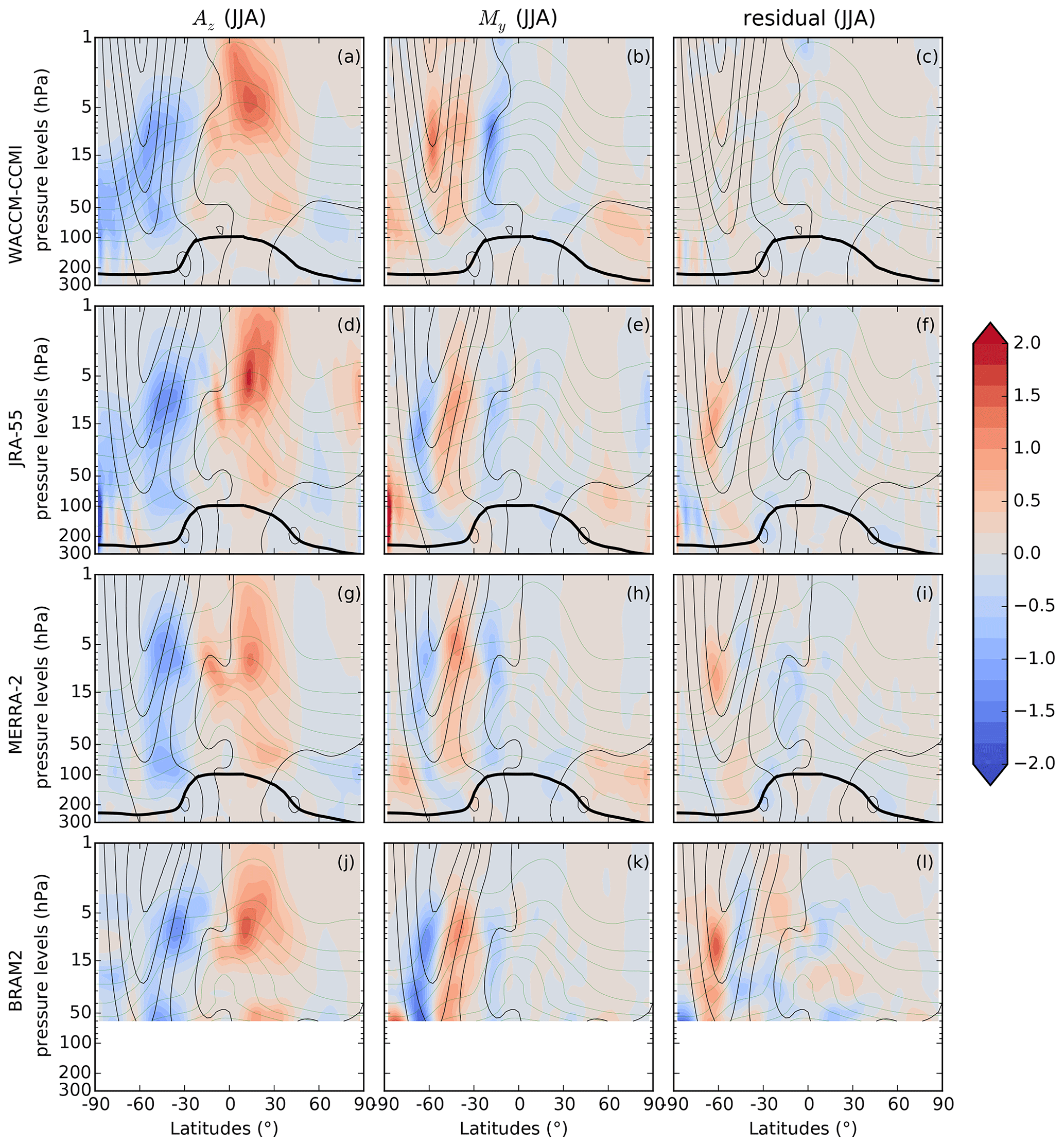
Figure 4Same as Fig. 3 but for JJA and with a different color scale. The thin black contours show the zonal-mean zonal wind (from 0 to 100 m s−1 every 20 m s−1).
Figures 3 and 4 show the DJF and JJA means of three contributions to the N2O TEM budget, respectively, namely the horizontal mixing My, the vertical advection Az and the residual terms ϵ, for WACCM-CCMI, JRA-55, MERRA-2 and BRAM2. For those datasets, the remaining terms of the TEM budget (Ay, Mz and P−L) for DJF and JJA are shown in Supplement Figs. S1 and S2, respectively. The full N2O TEM budgets obtained with MERRA and ERAI for DJF and JJA are shown in Figs. S3 and S4, respectively. In the case of WACCM-CCMI, the seasonal means were computed separately for each realization, and we verified that the ensemble means show the same features as the individual realizations. Large differences arise in the dynamical terms of the TEM budget between summer and winter for both hemispheres in the extra-tropics. The strong seasonality of the deep branch of the BDC and of the transport barriers are the causes of these differences, as for the seasonal variations of the age of air spectrum (Li et al., 2012).
We also reproduced the results of Randel et al. (1994, Fig. 8) for the WACCM-CCMI multi-model mean and the reanalysis mean in DJF (Figs. S5 and S5, respectively). The WACCM-CCMI and the reanalysis means agree with the Community Climate Model version 2 of the early 1990s with regard to the general pattern of the TEM terms, although both deliver stronger contributions, especially the reanalyses mean.
We first compare the contribution of Az across the datasets in Figs. 3 and 4. The tropical upwelling increases the abundance of N2O mostly in the mid–high stratosphere (between 1 and 15 hPa) with the maximum contribution in the summer tropics, whereas the downwelling decreases it mostly in the wintertime extra-tropics in the middle and low stratosphere (between 5 and 100 hPa). This reflects the path followed by the deep branch of the BDC (Birner and Bönisch, 2011). During boreal winter, these features are very similar across all datasets (Fig. 3), but noticeable differences appear during the austral winter (Fig. 4): the tropical upwelling has a larger secondary maximum in the southern tropics with JRA-55 and MERRA-2 than with the other datasets, and the extra-tropical downwelling extends to the South Pole in WACCM-CCMI and JRA-55 whereas it is mostly confined to the midlatitudinal surf zone in the other reanalyses. In the lower stratosphere, Az shows the contribution of the residual advection by the shallow branch of the BDC to the N2O abundances in the winter and summer hemispheres. The two-cell structure, consisting of upwelling of N2O in the subtropics and downwelling in the extra-tropics, consistently agrees across all datasets. The meridional residual advection term Ay contributes to the poleward transport of air masses in the middle stratosphere, mostly during the winter, and its contribution to the N2O TEM budget is weaker than Az. Ay agrees well among the datasets in boreal winter (Figs. S1, S3), while during austral winter WACCM-CCMI overestimates it by around 30∘ S compared with the reanalyses (Figs. S2, S4).
We move now to the mixing contributions to the N2O budget. The horizontal mixing is the predominant contribution to the poleward tracer transport in the middle and lower stratosphere (Abalos et al., 2013), as it flattens the tracer gradients generated by the residual advection. In the N2O TEM budget during boreal winter, My mostly balances the extra-tropical downwelling and part of the tropical upwelling (Figs. S3, S4). The surf zone is characterized by strong horizontal mixing, depicted here as large positive My contributions, and delimited by transport barriers which appear as intense gradients of My in the winter hemispheres (panels b, e, h and k in Figs. 3 and 4). In the wintertime NH, the patterns of My are similar in all datasets (Fig. 3), but the effect of horizontal eddy mixing on N2O is stronger in the reanalyses than in WACCM-CCMI. In Sect. 4, we quantitatively analyze the differences in the mid-stratospheric My between datasets. The residual terms in the reanalyses (Fig. 3c, f, i, l) are largest in the middle stratosphere at the latitudes of the transport barriers, and their signs are opposite to My.
In the austral winter, over the Antarctic polar cap and below 30 hPa, My agrees remarkably well in all datasets (Fig. 4). Closer to the vortex edge and above 30 hPa, the wintertime decrease in N2O is mainly due to downwelling in WACCM-CCMI, whereas the reanalyses, especially BRAM2, show that the horizontal mixing plays a major role (Fig. 4). The impact of horizontal mixing on N2O inside the wintertime polar vortex is not negligible (e.g., de la Cámara et al., 2013; Abalos et al., 2016a), as Rossby wave breaking occurs there as well as in the surf zone. In contrast to the reanalyses, in WACCM-CCMI the My contribution is close to zero in the Antarctic vortex and maximum along the vortex edge (Fig. 4). This disagreement can be related to differences in the zonal wind: it is overestimated in WACCM above 30 km at subpolar latitudes compared with MERRA (Garcia et al., 2017), and the polar jet is not tilted equatorward as in the reanalyses (see black thin lines in Figs. 4 and 3 of Roscoe et al., 2012). However, the differences in My and Az above the Antarctic in winter should be put into perspective with the relatively large residual terms that point to incomplete TEM budgets in the reanalyses (Figs. 4 and S4 right columns). Near the Antarctic polar vortex, the assumptions of the TEM analysis (such as small amplitude waves) are less valid, leading to larger errors in the evaluation of the mean transport and eddy fluxes (Miyazaki and Iwasaki, 2005).
As the relative importance of the residual is considerable above the Antarctic in the reanalyses (Fig. 4), it is necessary to better understand its physical meaning. Dietmüller et al. (2017) applied the TEM continuity equation to the age of air in CCM simulations. Computing the “resolved aging by mixing” (i.e., the AoA counterpart of My+Mz) as the time integral of the local mixing tendency along the residual circulation trajectories and the “total aging by mixing” as the difference between the mean AoA (mAoA) and the residual circulation transit time, they defined the “aging by mixing on unresolved scales” (i.e., by diffusion) as the difference between the latter and the former. This “aging by diffusion”, which can be related by construction to our residual term, arises around 60∘ S from the gradients due to the polar vortex edge. Even though we use a real tracer (N2O), we find a qualitative agreement with this analysis based on AoA: our residual term is larger in regions characterized by strong gradients such as the Antarctic vortex edge and larger with dynamics constrained to a reanalysis than with a free-running CCM (see EMAC results in Fig. 1d by Dietmüller et al., 2017). Thus, we interpret the residual as the sum of mixing at unresolved scales and numerical errors (Abalos et al., 2017).
In the summertime lower stratosphere, we note a stronger contribution of My to the N2O abundances above the subtropical jets in both hemispheres and for all datasets compared with higher levels in summer (panels b, e, h and k in Figs. 3 and 4). This behavior is consistent with calculations of the effective diffusivity and age spectra (Haynes and Shuckburgh, 2000; Ploeger and Birner, 2016). It is due to transient Rossby waves that cannot travel further up into the stratosphere owing to the presence of critical lines, i.e., where the phase velocity of the wave matches the background wind velocity, generally leading to wave breaking (Abalos et al., 2016b). In particular, above the northern tropics during the boreal summer (Figs. 4, S2, S4), horizontal mixing is primarily associated with the Asian monsoon anticyclone, and it causes a decrease in N2O (Konopka et al., 2010; Tweedy et al., 2017). In the lower stratosphere, the contributions from My combine with that from Az in the total impact of the shallow branch of the BDC on N2O all year round (Diallo et al., 2012).
The vertical mixing contribution Mz is very small during boreal winter, except in the middle and lower stratosphere poleward of 60∘ N, where it tends to balance the My contribution (Figs. S1, S3). In austral winter, there is a strong disagreement between WACCM-CCMI and the reanalyses around 60∘ S between 5 and 15 hPa (Fig. S2). WACCM-CCMI simulates a strong Mz contribution at the polar jet core that decreases the N2O abundances and tends to balance My, whereas Mz is weaker and increases N2O in the higher stratosphere in the reanalyses.
In the next section, we focus on a single level in the middle stratosphere to quantitatively study the disagreement between WACCM-CCMI and the reanalyses.
After investigating the seasonal means of Az and My, it is interesting to examine their climatological mean annual cycles in order to study the month-to-month variations over the year and their dependance on the latitude in the middle stratosphere. The cycles are shown for three latitude bands in each hemisphere corresponding to the tropics (0–20∘), the surf zones (40–60∘) and the polar regions (60–80∘). For WACCM-CCMI, we examine the envelope (the yellow shaded areas in Figs. 5–12) of the three model realizations in order to evaluate the role of the internal variability and its relative importance for each month and latitude band. In the following, we will consider BRAM2 as the reference when comparing N2O mixing ratios between datasets, because its dynamics and chemistry are both constrained by observational datasets.
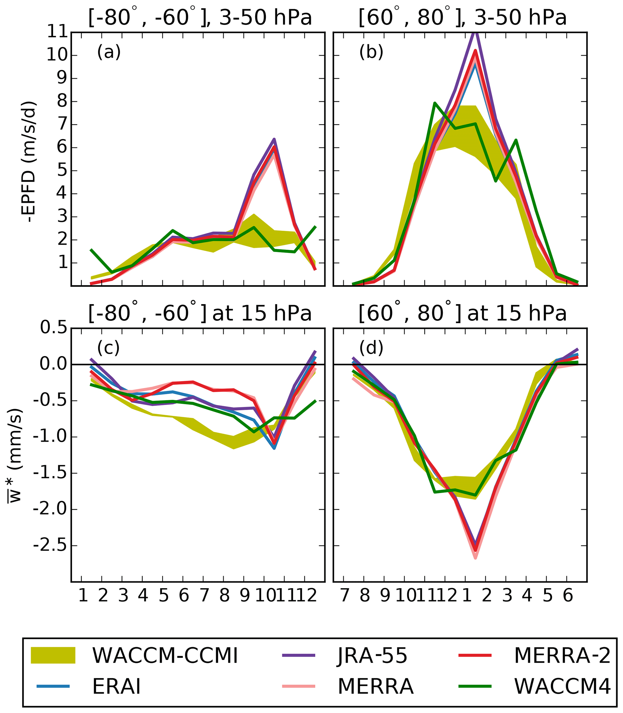
Figure 5Monthly mean annual cycle of (a, b) the EPFD () averaged between 3 and 50 hPa and (c, d) (mm s−1) at 15 hPa for (a, c) the Antarctic region (60–80∘ S) and (b, d) the Arctic region (60–80∘ N). The color code is shown in the legend. The yellow envelope shows the three realizations of the WACCM-CCMI simulation.
4.1 Polar regions
The EPFD is often used to quantify the forcing of the wave drag due to resolved (planetary) waves (e.g., Gerber, 2012; Konopka et al., 2015). We first show the monthly mean climatological annual cycles of EPFD averaged between 3 and 50 hPa and the residual vertical velocity at 15 hPa for the polar regions (60–80∘ S and N, Fig. 5). We arbitrarily average the EPFD between 3 and 50 hPa in order to identify the wave forcing for the deep branch of the BDC (Plumb, 2002; Konopka et al., 2015). However, the qualitative results do not depend on the choice of the lower boundary level. We also show one realization of the earlier version WACCM4 that suffered from a larger cold bias above the Antarctic (see Sect. 2.1). In WACCM-CCMI, the parameterization of gravity waves was adjusted in order to reduce this issue while not significantly changing the dynamics in the NH, which results in an enhanced polar downwelling above the southern polar region (Garcia et al., 2017). Above the Antarctic, the forcing from resolved waves peaks in October in the reanalyses as a result of the vortex breakup that allows enhanced wave activity compared with austral winter (Randel and Newman, 1998). The WACCM simulations miss this strong springtime peak, and they are in good agreement with the reanalyses during the rest of the year (Fig. 5a). The residual vertical velocity w∗ above the Antarctic is shown in Fig. 5c. This comparison between the WACCM versions was already shown in Garcia et al. (2017, Fig. 10), but we repeat it here adding the dynamical reanalyses. In November–December the weaker downwelling in WACCM-CCMI agrees well with the reanalyses. Throughout the rest of the year WACCM-CCMI simulates a stronger downwelling than all reanalyses (also at lower levels, not shown). This difference raises the question of whether the residual vertical velocity is correctly represented in WACCM-CCMI or in the dynamical reanalyses. Above the Arctic, the WACCM simulations underestimate the EPFD contribution during boreal winter compared with the reanalyses (Fig. 5b), and the downwelling velocities simulated by WACCM are weaker than the reanalyses during that period, with no significant differences between the WACCM versions (Fig. 5d). The differences between WACCM and the reanalyses in EPFD and w∗ in the polar regions will help with the interpretation of the differences in Az and My.
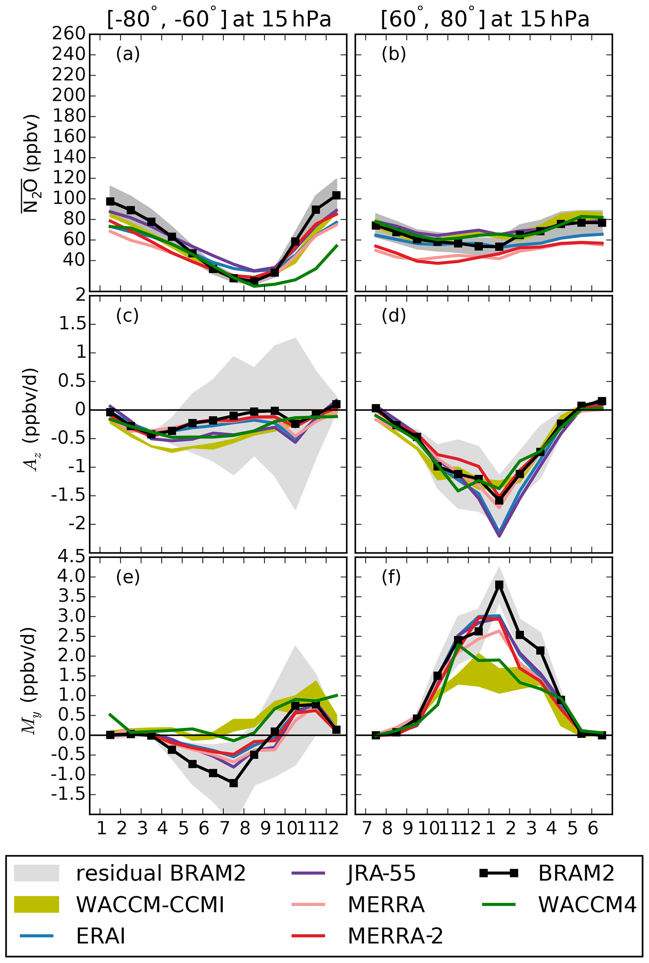
Figure 6Annual cycles over the 2005–2014 period at 15 hPa for (a, b) the N2O volume mixing ratio (ppbv), (c, d) My (ppbv d−1) and (e, f) Az (ppbv d−1) in the (a, c, e) Antarctic region (60–80∘ S) and the (b, d, f) Arctic region (60–80∘ N). Note that the vertical scale differs for My and Az. The olive envelope shows the three realizations of the WACCM-CCMI simulation. The color codes for the four CTM simulations follow the conventions of S-RIP (Fujiwara et al., 2017). BRAM2 is depicted using a black line and symbols, as usually done for observations, because it is constrained by both dynamical and chemical observations. As the N2O mixing ratio in BRAM2 has been evaluated with a 15 % uncertainty (1σ standard deviation) at 15 hPa (Errera et al., 2019), this is highlighted by a dark gray region in panels (a) and (b). The light gray shading around the BRAM2 cycles represents the uncertainty arising from the residual term in the TEM budget, i.e., it is entirely interpreted first as an uncertainty on Az and then as an uncertainty on My in order to remain cautious.
Figure 6 shows the monthly mean climatological annual cycle of the N2O mixing ratio, Az and My for the polar regions (60–80∘ S and N) at 15 hPa for all of the datasets. First, we investigate the N2O mixing ratio in the Antarctic region (Fig. 6a). During winter, the N2O abundances are smaller than the rest of the year due to the suppressed transport from the lower latitudes caused by the onset of the polar barrier. After the vortex breakup, the N2O increase during spring and early summer is smaller in all of the simulations than in BRAM2. In WACCM-CCMI, the modification of the parameterization of gravity waves also results in a shift towards earlier vortex breakup dates in the austral spring compared with WACCM4 (Garcia et al., 2017). The earlier vortex breakup in WACCM-CCMI allows for the transport of N2O-rich air from lower latitudes for a longer period compared with WACCM4, resulting in larger and more realistic simulations of the N2O mixing ratios during austral spring and early summer (Fig. 6a).
In the Antarctic region, the downwelling decreases N2O during most of the year (Az term in Fig. 6c). Here, JRA-55 and WACCM-CCMI are outliers: both present stronger Az contributions in fall and winter, especially WACCM-CCMI, which reaches values that are 3 times stronger than BRAM2 in early winter, as a result of the stronger downwelling velocity simulated by WACCM-CCMI in that region. While this strong disagreement is questioned by the large residuals, we note that all of the reanalyses confirm it except JRA-55. During fall and summer, Az is stronger in WACCM-CCMI than in WACCM4 as a consequence of the stronger downwelling in WACCM-CCMI that results from the modification of the gravity wave parameterization.
We now turn to the contribution from My. In the Antarctic region, My is very different among the datasets during winter: in BRAM2 it contributes to the N2O decrease during fall and winter, with the strongest contribution in July; however, this contribution is 2 times weaker with the CTM simulations, and the horizontal mixing has almost no effect on N2O in WACCM-CCMI (Fig. 6e). As already mentioned, the TEM analysis suffers from large residuals in the wintertime Antarctic region. Nevertheless, we note that the disagreement between WACCM-CCMI and BRAM2 is significant, because the envelope of WACCM-CCMI realizations falls completely outside of the possible BRAM2 values in fall and winter when accounting for the residual. During the austral spring, the vortex breakup leads to an increased wave activity reaching the Antarctic, and My is in better agreement among all datasets compared with austral winter. Note that WACCM-CCMI exhibits large internal variability in this season (Fig. 6e).
It is interesting to highlight the differences between the wintertime Arctic and Antarctic regions, because the hemispheric differences in wave activity (Scaife and James, 2000; Kidston et al., 2015) play a crucial role in the N2O abundances and TEM budget. Above the Arctic, the N2O abundances simulated by WACCM agree with the BRAM2 reanalysis, except in December and January, and the CTM experiments driven by MERRA and MERRA-2 deliver smaller N2O mixing ratios compared with BRAM2 (Fig. 6b). Az is also in good agreement between the datasets above the Arctic, with the exception of ERAI and JRA-55 which provide stronger contributions (Fig. 6d). The Arctic is characterized by a very variable polar vortex with a shorter life span than the Antarctic vortex (Randel and Newman, 1998; Waugh and Randel, 1999), resulting in an enhanced contribution of the horizontal mixing to the N2O budget during winter compared with the Antarctic (Fig. 6f). In contrast to the dynamical reanalyses and BRAM2, WACCM shows a 2-fold underestimation of the N2O changes in the Arctic due to horizontal mixing during winter. Note that the Arctic extended winter presents the largest internal variability compared with the other regions, as shown by the spread in the WACCM realizations. The weaker contribution from My in WACCM is meaningful because the relative importance of the residual term is small in the NH. The horizontal mixing is predominately influenced by the forcing from the breaking of resolved (planetary) waves (Plumb, 2002; Dietmüller et al., 2018). In the Arctic region, WACCM underestimates the forcing from resolved waves compared with the dynamical reanalyses in the middle stratosphere (see Fig. 5d). This discrepancy in the resolved wave driving could contribute to the large differences in the wintertime My between the CCM simulations and the CTM experiments above the Arctic. On the other hand, the role of different waves in driving mixing processes is an ongoing research topic, and additional data and sensitivity tests are needed in order to establish a clear separation of the waves' contributions (e.g., gravity wave parameterization, spatial resolution, etc.; Dietmüller et al., 2018). It should also be emphasized that WACCM is among the CCMI models with the lowest contribution of aging by mixing to the age of air (Fig. 2 in Dietmüller et al., 2018).
4.2 Middle latitudes
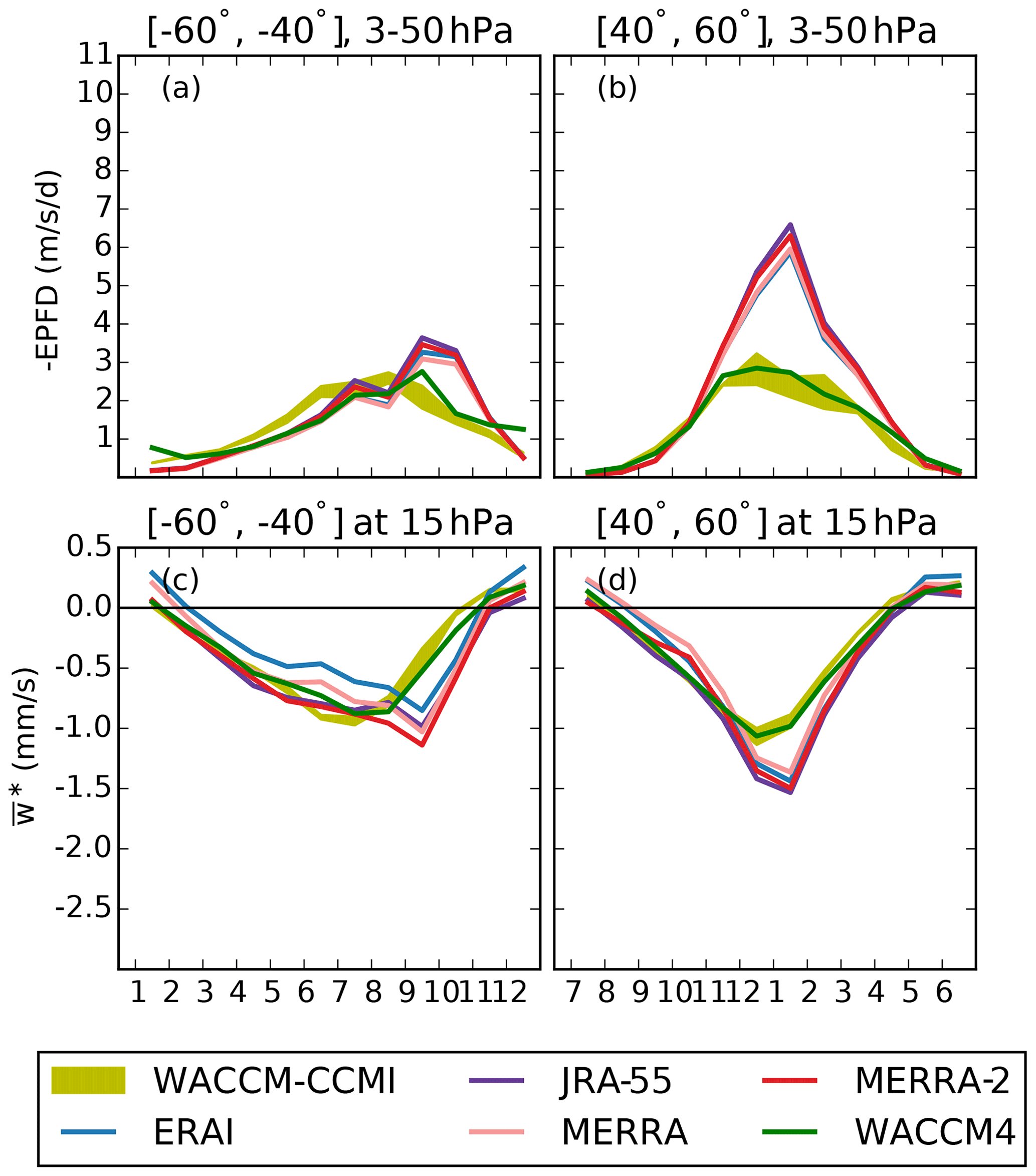
Figure 7 shows the monthly mean climatological annual cycle of w∗ at 15 hPa and the EPFD averaged between 3 and 50 hPa over the surf zones (40–60∘ S and N), and Fig. 8 shows the monthly mean climatological annual cycle of the N2O mixing ratio, Az and My at 15 hPa averaged over the same latitudes. The subtropical barriers are not shown because My and Az change sign in these regions and averaging across the regions would hinder the interpretation of their means.
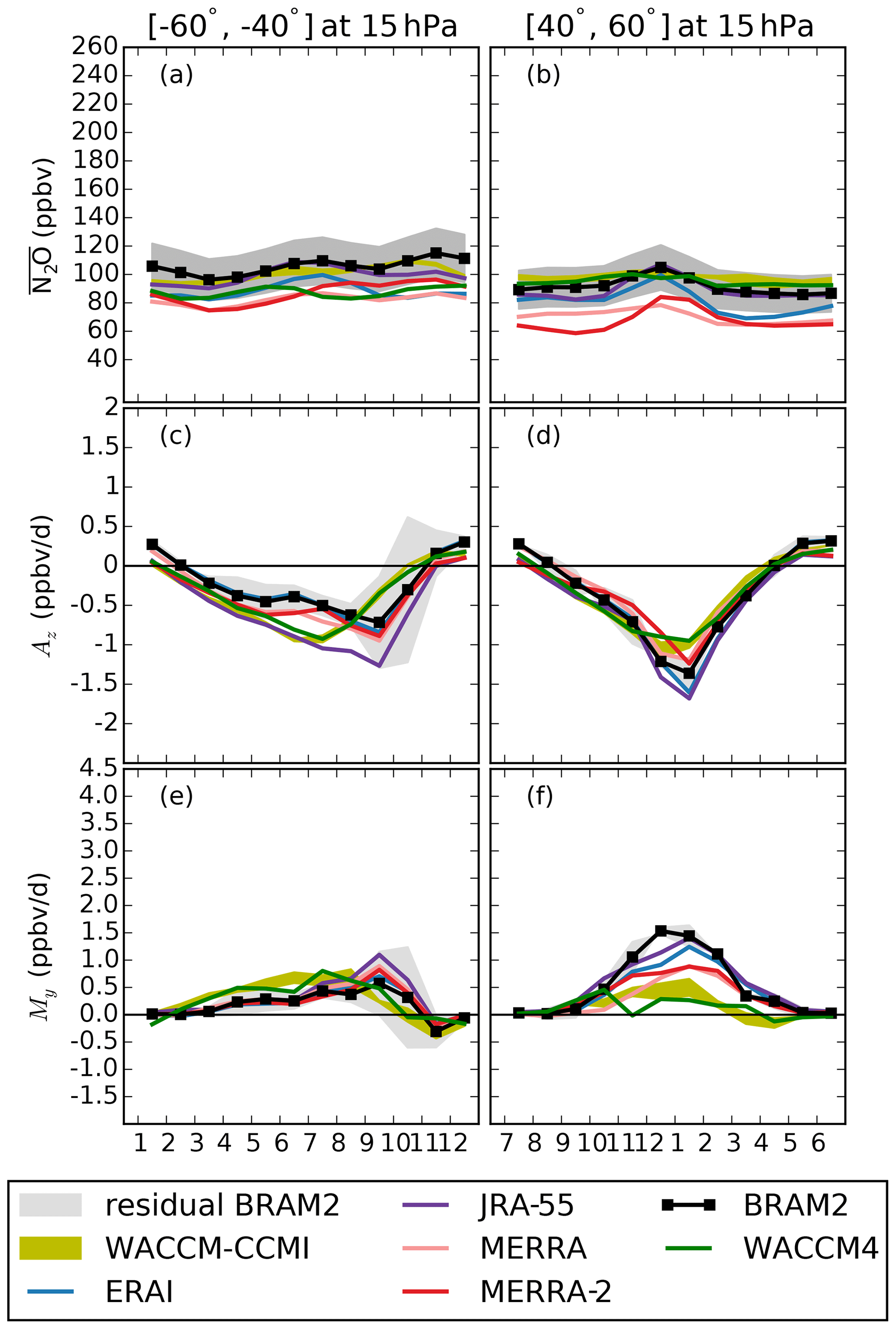
Figure 8As for Fig. 6 but for the middle latitudes: (a, c, e) southern midlatitudes (40–60∘ S); (b, d, f) northern midlatitudes (40–60∘ N).
In the southern midlatitudes, the EPFD peaks in austral spring in the reanalyses, due to the enhanced wave activity in the Southern Hemisphere (SH) during austral spring compared with winter (Konopka et al., 2015), whereas the WACCM simulations deliver an earlier and weaker peak during austral winter (Fig. 7a). The downwelling velocity w∗ shows a similar pattern to the EPFD (Fig. 7c), as it is also driven by the breaking of resolved waves (Abalos et al., 2015). In the northern midlatitudes, the EPFD peaks in winter in all of the datasets, reflecting the stronger wave forcing in the surf zone in this season, and WACCM simulates lower EPFD values compared with the reanalyses (Fig. 7b) that leads to a weaker downwelling velocity in the WACCM simulations (Fig. 7d). As for the polar regions, the differences in EPFD and w∗ between the WACCM simulations and the reanalyses will help with the interpretation of the differences in Az and My.
With regard to the N2O mixing ratio in both hemispheres, the CTMs driven by JRA-55 and ERAI are in good agreement with BRAM2, whereas MERRA-2 and MERRA underestimate it (Fig. 8a, b). The WACCM-CCMI simulations agree well with the BRAM2 chemical reanalysis, confirming the results obtained through the direct comparison with MLS observations (Froidevaux et al., 2019).
We now investigate the contribution from Az and My. In the southern midlatitudes, Az is negative in all seasons except during summer and there is again a good agreement among the datasets except for WACCM-CCMI and JRA-55 (Fig. 8c). These two datasets appear to have a purely annual cycle in this region, whereas the other four show a semiannual component. The peak in the Az contribution in the reanalyses in September results from the increased forcing from the resolved waves (see Fig. 7a) and from the stronger contribution from gravity waves to the mass flux during spring (Sato and Hirano, 2019, Fig. 11). In the same region, My increases throughout the winter, reflecting the mixing associated with the surf zone, and also peaks in early spring in the reanalyses (Fig. 8e). During summer and early fall, My does not contribute significantly to the TEM budget, and My reaches negative values in November which are comparable to the residual term. Both Az and My peak in mid-winter in the WACCM-CCMI simulations, whereas these maxima are reached 3 months later in the reanalyses. This difference is related to the earlier minimum in the downwelling velocity simulated by WACCM-CCMI (see Fig. 7c), which directly affects Az (Fig. 8c) and, due to compensation, My (Fig. 8e). Among the reanalyses, the compensating contributions of Az and My are stronger for JRA-55 than for the other reanalyses (up to 2 times larger in September, see Fig. 8c, e). This reflects the strong BDC in JRA-55 that resulted in the youngest mean AoA in the whole stratosphere (Chabrillat et al., 2018).
In the northern middle latitudes, Az shows the effect of the wintertime downwelling to lower levels on N2O, with the WACCM experiments simulating a slightly weaker contribution than the reanalyses (Fig. 8d). Such disagreement mostly originates from the weaker downwelling velocity in the CCM compared with the reanalyses shown in Fig. 7b. In the northern midlatitudes, the strong My contribution tends to increase the N2O abundances in the surf zone during winter (Fig. 8f). The reanalyses show a large spread, with values reaching ∼1.5 in BRAM2 and ∼0.9 ppbv d−1 in the MERRA runs, and WACCM-CCMI presents a large underestimation with respect to the reanalyses. While the spread across the reanalyses cannot be explained by the forcing from the resolved waves, the weaker My contribution simulated by WACCM could be partly attributed to the weaker EPFD in the CCM compared with the reanalyses (see Fig. 7d).
4.3 Tropics
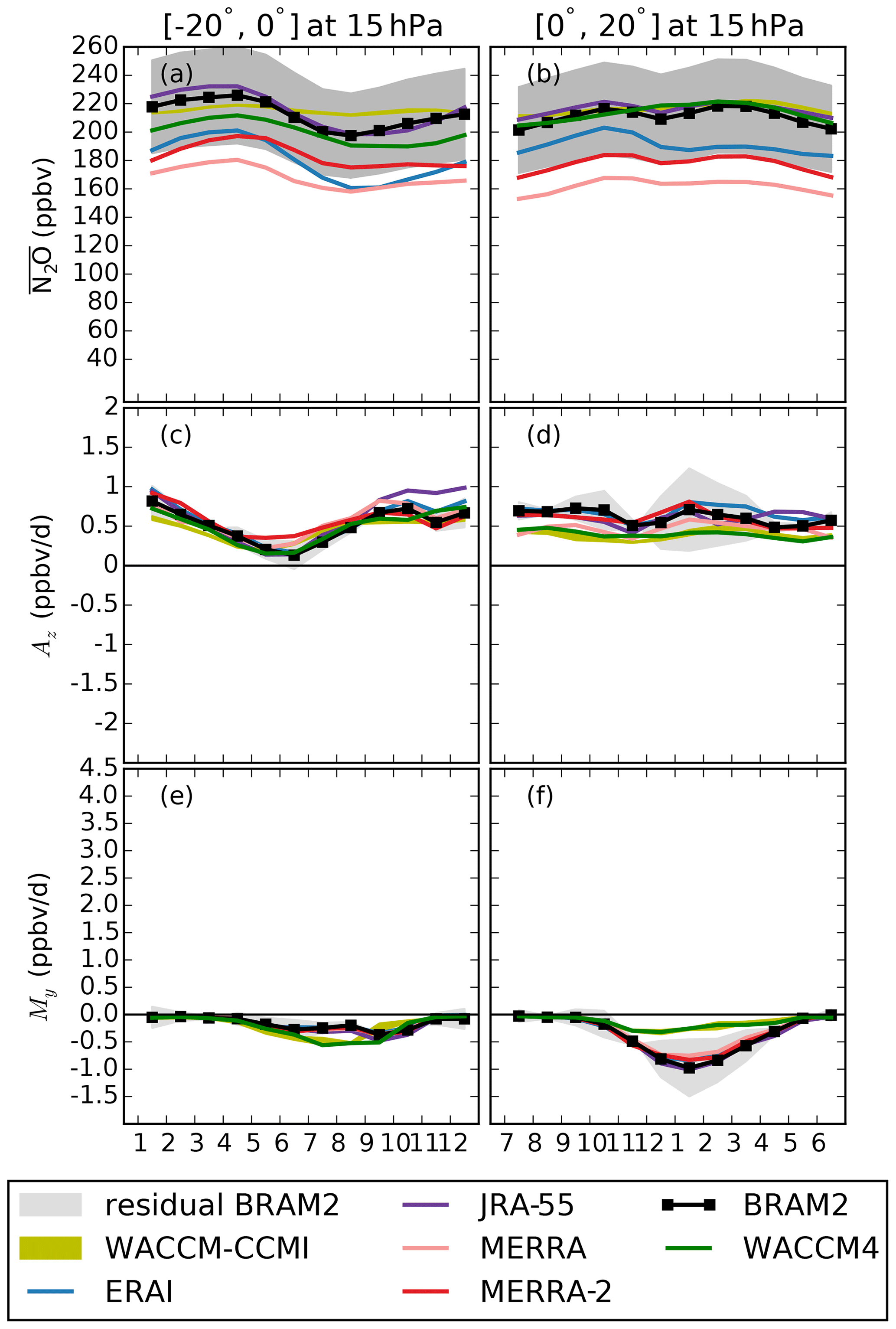
Figure 9 shows the climatological annual cycle for the N2O mixing ratio, Az and My for the southern and northern tropics (0–20∘ S and N) at 15 hPa across all of the datasets. The same latitude bands for the cycles of w∗ and EPFD are shown in the Supplement (Fig. S7). In the tropical regions, the N2O mixing ratio in WACCM-CCMI agrees well with the reanalysis of the Aura MLS, whereas the CTM results show large differences in the N2O abundances depending on the input reanalysis (Fig. 9a, b). In regions where the AoA is less than 4.5 years and N2O is greater than 150 ppb, i.e., in the tropical regions and lower stratospheric middle latitudes (Strahan et al., 2011), the N2O mixing ratio is inversely proportional to the mAoA, because faster upwelling (younger air) implies more N2O transported from lower levels, decreasing its residence time and resulting in a limited chemical destruction (Hall et al., 1999; Galytska et al., 2019). The dynamical reanalyses also produce large differences in mAoA at 15 hPa: MERRA delivers the oldest mAoA, and MERRA-2, ERAI and JRA-55 progressively show a younger mAoA (Fig. 4b in Chabrillat et al., 2018). Hence, the large discrepancies in the N2O mixing ratio can be explained by the large differences in the mAoA, while My and Az contribute to rates of change of N2O.
We continue by investigating the contribution from Az. In both of the tropical regions, the upwelling term Az is positive all year round, showing the effect of tropical upwelling, and agrees very well in the reanalyses (Fig. 9c, d), as a result of the good agreement in the tropical upwelling velocity at 15 hPa (Fig. S7 bottom row), and also as depicted by mAoA diagnostics (Fig. 4d in Chabrillat et al., 2018). Large interhemispheric differences arise in the seasonality of Az between the tropical regions. The largest values of Az in the southern tropics are in the boreal late-fall and winter (Fig. 9c), whereas no large seasonal variations can be detected in the annual cycle of the Az in the northern tropics (Fig. 9d). This is the result of the more pronounced seasonality of the upwelling velocity in the southern tropics compared with the northern tropics (Fig. S7 bottom row).
We now turn to the contribution from My. In the southern tropics, My causes a decrease in the N2O abundances from May to October (when N2O is transported to the middle latitudes), and it has a near-zero contribution over the rest of the year, which is generally common in all of the datasets considered (Fig. 9e). The BRAM2 uncertainty is smaller than for the polar region and middle latitudes, indicating better performance of the TEM analysis outside of the high latitudes. In the northern tropics, My is negative from November to April and presents a marked seasonality in the reanalyses that is much weaker in WACCM-CCMI (Fig. 9f). With respect to interhemispheric differences, WACCM disagrees with the reanalyses: according to WACCM, My has a larger impact in the southern tropics than in the northern tropics, but My has a much larger impact in the northern tropics according to the reanalyses (Fig. 9e, f). These interhemispheric differences in the My contributions can be partly attributed to different forcings from the resolved waves between northern and southern tropics. The EPFD presents a stronger seasonality in the northern tropics than in the southern tropics in all of the datasets (Fig. S7 top row), which could partly explain the differences in the seasonality of My in the reanalyses, but it does not impact the My simulated by WACCM.
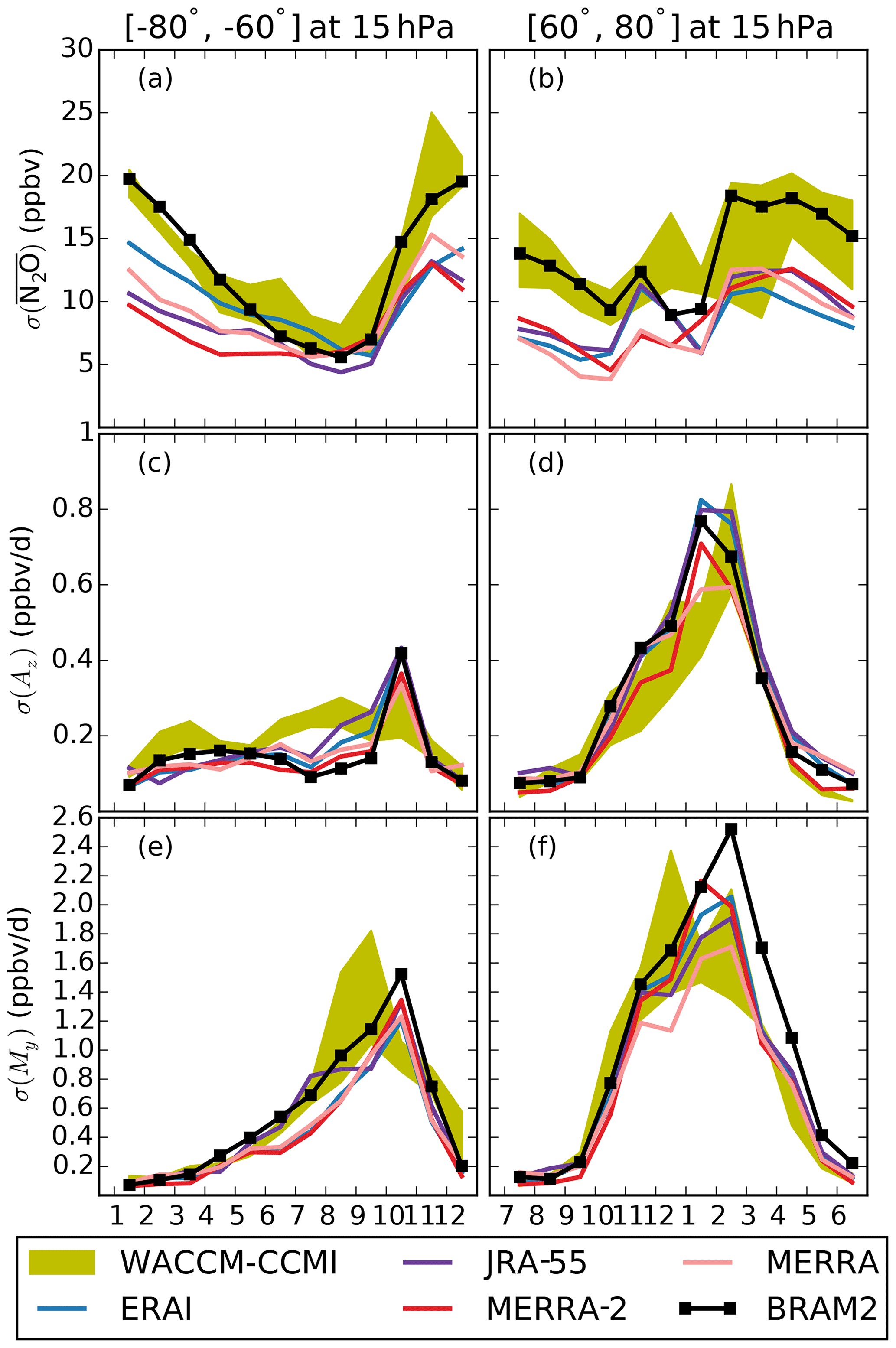
Figure 10Monthly standard deviation over the 2005–2014 period at 15 hPa for (a, b) the N2O volume mixing ratio (ppb), (c, d) the horizontal mixing term (ppbv d−1) and (e, f) the vertical residual advection term (ppbv d−1) in (a, c, e) the Antarctic region (60–80∘ S) and (b, d, f) the Arctic region (60–80∘ N). The color code is shown in the legend. The yellow envelope shows the three realizations of the WACCM-CCMI simulation.
To analyze the interannual variability of the annual cycle, we compute for each month the 1σ standard deviations of the N2O mixing ratio, My and Az across the 10 simulated years. Figure 10 shows the annual cycles of these standard deviations for each dataset in the polar regions (60–80∘ S and N) at 15 hPa for both hemispheres. First, we consider the variabilities of the N2O mixing ratio. In the Antarctic, during austral winter and early spring the year-to-year change in the N2O abundances is very small (Fig. 10a) because the duration, extension and strength of the polar vortex are very stable in a climatological sense, isolating air masses in the vortex from the highly variable midlatitudes (Waugh and Randel, 1999). The variability of the N2O mixing ratio increases in October, i.e., during the breaking vortex period that is highly variable in time (Strahan et al., 2015). Furthermore, the midlatitude air masses, which have more variable composition, become free to reach the higher latitudes during this period. In the Arctic region, the interannual variability of the N2O mixing ratio is also largest during springtime but this is spread over a longer period, i.e., from February to June (Fig. 10b), reflecting the large interannual variability in the duration, extension and zonal asymmetry of the Arctic polar vortex (Waugh and Randel, 1999). In both polar regions, WACCM-CCMI agrees well with BRAM2, whereas the CTM experiments simulate a smaller variability.
We now look at the interannual variability of Az and My in the polar regions. Above the Antarctic, the interannual variabilities of Az and My are maximum during spring (Fig. 10c, e), due to the large interannual variability in vortex breakup dates (Strahan et al., 2015). While the maximum variability of My is consistently reached in October in all of the reanalyses, WACCM-CCMI simulates an earlier maximum (September) that does not correspond to the maximum in its mean values. The lower wintertime variability of both Az and My would increase if a longer period was considered that included the exceptional Antarctic vortices of 2002 (Newman and Nash, 2005) and 2019 (Yamazaki et al., 2019). Above the Arctic, My and Az are most variable during winter, reflecting the frequent disruptions of the northern polar vortex by sudden stratospheric warmings (SSWs; Butler et al., 2017). A case study of the effect of a SSW on the N2O TEM budget showed that Az and My contribute more to this budget during the SSW event than in the seasonal mean (Randel et al., 1994). Thus, the large wintertime variabilities of Az and My are explained by the occurrence of seven major SSWs detected in the reanalyses for the 2005–2014 period (Butler et al., 2017).
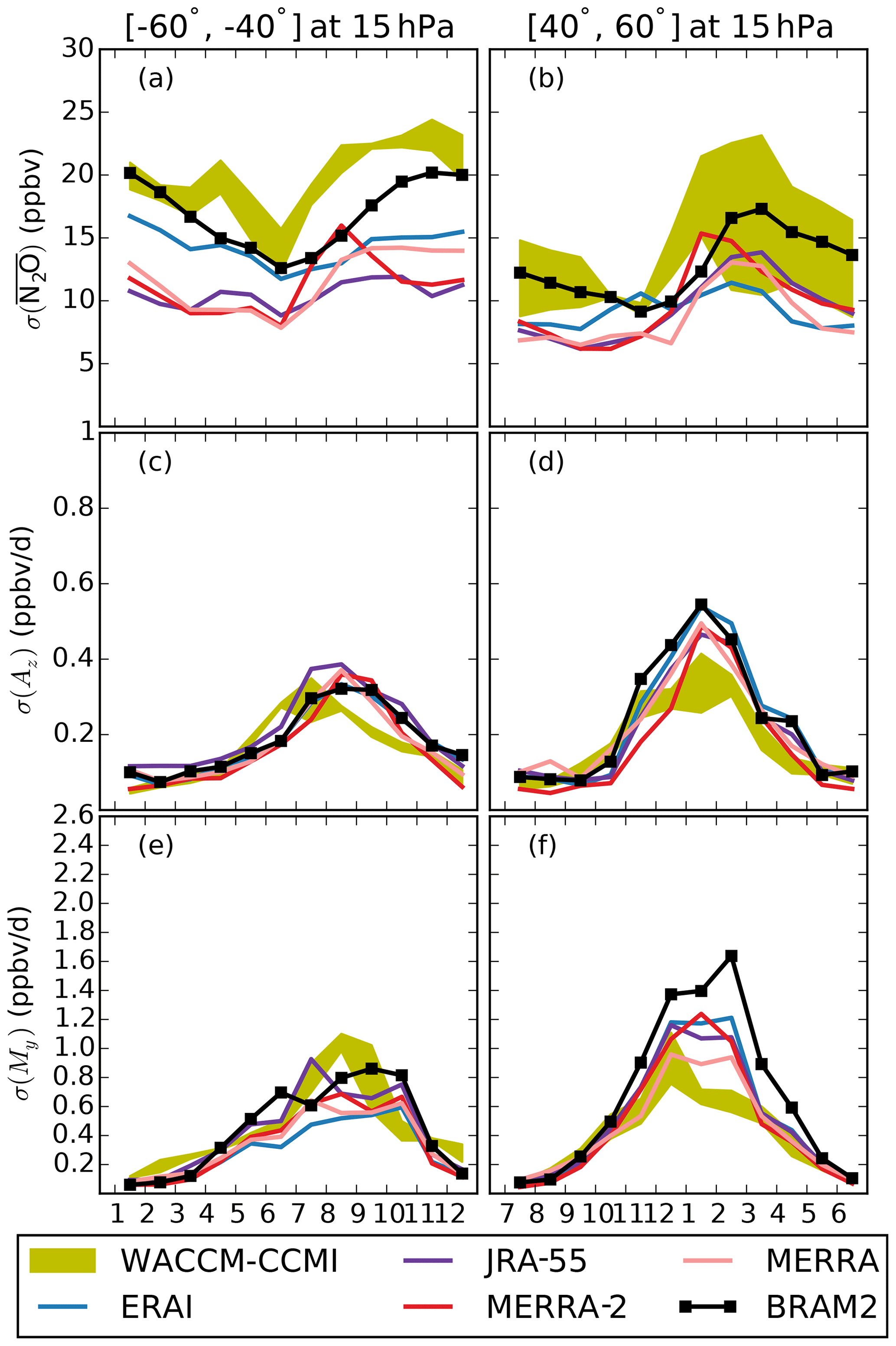
Figure 11As for Fig. 10 but for the middle latitudes: (a, c, e) southern midlatitudes (40–60∘ S); (b, d, f) northern midlatitudes (40–60∘ N).
In Fig. 11, we show the interannual variabilities of the N2O mixing ratio, My and Az for each dataset in the surf zones (40–60∘ S and N) at 15 hPa for both hemispheres. Regarding the N2O mixing ratio, the interannual variability in the southern middle latitudes reaches the lowest values during austral winter. The datasets deliver very diverse values, with WACCM showing the largest variability and JRA-55 showing the least variability across the climatological year (Fig. 11a). In the northern midlatitudes, the interannual variability of the N2O mixing ratio increases in late winter across all of the datasets as a response to the increased wintertime variability of the surf zone (Fig. 11b). The variability of WACCM-CCMI largely depends on the realization considered, except in October and November. Strong differences between ensemble members with respect to interannual variability indicate that the period considered is not long enough to explore the interannual variability in the northern midlatitudes and that the mean variability from this ensemble (with only three members) would not be representative of the internal variability of WACCM. The interannual variabilities of Az and My in the southern midlatitudes are shown in Fig. 11c and e, respectively. As their mean value, Az and My are most variable during austral spring and late summer in the reanalyses, whereas WACCM simulates an earlier peak during winter in the interannual variabilities of Az and My compared with the reanalyses. In the northern midlatitudes, the interannual variabilities of Az and My peak in winter, as do their mean values, and WACCM simulates smaller variabilities compared with the reanalyses (Fig. 11d, f).
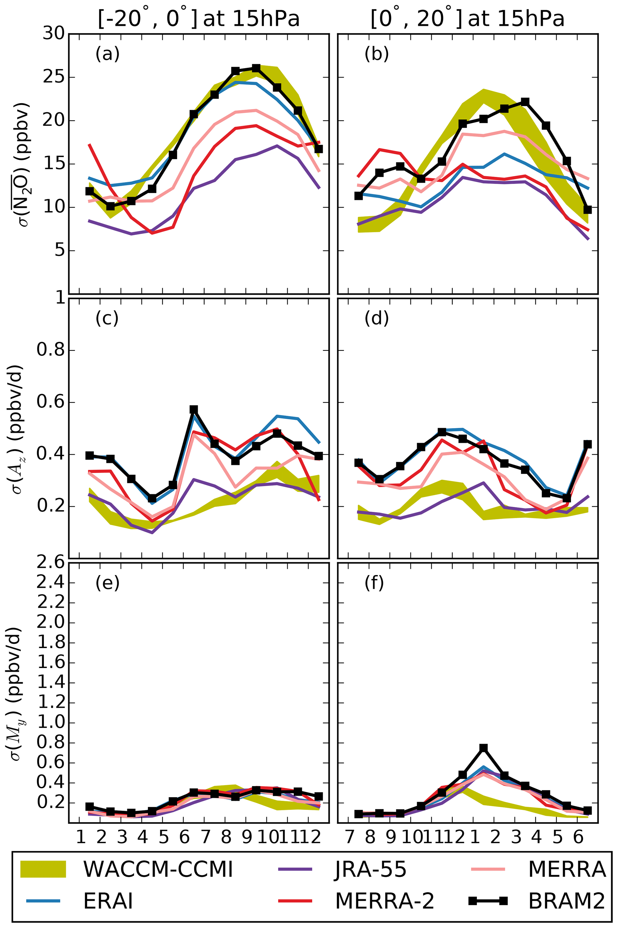
Figure 12As for Fig. 10 but for the tropics: (a, c, e) southern tropics (0–20∘ S); (b, d, f) northern tropics (0–20∘ N).
Figure 12 shows the annual cycles of the standard deviations of the N2O mixing ratio, My and Az for each dataset in the tropical regions (0–20∘ S and N) at 15 hPa for both hemispheres. The interannual variability of the N2O mixing ratio in both the southern and northern tropics depends considerably on the dataset (Fig.12a, b). WACCM-CCMI and the BASCOE reanalysis of the Aura MLS show very similar variabilities, especially in the southern tropics. As the QBO is the major source of variability in the tropical stratosphere (Baldwin et al., 2001), this confirms an earlier comparison that showed a good agreement between the WACCM model and MLS observations in the middle stratosphere in terms of the interannual variability of N2O due to the QBO (Park et al., 2017). Among the CTM simulations, ERAI succeeds at delivering values that are as large as BRAM2 and WACCM-CCMI in the southern tropics, although this is not the case in the northern tropics.
The interannual variability of Az in both hemispheres can be related to the impact of the QBO on the tropical upwelling (Flury et al., 2013). Among MERRA, ERAI and JRA-55, the fraction of variance in deseasonalized tropical upwelling that is associated with the QBO is the largest with ERAI (Abalos et al., 2015). Our findings support this conclusion, as the largest among the reanalyses is again found with ERAI (Fig. 12c, d). However, a detailed analysis of the impact of the QBO on the BDC as illustrated here goes beyond the scope of this study. The variability of My in the tropical regions is small compared with the extra-tropical regions (Fig. 12e, f), which is in agreement with calculations of effective diffusivity that show small variabilities within the tropical pipe (Abalos et al., 2016a). The reanalyses deliver a larger interannual variability in the northern tropics during boreal winter, whereas the variability of My presents a much weaker annual cycle in the southern tropics. WACCM-CCMI does not reproduce this hemispheric asymmetry, with a rather flat profile in both hemispheres and a clear underestimation in the northern tropics, as is also shown for its mean values. In the tropical regions, both the variabilities of My and Az fail to explain the good agreement in the variability of N2O between WACCM and BRAM2, as well as their disagreement with the dynamical reanalyses, because My and Az directly contribute to the N2O tendency rather than its mixing ratio.
We have evaluated the climatological (2005–2014) N2O transport processes in the stratosphere using the tracer continuity equation in the TEM formalism. In particular, we emphasized the horizontal mixing and the vertical advection terms (My and Az, respectively). The upwelling term Az reduces the N2O concentrations in the tropics and increases them in the extra-tropics, whereas My tends to reduce the meridional gradients of N2O and presents large hemispheric differences. As My or Az contribute to the local rates of change of N2O, this analysis is complementary to time-integrated diagnostics such as mAoA. The comparison investigates a variety of datasets, from a free-running chemistry climate model to a reanalysis where dynamics and chemistry are both constrained. The former comprises three realizations of the CCMI REF-C1 experiment by WACCM, and the latter is the chemical reanalysis of Aura MLS driven by ERA-Interim: BRAM2. The intercomparison also includes the BASCOE CTM driven by four dynamical reanalyses – ERAI, JRA-55, MERRA and MERRA-2 – in order to contribute to the S-RIP.
Considering the N2O mixing ratio in the middle stratosphere, all of the datasets agree with respect to the annual cycle, with the large spread in the N2O abundances of the CTM experiments (∼20 %) reflecting the diversity of mAoA obtained with the same model (Chabrillat et al., 2018). The upwelling term Az also agrees among the datasets, especially in the NH where WACCM closely follows the reanalyses. The horizontal mixing term My in the NH is weaker in WACCM compared with the reanalyses. In the extra-tropics, this could be attributed to the weaker forcing from the planetary waves in WACCM compared with the reanalyses. The differences in My become striking in the wintertime Antarctic, where the polar vortex plays a major role. According to the reanalyses, horizontal mixing plays an important role in that region, but that is not found by WACCM. However, this large wintertime My in the reanalyses is challenged by an almost as large residual term. It should be noted that the residual term also includes effects from mixing by diffusion. An additional WACCM run with different gravity waves in the SH is used as a sensitivity test. Over the Antarctic, this test has small impact on My, but it significantly modifies Az in the austral fall and winter due to the enhanced downwelling, and the N2O mixing ratio during spring as a consequence of a more realistic timing of the vortex breakup.
The interannual variability of the mid-stratospheric horizontal mixing term My is largest in the polar regions. It is related to the variability in the vortex breakup dates during spring in the Antarctic, whereas it is related to the highly variable polar vortex in winter in the Arctic. The interannual variability of Az is characterized by a large spread in the mid-stratospheric tropical regions where WACCM-CCMI and JRA-55 deliver a smaller contribution than the other reanalyses. This variability reflects the impact of the QBO on the tropical upwelling (Abalos et al., 2015).
The application of the TEM framework to tracer transport with reanalyses suffers from a poor closure of the budget in the polar regions. We chose to analyze these regions nonetheless, because the differences in My between WACCM and the reanalyses are larger than the residual term, but it remains important to better understand the causes of these large uncertainties. To this end, detailed studies of transport in the polar stratosphere are needed, e.g., comparing the residual circulations with indirect estimates derived from momentum and thermodynamic balances as well as evaluating the effective diffusivity in each dataset (Abalos et al., 2015, 2016a).
The next step of this research consists of the analysis of the interannual variations of the BDC, including the impact of the QBO and the El Niño–Southern Oscillation. Further extensions of this work would include the addition of new reanalysis products such as ERA5 and an intercomparison of several CCMs as already done for the residual circulation itself (Chrysanthou et al., 2019).
The nine monthly climatologies of the N2O mixing ratios and TEM budget terms are freely available at the BIRA-IASB repository (http://repository.aeronomie.be, https://doi.org/10.18758/71021057, Minganti, 2020).
The supplement related to this article is available online at: https://doi.org/10.5194/acp-20-12609-2020-supplement.
DM, SC and EM designed the study. YC provided support with installing and running the models. QE provided the BRAM2 chemical reanalysis and helped with its interpretation. MP ran the CTM experiments. DK provided the WACCM-CCMI realizations and helped with the interpretation of the WACCM datasets. DM wrote and ran the software tools to compute the TEM budgets and realized all of the figures. DM, MA and SC analyzed the TEM budgets. DM and SC wrote the text. All co-authors contributed to the interpretation of the results and the reviews of the drafts of this paper.
The authors declare that they have no conflict of interest.
This article is part of the special issue “The SPARC Reanalysis Intercomparison Project (S-RIP) (ACP/ESSD inter-journal SI)”. It is not associated with a conference.
Emmanuel Mahieu is a research associate with the F.R.S. – FNRS. Marta Abalos acknowledges funding from the Atracción de Talento Comunidad de Madrid (grant no 2016-T2/AMB-1405) and the Spanish National STEADY project (grant no. CGL2017-83198-R). We thank the reanalysis centers (ECMWF, NASA GSFC and JMA) for providing their support and data products. WACCM is a component of NCAR's CESM, which is supported by the NSF and the Office of Science of the U.S. Department of Energy. The authors wish to acknowledge the contribution of Rolando Garcia in the discussion of the paper, specifically regarding the WACCM model results.
This research has been supported by the F.R.S. – FNRS (Brussels) (grant no. PDR.T.0040.16).
This paper was edited by Peter Haynes and reviewed by Mohamadou Diallo and one anonymous referee.
Abalos, M., Randel, W. J., Kinnison, D. E., and Serrano, E.: Quantifying tracer transport in the tropical lower stratosphere using WACCM, Atmos. Chem. Phys., 13, 10591–10607, https://doi.org/10.5194/acp-13-10591-2013, 2013. a, b
Abalos, M., Legras, B., Ploeger, F., and Randel, W. J.: Evaluating the advective Brewer-Dobson circulation in three reanalyses for the period 1979–2012, J. Geophys. Res.-Atmos., 120, 7534–7554, 2015. a, b, c, d, e
Abalos, M., Legras, B., and Shuckburgh, E.: Interannual variability in effective diffusivity in the upper troposphere/lower stratosphere from reanalysis data, Q. J. Roy. Meteorol. Soc., 142, 1847–1861, 2016a. a, b, c
Abalos, M., Randel, W. J., and Birner, T.: Phase-speed spectra of eddy tracer fluxes linked to isentropic stirring and mixing in the upper troposphere and lower stratosphere, J. Atmos. Sci., 73, 4711–4730, 2016b. a
Abalos, M., Randel, W. J., Kinnison, D. E., and Garcia, R. R.: Using the artificial tracer e90 to examine present and future UTLS tracer transport in WACCM, J. Atmos. Sci., 74, 3383–3403, 2017. a, b, c
Andrews, D. G., Holton, J. R., and Leovy, C. B.: Middle atmosphere dynamics, 40, Academic press, USA, 489 pp., 1987. a, b, c, d
Baldwin, M., Gray, L., Dunkerton, T., Hamilton, K., Haynes, P., Randel, W., Holton, J., Alexander, M., Hirota, I., Horinouchi, T., Jones, D. B. A., Kinnersley, J. S., Marquardt, C., Sato, K., and Takahashi, M.: The quasi-biennial oscillation, Rev. Geophys., 39, 179–229, 2001. a, b
Birner, T. and Bönisch, H.: Residual circulation trajectories and transit times into the extratropical lowermost stratosphere, Atmos. Chem. Phys., 11, 817–827, https://doi.org/10.5194/acp-11-817-2011, 2011. a, b
Bönisch, H., Engel, A., Birner, Th., Hoor, P., Tarasick, D. W., and Ray, E. A.: On the structural changes in the Brewer-Dobson circulation after 2000, Atmos. Chem. Phys., 11, 3937–3948, https://doi.org/10.5194/acp-11-3937-2011, 2011. a
Brasseur, G. P. and Solomon, S.: Aeronomy of the middle atmosphere: chemistry and physics of the stratosphere and mesosphere, Vol. 32, Springer Science & Business Media, the Netherlands, 637 pp., 2006. a
Brewer, A.: Evidence for a world circulation provided by the measurements of helium and water vapour distribution in the stratosphere, Q. J. Roy. Meteorol. Soc., 75, 351–363, 1949. a
Butchart, N.: The Brewer-Dobson circulation, Rev. Geophys., 52, 157–184, 2014. a, b, c
Butchart, N., Cionni, I., Eyring, V., Shepherd, T., Waugh, D., Akiyoshi, H., Austin, J., Brühl, C., Chipperfield, M., Cordero, E., Dameris, M., Deckert, R., Dhomse, S., Frith, S. M., Garcia, R. R., Gettelman, A., Giorgetta, M. A., Kinnison, D. E., Li, F., Mancini, E., Mclandress, C., Pawson, S., Pitari, G., Plummer, D. A., Rozanov, E., Sassi, F., Scinocca, J. F., Shibata, K., Steil, B., and Tian, W.: Chemistry–climate model simulations of twenty-first century stratospheric climate and circulation changes, J. Clim., 23, 5349–5374, 2010. a
Butler, A. H., Sjoberg, J. P., Seidel, D. J., and Rosenlof, K. H.: A sudden stratospheric warming compendium, Earth Syst. Sci. Data, 9, 63–76, https://doi.org/10.5194/essd-9-63-2017, 2017. a, b
Cameron, C., Bodeker, G. E., Conway, J. P., Stuart, S., and Renwick, J.: Simulating the Antarctic stratospheric vortex transport barrier: comparing the Unified Model to reanalysis, Clim. Dynam., 53, 441–452, 2019. a
Chabrillat, S., Vigouroux, C., Christophe, Y., Engel, A., Errera, Q., Minganti, D., Monge-Sanz, B. M., Segers, A., and Mahieu, E.: Comparison of mean age of air in five reanalyses using the BASCOE transport model, Atmos. Chem. Phys., 18, 14715–14735, https://doi.org/10.5194/acp-18-14715-2018, 2018. a, b, c, d, e, f, g, h, i, j, k, l
Charney, J. G. and Drazin, P. G.: Propagation of planetary-scale disturbances from the lower into the upper atmosphere, J. Geophys. Res., 66, 83–109, 1961. a
Chipperfield, M. P.: New version of the TOMCAT/SLIMCAT off-line chemical transport model: Intercomparison of stratospheric tracer experiments, Q. J. Roy. Meteorol. Soc., 132, 1179–1203, https://doi.org/10.1256/qj.05.51, 2006. a
Chrysanthou, A., Maycock, A. C., Chipperfield, M. P., Dhomse, S., Garny, H., Kinnison, D., Akiyoshi, H., Deushi, M., Garcia, R. R., Jöckel, P., Kirner, O., Pitari, G., Plummer, D. A., Revell, L., Rozanov, E., Stenke, A., Tanaka, T. Y., Visioni, D., and Yamashita, Y.: The effect of atmospheric nudging on the stratospheric residual circulation in chemistry–climate models, Atmos. Chem. Phys., 19, 11559–11586, https://doi.org/10.5194/acp-19-11559-2019, 2019. a
Conley, A. J., Garcia, R., Kinnison, D., Lamarque, J.-F., Marsh, D., Mills, M., Smith, A. K., Tilmes, S., Vitt, F., Morrison, H., Cameron-Smith, P., Collins, W. D., Iacono, M. J., Easter, R. C., Ghan, S. I., Liu, X., Rasch, P. J., and Taylor, M. A.: Description of the NCAR community atmosphere model (CAM 5.0), NCAR Technical note, 254 pp., 2012. a
Davis, S. M., Rosenlof, K. H., Hassler, B., Hurst, D. F., Read, W. G., Vömel, H., Selkirk, H., Fujiwara, M., and Damadeo, R.: The Stratospheric Water and Ozone Satellite Homogenized (SWOOSH) database: a long-term database for climate studies, Earth Syst. Sci. Data, 8, 461–490, https://doi.org/10.5194/essd-8-461-2016, 2016. a
de la Cámara, A., Mechoso, C. R., Mancho, A. M., Serrano, E., and Ide, K.: Isentropic Transport within the Antarctic Polar-Night Vortex: Rossby Wave Breaking Evidence and Lagrangian Structures, J. Atmos. Sci., 70, 2982–3001, https://doi.org/10.1175/JAS-D-12-0274.1, 2013. a
Dee, D. P., Uppala, S., Simmons, A., Berrisford, P., Poli, P., Kobayashi, S., Andrae, U., Balmaseda, M., Balsamo, G., Bauer, P., Bechtold, P., Beljaars, A. C. M., van de Berg, L., Bidlot, J., Bormann, N., Delsol, C., Dragani, R., Fuentes, M., Geer, A. J., Haimberger, L., Healy, S. B., Hersbach, H., Holm, E. V., Isaksen, L., Källberg, P., Köhler, M., Matricardi, M., McNally, A. P., Monge-Sanz, B. M., Morcrette, J.-J., Park, B.-K., Peubey, C., de Rosnay, P., Tavolato, C., Thepaut, J.-N., and Vitarta, F.: The ERA-Interim reanalysis: Configuration and performance of the data assimilation system, Q. J. Roy. Meteorol. Soc., 137, 553–597, 2011. a, b, c, d, e
Diallo, M., Legras, B., and Chédin, A.: Age of stratospheric air in the ERA-Interim, Atmos. Chem. Phys., 12, 12133–12154, https://doi.org/10.5194/acp-12-12133-2012, 2012. a
Diallo, M., Riese, M., Birner, T., Konopka, P., Müller, R., Hegglin, M. I., Santee, M. L., Baldwin, M., Legras, B., and Ploeger, F.: Response of stratospheric water vapor and ozone to the unusual timing of El Niño and the QBO disruption in 2015–2016, Atmos. Chem. Phys., 18, 13055–13073, https://doi.org/10.5194/acp-18-13055-2018, 2018. a
Diallo, M., Konopka, P., Santee, M. L., Müller, R., Tao, M., Walker, K. A., Legras, B., Riese, M., Ern, M., and Ploeger, F.: Structural changes in the shallow and transition branch of the Brewer–Dobson circulation induced by El Niño, Atmos. Chem. Phys., 19, 425–446, https://doi.org/10.5194/acp-19-425-2019, 2019. a
Dietmüller, S., Garny, H., Plöger, F., Jöckel, P., and Cai, D.: Effects of mixing on resolved and unresolved scales on stratospheric age of air, Atmos. Chem. Phys., 17, 7703–7719, https://doi.org/10.5194/acp-17-7703-2017, 2017. a, b
Dietmüller, S., Eichinger, R., Garny, H., Birner, T., Boenisch, H., Pitari, G., Mancini, E., Visioni, D., Stenke, A., Revell, L., Rozanov, E., Plummer, D. A., Scinocca, J., Jöckel, P., Oman, L., Deushi, M., Kiyotaka, S., Kinnison, D. E., Garcia, R., Morgenstern, O., Zeng, G., Stone, K. A., and Schofield, R.: Quantifying the effect of mixing on the mean age of air in CCMVal-2 and CCMI-1 models, Atmos. Chem. Phys., 18, 6699–6720, https://doi.org/10.5194/acp-18-6699-2018, 2018. a, b, c
Dobson, G. M. B.: Origin and distribution of the polyatomic molecules in the atmosphere, Proc. Roy. Soc. London Ser. A, 236, 187–193, 1956. a
Dobson, G. M. B., Harrison, D., and Lawrence, J.: Measurements of the amount of ozone in the Earth's atmosphere and its relation to other geophysical conditions – Part III, Proc. Roy. Soc. London Ser. A, 122, 456–486, 1929. a
Edmon, H., Hoskins, B., and McIntyre, M.: Eliassen-Palm cross sections for the troposphere, J. Atmos. Sci., 37, 2600–2616, 1980. a
Engel, A., Möbius, T., Bönisch, H., Schmidt, U., Heinz, R., Levin, I., Atlas, E., Aoki, S., Nakazawa, T., Sugawara, S., Moore, F., Hurst, D., Elkins, J., Schauffler, S., Andrews, A., and Boering, K.: Age of stratospheric air unchanged within uncertainties over the past 30 years, Nat. Geosci., 2, 28–31, 2009. a
Engel, A., Bönisch, H., Ullrich, M., Sitals, R., Membrive, O., Danis, F., and Crevoisier, C.: Mean age of stratospheric air derived from AirCore observations, Atmos. Chem. Phys., 17, 6825–6838, https://doi.org/10.5194/acp-17-6825-2017, 2017. a
Errera, Q., Daerden, F., Chabrillat, S., Lambert, J. C., Lahoz, W. A., Viscardy, S., Bonjean, S., and Fonteyn, D.: 4D-Var assimilation of MIPAS chemical observations: ozone and nitrogen dioxide analyses, Atmos. Chem. Phys., 8, 6169-6187, https://doi.org/10.5194/acp-8-6169-2008, 2008. a
Errera, Q., Chabrillat, S., Christophe, Y., Debosscher, J., Hubert, D., Lahoz, W., Santee, M. L., Shiotani, M., Skachko, S., von Clarmann, T., and Walker, K.: Technical note: Reanalysis of Aura MLS chemical observations, Atmos. Chem. Phys., 19, 13647–13679, https://doi.org/10.5194/acp-19-13647-2019, 2019. a, b, c, d, e, f, g
Flury, T., Wu, D. L., and Read, W. G.: Variability in the speed of the Brewer–Dobson circulation as observed by Aura/MLS, Atmos. Chem. Phys., 13, 4563–4575, https://doi.org/10.5194/acp-13-4563-2013, 2013. a
Fritsch, F., Garny, H., Engel, A., Bönisch, H., and Eichinger, R.: Sensitivity of age of air trends to the derivation method for non-linear increasing inert SF6, Atmos. Chem. Phys., 20, 8709–8725, https://doi.org/10.5194/acp-20-8709-2020, 2020. a
Froidevaux, L., Kinnison, D. E., Wang, R., Anderson, J., and Fuller, R. A.: Evaluation of CESM1 (WACCM) free-running and specified dynamics atmospheric composition simulations using global multispecies satellite data records, Atmos. Chem. Phys., 19, 4783–4821, https://doi.org/10.5194/acp-19-4783-2019, 2019. a, b, c
Fueglistaler, S., Dessler, A., Dunkerton, T., Folkins, I., Fu, Q., and Mote, P. W.: Tropical tropopause layer, Rev. Geophys., 47, RG1004, https://doi.org/10.1029/2008RG000267, 2009. a
Fujiwara, M., Wright, J. S., Manney, G. L., Gray, L. J., Anstey, J., Birner, T., Davis, S., Gerber, E. P., Harvey, V. L., Hegglin, M. I., Homeyer, C. R., Knox, J. A., Krüger, K., Lambert, A., Long, C. S., Martineau, P., Molod, A., Monge-Sanz, B. M., Santee, M. L., Tegtmeier, S., Chabrillat, S., Tan, D. G. H., Jackson, D. R., Polavarapu, S., Compo, G. P., Dragani, R., Ebisuzaki, W., Harada, Y., Kobayashi, C., McCarty, W., Onogi, K., Pawson, S., Simmons, A., Wargan, K., Whitaker, J. S., and Zou, C.-Z.: Introduction to the SPARC Reanalysis Intercomparison Project (S-RIP) and overview of the reanalysis systems, Atmos. Chem. Phys., 17, 1417–1452, https://doi.org/10.5194/acp-17-1417-2017, 2017. a, b, c, d
Galytska, E., Rozanov, A., Chipperfield, M. P., Dhomse, Weber, M., Arosio, C., Feng, W., and Burrows, J. P.: Dynamically controlled ozone decline in the tropical mid-stratosphere observed by SCIAMACHY, Atmos. Chem. Phys., 19, 767–783, https://doi.org/10.5194/acp-19-767-2019, 2019. a
Garcia, R. R., Randel, W. J., and Kinnison, D. E.: On the determination of age of air trends from atmospheric trace species, J. Atmos. Sci., 68, 139–154, 2011. a
Garcia, R. R., Smith, A. K., Kinnison, D. E., Cámara, Á. d. l., and Murphy, D. J.: Modification of the gravity wave parameterization in the Whole Atmosphere Community Climate Model: Motivation and results, J. Atmos. Sci., 74, 275–291, 2017. a, b, c, d, e, f, g, h, i
Gelaro, R., McCarty, W., Suárez, M. J., Todling, R., Molod, A., Takacs, L., Randles, C. A., Darmenov, A., Bosilovich, M. G., Reichle, R., Wargan, K., Coy, L., Cullather, R., Draper, C., Akella, S., Buchard, V., Conaty, A., da Silva, A. M., Gu, W., Kim, G.-K., Koster, R., Lucchesi, R., Merkova, D., Nielsen, J. E., Partyka, G., Pawson, S., Putman, W., Rienecker, M., Schubert, S. D., Sienkiewicz, M., and Zhao, B.: The modern-era retrospective analysis for research and applications, version 2 (MERRA-2), J. Clim., 30, 5419–5454, 2017. a, b, c, d
Gerber, E. P.: Stratospheric versus tropospheric control of the strength and structure of the Brewer–Dobson circulation, J. Atmos. Sci., 69, 2857–2877, 2012. a
Gerber, E. P., Baldwin, M. P., Akiyoshi, H., Austin, J., Bekki, S., Braesicke, P., Butchart, N., Chipperfield, M., Dameris, M., Dhomse, S., Frith, S. M., Garcia, R. R., Garny, H., Getterlman, A., Hardiman, S. C., Karpechko, A., Marchand, M., Morgenstern, O., Nielsen, J. E., Pawson, S., Peter, T., Plummer, D. A., Pyle, J. A., Rozanov, E., Scinnocca, J. F., Shepherd, T. G., and Smale, D.: Stratosphere-troposphere coupling and annular mode variability in chemistry-climate models, J. Geophys. Res.-Atmos., 115, D00M06, https://doi.org/10.1029/2009JD013770, 2010. a
Haenel, F. J., Stiller, G. P., von Clarmann, T., Funke, B., Eckert, E., Glatthor, N., Grabowski, U., Kellmann, S., Kiefer, M., Linden, A., and Reddmann, T.: Reassessment of MIPAS age of air trends and variability, Atmos. Chem. Phys., 15, 13161–13176, https://doi.org/10.5194/acp-15-13161-2015, 2015. a
Hall, T. M., Waugh, D. W., Boering, K. A., and Plumb, R. A.: Evaluation of transport in stratospheric models, J. Geophys. Res.-Atmos., 104, 18815–18839, 1999. a
Hardiman, S. C., Butchart, N., and Calvo, N.: The morphology of the Brewer–Dobson circulation and its response to climate change in CMIP5 simulations, Q. J. Roy. Meteorol. Soc., 140, 1958–1965, 2014. a
Hardiman, S. C., Lin, P., Scaife, A. A., Dunstone, N. J., and Ren, H.-L.: The influence of dynamical variability on the observed Brewer-Dobson circulation trend, Geophys. Res. Lett., 44, 2885–2892, 2017. a, b
Haynes, P. and Shuckburgh, E.: Effective diffusivity as a diagnostic of atmospheric transport: 2. Troposphere and lower stratosphere, J. Geophys. Res.-Atmos., 105, 22795–22810, 2000. a
Haynes, P., McIntyre, M., Shepherd, T., Marks, C., and Shine, K. P.: On the downward control of extratropical diabatic circulations by eddy-induced mean zonal forces, J. Atmos. Sci.s, 48, 651–678, 1991. a
Hegglin, M., Plummer, D., Shepherd, T., Scinocca, J., Anderson, J., Froidevaux, L., Funke, B., Hurst, D., Rozanov, A., Urban, J., von Clarmann, T., Walker, K. A., Wang, H. J., Tegtmeier, S., and Weigel, K.: Vertical structure of stratospheric water vapour trends derived from merged satellite data, Nat. Geosci., 7, 768–776, 2014. a
Holton, J.: An Introduction to Dynamic Meteorology, no. v. 1 in An Introduction to Dynamic Meteorology, Elsevier Science, available at: https://books.google.be/books?id=fhW5oDv3EPsC (last access: 28 October 2020), 2004. a, b
Hurrell, J. W., Holland, M. M., Gent, P. R., Ghan, S., Kay, J. E., Kushner, P. J., Lamarque, J.-F., Large, W. G., Lawrence, D., Lindsay, K., Lipscomb, W. H., Long, M. C., Mahowald, N., Marsh, D. R., Neale, R. B., Rasch, P., Vavrus, S., Vertenstein, M., Bader, D., Collins, W. D., Hack, J. J., Kiehl, J., and Marshall, S.: The community earth system model: a framework for collaborative research, B. Am. Meteorol. Soc., 94, 1339–1360, 2013. a
Kawatani, Y., Hamilton, K., Miyazaki, K., Fujiwara, M., and Anstey, J. A.: Representation of the tropical stratospheric zonal wind in global atmospheric reanalyses, Atmos. Chem. Phys., 16, 6681–6699, https://doi.org/10.5194/acp-16-6681-2016, 2016. a
Kidston, J., Scaife, A. A., Hardiman, S. C., Mitchell, D. M., Butchart, N., Baldwin, M. P., and Gray, L. J.: Stratospheric influence on tropospheric jet streams, storm tracks and surface weather, Nat. Geosci., 8, 433–440, 2015. a
Kinnison, D., Brasseur, G., Walters, S., Garcia, R., Marsh, D., Sassi, F., Harvey, V., Randall, C., Emmons, L., Lamarque, J.-F., Hess, P., Orlando, J. J., Tie, X. X., Randel, W., Pan, L. L., Gettelman, A., Granier, C., Diehl, T., Niemeier, U., and Simmons, A. J.: Sensitivity of chemical tracers to meteorological parameters in the MOZART-3 chemical transport model, J. Geophys. Res.-Atmos., 112, D20302, https://doi.org/10.1029/2006JD007879, 2007. a
Kobayashi, S., Ota, Y., Harada, Y., Ebita, A., Moriya, M., Onoda, H., Onogi, K., Kamahori, H., Kobayashi, C., Endo, H., Miyaoka, K., and Takahashi, K.: The JRA-55 reanalysis: General specifications and basic characteristics, J. Meteorol. Soc. Jpn. Ser. II, 93, 5–48, 2015. a, b, c, d
Konopka, P., Grooß, J.-U., Günther, G., Ploeger, F., Pommrich, R., Müller, R., and Livesey, N.: Annual cycle of ozone at and above the tropical tropopause: observations versus simulations with the Chemical Lagrangian Model of the Stratosphere (CLaMS), Atmos. Chem. Phys., 10, 121–132, https://doi.org/10.5194/acp-10-121-2010, 2010. a
Konopka, P., Ploeger, F., Tao, M., Birner, T., and Riese, M.: Hemispheric asymmetries and seasonality of mean age of air in the lower stratosphere: Deep versus shallow branch of the Brewer-Dobson circulation, J. Geophys. Res.-Atmos., 120, 2053–2066, 2015. a, b, c
Lahoz, W. and Errera, Q.: Data Assimilation: Making Sense of Observations, Constituent Assimilation, Springer, Berlin, Heideberg, 449–490, 2010. a
Lean, J., Rottman, G., Harder, J., and Kopp, G.: SORCE contributions to new understanding of global change and solar variability, in: The Solar Radiation and Climate Experiment (SORCE), Springer, New York, NY, 27–53, 2005. a
Li, F., Waugh, D. W., Douglass, A. R., Newman, P. A., Pawson, S., Stolarski, R. S., Strahan, S. E., and Nielsen, J. E.: Seasonal variations of stratospheric age spectra in the Goddard Earth Observing System Chemistry Climate Model (GEOSCCM), J. Geophys. Res.-Atmos., 117, D5, https://doi.org/10.1029/2011JD016877, 2012. a
Lin, P. and Fu, Q.: Changes in various branches of the Brewer–Dobson circulation from an ensemble of chemistry climate models, J. Geophys. Res.-Atmos., 118, 73–84, 2013. a
Lin, S.-J.: A “vertically Lagrangian” finite-volume dynamical core for global models, Mon. Weather Rev., 132, 2293–2307, 2004. a, b
Lin, S.-J. and Rood, R. B.: Multidimensional flux-form semi-Lagrangian transport schemes, Mon. Weather Rev., 124, 2046–2070, 1996. a
Livesey, N., Read, W., Wagner, P., Froidevaux, L., Lambert, A., Manney, G., Pumphrey, H., Santee, M., Schwartz, M., Wang, S., Fuller, R. A., Jarnot, R. F., Knosp, B. W., and Martinez, E.: Earth Observing System (EOS) Aura Microwave Limb Sounder (MLS) version 4.2x level 2 data quality and description document, JPL D-33509 rev. A, A, JPL publication, Pasadena, CA, USA, 174 pp., 2015. a, b
Long, C. S., Fujiwara, M., Davis, S., Mitchell, D. M., and Wright, C. J.: Climatology and interannual variability of dynamic variables in multiple reanalyses evaluated by the SPARC Reanalysis Intercomparison Project (S-RIP), Atmos. Chem. Phys., 17, 14593–14629, https://doi.org/10.5194/acp-17-14593-2017, 2017. a
Mahieu, E., Chipperfield, M., Notholt, J., Reddmann, T., Anderson, J., Bernath, P., Blumenstock, T., Coffey, M., Dhomse, S., Feng, W., Franco, B., Froidevaux, L., Griffith, D. W. T., Hannigan, J. W., Hase, F., Hossaini, R., Jones, N. B., Morino, I., Murata, I., Nakajima, H., Palm, M., Paton-Walsh, C., Russell III, J. M., Schneider, M., Servais, C., Smale, D., and Walker, K. A.: Recent Northern Hemisphere stratospheric HCl increase due to atmospheric circulation changes, Nature, 515, 104–107, 2014. a
Manney, G. L., Sabutis, J. L., Pawson, S., Santee, M. L., Naujokat, B., Swinbank, R., Gelman, M. E., and Ebisuzaki, W.: Lower stratospheric temperature differences between meteorological analyses in two cold Arctic winters and their impact on polar processing studies, J. Geophys. Res.-Atmos., 108, 8328, https://doi.org/10.1029/2001JD001149, 2003. a
Marsh, D. R., Mills, M. J., Kinnison, D. E., Lamarque, J.-F., Calvo, N., and Polvani, L. M.: Climate change from 1850 to 2005 simulated in CESM1 (WACCM), J. Clim., 26, 7372–7391, 2013. a, b, c
Matthes, K., Marsh, D. R., Garcia, R. R., Kinnison, D. E., Sassi, F., and Walters, S.: Role of the QBO in modulating the influence of the 11 year solar cycle on the atmosphere using constant forcings, J. Geophys. Res.-Atmos., 115, D18110, https://doi.org/10.1029/2009JD013020, 2010. a
McIntyre, M. E. and Palmer, T.: Breaking planetary waves in the stratosphere, Nature, 305, 593–600, 1983. a
Ménard, R., Chabrillat, S., Robichaud, A., de Grandpré, J., Charron, M., Rochon, Y., Batchelor, R., Kallaur, A., Reszka, M., and Kaminski, J.: Coupled Stratospheric Chemistry-Meteorology Data Assimilation, Part I: Physical Background and Coupled Modeling Aspects, Atmosphere, 11, 150, https://doi.org/10.3390/atmos11020150, 2020. a
Minganti, D.: Supplement for: Climatological impact of the Brewer-Dobson Circulation on the N2O budget in WACCM, a chemical reanalysis and a CTM driven by four dynamical reanalyses, https://doi.org/10.18758/71021057, 2020.
Miyazaki, K. and Iwasaki, T.: Diagnosis of meridional ozone transport based on mass-weighted isentropic zonal means, J. Atmos. Sci., 62, 1192–1208, 2005. a
Monge-Sanz, B. M., Chipperfield, M. P., Dee, D. P., Simmons, A. J., and Uppala, S. M.: Improvements in the stratospheric transport achieved by a chemistry transport model with ECMWF (re)analyses: identifying effects and remaining challenges, Q. J. Roy. Meteorol. Soc., 139, 654–673, https://doi.org/10.1002/qj.1996, 2012. a
Morgenstern, O., Hegglin, M. I., Rozanov, E., O'Connor, F. M., Abraham, N. L., Akiyoshi, H., Archibald, A. T., Bekki, S., Butchart, N., Chipperfield, M. P., Deushi, M., Dhomse, S. S., Garcia, R. R., Hardiman, S. C., Horowitz, L. W., Jöckel, P., Josse, B., Kinnison, D., Lin, M., Mancini, E., Manyin, M. E., Marchand, M., Marécal, V., Michou, M., Oman, L. D., Pitari, G., Plummer, D. A., Revell, L. E., Saint-Martin, D., Schofield, R., Stenke, A., Stone, K., Sudo, K., Tanaka, T. Y., Tilmes, S., Yamashita, Y., Yoshida, K., and Zeng, G.: Review of the global models used within phase 1 of the Chemistry–Climate Model Initiative (CCMI), Geosci. Model Dev., 10, 639–671, https://doi.org/10.5194/gmd-10-639-2017, 2017. a
Neale, R. B., Richter, J., Park, S., Lauritzen, P. H., Vavrus, S. J., Rasch, P. J., and Zhang, M.: The mean climate of the Community Atmosphere Model (CAM4) in forced SST and fully coupled experiments, J. Clim., 26, 5150–5168, 2013. a
Newman, P. A. and Nash, E. R.: Quantifying the wave driving of the stratosphere, J. Geophys. Res.-Atmos., 105, 12485–12497, 2000. a
Newman, P. A. and Nash, E. R.: The unusual Southern Hemisphere stratosphere winter of 2002, J. Atmos. Sci., 62, 614–628, 2005. a
Palmeiro, F. M., Calvo, N., and Garcia, R. R.: Future changes in the Brewer–Dobson circulation under different greenhouse gas concentrations in WACCM4, J. Atmos. Sci., 71, 2962–2975, 2014. a
Park, M., Randel, W., Kinnison, D., Bourassa, A., Degenstein, D., Roth, C., McLinden, C., Sioris, C., Livesey, N., and Santee, M.: Variability of stratospheric reactive nitrogen and ozone related to the QBO, J. Geophys. Res.-Atmos., 122, 10–103, 2017. a
Ploeger, F. and Birner, T.: Seasonal and inter-annual variability of lower stratospheric age of air spectra, Atmos. Chem. Phys., 16, 10195–10213, https://doi.org/10.5194/acp-16-10195-2016, 2016. a
Ploeger, F., Legras, B., Charlesworth, E., Yan, X., Diallo, M., Konopka, P., Birner, T., Tao, M., Engel, A., and Riese, M.: How robust are stratospheric age of air trends from different reanalyses?, Atmos. Chem. Phys., 19, 6085–6105, https://doi.org/10.5194/acp-19-6085-2019, 2019. a
Plumb, R. A.: Stratospheric transport, J. Meteorol. Soc. Jpn. Ser. II, 80, 793–809, 2002. a, b, c
Polvani, L. M., Abalos, M., Garcia, R., Kinnison, D., and Randel, W. J.: Significant Weakening of Brewer-Dobson Circulation Trends Over the 21st Century as a Consequence of the Montreal Protocol, Geophys. Res. Lett., 45, 401–409, 2018. a
Prignon, M., Chabrillat, S., Minganti, D., O'Doherty, S., Servais, C., Stiller, G., Toon, G. C., Vollmer, M. K., and Mahieu, E.: Improved FTIR retrieval strategy for HCFC-22 (CHClF2), comparisons with in situ and satellite datasets with the support of models, and determination of its long-term trend above Jungfraujoch, Atmos. Chem. Phys., 19, 12309–12324, https://doi.org/10.5194/acp-19-12309-2019, 2019. a, b
Randel, W. J. and Newman, P. A.: The stratosphere in the Southern Hemisphere, in: Meteorology of the Southern Hemisphere, Springer, Boston, MA, 243–282, 1998. a, b
Randel, W. J., Boville, B. A., Gille, J. C., Bailey, P. L., Massie, S. T., Kumer, J., Mergenthaler, J., and Roche, A.: Simulation of stratospheric N2O in the NCAR CCM2: Comparison with CLAES data and global budget analyses, Journal of the atmospheric sciences, 51, 2834–2845, 1994. a, b, c
Rao, J., Ren, R., and Yang, Y.: Parallel comparison of the northern winter stratospheric circulation in reanalysis and in CMIP5 models, Adv. Atmos. Sci., 32, 952–966, 2015. a
Richter, J. H., Sassi, F., and Garcia, R. R.: Toward a physically based gravity wave source parameterization in a general circulation model, J. Atmos. Sci., 67, 136–156, 2010. a
Rienecker, M. M., Suarez, M. J., Gelaro, R., Todling, R., Bacmeister, J., Liu, E., Bosilovich, M. G., Schubert, S. D., Takacs, L., Kim, G.-K., Bloom, S., Junye, C., Collins, D., Conaty, A., da Silva, A., Gu, W., Joiner, J., Koster, R. D., Lucchesi, R., Molod, A., Owens, T., Pawson, S., Pegion, P., Redder, C. R., Reichle, R., Robertson, F. R., Ruddick, A. G., Sienkiewicz, M., and Woollen, J.: MERRA: NASA' modern-era retrospective analysis for research and applications, J. Clim., 24, 3624–3648, 2011. a, b, c, d
Riese, M., Ploeger, F., Rap, A., Vogel, B., Konopka, P., Dameris, M., and Forster, P.: Impact of uncertainties in atmospheric mixing on simulated UTLS composition and related radiative effects, J. Geophys. Res.-Atmos., 117, D16305, https://doi.org/10.1029/2012JD017751, 2012. a
Roscoe, H. K., Feng, W., Chipperfield, M. P., Trainic, M., and Shuckburgh, E. F.: The existence of the edge region of the Antarctic stratospheric vortex, J. Geophys. Res.-Atmos., 117, D04301, https://doi.org/10.1029/2011JD015940, 2012. a
Rosenlof, K. H. and Holton, J. R.: Estimates of the stratospheric residual circulation using the downward control principle, J. Geophys. Res.-Atmos., 98, 10465–10479, 1993. a
Salby, M. L. and Callaghan, P. F.: Interaction between the Brewer–Dobson circulation and the Hadley circulation, J. Clim., 18, 4303–4316, 2005. a
Sato, K. and Hirano, S.: The climatology of the Brewer–Dobson circulation and the contribution of gravity waves, Atmos. Chem. Phys., 19, 4517–4539, https://doi.org/10.5194/acp-19-4517-2019, 2019. a
Scaife, A. and James, I.: Response of the stratosphere to interannual variability of tropospheric planetary waves, Q. J. Roy. Meteorol. Soc., 126, 275–297, 2000. a
Schoeberl, M., Douglass, A., Stolarski, R., Pawson, S., Strahan, S., and Read, W.: Comparison of lower stratospheric tropical mean vertical velocities, J. Geophys. Res.-Atmos., 113, D24109, https://doi.org/10.1029/2008JD010221, 2008. a
Seinfeld, J. H. and Pandis, S. N.: Atmospheric chemistry and physics: from air pollution to climate change, John Wiley & Sons, 1152 pp., 2016. a
Shepherd, T. G.: Transport in the middle atmosphere, J. Meteorol. Soc. Jpn. Ser. II, 85, 165–191, 2007. a, b
Solomon, S., Kinnison, D., Bandoro, J., and Garcia, R.: Simulation of polar ozone depletion: An update, J. Geophys. Res.-Atmos., 120, 7958–7974, 2015. a
Stiller, G. P., von Clarmann, T., Haenel, F., Funke, B., Glatthor, N., Grabowski, U., Kellmann, S., Kiefer, M., Linden, A., Lossow, S., and López-Puertas, M.: Observed temporal evolution of global mean age of stratospheric air for the 2002 to 2010 period, Atmos. Chem. Phys., 12, 3311–3331, https://doi.org/10.5194/acp-12-3311-2012, 2012. a
Strahan, S., Oman, L., Douglass, A., and Coy, L.: Modulation of Antarctic vortex composition by the quasi-biennial oscillation, Geophys. Res. Lett., 42, 4216–4223, 2015. a, b
Strahan, S. E., Douglass, A., Stolarski, R., Akiyoshi, H., Bekki, S., Braesicke, P., Butchart, N., Chipperfield, M., Cugnet, D., Dhomse, S., Frith, S. M., Gettelman, A., Hardiman, S. C., Kinnison, D. E., Lamarque, J. F., Mancini, E., Marchand, M., Michou, M., Morgenstern, O., Nakamura, T., Olivie, D., Pawson, S., Pitari, G., Plummer, D. A., Pyle, J. A., Scinocca, J. F., Shepherd, T. G., Shibata, K., Smale, D., Teyssedre, H., Tian, W., and Yamashita, Y.: Using transport diagnostics to understand chemistry climate model ozone simulations, J. Geophys. Res.-Atmos., 116, D17302, https://doi.org/10.1029/2010JD015360, 2011. a
Tao, M., Konopka, P., Ploeger, F., Yan, X., Wright, J. S., Diallo, M., Fueglistaler, S., and Riese, M.: Multitimescale variations in modeled stratospheric water vapor derived from three modern reanalysis products, Atmos. Chem. Phys., 19, 6509–6534, https://doi.org/10.5194/acp-19-6509-2019, 2019. a
Tweedy, O., Waugh, D., Stolarski, R., Oman, L. D., Randel, W., and Abalos, M.: Hemispheric differences in the annual cycle of tropical lower stratosphere transport and tracers, J. Geophys. Res.-Atmos., 122, 7183–7199, 2017. a, b, c, d
Waugh, D. and Hall, T.: Age of stratospheric air: Theory, observations, and models, Rev. Geophys., 40, 1–1010, 2002. a
Waugh, D. W. and Randel, W. J.: Climatology of Arctic and Antarctic polar vortices using elliptical diagnostics, J. Atmos. Sci., 56, 1594–1613, 1999. a, b, c
Yamazaki, Y., Matthias, V., Miyoshi, Y., Stolle, C., Siddiqui, T., Kervalishvili, G., Laštovička, J., Kozubek, M., Ward, W., Themens, D. R., Kristoffersen, S., and Alken, P.: September 2019 Antarctic sudden stratospheric warming: quasi-6-day wave burst and ionospheric effects, Geophys. Res. Lette., 47, e2019GL086577, https://doi.org/10.1029/2019GL086577, 2019. a
Yang, H., Chen, G., and Domeisen, D. I.: Sensitivities of the lower-stratospheric transport and mixing to tropical SST heating, J. Atmos. Sci., 71, 2674–2694, 2014. a
- Abstract
- Introduction
- Data and method
- Latitude–pressure cross sections
- Climatological seasonal cycles
- Interannual variability of the seasonal cycles
- Summary and conclusions
- Data availability
- Author contributions
- Competing interests
- Special issue statement
- Acknowledgements
- Financial support
- Review statement
- References
- Supplement