the Creative Commons Attribution 4.0 License.
the Creative Commons Attribution 4.0 License.
 | 31 Oct 2020
Polar stratospheric clouds initiated by mountain waves in a global chemistry–climate model: a missing piece in fully modelling polar stratospheric ozone depletion
Andrew Orr
J. Scott Hosking
Aymeric Delon
Lars Hoffmann
Reinhold Spang
Tracy Moffat-Griffin
James Keeble
Nathan Luke Abraham
Peter Braesicke
An important source of polar stratospheric clouds (PSCs), which play a crucial role in controlling polar stratospheric ozone depletion, is the temperature fluctuations induced by mountain waves. These enable stratospheric temperatures to fall below the threshold value for PSC formation in regions of negative temperature perturbations or cooling phases induced by the waves even if the synoptic-scale temperatures are too high. However, this formation mechanism is usually missing in global chemistry–climate models because these temperature fluctuations are neither resolved nor parameterised. Here, we investigate in detail the episodic and localised wintertime stratospheric cooling events produced over the Antarctic Peninsula by a parameterisation of mountain-wave-induced temperature fluctuations inserted into a 30-year run of the global chemistry–climate configuration of the UM-UKCA (Unified Model – United Kingdom Chemistry and Aerosol) model. Comparison of the probability distribution of the parameterised cooling phases with those derived from climatologies of satellite-derived AIRS brightness temperature measurements and high-resolution radiosonde temperature soundings from Rothera Research Station on the Antarctic Peninsula shows that they broadly agree with the AIRS observations and agree well with the radiosonde observations, particularly in both cases for the “cold tails” of the distributions. It is further shown that adding the parameterised cooling phase to the resolved and synoptic-scale temperatures in the UM-UKCA model results in a considerable increase in the number of instances when minimum temperatures fall below the formation temperature for PSCs made from ice water during late austral autumn and early austral winter and early austral spring, and without the additional cooling phase the temperature rarely falls below the ice frost point temperature above the Antarctic Peninsula in the model. Similarly, it was found that the formation potential for PSCs made from ice water was many times larger if the additional cooling is included. For PSCs made from nitric acid trihydrate (NAT) particles it was only during October that the additional cooling is required for temperatures to fall below the NAT formation temperature threshold (despite more NAT PSCs occurring during other months). The additional cooling phases also resulted in an increase in the surface area density of NAT particles throughout the winter and early spring, which is important for chlorine activation. The parameterisation scheme was finally shown to make substantial differences to the distribution of total column ozone during October, resulting from a shift in the position of the polar vortex.
- Article
(2771 KB) - Full-text XML
- BibTeX
- EndNote


Polar stratospheric clouds (PSCs) are important in polar ozone chemistry as reactions on their surfaces convert reservoir species into highly reactive ozone-destroying gases containing chlorine and bromine, which contribute to the depletion of the Antarctic and Arctic stratospheric ozone layer (Solomon, 1999). The ozone destruction is further aided by the removal of nitric acid via the sedimentation of nitric-acid-containing PSCs (so-called denitrification), which reduces the deactivation of active chlorine (Fahey et al., 1990). These recurring processes have resulted in severe stratospheric ozone depletion over the Antarctic during springtime in recent decades, commonly referred to as the “ozone hole” (Farman et al., 1985; Solomon et al., 1986), which has resulted in considerable changes in the Southern Hemisphere circulation (e.g. Thompson and Solomon, 2002; Orr et al., 2008; Polvani et al., 2011).
One of the main requirements for PSCs to form is very cold stratospheric temperatures, which are lower than some minimum threshold TNAT values for PSCs consisting of nitric acid trihydrate (NAT) particles, TSTS for PSCs consisting of liquid supercooled ternary solutions (STSs) and Tice for PSCs consisting of water ice particles. At an altitude of around 20 km the threshold temperatures are generally assumed to be around 195 K for TNAT, 191 K for TSTS and 188 K for Tice – although these can vary as they are also dependent on the amounts of gases such as nitric acid and water vapour (Pawson et al., 1995; Alfred et al., 2007).
In the Antarctic winter, temperatures are often low enough in the stratosphere to drop below the threshold temperatures, resulting in the formation of PSCs over large regions and for extended periods of time (Campbell and Sassen, 2008). However, if synoptic-scale temperatures are too high for the formation of PSCs, as can occur for example over the edge region of the Antarctic stratospheric vortex (particularly during early winter and early spring), the addition of negative temperature anomalies induced by vertically propagating wave motion forced by stratified flow over high mountains can result in temperatures falling below the thresholds for PSC formation, i.e. the formation of PSCs due to mountain wave activity (Alexander et al., 2011, 2013; Carslaw et al., 1998; Orr et al., 2015). Hereafter, these localised negative temperature anomalies, which form in the upwelling portion of the wave through adiabatic expansion, will be referred to as the “cooling phase” of mountain waves. In the Arctic, because it is synoptically warmer than the Antarctic due to disturbances from transient planetary waves, this mechanism is especially important for the formation of PSCs (Dörnbrack and Leutbecher, 2001; Alexander et al., 2013). Regions known to be a source of remarkable mountain-wave-induced stratospheric cooling that can trigger the formation of PSCs include the Antarctic Peninsula, Scandinavia and Greenland (Dörnbrack et al., 1999, 2002; Alexander and Teitelbaum, 2007; Plougonven et al., 2008; Eckermann et al., 2009; Noel et al., 2009; Hoffmann et al., 2013, 2016, 2017).
However, mountain-wave-induced PSC formation (and associated ozone depletion) is missing from current global chemistry–climate models. This is because they are unable to explicitly resolve localised mountain-wave dynamics and their associated temperature perturbations due to their coarse spatial resolution, which is on the order of a few hundred kilometres, while mountain waves typically have horizontal wavelengths of around 100 km or smaller. This failure was addressed in a previous work by Orr et al. (2015), who inserted a parameterisation scheme describing stratospheric mountain-wave-induced temperature fluctuations into the UM-UKCA global chemistry–climate model, consisting of version 7.3 of the HadGEM3 (Hadley Centre Global Environment Model version 3) global climate model configuration of the Unified Model (UM) (Hewitt et al., 2011), coupled to the United Kingdom Chemistry and Aerosol (UKCA) module (Morgenstern et al., 2009). This work showed that the parameterised temperature fluctuations over the Antarctic Peninsula were broadly in agreement with detailed results using a high-resolution regional climate model and also that the number of PSCs simulated over the Antarctic Peninsula by the chemistry–climate model increased considerably following the inclusion of the cooling phase of the parameterised temperature fluctuations. Novel developments such as this that make global chemistry–climate models more physically based and comprehensive are needed to improve our ability to make accurate predictions of stratospheric ozone, especially related to the expected recovery of the Antarctic ozone hole by approximately mid-century (and its role in offsetting the effects of increasing greenhouse gases), which requires the use of interactive stratospheric ozone chemistry for projections (Chiodo and Polvani, 2017; Pope et al., 2020). The recovery of stratospheric ozone levels (together with greenhouse gas increases) is expected to result in profound changes to the high-latitude Southern Hemisphere climate system, primarily by affecting both the strength and latitude of the westerly polar jet (Eyring et al., 2013; Previdi and Polvani, 2014; Iglesias-Suarez et al., 2016; Chiodo and Polvani, 2017).
This study further investigates the parameterised mountain-wave-induced cooling phase computed by the UM-UKCA model described in Orr et al. (2015), focusing particularly on its rigorous validation to better constrain the scheme and an assessment of its impact on the formation potential (FP) of PSCs (Dörnbrack and Leutbecher, 2001), which is necessary before any assessment of the global impact on polar ozone chemistry. The investigation will again primarily focus on the Antarctic Peninsula due to it being a hotspot for mountain-wave-induced PSCs in Antarctica and thus a highly suitable test case. It will also locally examine (i) a comparison of the distribution of observed and parameterised mountain-wave-induced stratospheric cooling phase, (ii) the impact of the parameterisation scheme on minimum temperatures and the FP of PSCs, (iii) an investigation into the conditions that produce mountain-wave-induced stratospheric cooling in the parameterisation scheme and (iv) the impact of the scheme on local PSC formation and heterogeneous chemistry. The investigation will finish by investigating the non-local impacts of the scheme by examining changes to ozone as well as temperature and pressure over the high-latitude Southern Hemisphere.
2.1 Description of parameterisation scheme and inclusion in global chemistry–climate model
The mountain wave scheme is described by Dean et al. (2007) and computes the maximum negative and positive temperature fluctuations associated with the positive and negative vertical parcel displacement of gravity waves generated by flow passing over subgrid-scale orography (SSO) in a climate or general circulation model. The approach assumes that the vertical propagation is described by linear hydrostatic mountain waves, generated by steady-state stratified flow over an isolated two-dimensional ridge; i.e. in the absence of wave dissipation mechanisms the change in wave amplitude and displacement with height is controlled by variations in the air density, the horizontal wind speed U (resolved in the direction of the wave vector) and the buoyancy frequency N. The scheme includes critical-level absorption and wave breaking to prevent the wave amplitude from exceeding the local “saturation amplitude”, defined as U∕NFsat (where Fsat is the critical Froude number for saturation). The scheme also includes the effects of low-level flow blocking (Bacmeister et al., 1990), such that the initial wave amplitude is set equal to the “effective” mountain height heff of the SSO (i.e. h−hb, where h=nσσ is the height of the SSO and is the height of the blocked layer, σ is the standard deviation of the SSO, nσ is a constant, FC is the critical Froude number at which flow blocking is deemed to first occur, and the subscript “0” refers to quantities averaged between the ground and h).
As mentioned above, the scheme was previously inserted into the UM-UKCA global chemistry–climate model. UM-UKCA uses a quasi-equilibrium PSC scheme which models two types of PSC particles: NAT and mixed NAT–ice, both calculated assuming thermodynamic equilibrium with gas-phase HNO3 and H2O (following Chipperfield, 1999). For NAT particles, the saturation vapour pressure of HNO3, calculated following Hanson and Mauersberger (1988), is used to calculate the mass of HNO3 in the solid phase, while for mixed NAT–ice the saturation vapour pressure of water vapour over ice is calculated following Goff (1957). Surface area density for both PSC types is calculated assuming spherical particles with fixed density and radii. For NAT particles these are 1.35 g cm−3 and 1 µm and for mixed NAT–ice particles 0.928 g cm−3 and 10 µm, respectively. As a result, in this scheme each individual NAT or mixed NAT–ice particle is assumed to be the same size, while the number density, and so surface area density, changes with the availability of HNO3 and H2O, as well as temperature and pressure.
Only the cooling-phase computed by the mountain wave scheme is coupled or passed to the PSC scheme; i.e. the PSC scheme uses as input a “total” temperature , where TUM−UKCA is the temperature explicitly resolved by the UM-UKCA model. The cooling phase only is used because, in the simple quasi-equilibrium PSC scheme, an instantaneous temperature rise will evaporate particles immediately if the temperature increases above the PSC formation threshold – when in reality this would take some time. This configuration – referred to from now on as the “perturbation” simulation – was run for 30 years (following a spin-up period of 30 years) for a perpetual year 2000 simulation at a horizontal resolution of N48 (equivalent to a grid spacing of 2.5∘ × 3.5∘) and 60 vertical levels (up to 84 km), using prescribed sea ice fraction and sea surface temperature. Note that values of the constants and parameters used by the scheme were set to nσ=3, Fsat=2 and FC=4, which were selected following initial analysis to optimise its performance over the Antarctic Peninsula by best matching the magnitude of the parameterised stratospheric temperature fluctuations with those explicitly resolved by a high-resolution regional configuration of the UM (see Orr et al. (2015) for further details). A control experiment – referred to from now on as the “control” simulation – was also run, which is identical to the perturbation run but with the exception that the mountain wave scheme is switched off. Orr et al. (2015) provide more details of both experiments. Output from both the model runs are at 6-hourly intervals (including values of from the perturbation run) and are used as the basis for all subsequent analysis.
Note that earlier studies such as those of Orr et al. (2012) and Keeble et al. (2014) show that this model represents the high-latitude Southern Hemisphere circulation and temperature structure well. Nevertheless, of particular importance is an accurate representation of circumpolar westerly flow at pressure heights of around 850 hPa because of its role in generating wave activity over the Antarctic Peninsula (Orr et al., 2008). To test this here, the 30-year mean wind at 850 hPa for austral winter (June–July–August) from the control experiment was computed and found to be in excellent agreement with the climatological mean from the reanalysis product ERA5 (i.e. the fifth-generation reanalysis product from ECMWF; Hersbach et al., 2020) over the 1979 to 2019 period (not shown).
2.2 Data
We use estimates of the amplitude of mountain-wave-induced cooling (i.e. maximum cooling) from Atmospheric Infrared Sounder (AIRS) measurements of radiance perturbations for a 16-year period from 2002 to 2017 (Hoffmann et al., 2016, 2017), as well as from radiosonde soundings for a 14-year period from 2002 to 2015 (Moffat-Griffin et al., 2011). The nadir-scanning AIRS instrument is on board NASA's Aqua satellite, which since 2002 has typically made four passes per day over the Antarctic Peninsula, performing an across-track scan covering a distance of 1765 km on the ground. Each scan consists of 90 individual footprints that vary in size between 13.5 × 13.5 km2 at nadir and 41 × 21.4 km2 at the scan edges. Here we use the 666.5 cm−1 radiance channel of AIRS, which peaks in sensitivity to atmospheric temperatures at an altitude of around 22 km and has a full width at half maximum of 9 km, i.e. encompassing an altitude range that is particularly favourable for the formation of PSCs. See Fig. 1 from Orr et al. (2015) for a plot showing the temperature weighting function for this channel. The minimum radiance perturbation values (i.e. maximum cooling) are calculated for each single footprint. Note that the relatively coarse vertical resolution of AIRS limits the detection of waves with vertical wavelengths less than approximately 12 km, resulting in the attenuation of the measured wave amplitude; i.e. AIRS underestimates the true wave amplitude at short vertical wavelengths (Hoffmann et al., 2017). Note also that AIRS observes temperature disturbances from both orographic and non-orographic source regions, which in the context of this study would include those generated by storms over the Drake Passage to the north of the Antarctic Peninsula (Plougonven et al., 2012). The radiosonde soundings were launched around two to four times per week from Rothera Research Station, which is located along the western side of the Antarctic Peninsula. See Moffat-Griffin et al. (2011) for more details of the soundings. Figure 1 shows a map of the Antarctic Peninsula, which includes the location of Rothera Research Station, as well as orography from the Bedmap2 dataset (Fretwell et al., 2013).
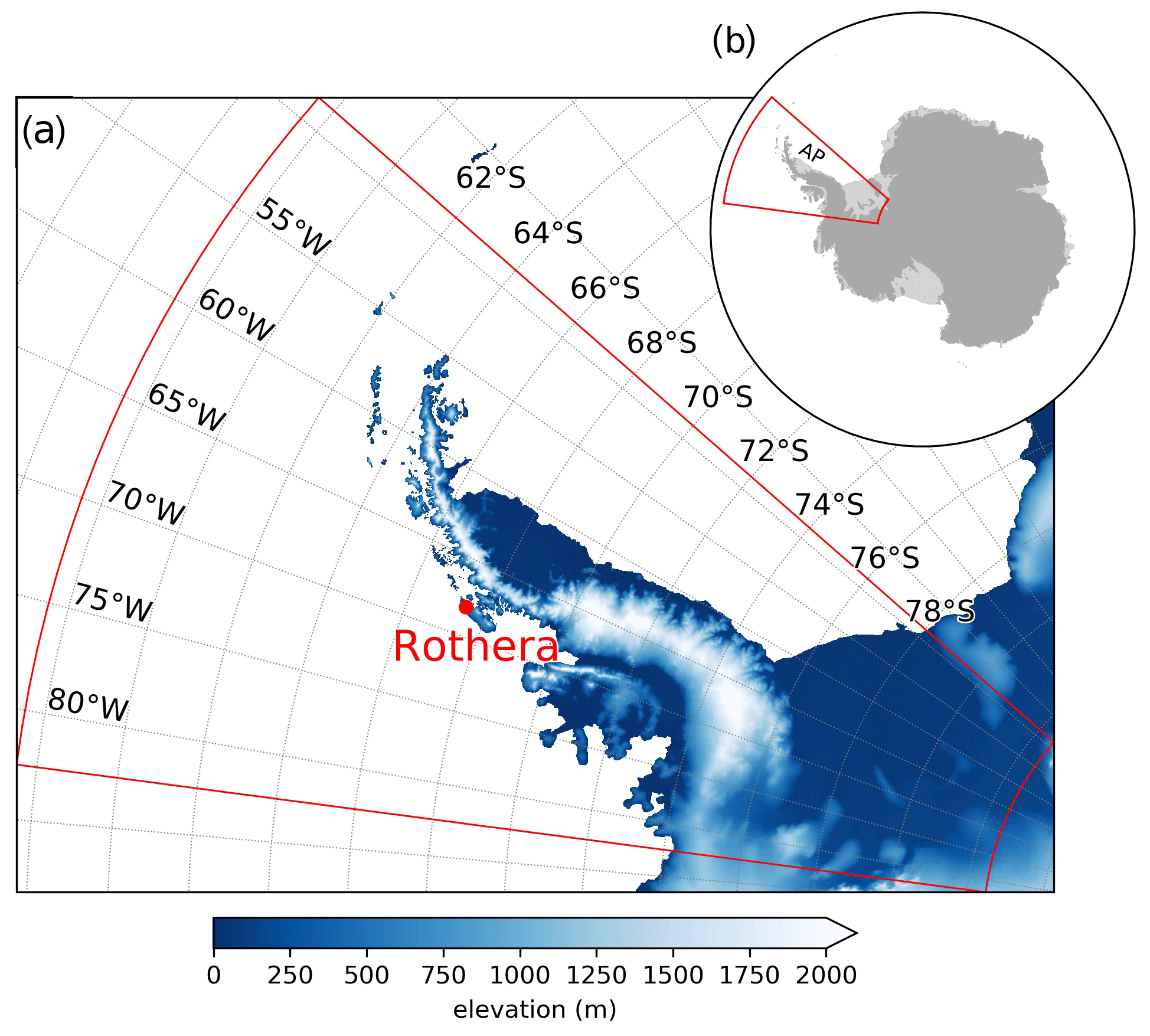
Figure 1Maps of the (a) Antarctic Peninsula region showing the box used to compute both the parameterised and AIRS results, as well as the location of Rothera Research Station where the radiosondes are launched and the elevation of the orography, and (b) Antarctica, with the locations of both the box and the Antarctic Peninsula (AP) indicated. Note that orography dataset used in panel (a) is Bedmap2 (Fretwell et al., 2013).
2.3 Methodology
To verify the parameterised mountain-wave-induced stratospheric cooling phase, 6-hourly values of for May–June–July–August–September–October over the Antarctic Peninsula from the perturbation run were compared against brightness temperature fluctuations measured by AIRS and temperature fluctuations measured by the radiosonde soundings. The brightness temperature fluctuations measured by AIRS are determined by removing a fourth-order polynomial function, representing the background atmosphere, from the original brightness temperatures (see Orr et al., 2015). To facilitate a comparison with the AIRS-observed minimum brightness temperature fluctuations() over the Antarctic Peninsula, the values of are converted into brightness temperature () by computing a weighted-sum of over all vertical model levels from 15 to 45 km, i.e. by summing the value of multiplied by the associated normalised weighting function for the 666.5 cm−1 radiance channel of AIRS over the range of vertical levels. Figure 1 shows the regions over the Antarctic Peninsula that were used to compute and . Note that the weighting function of the 666.5 cm−1 radiance channel is largely insensitive to atmospheric temperatures at altitudes both above 45 km and below 15 km. For the radiosonde-based measurements, we focus on the temperature perturbations observed at an altitude of between 20.2 and 20.6 km above sea level (chosen because this range is both in the lower stratosphere and includes the vertical level of the UM-UKCA model at a height of 20.4 km for comparison), which are computed by removing a third-order polynomial function representing the background atmosphere from the original profile (see Moffat-Griffin et al., 2011). The distributions for the parameterised fluctuations are compared with those for the measurements and the probability density functions generated using a kernel density estimation.
We use output from the two simulations to examine the temperature distribution T−TNAT and T−Tice, where T is equal to either (as used by the perturbation run) or TUM−UKCA (as used by the control run), and TNAT and Tice are the actual threshold temperatures for the existence of PSCs composed of NAT and water ice particles, respectively. The values computed for TNAT and Tice are sensitive to the temperature, pressure, HNO3 and water vapour mixing ratio (Hansen and Mauersberger, 1988; Marti and Mauersberger, 1993), which are taken from either the perturbation or control runs. We also compute for each run the FP of PSCs at an altitude of around 20.4 km, using a metric which depends on both the size of the temperature difference below either TNAT or Tice and the area of the region. For example, the FP for PSCs composed of NAT particles would be defined as
where i is an integer, N is the total number of model grid boxes within the region defined in Fig. 1, and Ai is the spatial area of the model grid box. An analogous equation exists for the FP for PSCs composed of water ice. Note that as the latitude–longitude grid used by the UM-UKCA model has non-uniform spacing and grid box area (due to varying longitude), the results from (1) are also scaled by the cosine of latitude. Note also that again the results are computed for the box situated over the Antarctic Peninsula shown in Fig. 1.
To identify the role of atmospheric conditions on controlling the parameterised stratospheric temperature fluctuations, the sensitivity of the amplitude of the cooling-phase to the vertical wind shear α is examined, with
where z1=0.85 km, z2=21.0 km and here U is the zonal wind velocity (applicable because the large-scale wind regime over the region containing the Antarctic Peninsula is predominately zonal; Thompson and Wallace, 2000). Note that this approach would not represent the impact of more local variations in α that also influence vertical propagation (Kruse et al., 2016). Additionally, the sensitivity of to directional shear was also investigated by examining its relationship to a change in the direction of the wind with height, between z2 and z1. These results are again computed for the box shown in Fig. 1.
Finally, we investigated the local impact of the scheme on ozone chemistry by examining changes in both the surface area density of PSCs composed of NAT particles and the ClONO2 (chlorine nitrate) + HCl (hydrochloric acid) reaction. This heterogeneous reaction is crucial as in their gas phase HCl and ClONO2 are very unreactive, and so any chlorine they contain is unable to destroy ozone (Solomon, 1999). However, in the presence of a PSC surface (either solid or liquid) they can react with each other to produce Cl2 (chorine gas), as well as the removal of nitric acid (HNO3) from the atmosphere, resulting in the denitrification of the stratosphere, an effect which allows Cl2 to build up during wintertime. In the spring, the presence of solar ultraviolet radiation splits Cl2 into two chlorine atoms (so-called chlorine activation), which plays an important role in stratospheric ozone depletion (Solomon, 1999). Note that these results are calculated over the region 76–64∘ S and 75–55∘ W, which includes the Antarctic Peninsula but is not the box depicted in Fig. 1. Furthermore, to look at the non-local impacts we examined changes to ozone over the high-latitude Southern Hemisphere, as well as temperature and pressure changes in the lower stratosphere, i.e. the polar vortex. Keeble et al. (2014) previously showed that in the version of UM-UKCA used here polar ozone depletion can have significant impacts on the polar vortex.
3.1 Comparison with observations
Figure 2 compares the probability distributions of and over the Antarctic Peninsula from May to October, showing that both distributions peak at similar values (around −0.5 K for and −1 K for ) but differ in terms of their shape, with restricted to a relatively narrow range and a high peak compared to a broader range and lower peak for . However, the agreement between the two distributions improves over the lower and large cooling part of the tail, with both showing a lower bound of around −6 K, which is perhaps the region of the distribution that is critical for decreasing temperatures below the threshold for PSC formation (particularly during early winter and early spring). Note that possible reasons for the discrepancies between the two distributions could be that (a) the parameterised results only represent mountain-wave-induced disturbances, while AIRS results include contributions from both orographic and non-orographic source regions, and (b) the (vertical-only propagation) parameterisation scheme does not represent the horizontal propagation of waves (Preusse et al., 2002; Sato et al., 2012), which could be potentially important here and result in a horizontal shift of mountain wave activity away from the source region. There is a much better agreement between the distributions of and over Rothera Research Station at an altitude of around 20.4 km (Fig. 3), with both distributions showing a relatively narrow range which peaks at a value of around −0.5 K, and the lower–cooling part of the tail extending to around −8 K. Note that the radiosonde results may also include contributions from non-orographic sources, such as from waves generated by the edge of the polar stratospheric vortex (Moffat-Griffin et al., 2011). Both Figs. 2 and 3 suggest that Antarctic Peninsula mountain waves with relatively large amplitudes of 5–10 K are uncommon (although it is noted that Eckermann et al. (2009) observed waves in this region with an amplitude of around 10 K for a particular case study).
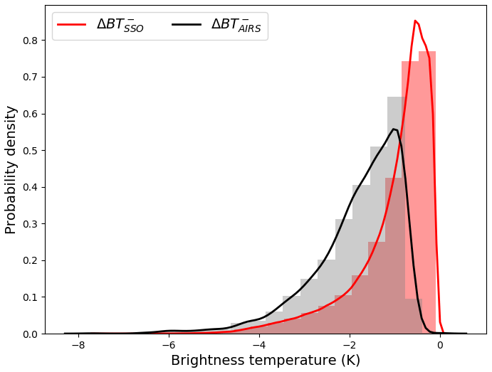
Figure 2Comparison of the probability distribution of brightness temperature perturbations (K) due to mountain-wave-induced stratospheric cooling over the Antarctic Peninsula between the parameterisation scheme (red line) and the AIRS observations (black line) for May to October. The AIRS values are from the 666.5 cm−1 radiance channel, for a 16-year period from 2002 to 2017 (and includes some contribution from non-orographic wave sources). The parameterised values are the weighted sum of from the perturbation run over all vertical model levels from 15 to 45 km (using the AIRS kernel function for the 666.5 cm−1 radiance channel), which is required to convert to . Note that a minimum threshold of BT < −0.1 K is used to reduce the inclusion of noise and spurious events. Both the parameterised and AIRS results are computed within the box indicated in Fig. 1.
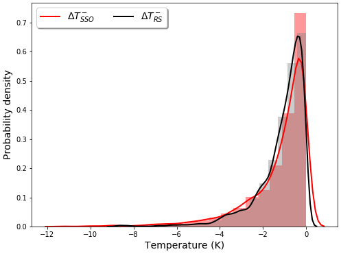
Figure 3Comparison of the probability distribution of the temperature perturbations (K) due to mountain-wave-induced cooling over Rothera Research Station on the Antarctic Peninsula between the parameterisation scheme (red line) and the radiosonde observations (black line) for May to October at an altitude of around 20.4 km. The radiosondes are launched around two to four times a week from Rothera for a 14-year period from 2002 to 2015 (see Fig. 1 for location) and compared against parameterised values from the perturbation run, which are taken from the grid box that contains this location. Note that a minimum threshold of T < −0.1 K is used to reduce the inclusion of noise and spurious events.
Figure 4 shows maps detailing the location and frequency of instances when K and K, i.e. the regions that contribute the most to the probability distributions shown in Fig. 2. The peak source region of the parameterised values is over the midsection and highest region (see Fig. 1) of the Antarctic Peninsula, i.e. centred over Alexander Island and Graham Land, which are regions of maximum σ (standard deviation of the SSO) in the UM-UKCA model (not shown). Note that here there are some contributions/waves from regions over the sea, which is due to the smoothness of the UM-UKCA mean orography (due to its relatively coarse resolution), which results in non-zero values of mean orography and associated SSO values over sea points around the coastline. By contrast, the AIRS-observed values show the peak source region to be more over the northern section of the Antarctic Peninsula. Note that the AIRS-observed values also show some contributions from over the sea surrounding the peninsula, which as discussed earlier is a possible reason for some of the disagreement between the distributions of parameterised and AIRS-observed cooling phase in Fig. 2.

Figure 4Map of the normalised number of instances that mountain-wave-induced cooling occurs over the Antarctic Peninsula in the (a) parameterised and (b) AIRS observations for May to October. Both the parameterised and AIRS results are based on the same information used to produce the probability distributions in Fig. 2. Note that the AIRS results also include some contribution from non-orographic wave sources. Note also that the maximum number is used to rescale and normalise the values from 0 to 1.
3.2 Impact on minimum temperatures and formation potential of PSCs
The distributions of temperature difference T−TNAT and T−Tice from the perturbation and control runs are shown in Fig. 5 for the combined months of May to October, and reveal that the addition of to the explicitly resolved synoptic-scale temperature TUM−UKCA (i.e. ) in the perturbation run is particularly important for temperatures to drop below Tice, as without this the temperature rarely falls below the ice frost point temperature by more than a few degrees kelvin. For PSCs composed of water ice particles, the addition of to the synoptic-scale temperature in the perturbation run extends the lower bound of the distribution from around or −3 K to K. For PSCs composed of NAT particles it is extended from around K to K. Figure 6 is analogous to Fig. 5, but comparing the distributions of the temperature differences T−TNAT and T−Tice for the individual months of May to October for the perturbation and control runs, indicating that the additional cooling in the perturbation run is vital if T is to drop below Tice during the months of May, June, September and October – as during these months in the control run alone is too warm, i.e. late austral autumn–early austral winter, as well as early austral spring (consistent with the findings of McDonald et al., 2009). Note however that during July and August the cold side of the tail extends to T−Tice < 0 K in the control run using . For PSCs composed of NAT particles the impact of the parameterisation in the perturbation run is particularly important for October (and to a lesser degree September), as this is the only month that the additional cooling is required for T to drop below TNAT, increasing the likelihood of PSC formation in early austral spring. However, it should be noted that the impact on PSC formation is also dependent on the local mixing ratios of HNO3 and H2O, which in part are affected by PSC formation and sedimentation earlier in the winter. We explore the impacts of the parameterisation on PSC surface area density in Sect. 3.4.
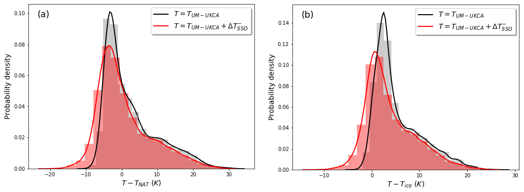
Figure 5Comparison of the probability distributions of the temperature differences (K) for (a) T−TNAT and (b) T−Tice over the Antarctic Peninsula at an altitude of 20.4 km for the combined months of May to October for the perturbation run (red line) and the control run (black line), i.e. for T equal to either (perturbation run with the parameterisation scheme on) or TUM−UKCA (control run with the parameterisation scheme off). Note that the results are computed within the box indicated in Fig. 1.

Figure 6As Fig. 5, but for the individual months from May (top row) to October (bottom row), with the panels on the left-hand side showing results for PSCs composed of NAT particles (T−TNAT) and on the right-hand side for PSCs composed of water ice particles (T−Tice) at an altitude of 20.4 km. Results are shown for the perturbation run (red line) and the control run (black line), i.e. for T equal to either (perturbation run with the parameterisation scheme on) or TUM−UKCA (control run with the parameterisation scheme off). The vertical dashed line denotes either or . Note that the results are computed within the box indicated in Fig. 1.
Using (1), Fig. 7 shows the FP for PSCs composed of both water ice and NAT particles at an altitude of 20.4 km for the individual months from May to October from both the perturbation and control runs. This shows that the FP of PSCs composed of NAT particles is around 2 orders of magnitude larger than that for PSCs composed of water ice particles due to them having a higher threshold temperature for formation (i.e. roughly around 195 K for TNAT and 188 K for Tice at this altitude). Thus it is much more likely that the temperature falls below the threshold temperature (cf. Figs. 5 and 6). The results show FP values for NAT particles peaking at around K km2 in June and July, but with little sensitivity in any of the months to the inclusion of the additional cooling in the perturbation run. However, consistent with Fig. 6 is that the FP of PSCs composed of water ice particles is highly sensitive to the inclusion of the additional cooling in the perturbation run, with FP values around 4–5 times larger in July and August if the additional cooling is included compared to it being neglected in the control run, as well as significant increases also occurring during June and September, which otherwise show a negligible FP for the control run. For PSC composed of NAT particles, the FP values obtained from the perturbation and control run are much more similar (cf. Figs. 5 and 6), although the inclusion of the added cooling in the perturbation run does still result in increases. To further understand this, Fig. 8 shows maps of the difference in FP between the perturbed and control runs for the two types of PSCs examined, revealing that the differences evident in Fig. 7 (i.e. due to the addition of to the synoptic-scale temperature) are dominated by the contribution from mountain waves originating from the high-altitude base of the Antarctic Peninsula (which Hoffmann et al., 2013, showed was a hotspot of mountain wave activity).
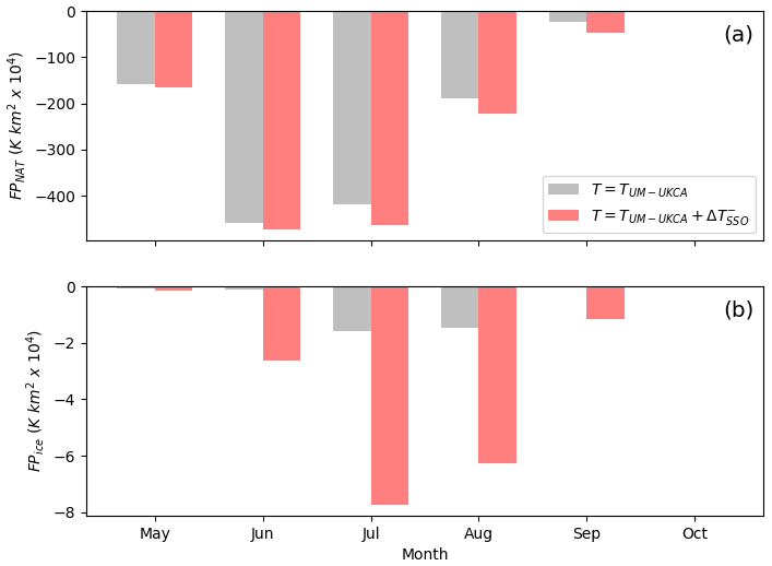
Figure 7Histograms showing the monthly mean formation potential (× 104 K km2; see (1) for definition) for PSCs made from (a) NAT and (b) ice particles during each individual month from May to October at an altitude of 20.4 km for the perturbation run (red) and the control run (grey), i.e. for T equal to either (perturbation run with the parameterisation scheme on) or TUM−UKCA (control run with the parameterisation scheme off). Note that the results are computed within the box indicated in Fig. 1.
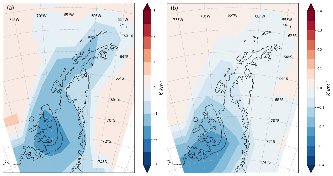
Figure 8Maps of the differences in mean monthly FP (K km2) between the perturbation run and the control run for the combined months of May to October over the Antarctic Peninsula at an altitude of 20.4 km for PSCs composed of (a) NAT and (b) ice particles, i.e. the difference between using T equal to either (perturbation run with the parameterisation scheme on) or TUM−UKCA (control run with the parameterisation scheme off).
3.3 Conditions required for large localised negative temperature anomalies
Using (2), Fig. 9 compares the range of vertical wind shear α that was associated with the top 10 % (i.e. most cold) and bottom 10 % (i.e. least cold) of the distribution of the cooling phase at an altitude of 20.4 km. This shows that the largest negative cooling phases are associated with larger (positive) values of α, which is consistent with the understanding that waves with long vertical wavelengths in the stratosphere generate large temperature fluctuations and are associated with conditions where wind speed increases with height, i.e. causing wave refraction towards longer vertical wavelengths (Wu and Eckermann, 2008; Bramberger et al., 2017). Hoffmann et al. (2017) also showed that such conditions were conducive for the propagation of gravity waves into the lower stratosphere with long vertical wavelengths, which AIRS can best identify. Note that the top 10 % and bottom 10 % of the distribution were comparatively insensitive to the change in wind direction with height (not shown), which perhaps reflects that the wind regime is predominately unidirectional with height, i.e. a similar structure at many height levels in both the troposphere and lower stratosphere, consistent with an equivalent barotropic structure (Thompson and Wallace, 2000).

Figure 9Box-and-whisker plot showing the range of the vertical wind shear α (see (2) for definition) for the (a) top 10 % and (b) bottom 10 % of the probability distribution of the parameterised cooling phase over the Antarctic Peninsula from the perturbed run for May to October at an altitude of 20.4 km, i.e. the most cold (top 10 %) and least cold (bottom 10 %) of the cooling-phase events. Note that the results are computed within the box indicated in Fig. 1.
3.4 Impact on chlorine activation and PSCs over the Antarctic Peninsula
The impact of the additional cooling in the perturbation run on PSCs composed of NAT particles and chlorine activation is shown in Fig. 10. In the control run, the maximum surface area density of PSCs composed of NAT particles is modelled in June at an altitude of around 20 km, and extending from around 10 to 30 km. Between June and September, the surface area of the NAT particles decreases due to both rising (synoptic-scale) temperatures and the effects of denitrification and dehydration of the polar vortex by PSC sedimentation (Fahey et al., 1990; Teitelbaum et al., 2001). The result is that by August and September, little PSC surface area remains for chlorine activation. However, in the perturbation run, the surface area density of the NAT particles is increased at higher altitudes throughout the winter and early spring and reduced at lower altitudes. Importantly for chlorine activation in the late winter and spring (August and September), surface area density is increased by up to 20 %. Also shown in Fig. 10 is the flux through the ClONO2+ HCl heterogeneous reaction, a key reaction for the activation of chlorine from the major chlorine reservoir species. Surface area density changes of the NAT particles have only a modest impact on chlorine activation throughout the winter, but the small increases in surface area density in the late winter and early spring in the perturbation experiment result in large increases in chlorine activation throughout August and September, and thus enhancing ozone depletion (Solomon, 1999).
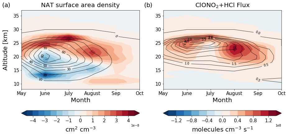
Figure 10Altitude versus time plots of the differences in (a) NAT PSC surface area density ( cm2 cm−3; shading) and (b) the flux through the ClONO2+ HCl reaction (× 108 molecules cm−3 s−1; shading) between the perturbed run and the control run, averaged over the Antarctica Peninsula (over the region 76–64∘ S and 75–55∘ W), i.e. the difference between using T equal to either (perturbation run with the parameterisation scheme on) or TUM−UKCA (control run with the parameterisation scheme off). Also shown in each panel are the respective values from the control simulation using a value of T equal to TUM−UKCA (contours).
3.5 Impact on mean total column ozone, temperature and pressure over the high-latitude Southern Hemisphere
Figure 11 shows the impact of the additional cooling in the perturbation run on October monthly mean total column ozone. While Fig. 10 highlights the local impacts of the parameterisation scheme on PSC formation and chlorine activation, it can be seen from Fig. 11 that the impacts of the parameterisation scheme extend far beyond the region of the Antarctic Peninsula. This is unsurprising, as not only is the Antarctic Peninsula responsible for differences both upstream and downstream of the region, but other hotspots of mountain wave activity exist over Antarctica that can also play a role in PSC formation, such as the Transantarctic Mountains (e.g. Noel et al., 2009; Hoffmann et al., 2013, 2017; Alexander et al., 2017), which would also be sources of cooling via the parameterisation scheme. While perhaps it would be expected that October monthly mean total column ozone would be reduced above and downwind from the Antarctic Peninsula when the additional cooling is included in the perturbation run, there is little change to column ozone values here. Instead, total column ozone is reduced between 30 and 130∘ E and increased between 120 and 180∘ W. This is indicative of a shift of the polar vortex away from the Pacific sector of the Southern Ocean and towards the Indian Ocean sector. This result is supported by the 25 km pressure and temperature differences between the two simulations, which both indicate a change in the position of the polar vortex (Fig. 11).
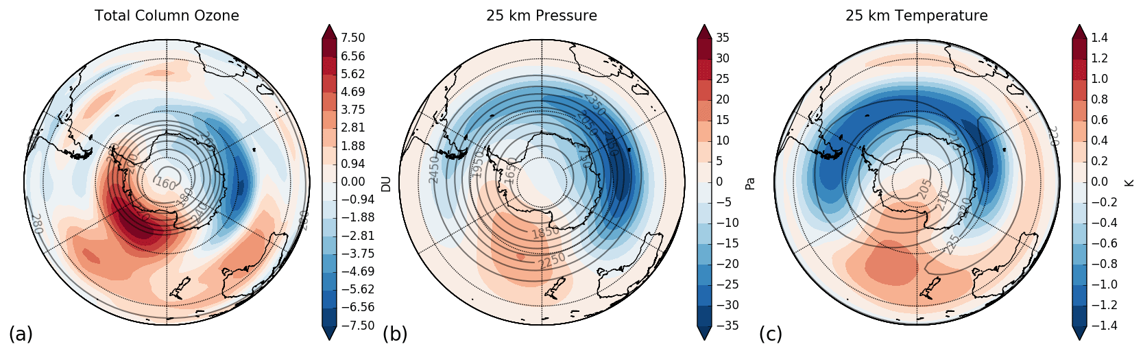
Figure 11Maps of the average differences in October monthly mean total column ozone (a) (units of Dobson units), 25 km pressure (b) (units of pascals) and 25 km temperature (c) (units of kelvin) between the perturbed run and the control run, i.e. the difference between using T equal to either (perturbation run with the parameterisation scheme on) or TUM−UKCA (control run with the parameterisation scheme off). Also shown in each panel are the respective values from the control simulation using a value of T equal to TUM−UKCA (contours).
Mountain-wave-induced PSC formation, which is a significant influence on ozone chemistry, is missing from current coarse-resolution global chemistry–climate models because the small-scale temperature fluctuations associated with mountain waves are neither resolved nor parameterised – limiting our ability to make accurate predictions of stratospheric ozone. This study examines in detail an attempt to make global chemistry–climate models more physically based and comprehensive by including a novel parameterisation of mountain-wave-induced temperature fluctuations inserted into a 30-year run of the global chemistry–climate configuration of the UM-UKCA global chemistry–climate model.
The study firstly examined the detailed representation of episodic and localised wintertime stratospheric cooling phases over the Antarctic Peninsula, secondly the subsequent impact of the cooling phases on local chlorine activation and PSC formation, and thirdly the impacts of the scheme over the entire high-latitude Southern Hemisphere (i.e. the inclusion of mountain-wave-induced cooling phases from many other orographic hotspots and not just the Antarctic Peninsula) on ozone and the stratospheric polar vortex. The main findings were as follows.
-
The probability distribution of the parameterised cooling phases are in reasonable agreement with values derived from long-term AIRS brightness temperature measurements (with a possible reason for the discrepancy being that AIRS also includes contributions from non-orographic source regions) and in excellent agreement with values derived from long-term radiosonde temperature soundings from Rothera Research Station situated on the Antarctic Peninsula.
-
In both cases the agreement with the AIRS and radiosonde values was particularly good for the lower–large cooling part of the tail of the distributions, with a lower bound of up to −6 K for and and up to −8 K for and , which is perhaps the region of the distribution that is critical for decreasing temperatures below the threshold for PSC formation (particularly during early winter and early spring).
-
The addition of to the resolved and synoptic-scale temperatures in the UM-UKCA model (i.e. ) results in a considerable increase in the number of instances when minimum temperatures fall below Tice during late austral autumn–early austral winter and early austral spring by extending the lower bound of the T−Tice distribution from around K to K; i.e. without the additional cooling phase the temperature in the model rarely falls below the ice frost point temperature by more than a degree kelvin or so during these periods.
-
The addition of extends the lower bound of the T−TNAT distribution from around K to K, although it is only during early austral spring that the additional cooling is required for T to drop below TNAT.
-
Values of the FP of PSCs composed of water ice particles are many times larger if the additional cooling is included. However, for PSCs consisting of NAT particles, although the additional cooling resulted in an increase in FP, it was small.
-
The addition of results in an increase in the surface area density of NAT particles throughout the winter and early spring, which is important for chlorine activation – evident in a large increase in the flux through the ClONO2+ HCl reaction throughout August and September.
-
Examination of the total column ozone during October shows that the addition of results in a reduction between 30 and 130∘ E and an increase between 120 and 180∘ W, indicative of a shift of the polar vortex away from the Pacific sector of the Southern Ocean and towards the Indian Ocean sector.
Note that Keeble et al. (2014) demonstrated that in the version of UM-UKCA used here that polar ozone depletion can have significant impacts on the polar vortex, affecting both the strength and latitude of the westerly polar jet, and this relationship has also been noted by other studies (e.g. McLandress et al., 2010; Son et al., 2010; Polvani et al., 2011). The study thus shows that both the local and non-local impacts of including the scheme are substantial and that inclusion of the scheme in a global chemistry–climate model is a step towards it becoming more consistent with our physically based understanding of the atmosphere. This, we suggest, is essential for understanding how models respond to changes to ozone-depleting substances and greenhouse gases and hence for improving predictions of ozone and the high-latitude Southern Hemisphere climate system.
Note also that next-generation models, such as the ICON-ART (ICOsahedral Nonhydrostatic model with Aerosols and Reactive Trace gases) global modelling system (Schröter et al., 2018), may be able to employ variable spatial resolution with local grid refinement where the resolution increases locally over mountainous regions so that the mountain-wave-induced temperature fluctuations are resolved explicitly, negating the need for their parameterisation.
As one of the main aims of global chemistry–climate models is the prediction of ozone, which to determine accurately requires a realistic treatment of PSCs, further work will focus on assessing the representation of PSCs in this state-of-the-art configuration of the UM-UKCA by comparing results in both hemispheres against a comprehensive climatology of PSC coverage based on MIPAS (Michelson Interferometer for Passive Atmospheric Sounding) observations (Spang et al., 2018). Moreover, although the UM-UKCA model (in common with many other global climate models) employs a rather simplistic PSC scheme which limits its ability to accurately predict ozone, the improved representation of PSC formation detailed in this study will also eventually be used to develop better projections of future polar ozone levels in response to climate change, such as narrowing uncertainties in the rate and timing of the closure of the Antarctic ozone hole (Eyring et al., 2013).
The AIRS measurements of brightness temperature perturbations used in this study can be downloaded from https://datapub.fz-juelich.de/slcs/airs/gravity_waves (re3data.org, 2020). The high-resolution radiosonde data from Rothera Research Station can be downloaded from https://catalogue.ceda.ac.uk/uuid/37f2bef57e28bcd780a5cbfe077f4bf8 (British Antarctic Survey, 2008). Please contact the lead author if you would like access to the UM-UKCA output.
AO, JSH and AD conceived and worked on the research project, with AD undertaking much of the analysis for this study during a 4-month internship at the British Antarctic Survey. JSH subsequently revised many of the plots included in the manuscript. AO implemented the parameterisation scheme into the UM-UKCA model and also ran the model simulations. AO also wrote the majority of the paper. Many of the ideas for the work were generated during a mini-workshop at the British Antarctic Survey, which was attended by all the authors. LH provided the AIRS-based observations and expertise on how they should be utilised. RS provided expert advice on the calculation of temperature thresholds for PSC formation. TMG provided the radiosonde data and advice on how it should be used. JK produced the plots investigating local PSC formation and heterogeneous chemistry, as well the non-local impacts of the scheme by examining changes to ozone as well as the position of the polar vortex. NLA provided expert advice on the setting up and running of the UM-UKCA simulations. Additionally, all authors contributed to the interpretation and writing of the paper.
The authors declare that they have no conflict of interest.
We thank the two anonymous reviewers who provided helpful comments on an earlier version of this paper. This work used the ARCHER UK National Supercomputing Service. We acknowledge the hard work of the Rothera field staff, who made the radiosonde measurements.
This work was undertaken as part of the Polar Science for Planet Earth Programme of the British Antarctic Survey and funded by the Natural Environment Research Council (NERC). James Keeble and Nathan Luke Abraham thank NERC through NCAS for financial support.
This paper was edited by Michael Pitts and reviewed by two anonymous referees.
AIRS/Aqua Observations of Gravity Waves, re3data.org – Registry of Research Data Repositories, http://doi.org/10.17616/R34J42, 2020.
Alexander, J. M. and Teitelbaum, H.: Observation and analysis of a large amplitude mountain wave event over the Antarctic Peninsula, J. Geophys. Res., 112, D21103, https://doi.org/10.1029/2006JD008368, 2007.
Alexander, S. P., Klekociuk, A. R., Pitts, M. C., McDonald, A. J., and Arevalo-Torres, A.: The effect of orographic gravity waves on Antarctic polar stratosphere cloud occurrence and composition, J. Geophys. Res., 116, D06109, https://doi.org/10.1029/2010JD015184, 2011.
Alexander, S. P., Klekociuk, A. R., McDonald, A. J., and Pitts, M. C.: Quantifying the role of orographic gravity waves on polar stratospheric cloud occurrence in the Antarctic and the Arctic, J. Geophys. Res., 118, 11493–11507, https://doi.org/10.1002/2013JD020122, 2013.
Alexander, S., Orr, A., Webster, S., and Murphy, D.: Observations and fine-scale model simulations of gravity waves over Davis, East Antarctica (69∘ S, 78∘ E), J. Geophys. Res., 122, 7355–7370, https://doi.org/10.1002/2017JD026615, 2017.
Alfred, J., Fromm, M., Bevilacqua, R., Nedoluha, G., Strawa, A., Poole, L., and Wickert, J.: Observations and analysis of polar stratospheric clouds detected by POAM III and SAGE III during the SOLVE II/VINTERSOL campaign in the 2002/2003 Northern Hemisphere winter, Atmos. Chem. Phys., 7, 2151–2163, https://doi.org/10.5194/acp-7-2151-2007, 2007.
Bacmeister, J. T., Schoeberl, M. R., Lait, L. R., Newman, P. A., and Gary, B.: ER-2 mountain wave encounter over Antarctica: Evidence for blocking, Geophys. Res. Lett., 17, 81–84, https://doi.org/10.1029/GL017i001p00081,1990.
Bramberger, M., Dörnbrack, A., Bossert, K., Ehard, B., Fritts, D. C., Kaifler, B., Mallaun, C., Orr, A., Pautet, P.-Dominique, Rapp, M., Taylor, M. J., Vosper, S., Williams, B. P., and Witschas, B.: Does strong tropospheric forcing cause large-amplitude mesospheric gravity waves? A DEEPWAVE case study, J. Geophys. Res., 122, 11422–11443, https://doi.org/10.1002/2017JD027371, 2017.
British Antarctic Survey: high resolution radiosonde data from Halley and Rothera stations, NCAS British Atmospheric Data Centre, 2020, http://catalogue.ceda.ac.uk/uuid/37f2bef57e28bcd780a5cbfe077f4bf8, 2008.
Campbell, J. R. and Sassen, K.: Polar stratospheric clouds at the South Pole from 5 years of continuous lidar data: Macrophysical, optical, and thermodynamic properties, J. Geophys. Res., 113, D20204, https://doi.org/10.1029/2007JD009680, 2008.
Carslaw, K., Wirth, M., Tsias, A., Luo, B. P., Dörnbrack, A., Leutbecher, M., Volkert, H., Renger, W., Bacmeister, J. T., Reimer, E., and Peter, Th.: Increased stratospheric ozone depletion due to mountain-induced atmospheric waves, Nature, 391, 675–678, https://doi.org/10.1038/35589, 1998.
Chiodo, G. and Polvani, L. M.: Reduced Southern Hemisphere circulation response to quadrupled CO2 due to stratospheric ozone feedback, Geophys. Res. Lett., 44, 465–474, https://doi.org/10.1002/2016GL071011, 2017.
Chipperfield, M. P.: Multiannual simulations with a 3D chemical transport model, J. Geophys. Res., 104, 1781–1805, https://doi.org/10.1029/98JD02597, 1999.
Dean, S. M., Flowerdew, J., Lawrence, B. N., and Eckermann, S. D.: Parameterisation of orographic cloud dynamics in a GCM, Clim. Dynam., 28, 581–597, https://doi.org/10.1007/s00382-006-0202-0, 2007.
Dörnbrack, A., Leutbecher, M., Kivi, R., and Kyrö, E.: Mountain wave-induced record low stratospheric temperatures above northern Scandinavia, Tellus, 51, 951–963, https://doi.org/10.1034/j.1600-0870.1999.00028.x, 1999.
Dörnbrack, A. and Leutbecher, M.: Relevance of mountain waves for the formation of polar stratospheric clouds over Scandinavia: A 20-year climatology, J. Geophys. Res., 106, 1583–1593, https://doi.org/10.1029/2000JD900250, 2001.
Dörnbrack, A., Birner, T., Fix, A., Flentje, H., Meister, A., Schmid, H., Browell, E. V., and Mahoney, M. J.: Evidence for inertia gravity waves forming in polar stratospheric clouds over Scandinavia, J. Geophys. Res., 107, 8287, https://doi.org/10.1029/2001JD000452, 2002.
Eckermann, S. D., Hoffmann, L., Höpfner, M., Wu, D. L., and Alexander, M. J.: Antarctic NAT PSC belt of June 2003: Observational validation of the mountain wave seeding hypothesis, Geophys. Res. Lett., 36, L02807, https://doi.org/10.1029/2008GL036629, 2009.
Eyring, V., Arblaster, J. M., Cionni, I., Sedlácek, J., Perlwitz, J., Young, P. J., Bekki, S., Bergmann, D., Cameron-Smith, P., Collins, W. J., Faluvegi, G., Gottschaldt, K.-D., Horowitz, L. W., Kinnison, D. E., Lamarque, J.-F., Marsh, D. R., Saint-Martin, D., Shindell, D. T., Sudo, K., Szopa, S., and Watanabe, S.: Long-term ozone changes and associated climate impacts in CMIP5 simulations, J. Geophys. Res., 118, 5029–5060, https://doi.org/10.1002/jgrd.50316, 2013.
Fahey, D. W., Kelly, K. K., Kawa, S. R., Tuck, A. F., Loewenstein, M., Chan, K. R., and Heidt, L. E.: Observations of denitrification and dehydration in the winter polar stratospheres, Nature, 344, 321–324, https://doi.org/10.1038/344321a0, 1990.
Farman, J., Gardiner, B., and Shanklin, J.: Large losses of total ozone in Antarctica reveal seasonal ClOx/NOx interaction, Nature, 315, 207–210, https://doi.org/10.1038/315207a0, 1985.
Fretwell, P., Pritchard, H. D., Vaughan, D. G., Bamber, J. L., Barrand, N. E., Bell, R., Bianchi, C., Bingham, R. G., Blankenship, D. D., Casassa, G., Catania, G., Callens, D., Conway, H., Cook, A. J., Corr, H. F. J., Damaske, D., Damm, V., Ferraccioli, F., Forsberg, R., Fujita, S., Gim, Y., Gogineni, P., Griggs, J. A., Hindmarsh, R. C. A., Holmlund, P., Holt, J. W., Jacobel, R. W., Jenkins, A., Jokat, W., Jordan, T., King, E. C., Kohler, J., Krabill, W., Riger-Kusk, M., Langley, K. A., Leitchenkov, G., Leuschen, C., Luyendyk, B. P., Matsuoka, K., Mouginot, J., Nitsche, F. O., Nogi, Y., Nost, O. A., Popov, S. V., Rignot, E., Rippin, D. M., Rivera, A., Roberts, J., Ross, N., Siegert, M. J., Smith, A. M., Steinhage, D., Studinger, M., Sun, B., Tinto, B. K., Welch, B. C., Wilson, D., Young, D. A., Xiangbin, C., and Zirizzotti, A.: Bedmap2: improved ice bed, surface and thickness datasets for Antarctica, The Cryosphere, 7, 375–393, https://doi.org/10.5194/tc-7-375-2013, 2013.
Goff, J. A.: Saturation pressure of water on the new Kelvin temperature scale, Trans. Am. Soc. Heating and Vent. Eng., 63, 347–354, 1957.
Hanson, D. and Mauersberger, K.: Laboratory studies of the nitric acid trihydrate: implications for the south polar stratosphere, Geophys. Res. Lett., 15, 855–858, https://doi.org/10.1029/GL015i008p00855, 1988.
Hersbach, H., Bell, B., Berrisford, P., Hirahara, S., Horányi, A., Joaquín, M.-S., Nicolas, J., Peubey, C., Radu, R., Schepers, D., Simmons, A., Soci, C., Abdalla, S., Abellan, X., Balsamo, G., Bechtold, P., Biavati, G., Bidlot, J., Bonavita, M., De Chiara , G., Dahlgren, P., Dee, D., Diamantakis, M., Dragani, R., Flemming, J., Forbes, R., Fuentes, M., Geer, A., Haimberger, L., Healy, S., Hogan, R., Hólm, E., Janisková, M., Keeley, S., Laloyaux, P., Lopez, P., Lupu, C., Radnoti, G., de Rosnay, P., Rozum, I., Vamborg, F., Villaume, S., and Thépaut, J.-N.: The ERA5 global reanalysis, Q. J. Roy. Meteor. Soc., 146, 1999–2049, https://doi.org/10.1002/qj.3803, 2020.
Hewitt, H. T., Copsey, D., Culverwell, I. D., Harris, C. M., Hill, R. S. R., Keen, A. B., McLaren, A. J., and Hunke, E. C.: Design and implementation of the infrastructure of HadGEM3: the next-generation Met Office climate modelling system, Geosci. Model Dev., 4, 223–253, https://doi.org/10.5194/gmd-4-223-2011, 2011.
Hoffmann, L., Xue, X., and Alexander, M. J.: A global view of stratospheric gravity wave hotspots located with Atmospheric Infrared Sounder observations, J. Geophys. Res., 118, 416–434, https://doi.org/10.1029/2012JD018658, 2013.
Hoffmann, L., Grimsdell, A. W., and Alexander, M. J.: Stratospheric gravity waves at Southern Hemisphere orographic hotspots: 2003–2014 AIRS/Aqua observations, Atmos. Chem. Phys., 16, 9381–9397, https://doi.org/10.5194/acp-16-9381-2016, 2016.
Hoffmann, L., Spang, R., Orr, A., Alexander, M. J., Holt, L. A., and Stein, O.: A decadal satellite record of gravity wave activity in the lower stratosphere to study polar stratospheric cloud formation, Atmos. Chem. Phys., 17, 2901–2920, https://doi.org/10.5194/acp-17-2901-2017, 2017.
Iglesias-Suarez, F., Young, P. J., and Wild, O.: Stratospheric ozone change and related climate impacts over 1850–2100 as modelled by the ACCMIP ensemble, Atmos. Chem. Phys., 16, 343–363, https://doi.org/10.5194/acp-16-343-2016, 2016.
Keeble, J., Braesicke, P., Abraham, N. L., Roscoe, H. K., and Pyle, J. A.: The impact of polar stratospheric ozone loss on Southern Hemisphere stratospheric circulation and climate, Atmos. Chem. Phys., 14, 13705–13717, https://doi.org/10.5194/acp-14-13705-2014, 2014.
Kruse, C. G., Smith, R. B., and Eckermann, S. D.: The midlatitude lower-stratospheric mountain wave “valve layer”, J. Atmos. Sci., 73, 5081–5100, https://doi.org/10.1175/JAS-D-16-0173.1, 2016.
Marti, J. and Mauersberger, K.: A survey and new measurements of ice vapour pressure at temperatures between 170 and 250 K, Geophys. Res. Lett., 20, 363–366, https://doi.org/10.1029/93GL00105, 1993.
McDonald, A. J., George, S. E., and Woollands, R. M.: Can gravity waves significantly impact PSC occurrence in the Antarctic?, Atmos. Chem. Phys., 9, 8825–8840, https://doi.org/10.5194/acp-9-8825-2009, 2009.
McLandress, C., Jonsson, A. I., Plummer, D. A., Reader, M. C., Scinocca, J. F., and Shepherd, T. G.: Separating the dynamical effects of climate change and ozone depletion, Part I: Southern Hemisphere stratosphere, J. Climate, 23, 5002–5020, https://doi.org/10.1175/2010JCLI3586.1, 2010.
Moffat-Griffin, T., Hibbins, R. E., Jarvis, M. J., and Colwell, S. R.: Seasonal variations of gravity wave activity in the lower stratosphere over an Antarctic Peninsula station, J. Geophys. Res., 116, D14111, https://doi.org/10.1029/2010JD015349, 2011.
Morgenstern, O., Braesicke, P., O'Connor, F. M., Bushell, A. C., Johnson, C. E., Osprey, S. M., and Pyle, J. A.: Evaluation of the new UKCA climate-composition model – Part 1: The stratosphere, Geosci. Model Dev., 2, 43–57, https://doi.org/10.5194/gmd-2-43-2009, 2009.
Noel, V., Hertzog, A., and Chepfer, H.: CALIPSO observations of wave-induced PSCs with near-unity optical depth over Antarctica in 2006–2007, J. Geophys. Res., 114, D05202, https://doi.org/10.1029/2008JD010604, 2009.
Orr, A., Marshall, G., Hunt, J. C. R., Sommeria, J., Wang, C., van Lipzig, N., Cresswell, D., and King, J. C.: Characteristics of airflow over the Antarctic Peninsula and its response to recent strengthening of westerly circumpolar winds, J. Atmos. Sci., 65, 1396–1413, https://doi.org/10.1175/2007JAS2498.1, 2008.
Orr, A., Bracegirdle, T. J., Hoskings, J. S., Jung, T., Haigh, J. D., Phillips, T., and Feng, W.: Possible dynamical mechanisms for Southern Hemisphere climate change due to the ozone hole, J. Atmos. Sci., 69, 2917–2932, https://doi.org/10.1175/JAS-D-11-0210.1, 2012.
Orr, A., Hosking, J. S., Hoffmann, L., Keeble, J., Dean, S. M., Roscoe, H. K., Abraham, N. L., Vosper, S., and Braesicke, P.: Inclusion of mountain-wave-induced cooling for the formation of PSCs over the Antarctic Peninsula in a chemistry–climate model, Atmos. Chem. Phys., 15, 1071–1086, https://doi.org/10.5194/acp-15-1071-2015, 2015.
Pawson, S., Naujokat, B., and Labitzke, K.: On the polar stratospheric cloud formation potential of the northern stratosphere, J. Geophys. Res., 100, 23215–23225, https://doi.org/10.1029/95JD01918, 1995.
Plougonven, R., Hertzog, A., and Teitelbaum, H.: Observations and simulations of large-amplitude mountain wave breaking over the Antarctic Peninsula, J. Geophys. Res., 113, D16113, https://doi.org/10.1029/2007JD009739, 2008.
Plougonven, R., Hertzog, A., and Guez, L.: Gravity waves over Antarctica and the Southern Ocean: consistent momentum fluxes in mesoscale simulations and stratospheric balloon observations, Q. J. Roy. Meteor. Soc., 139, 101–118, https://doi.org/10.1002/qj.1965, 2012.
Polvani, L. M., Waugh, D. W., Correa, G. J. P., and Son, S.-W.: Stratospheric ozone depletion: The main driver of twentieth-century atmospheric circulation changes in the Southern Hemisphere, J. Climate, 24, 795–812, https://doi.org/10.1175/2010JCLI3772.1, 2011.
Pope, J. O., Orr, A., Marshall, G. J., and Abraham, N. L.: Non‐additive response of the high‐latitude Southern Hemisphere climate to aerosol forcing in a climate model with interactive chemistry. Atmos Sci Lett. e1004, https://doi.org/10.1002/asl.1004, 2020.
Preusse, P., Dörnbrack, A., Eckermann, S. D., Riese, M., Schaeler, B., Bacmeister, J. T., Broutman, D., and Grossmann, K. U.: Space‐based measurements of stratospheric mountain waves by CRISTA 1, sensitivity, analysis method, and a case study, J. Geophys. Res., 107, 8178, https://doi.org/10.1029/2001JD000699, 2002.
Previdi, M. and Polvani, L. M.: Climate system response to stratospheric ozone depletion and recovery, Q. J. Roy. Meteor. Soc., 140, 2401–2419, https://doi.org/10.1002/qj.2330, 2014.
Sato, K., Tateno, S., Watanabe, S., and Kawatani, Y.: Gravity wave characteristics in the Southern Hemisphere revealed by a high-resolution middle-atmosphere general circulation model, J. Atmos. Sci., 69, 1378–1396, https://doi.org/10.1175/JAS-D-11-0101.1, 2012.
Schröter, J., Rieger, D., Stassen, C., Vogel, H., Weimer, M., Werchner, S., Förstner, J., Prill, F., Reinert, D., Zängl, G., Giorgetta, M., Ruhnke, R., Vogel, B., and Braesicke, P.: ICON-ART 2.1: a flexible tracer framework and its application for composition studies in numerical weather forecasting and climate simulations, Geosci. Model Dev., 11, 4043–4068, https://doi.org/10.5194/gmd-11-4043-2018, 2018.
Solomon, S.: Stratospheric ozone depletion: A review of concepts and history, Rev. Geophys., 37, 275–316, https://doi.org/10.1029/1999RG900008, 1999.
Solomon, S., Garcia, R. R., Rowland, F. S., and Wuebbles, D. J.: On the depletion of Antarctic ozone, Nature, 321, 755–758, 1986.
Son, S.-W., Gerber, E. P., Perlwitz, J., Polvani, L. M., Gillett, N. P., Seo, K.-H., Eyring, V., Shepherd, T. G., Waugh, D., Akiyoshi, H., Austin, J., Baumgaertner, A., Bekki, S., Braesicke, P., Bruhl, C., Butchart, N., Chipperfield, M. P., Cugnet, D., Dameris, M., Dhomse, S., Frith, S., Garny, H., Garcia, R., Hardiman, S, C., Jockel, P., Lamarque, J. F., Mancini, E., Marchand, M., Michou, M., Nakamura, T., Morgenstern, O., Pitari, G., Plummer, D. A., Pyle, J., Rozanov, E., Scinocca, J. F., Shibata, K., Smale, D., Teyssedre, H., Tian, W., and Yamashita, Y.: Impact of stratospheric ozone on Southern Hemisphere circulation change: a multimodel assessment, J. Geophys. Res., 115, D00M07, https://doi.org/10.1029/2010JD014271, 2010.
Spang, R., Hoffmann, L., Müller, R., Grooß, J.-U., Tritscher, I., Höpfner, M., Pitts, M., Orr, A., and Riese, M.: A climatology of polar stratospheric cloud composition between 2002 and 2012 based on MIPAS/Envisat observations, Atmos. Chem. Phys., 18, 5089–5113, https://doi.org/10.5194/acp-18-5089-2018, 2018.
Teitelbaum, H., Moustaoui, M., and Fromm, M.: Exploring polar stratospheric cloud and ozone minihole formation: The primary importance of synoptic-scale flow perturbations, J. Geophys. Res., 106, 28173–28188, https://doi.org/10.1029/2000JD000065, 2001.
Thompson, D. W. J. and Solomon, S.: Interpretation of recent southern hemisphere climate change, Science, 296, 895–899, https://doi.org/10.1126/science.1069270, 2002.
Thompson, D. W. J. and Wallace, J. M.: Annular modes in the extratropical circulation, Part I: Month-to-month variability, J. Climate, 13, 1000–1016, https://doi.org/10.1175/1520-0442(2000)013<1000:AMITEC>2.0.CO;2, 2000.
Wu, D. L. and Eckermann, S. D.: Global gravity wave variances from Aura MLS: Characteristics and interpretation, J. Atmos. Sci., 65, 3695–3718, https://doi.org/10.1175/2008JAS2489.1, 2008.