the Creative Commons Attribution 4.0 License.
the Creative Commons Attribution 4.0 License.
 | 26 Oct 2020
Estimation of reactive inorganic iodine fluxes in the Indian and Southern Ocean marine boundary layer
Swaleha Inamdar
Liselotte Tinel
Rosie Chance
Lucy J. Carpenter
Prabhakaran Sabu
Racheal Chacko
Sarat C. Tripathy
Anvita U. Kerkar
Alok K. Sinha
Parli Venkateswaran Bhaskar
Amit Sarkar
Rajdeep Roy
Tomás Sherwen
Carlos Cuevas
Alfonso Saiz-Lopez
Kirpa Ram
Iodine chemistry has noteworthy impacts on the oxidising capacity of the marine boundary layer (MBL) through the depletion of ozone (O3) and changes to HOx (OH∕HO2) and NOx (NO∕NO2) ratios. Hitherto, studies have shown that the reaction of atmospheric O3 with surface seawater iodide (I−) contributes to the flux of iodine species into the MBL mainly as hypoiodous acid (HOI) and molecular iodine (I2). Here, we present the first concomitant observations of iodine oxide (IO), O3 in the gas phase, and sea surface iodide concentrations. The results from three field campaigns in the Indian Ocean and the Southern Ocean during 2015–2017 are used to compute reactive iodine fluxes in the MBL. Observations of atmospheric IO by multi-axis differential optical absorption spectroscopy (MAX-DOAS) show active iodine chemistry in this environment, with IO values up to 1 pptv (parts per trillion by volume) below latitudes of 40∘ S. In order to compute the sea-to-air iodine flux supporting this chemistry, we compare previously established global sea surface iodide parameterisations with new region-specific parameterisations based on the new iodide observations. This study shows that regional changes in salinity and sea surface temperature play a role in surface seawater iodide estimation. Sea–air fluxes of HOI and I2, calculated from the atmospheric ozone and seawater iodide concentrations (observed and predicted), failed to adequately explain the detected IO in this region. This discrepancy highlights the need to measure direct fluxes of inorganic and organic iodine species in the marine environment. Amongst other potential drivers of reactive iodine chemistry investigated, chlorophyll a showed a significant correlation with atmospheric IO (R=0.7 above the 99 % significance level) to the north of the polar front. This correlation might be indicative of a biogenic control on iodine sources in this region.
- Article
(10597 KB) - Full-text XML
-
Supplement
(686 KB) - BibTeX
- EndNote


Iodine chemistry in the troposphere has gained interest over the last 4 decades after it was first discovered to cause depletion of tropospheric ozone (O3) (Chameides and Davis, 1980; Jenkin et al., 1985) and cause changes to the atmospheric oxidation capacity (Davis et al., 1996; Read et al., 2008). Iodine studies in the remote open ocean are important considering its role in tropospheric ozone destruction (Allan et al., 2000), the formation of potential cloud condensation nuclei, and impact on cloud radiative properties (McFiggans, 2005; O'Dowd et al., 2002). However, iodine chemistry in the remote open ocean is still not completely understood, with uncertainties remaining around the sources and impacts of atmospheric iodine (Saiz-Lopez et al., 2012; Simpson et al., 2015).
Recent studies of atmospheric iodine chemistry have focused on the detection of iodine oxide (IO) in the marine boundary layer (MBL) as a fingerprint for active iodine chemistry. IO itself may also participate in particle nucleation if present at high concentrations (Saiz-Lopez et al., 2006). Iodine-containing precursor compounds undergo photo-dissociation to produce iodine atoms (I), which rapidly react with ambient ozone, forming IO (Chameides and Davis, 1980). Until recently, fluxes of volatile organic iodine (e.g. CH3I, CH2ICl, CH2I2) compounds including those originating from marine algae (Saiz-Lopez and Plane, 2004) were considered to be the primary source of iodine in the marine atmosphere (Carpenter, 2003; Vogt et al., 1999). However, the biogenic sources of atmospheric iodine could not account for the levels of IO detected in the tropical MBL (Mahajan et al., 2010b; Read et al., 2008). Currently, inorganic iodine emissions are considered to be the dominant sources contributing to the open-ocean boundary layer iodine (Carpenter et al., 2013). A recent study by Koenig et al. (2020) concluded that inorganic iodine sources play a major role in comparison to the organic iodine sources in contributing to the upper troposphere iodine budget. Laboratory investigations revealed that at the ocean surface, iodide (I−) dissolved in the seawater reacts with the deposited gas-phase ozone to release hypoiodous acid (HOI) and molecular iodine (I2) via the following reactions (Carpenter et al., 2013; Gálvez et al., 2016; MacDonald et al., 2014):
The reaction of sea surface iodide (SSI) with ozone in Reaction (R1) is considered a major contributor (600–1000 Tg yr−1; Ganzeveld et al., 2009) to the loss of ozone at the surface ocean, contributing between 20 % (Garland et al., 1980) and 100 % (Chang et al., 2004) of the oceanic ozone dry deposition velocity. Reactions (R1) and (R2) result in the release of reactive iodine (HOI and I2) to the atmosphere, where they quickly photolyse to yield I atoms, which react with ozone in the gas phase to form IO (Carpenter, 2003; Saiz-Lopez et al., 2012). Carpenter et al. (2013) showed that the Reactions (R1) and (R2) could account for about 75 % of the IO levels detected over the tropical Atlantic Ocean. Further studies have shown that including these reactions and the resulting fluxes of HOI and I2 in atmospheric chemistry models has results in good agreement between observed and modelled iodine levels over the Atlantic and the Pacific Ocean but not for the Indian and Southern Ocean. For example, the sea–air flux of HOI and I2 could explain the observed levels of molecular iodine and IO at Cape Verde (Lawler et al., 2014), and observed IO levels over the eastern Pacific were in reasonable agreement with those modelled from estimated I2 and HOI fluxes (MacDonald et al., 2014). In contrast, the inorganic iodine fluxes estimated for the Indian Ocean and Indian sector of the Southern Ocean marine boundary layer could not fully explain the observed IO concentrations (Mahajan et al., 2019a, b). Similarly, in the Pacific observations of IO and halocarbons have shown that the contribution of combined iodocarbon fluxes to IO is between 30 % and 80 %, assuming an inorganic iodine lifetime of between 1 and 3 d (Hepach et al., 2016).
Predicted global emissions of iodine compounds show a large sensitivity (∼50 %) to the SSI field used (Saiz-Lopez et al., 2014; Sherwen et al., 2016a, c); an improved and accurate system for simulating SSI concentration is imperative. Existing global parameterisations discussed in this study follow three different methods for SSI estimation. The first is a linear regression approach against biogeochemical and oceanographic variables (Chance et al., 2014); the second uses an exponential relationship with sea surface temperature as a proxy for SSI (MacDonald et al., 2014), and the third is a recent machine-learning-based model (Sherwen et al., 2019) that predicts monthly global SSI fields for the present day. Where such approaches are based on large-scale relationships, they may not properly capture smaller-scale regional differences in SSI (as observed for Chance et al., 2014; MacDonald et al., 2014) or underestimate the surface iodide concentration (in the case of Sherwen et al., 2019). Furthermore, there are large differences in predicted iodide concentrations between these parameterisations in some regions (refer to Sect. 3.2). Thus, estimation of seawater iodide based on the existing parameterisations may not always be sufficiently accurate.
At present, there is a paucity of measurements of SSI, and remote sensing techniques cannot detect iodine species in seawater (Chance et al., 2014; Sherwen et al., 2019). In particular, regions of the Indian Ocean and the Southern Ocean have been under-sampled in terms of iodine observations in the atmosphere and ocean (Chance et al., 2014; Mahajan et al., 2019a, b). It is important to remember that the most widely used parameterisation (MacDonald et al., 2014) is built on a limited observational dataset from the Atlantic and Pacific Ocean completely excluding the Indian Ocean and Southern Ocean. As they have not been tested in the Indian Ocean, they may not be suitable for accurate estimation of SSI in the distinct and highly variable salinity and temperature regimes of the Indian Ocean region. The parameterisations presented in Chance et al. (2014) are based on a larger dataset including Southern Ocean observations but still only make use of two data points in the Indian Ocean. Furthermore, the Sherwen et al. (2019) parameterisation uses the updated dataset including the new Indian Ocean SSI observations used in this study. Compounding the lack of Indian Ocean SSI observations is the fact that parts, in particular the Arabian Sea and the Bay of Bengal, do not follow the same seasonal trends in salinity (D'Addezio et al., 2015) and sea surface temperature (Dinesh Kumar et al., 2016) as each other on the same latitudinal band, and hence the currently used global iodide parameterisations in models, i.e. MacDonald et al. (2014), may not be appropriate for these areas. Here we use new SSI observations made as part of this study (described in full in Chance et al., 2020, and included in Chance et al., 2019) to test whether the existing parameterisations can be directly applied to the Indian Ocean and if regionally specific parameterisations are more accurate compared to the former.
Although several measurements of IO have been reported around the globe, including in the open ocean (Alicke et al., 1999; Allan et al., 2000; Frieß et al., 2001; Großmann et al., 2013; Mahajan et al., 2009, 2010a, b; Prados-Roman et al., 2015), the remote open ocean still remains under-sampled. The two documented observations of IO in the Indian Ocean and the Indian sector (January–February 2015 and December 2015) of the Southern Ocean were interpreted using parameterisations to estimate the SSI concentrations in combination with observed ozone concentrations to subsequently calculate the resulting inorganic iodine fluxes. This approach suggested that the observed atmospheric IO may not be well correlated with the inorganic fluxes and that biogenic fluxes could play an important role (Mahajan et al., 2019a, b). Here, we present measurements of IO in the MBL of the Indian Ocean and the Southern Ocean during the 9th Indian Southern Ocean Expedition (ISOE-9) conducted in January–February 2017, alongside the first simultaneous SSI observations along the cruise track (Chance et al., 2019). The iodide observations were used to compute the inorganic iodine fluxes to compare with IO observations along the cruise tracks. Further, observed SSI concentrations are used to compute region-specific parameterisations for SSI concentrations, following the approaches taken by Chance et al. (2014) and MacDonald et al. (2014). The iodide concentrations obtained with these region-specific modified parameterisations are compared to the iodide estimates using their original counterparts and the global machine-learning-based prediction of SSI concentration (Sherwen et al., 2019). The resulting estimated reactive iodine fluxes (HOI and I2) are then used to see if the inorganic fluxes can explain the IO loading in the atmospheric MBL.
Table 1Details of the three expeditions contributing to the IO and seawater iodide dataset in this study. Expeditions are listed in chronological order from 2015 to 2017.
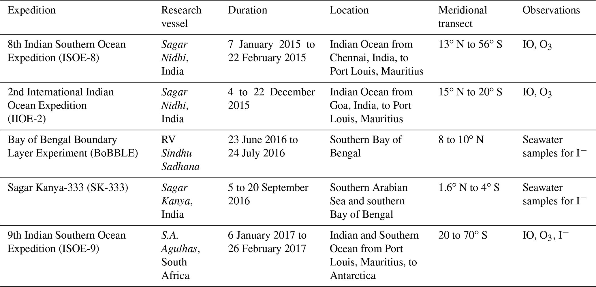
Table 2List of existing global (italicised reference column) and new region-specific (regular font in reference column) parameterisations for sea surface iodide concentration indicating data location and number of data points used to formulate each equation. Here [iodide] represents the sea surface iodide concentration (nM), and sea surface temperature is SST (in degrees Celsius for Eqs. (1) to (3) and in Kelvin for Eqs. 4 to 5). The nitrate concentration is given in micromoles (µM), the mixed layer depth is MLDpt in metres, the subscript “pt” indicates potential temperature implying a temperature change of 0.5 ∘C from the ocean surface (Monterey and Levitus, 1997), and salinity is in practical salinity units (PSU). Further details on individual parameters and the choice of Eq. (1) over others proposed in Chance et al. (2014) are discussed in the Supplement. R2∗ represents the initial coefficient of determination (COD) while deriving each parameterisation, and R2 represents the COD from correlation analysis of the calculated iodide with observations in this study (ISOE-9, SK-333, BoBBLE).
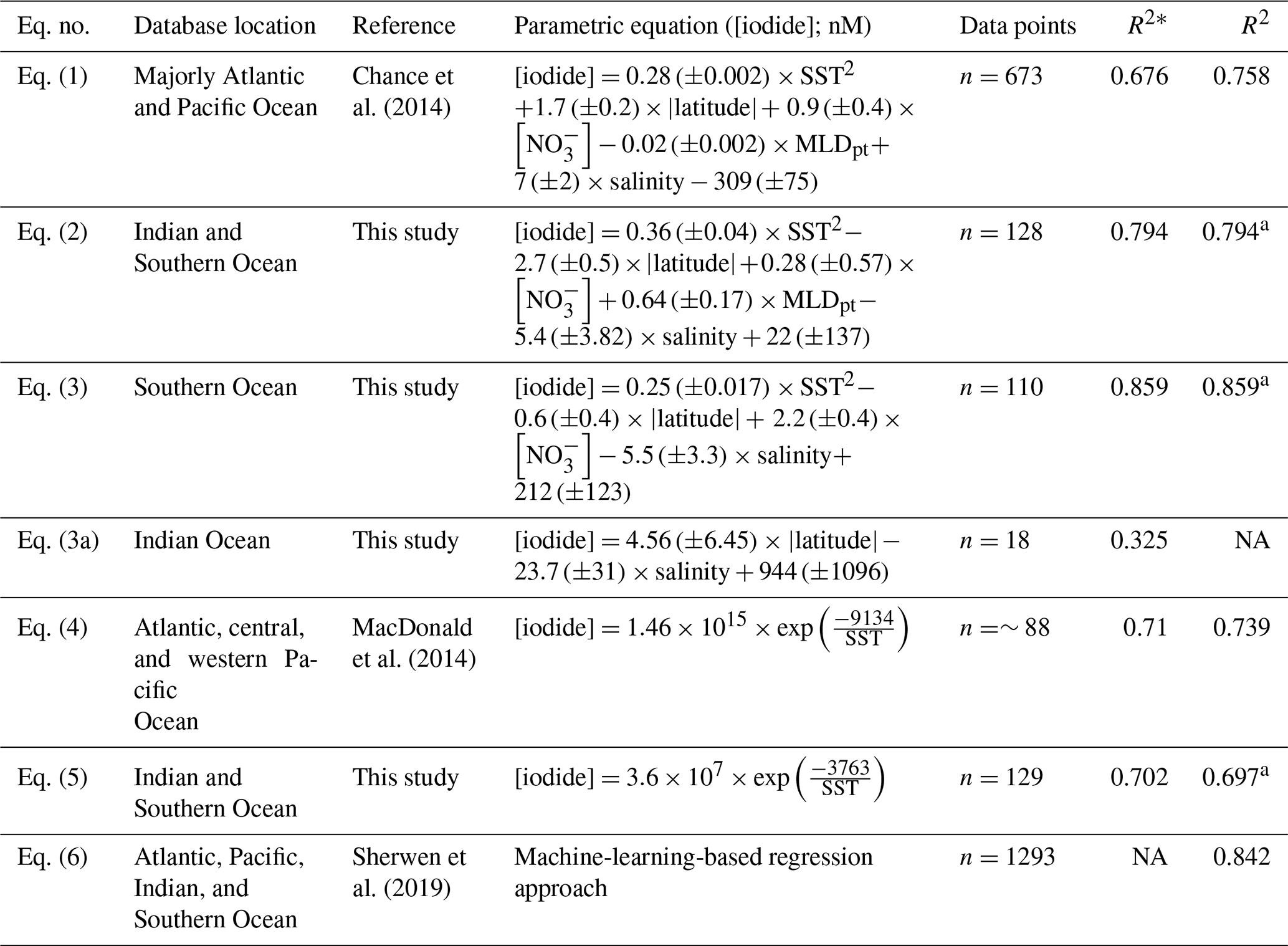
a Higher R2 values for the modified parameterisations reflect the fact that they have been derived using the same observational data as they are tested on.
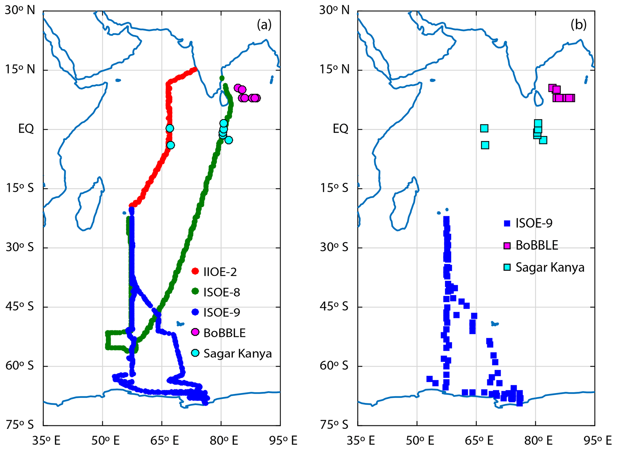
Figure 1Map of the Indian Ocean and the Southern Ocean (a) with cruise tracks for campaigns conducted during the austral summer of 2014–2016. Green circles indicate the cruise track for ISOE-8, red circles show the cruise track for IIOE-2, and blue circles indicate the cruise track for ISOE-9. Magenta and cyan circles indicate sample locations for the BoBBLE and SK-333 expeditions, respectively. (b) Boxes represent 129 seawater iodide sampling locations from three expeditions following the colour code in (a).
The 9th Indian Southern Ocean Expedition (ISOE-9) was conducted from January to February 2017 in the Southern Ocean and the Indian Ocean sector of the Southern Ocean. The expedition started from Port Louis, Mauritius, and spanned the remote open-ocean area to the coast of Antarctica. Observations of IO, SSI, and O3 were made along the cruise track during ISOE-9. For further analysis we also include IO observations from the 2nd International Indian Ocean Expedition (IIOE-2) and the 8th Indian Southern Ocean Expedition (ISOE-8) conducted in the Indian and Southern Ocean region during austral summer of 2015 (Mahajan et al., 2019a, b). We also include SSI observations in the northern Indian Ocean from two expeditions, namely the Sagar Kanya-333 cruise (SK-333) and the Bay of Bengal Boundary Layer Experiment (BoBBLE) conducted during June–July and September 2016, respectively (Chance et al., 2020). Table 1 shows the details of the expeditions, including the locations, dates of the expeditions, and the meridional transect for each expedition. Figure 1a shows a map with the cruise tracks for the five expeditions. Figure 1b shows the seawater iodide sampling locations during the ISOE-9, SK-333, and BoBBLE expeditions. The track of the ship during ISOE-9, along with the air mass back trajectories arriving at noon each day, is given in the Supplement in Fig. S1. The HYbrid Single-Particle Lagrangian Integrated Trajectory (HYSPLIT) model (Rolph et al., 2017; Stein et al., 2015) was used to calculate the back trajectories. Similar back-trajectory plots and full cruise tracks for ISOE-8 and IIOE-2 are given in Mahajan et al. (2019a, b). During the three expeditions, meteorological parameters of the ocean and atmosphere were measured using an on-board automatic weather station (WeatherPak®-2000 v3), which is specially built for shipboard observations and manual observation techniques. The WeatherPak system was installed in the front of the ship, with the sensors approximately 10 m from the sea surface. The weather system is equipped with a GPS system for measuring the true wind speed and direction along with the apparent data. The SST and salinity were measured manually through bucket sampling.
2.1 Sea surface iodide (SSI)
In this section, we focus on developing a region-specific parameterisation for SSI estimation by adapting previously established methods. The SSI concentrations obtained from the original and newly developed region-specific parameterisation as well as SSI model predictions are used for a comparison study and to calculate the inorganic iodine emissions.
2.1.1 Observed SSI in the Indian Ocean and the Southern Ocean
Historically, few observations of SSI are available for the Indian Ocean basin, with reports of only three data points in the open ocean from the Arabian Sea sector of the Indian Ocean (Farrenkopf and Luther, 2002). Two of these values are coastal, and they lack supporting sea surface temperature and salinity data; thus, they have been excluded from this study. However, recent work has led to a large increase in the number of SSI observations available for the Indian Ocean and Southern Ocean (Indian Ocean sector) (Chance et al., 2020). Specifically, 111 new observations were made during the 2016 ISOE-9 and 18 during the SK-333 and BoBBLE. During the ISOE-9, SSI measurements in seawater were made concomitant with observations of O3 and IO in the gas phase for the first time. Observations of SSI made during this expedition used the cathodic stripping voltammetry method with a hanging mercury drop electrode as a working electrode (Campos, 1997; Luther et al., 1988). The errors reported on the concentrations reflect the standard deviation of the repeat scans and the standard error on the intercept and slope of the calibration. The seawater samples were collected during the ISOE-9 at a 3–6 h interval between 23 and 70∘ S. Seawater samples from the SK-333 cruise and BoBBLE were analysed following the same technique for surface iodide concentrations. Iodide data from SK-333 and BoBBLE contributed to 18 additional data points between 10∘ N and 4∘ S, making a total of 129 new locations (excluding coastal and extremely high values above 400 nM; see Chance et al., 2020, for details) for observed SSI in the Indian Ocean and Southern Ocean region. This is a major sample size compared to the global 2014 database (n=925) across all the global oceans (Chance et al., 2014), and these data points contribute substantially to the recently updated iodide dataset (Chance et al., 2019) (n=1342). From here onwards, the iodide concentrations obtained from sampling observations will be referred to as measured SSI as opposed to modelled SSI to differentiate between the observed iodide concentrations and those calculated using the parameterisations. All available observations made in the Indian Ocean basin as presented in Chance et al. (2019) have been included for the development of the region-specific parameterisation presented in this work. Further details about the measurement technique and the observations used can be found in Chance et al. (2020).
2.1.2 Iodide parameterisations
Due to the sparsity of SSI measurements, different empirical parameterisations have been proposed to estimate SSI concentrations. Parameters like SST and salinity (only for SK-333 and BoBBLE; R2=0.3, P=0.018) show a positive correlation with SSI concentrations. However, a global parameterisation scheme may not capture the specificities of these required for regional studies. The northern Indian Ocean has markedly different sea surface salinity (D'Addezio et al., 2015) and SST (Dinesh Kumar et al., 2016) in its two basins, the Arabian Sea and the Bay of Bengal, that share the same latitude bands separated by the Indian subcontinental land mass. These basins experience the biannually reversing monsoonal winds, which greatly influence their SST and salinity structure. Strong winds in the Arabian Sea associated with the summer monsoon dissipate heat via overturning and turbulent mixing, whereas weaker winds in the Bay of Bengal imply high SST due to the formation of a stable and shallow surface mixed layer (Shenoi, 2002). The Arabian Sea exhibits much higher salinity compared to the Bay of Bengal due to greater evaporation and lower river runoff (Rao and Sivakumar, 2003). As mentioned earlier, the current global SSI parameterisations are based almost entirely on observations from the Atlantic, Pacific, and Southern Ocean and have not been tested in the Indian Ocean region.
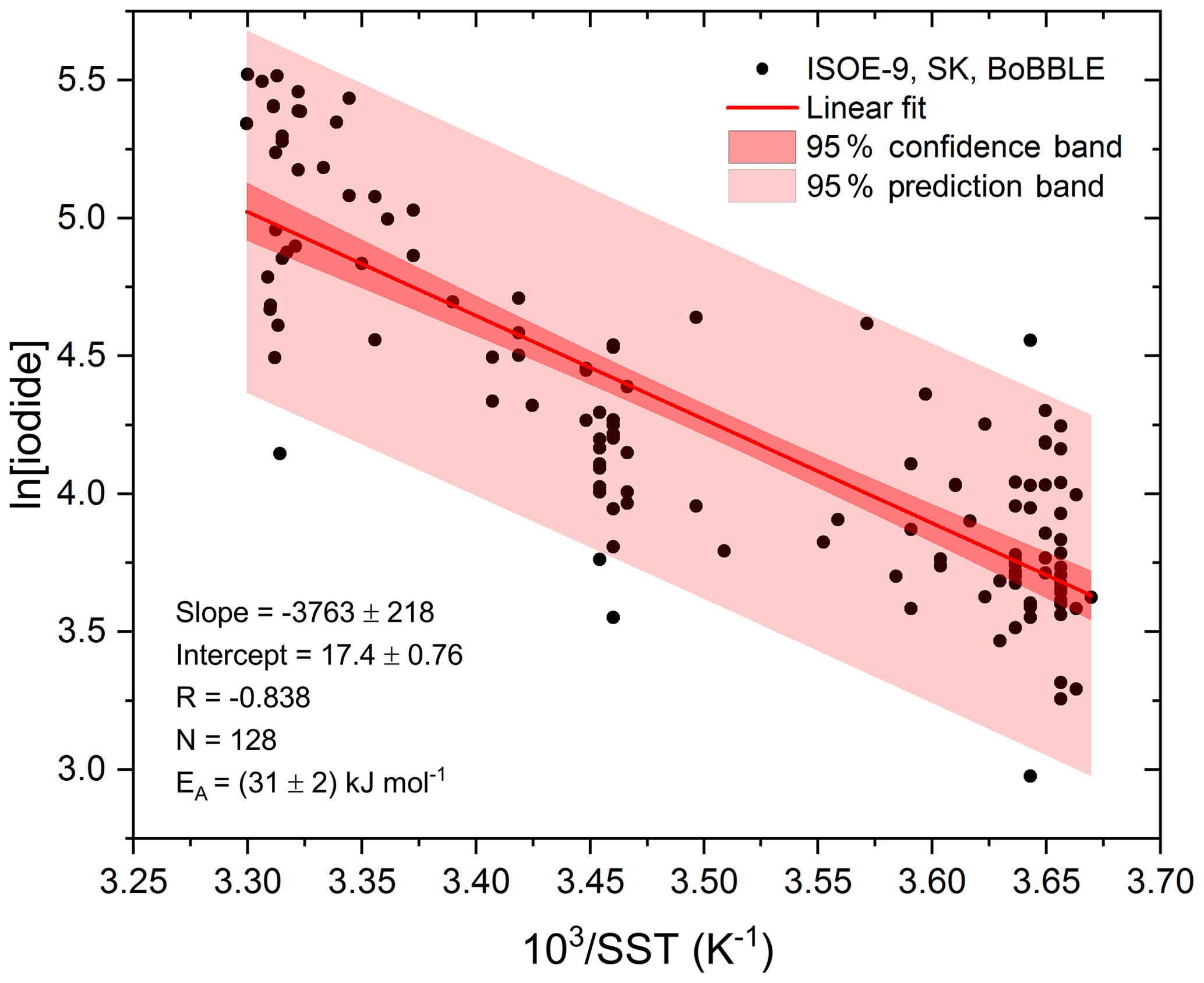
Figure 2Arrhenius form plot of sea surface iodide concentrations against SST from all available seawater iodide field observations in the Indian Ocean and Southern Ocean. The red line represents a linear fit; the shaded region in dark red (inner) indicates the 95 % confidence bands, and the shaded area in light red (outer) indicates the 95 % prediction bands.
Here, we aim to create region-specific parameterisations for the Indian and Southern Ocean and conduct a comparison between these and the existing global parameterisations, further discussed in Sect. 4.2. The existing (Eqs. 1, 4, and 6) global and the new region-specific parameterisations are listed in Table 2. Below we briefly describe the modified parameterisations. Details about the original parameterisations can be found in their respective publications (Chance et al., 2014; MacDonald et al., 2014; Sherwen et al., 2019).
- a.
Linear regression analysis was performed on each parameter, namely SST, mixed layer depth (MLD), latitude, sea surface nitrate concentration (as it has been suggested that iodate could be reduced by nitrate-based enzymes; Chance et al., 2014), and salinity, against the measured SSI concentrations from the ISOE-9, SK-333, and BoBBLE campaigns, similar to the Chance et al. (2014) technique but using in situ SST and salinity observations instead of climatological values. More details on the approach taken can be found in the Supplement. The combination with the largest R2 and a uniform distribution of residuals from the statistically significant dependent variables, as detailed in Table S1, resulted in Eq. (2) in Table 2. Equation (2) thus represents a region-specific (the Indian Ocean and Southern Ocean region abbreviated as Ind. O. + Sou. O. in the figures) variant of the Chance et al. (2014) parameterisation for the estimation of SSI concentrations. Similarly, keeping in mind the difference in the SST and salinity for the Indian Ocean and Southern Ocean, another parameterisation was derived only for the Southern Ocean region using the ISOE-9 iodide observations and for the Indian Ocean using the SK-333 and BoBBLE iodide observations, respectively. The parameterisation for the Southern Ocean region using ISOE-9 iodide observations is given in Table 2 as Eq. (3). A similar Indian Ocean parameterisation is formulated and listed in the last row of Table 2 as Eq. (3a). However, this parameterisation is not valid, and it is omitted from analysis in this text due to statistical insignificance inferred from an analysis of variance (ANOVA) test using StatPlus statistical analysis software. In this method, the F ratio from ANOVA analysis is compared with the critical F value from the standard f-distribution table (at 0.05 significance level) to confirm the statistical robustness. Results of the ANOVA test on the datasets for Eqs. (2), (3), and (3a) are discussed in the Supplement.
- b.
A second method for the estimation of SSI concentration was proposed by MacDonald et al. (2014) that uses the correlation between sea surface iodide and SST. At present, this is the most commonly used parameterisation in global models (Sherwen et al., 2016c, b, a; Stone et al., 2018). Similar to MacDonald et al. (2014) (Table 2, Eq. 4), we derived an Arrhenius-type, region-specific expression using iodide and SST data from ISOE-9, SK-333, and BoBBLE. Figure 2 shows the typical linear dependence of ln[I−] for observed SSI in the Indian Ocean and Southern Ocean, with SST−1, which resulted in the Arrhenius form expression given as Eq. (5) in Table 2.
Figure 3 shows the iodide concentrations for the three campaigns, ISOE-8, IIOE-2 and ISOE-9, calculated using Eqs. (1) to (5), the measured iodide concentrations from ISOE-9, SK-333, and BoBBLE, and the global iodide model predictions obtained from Sherwen et al. (2019) (Table 2). From here on, region-specific parameterisations developed for SSI concentrations are referred to as the modified versions of the original parameterisations; Eqs. (2) and (3) are called the modified Chance et al. (2014) parameterisation for the Indian Ocean and Southern Ocean region and only the Southern Ocean region, respectively. Equation (5) is called the modified MacDonald et al. (2014) parameterisation. The machine-learning-based model proposed in Sherwen et al. (2019) is referred to as the “SSI model”.

Figure 3Latitudinal averages of calculated sea surface iodide (SSI) concentrations for each campaign using (a) existing and (b) new parameterisation tools and observations from ISOE-9, SK-333, and BoBBLE. Filled markers represent combined SSI from ISOE-8 and ISOE-9; unfilled markers represent SSI from the IIOE-2 campaign.
2.2 Ozone
Surface ozone was monitored using a US EPA approved nondispersive photometric UV analyser (Ecotech EC9810B) installed on the ship during the expeditions to detect surface ozone values at a 1 min temporal resolution. A Teflon tube ∼4 m long fixed towards the front of the ship acted as an inlet for the analyser. The analyser is equipped with a selective ozone scrubber, which was alternatively switched in and out of the measuring stream. The analyser has a lower detection limit of 0.5 ppbv and a precision of 1 ppbv. A 5 µm polytetrafluoroethylene (PTFE) filter membrane installed in the sample inlet tube was changed regularly. Zero and span calibrations were done every alternate day to ensure accurate O3 measurements. The ozone data collected were cleaned to remove the data points under the influence of the ship's smokestack by referring to the measured apparent wind direction on the ship. Apparent wind approaching the ship from 0 to 90∘ or 27 to 360∘ (front hemisphere of the ship) was considered free from smokestack emission influence; 0 or 360∘ represents the bow of the ship. Ozone data recorded when the ship was stationary showed major smokestack emission influence and were excluded.
2.3 Estimation of inorganic iodine fluxes
In order to estimate the contribution of inorganic iodine chemistry to active iodine chemistry in the atmosphere, the atmospheric fluxes for the main product species, I2 and HOI, need to be calculated, since direct flux measurements of I2 and HOI have not been done anywhere in the world to date. While there are reported observations of marine I2 emissions, they are few in number and mostly from coastal regions (Atkinson et al., 2012; Huang et al., 2010; Saiz-Lopez et al., 2006) with one observation in the open ocean (Lawler et al., 2014), although these are all observations of atmospheric concentrations and not fluxes. As observed SSI is not available for all cruises, we used the following scenarios for SSI to estimate the inorganic iodine fluxes:
- a.
using measured SSI from observations of sea surface iodide from ISOE-9, SK-333, and BoBBLE;
- b.
using calculated SSI from
- 1.
the Chance et al. (2014) parameterisation in Eq. (1),
- 2.
the modified Chance et al. (2014) parameterisation for the Indian Ocean and Southern Ocean (Ind. O. + Sou. O.) in Eq. (2),
- 3.
the modified Chance et al. (2014) parameterisation for the Southern Ocean (Sou. O.) in Eq. (3),
- 4.
the MacDonald et al. (2014) parameterisation using SST in Eq. (4),
- 5.
the modified MacDonald et al. (2014) parameterisation in Eq. (5), and
- 6.
a machine-learning-based model prediction (Sherwen et al., 2019) in Eq. (6).
- 1.
Ozone was measured on all three cruises (ISOE-9, IIOE-2, and ISOE-8). The fluxes for HOI and I2 were then calculated for all the above scenarios except for the observations from SK-333 and BoBBLE as IO observations were not taken during these cruises. The following algorithm was used for estimating iodine fluxes (Carpenter et al., 2013):
where the fluxes are in nanomoles per square metre per day (nmol m−2 d−1), [O3] is in nanomoles per mole (nmol mol−1) (ppbv), [I−] in moles per cubic decimetre (mol dm−3), and the wind speed (WS) is in metres per second (m s−1). Carpenter et al. (2013) did not consider the effect of temperature in the interfacial layer of the sea surface model on activation energies for the Reaction (R1) (i.e. assumed the temperature dependence for k (I− + O3) to be zero). Although I2 and HOI fluxes are expected to increase with the temperature of the interfacial layer, I2 production has a negative activation energy, as noted by MacDonald et al. (2014). In Carpenter et al. (2013) (specific to the tropical Atlantic), a seawater temperature of 15 ∘C and air temperature of 20 ∘C were used to calculate Henry's law constants, diffusion constants, and mass transfer velocities. Again assuming the temperature dependence of k(I− + O3) to be zero but including the temperature dependence of Henry's law constants, diffusion constants, and mass transfer velocities, the same interfacial layer model predicted effective activation energies for I2 and HOI emissions of −2 and 25 kJ mol−1 (MacDonald et al. (2014). Using these activation energies, MacDonald et al. (2014) calculated differences in I2 and HOI fluxes of 3 % and 31 %–41 %, respectively, at SSTs of 10 and 30 ∘C compared to the room-temperature parameterisations presented in Carpenter et al. (2013). Experimentally derived activation energies for I2 and HOI emissions were −7 ± 18 and 17±50 kJ mol−1 (MacDonald et al., 2014). As HOI represents the larger iodine flux, the higher relative uncertainty in the activation energy should be kept in mind when calculating temperature-dependent emissions. It should be noted that a recent study suggested that the activation energies from MacDonald et al. (2014) are better summarised as approximately zero (e.g. Moreno and Baeza-Romero, 2019) as the overall temperature dependence remains unresolved.
HOI and I2 fluxes are also influenced by the wind speed as seen from Eqs. (7) and (8), and the modelled iodine fluxes (HOI and I2) are highest for high [O3], high [I−], and low wind speed. This is explained by the assumption that wind shear drives mixing of the interfacial layer to bulk seawater, reducing the efflux of HOI and I2 into the atmosphere (Carpenter et al., 2013). Negative fluxes are obtained from Eqs. (7) and (8) for both HOI and I2 when the wind speed is higher than 14 m s−1, which is not physically possible, and therefore the model output is limited to wind speeds below 14 m s−1 (Mahajan et al., 2019a). Iodine fluxes calculated from Eqs. (7) and (8) using SSI concentrations from the scenarios (a) and (b: 1–6) are shown in Fig. 4c and d.
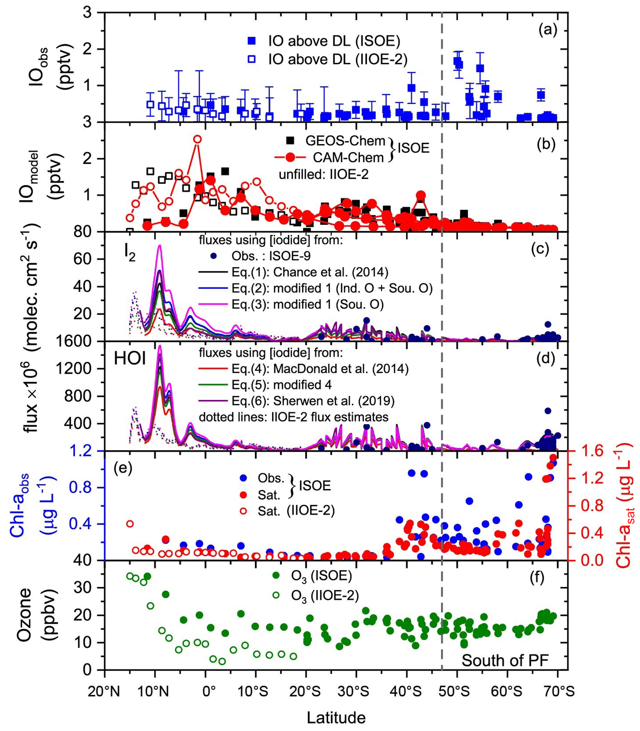
Figure 4Daily averaged atmospheric and oceanic parameters combined from the ISOE-8, IIOE-2, and ISOE-9 field campaigns. Data marked with “ISOE” represent combined data from ISOE-8 and ISOE-9. Unfilled markers and dotted lines show values for IIOE-2. (a) IO above the detection limit from ISOE-8, ISOE-9. and IIOE-2. (b) Surface IO values from the GEOS-Chem and CAM-Chem models. Panels (c) and (d) comprise HOI and I2 fluxes estimated from Eqs. (7) and (6), respectively. Fluxes are colour-coded for different sea surface iodide (SSI) datasets used for their estimation. Black, blue, red, and green correspond to fluxes calculated using SSI estimation from Eqs. (1) to (5); purple represents the use of model SSI predictions (Sherwen et al., 2019), and filled circles in dark blue correspond to measured SSI from ISOE-9 for each observation. (e) Chlorophyll a observations from ISOE-8 and ISOE-9 (blue circles) as well as satellite data for all campaigns (red circles). (f) Ozone mixing ratios from campaigns ISOE and IIOE-2. The dashed line marks the polar front at 47∘ S. Observational plots for ISOE-8 and IIOE-2 were adapted from Mahajan et al. (2019a, b). The vertical dashed line through the figure indicates the PF (polar front).
2.4 Iodine oxide
2.4.1 Observations
Ship-based measurements of IO were made using the multi-axis differential optical absorption spectroscopy (MAX-DOAS) technique (Hönninger et al., 2004; Platt and Stutz, 2008). The MAX-DOAS device was installed at the bow of the ship with a direct line of sight towards the front of the ship to avoid the ship's plume in the detection path of the telescope. The MAX-DOAS device was programmed to capture scattered sunlight spectra every 1 s at set elevation angles of 0, 1, 2, 3, 5, 7, 20, 40, and 90∘ during daylight hours. Mercury line calibration offset and dark current spectra were recorded after sunset each day. Elevation angles outside a range of ±0.2∘ from the set value were eliminated from the 30 min averaged spectra for increased accuracy. Figure S2 shows the resultant IO and O4 differential slant column densities (DSCDs) for the ISOE-9 campaign; similar plots are available for ISOE-8 (Mahajan et al., 2019a) and IIOE-2 (Mahajan et al., 2019b). The QDOAS software (Danckaert et al., 2017) was used for DOAS retrieval of IO from the spectra using the optical density fitting analysis method. The spectra were fitted with a third-order polynomial using a fitting interval of 415 to 440 nm with cross sections of NO2 (Vandaele et al., 1998), O3 (Bogumil et al., 2003), O4 (Thalman and Volkamer, 2013), H2O (Rothman et al., 2013), two ring spectra, first as recommended by Chance and Spurr (1997) and second following Wagner et al. (2009), and a liquid water spectrum for seawater (Pope and Fry, 1997). To remove the influence of stratospheric absorption a spectrum corresponding to 90∘ (zenith) from each scan was used as a reference for the analysis. The raw spectra were analysed to obtain differential slant column densities (DSCDs), and values with a root mean square error (RMSE) greater than 10−3 were eliminated. Similarly, DOAS retrieval of O4 in the 350 to 386 nm spectral window was performed, and DSCDs were obtained. The optical density fits for IO and O4 from ISOE-9 are shown in Fig. S3. The IO DSCDs were then converted to volume mixing ratios using the O4 slant columns following the previously used “O4 method” (Mahajan et al., 2012; Prados-Roman et al., 2015; Sinreich et al., 2010; Wagner et al., 2004). Further details on the instrument, retrieval procedure, and conversion into mixing ratios can be found in previous works (Mahajan et al., 2019a, b).
2.4.2 Modelled atmospheric IO
We use outputs from two global models for a comparison with the observations conducted during the three cruises. The first model is the GEOS-Chem chemical transport model (version 10-01, 4×5∘ horizontal resolution, http://www.geos-chem.org, last access: 1 April 2019), which includes detailed HOx–NOx–VOC–ozone–halogen–aerosol (VOC: volatile organic carbon) tropospheric chemistry (Sherwen et al., 2016c, 2017) and is driven by offline meteorology from the NASA Global Modelling and Assimilation Office (http://gmao.gsfc.nasa.gov, last access: 5 April 2019) forward processing product (GEOS-FP).
The second model is the 3D chemistry–climate model CAM-Chem version 4 (Community Atmospheric Model with Chemistry) https://www2.acom.ucar.edu/gcm/cam-chem, last access: 8 April 2019), which is included in the CESM framework (Community Earth System Model, CAM-Chem, version 4.0). The model includes a state-of-the-art halogen chemistry scheme (chlorine, bromine, and iodine) (Saiz-Lopez and Fernandez, 2016). The current configuration includes an explicit scheme for organic and inorganic iodine emissions and photochemistry. These halogen sources comprise the photochemical breakdown of five very short-lived bromocarbons (CHBr3, CH2Br2, CH2BrCl, CHBrCl2, and CHBr2Cl) naturally emitted by phytoplankton from the oceans (Ordóñez et al., 2012). The model was run in specified dynamic mode (Ordóñez et al., 2012), with a spatial resolution of 1.9∘ latitude by 2.5∘ longitude and 26 vertical levels from the surface to up to 40 km.
Both models include biotic emissions of four iodocarbons (CH3I, CH2ICl, CH2IBr, and CH2I2) as described by Ordóñez et al. (2012) and abiotic oceanic sources of HOI and I2 based on the Carpenter et al. (2013) and MacDonald et al. (2014) laboratory studies of the oxidation of aqueous iodide by atmospheric ozone at the ocean surface. Both models here use the MacDonald parameterisation expression (Eq. 4; MacDonald et al., 2014) discussed in Sect. 2.1.2 to predict surface iodide used for calculating iodine emissions and the organo-halogen emissions from Ordóñez et al. (2012). IO surface concentrations for the three campaigns (IIOE-2, ISOE-8, and ISOE-9) were extracted from the model runs and used for comparison. Currently, these two global models include reactive iodine chemistry (along with TOMCAT, which includes the tropospheric iodine chemistry; Hossaini et al., 2016).

Figure 5Latitudinal plot of hourly averaged field measurements of wind speed, ozone mixing ratios, SST, and salinity (salinity data for IIOE-2 are monthly climatological means from the World Ocean Atlas as described in the Supplement) from the ISOE-8, IIOE-2, and ISOE-9 campaigns. Data markers in red are for the IIOE-2 campaign; those in blue are for ISOE-8, and markers in black are from ISOE-9 for all the panels. Observational plots for ISOE-8 and IIOE-2 were adapted from Mahajan et al. (2019a, b).
3.1 Ozone, meteorological, and oceanic parameters
The latitudinal distributions of hourly average values of U10 wind speed (WS), O3, SST, and salinity from all the campaigns are shown in Fig. 5. Winds arriving at the ship, shown in Fig. 5a, remained low for most of the duration of all three expeditions, with wind speed ranging from 1 m s−1 to stronger winds of 24 m s−1 on a few days. Even stronger winds (above 30 m s−1) were observed during ISOE-9 in the region between 64 and 65∘ S, with the highest wind speed of 32 m s−1 at 66∘ S on the night of 8 February 2017. Ozone mixing ratios (Fig. 5b) during all three expeditions showed a similar trend, exhibiting a large reduction in values in the open-ocean environment compared to coastal environments. The back trajectories (Supplement) show that for most of the expeditions, air masses arriving at the cruise location were from the open-ocean environment and did not have any anthropogenic influence for the last 5 d. This is reflected in the O3 values, which range between 8 and 20 ppbv in the open ocean but were between 30 and 50 ppbv near the coastal regions, where the air mass back trajectories confirm anthropogenic origins. Close to the Indian Subcontinent ozone levels peaked at about 50 ppbv during ISOE-8. They also showed a distinct diurnal variation, with higher ozone values during the daytime due to photochemical production. However, in the open-ocean environment, ozone mixing ratios did not show this diurnal variation, and indeed values of ozone dropped during daytime, indicating photochemical destruction during both ISOE-8 and ISOE-9 (Fig. 5b).
As already noted, SST is widely used to predict SSI (Eqs. 4 and 5). Combined SST data (Fig. 5c) reveal a steady decrease in sea surface temperature from 15 to 68∘ S for all the campaigns. During January 2015 (ISOE-8) seawater north of 6∘ N displays slightly lower SST (∼3 ∘C) compared to that in December 2015 (IIOE-2). Salinity is also an important parameter for the prediction of SSI (higher coefficient in Eqs. 1, 2, and 3). The Southern Ocean region explored during ISOE-8 and ISOE-9 reveals similar salinity values (Fig. 5d) for the austral summer months of 2015 and 2016 (January–February). The salinity data show relatively lower values for ISOE-8 compared to those for IIOE-2 for the region 15∘ N to 20∘ S. Despite the inter-annual differences in the northern Indian Ocean region, salinity values of ∼35 PSU overlap for IIOE-2 and ISOE-8 in a small window of 7∘ N to the Equator. Below the Equator, the salinity values for IIOE-2 increase, while for ISOE-8 salinity remains lower than 35 PSU until 20∘ S. Seawater between 20 and 44∘ S has a nearly constant salinity of 35 PSU, which decreases to ∼33.5 PSU after 44∘ S and remains the same until 65∘ S after which the salinity begins to drop to 31.5 PSU near 67∘ S close to Antarctica.
3.2 Sea surface iodide concentration
Latitudinal averages of SSI concentrations estimated from seven scenarios (listed in Sect. 2.3) are shown in Fig. 3. SSI estimates from the IIOE-2 campaign are marked separately to differentiate them from the ISOE estimates for the Indian Ocean region. There is a clear difference in the estimated SSI in different scenarios. All the estimates and the model follow a similar pattern, showing elevated levels in the tropics compared to the higher latitudes. SSI estimates from parameterisations (Eqs. 1, 3, 4, and 5) show nearly constant values for SSI from 15∘ N to 25∘ S, after which a steady decline is noted until 70∘ S. Thus, the parameterisations based on Eqs. 1, 3, 4, and 5 do not capture the decreasing trend observed for iodide around the Equator. Equation (2), which was derived specifically for the Indian Ocean and Southern Ocean region, better captures this trend and also shows a better match to the measured SSI from SK-333 and BoBBLE in the Indian Ocean. Equation (6) also predicts lower concentrations around the Equator than in the northern Indian Ocean. SSI concentrations estimated using the Chance et al. (2014) parameterisation (Eq. 1) show a small increase in iodide concentrations south of 47∘ S (polar front), which is not observed in the other parameterisations, but there is some suggestion of an increase in the observations. Equation (1) also resulted in a large difference (∼50 nM) of SSI estimates north of 10∘ N between the IIOE-2 and ISOE-8 cruises, while this difference was lower for the other parameterisations. This difference between the SSI estimates for the IIOE-2 and ISOE-8 cruises is due to the large difference in salinity values for this region (Sect. 4.1). SSI estimates using Eq. (2) show good agreement with the model prediction of Sherwen et al. (2019), both indicating a decrease in SSI concentrations near the Equator during the IIOE-2 and ISOE-8 expeditions. Some high SSI concentrations (up to ∼250 nM) were observed around 10∘ N; these were best replicated by Eq. (3). The highest SSI concentrations estimated using Eq. (3) were 244 nM at 7∘ N during IIOE-2 and 242 nM at 12∘ S during ISOE-8. At the Equator, Eq. (2) performs better in predicting the SSI concentrations, with a difference of ∼75 nM compared to the observations. SSI estimates from Eq. (4), i.e. the MacDonald et al. (2014) parameterisation, were lower than the measured iodide concentrations and all other parameterisation, including the model (Eq. 7) predictions. Overall, all modified parameterisations (Eqs. 2, 3, and 5) estimate higher SSI compared to the original parameterisation (Eqs. 1 and 4), with the exception of the region south of 20∘ S, where Eq. (3) predicts lower SSI than Eq. (1). The modified MacDonald parameterisation (Eq. 5) estimated iodide concentrations to be greater by 50 nM for the entire dataset in comparison to the existing MacDonald parameterisation given by Eq. (4). For Eq. (5), the uncertainty in the iodide concentration from the 95 % prediction band is ∼15 % of the predicted value.
3.3 Iodine fluxes
Figure 4 shows the latitudinal variation in IO mixing ratios, inorganic iodine emissions (HOI and I2), chl a, and ozone mixing ratios for the entire dataset comprising the three campaigns. All the panels in Fig. 4 are plots of daily averaged values during each expedition, except for the HOI and I2 fluxes; these are latitudinal averages from each campaign. Emissions calculated using the measured SSI concentrations (represented by filled spheres in Fig. 4c, d) from ISOE-9 correspond to the data points of the measured SSI concentration. Oceanic inorganic iodine emission fluxes of HOI and I2 were estimated using the Carpenter et al. (2013) parameterisation given in Eqs. (7) and (8) limited to wind speeds below 14 m s−1. Thus, the fluxes estimated from the measured SSI concentrations were reduced to 56 points (out of 111 measured SSI data points). The seven different datasets of iodide concentrations (listed in Sect. 2.3) have been used for the estimation of HOI and I2 fluxes. For the entire dataset, the highest fluxes were obtained when using the SSI concentrations from the modified Chance et al. (2014) parameterisation (Eq. 3) derived from measured SSI in the Southern Ocean region, i.e. during ISOE-9. The second highest fluxes were estimated using SSI from Eq. (2), obtained from measured SSI in the Indian Ocean and Southern Ocean. Comparatively lower iodine emissions were estimated using SSI concentration from the MacDonald et al. (2014) parameterisation (Eq. 4). The estimated inorganic iodine fluxes in the Southern Ocean region (30∘ S and below) are much lower compared to the Indian Ocean (Fig. 5), driven by the higher estimated SSI in the latter. Maximum inorganic emissions are predicted in the tropical region, specifically north of the Equator. HOI is the dominant reactive iodine precursor species for the entire dataset, with calculated flux values 20 times higher than those for I2. Emissions estimated using SSI from Eq. (3) resulted in a peak HOI flux of 1.5×10⁹ molec. cm−2 s−1 at 9∘ N during ISOE-8. The lowest HOI flux of 1.7×10⁶ molec. cm−2 s−1 was obtained at 61∘ S during ISOE-9. For the same latitudes (9∘ N and 61∘ S), a maximum I2 flux of 7.0×10⁷ molec. cm−2 s−1 and a minimum of 1.3×10⁵ molec. cm−2 s−1 were estimated, respectively. Flux estimates from Eq. (2) are slightly lower, with a maximum HOI flux of 1.3×10⁹ and a minimum of 5.8×10⁵ molec. cm−2 s−1 as well as a maximum I2 flux of 5.2×10⁷ with a minimum of 8.3×10⁴ molec. cm−2 s−1 at the same latitudes. The estimated HOI and I2 emissions are notably lower (by ∼50 %) during IIOE-2 to the north of 5∘ S compared to emissions from ISOE-8. Between 5 and 20∘ S, the emissions from IIOE-2 and ISOE-8 are similar. Fluxes estimated using measured SSI concentrations for the ISOE-9 campaign (20 to 70∘ S) show no strong latitudinal trend for both HOI and I2 emissions. The maximum calculated HOI flux was 5.8×10⁸ molec. cm−2 s−1 at 68∘ S and the minimum was 1.1×10⁷ molec. cm−2 s−1 at 33∘ S. Similarly, I2 fluxes estimated from measured SSI concentrations peaked at 1.5×10⁷ molec. cm−2 s−1 at 32∘ S with a minimum of 3.5×10⁵ molec. cm−2 s−1 at 67∘ S. Inorganic iodine emissions estimated using model predictions for SSI concentrations from Sherwen et al. (2019) match the fluxes estimated using the iodide parameterisation tools. Despite the differences in SSI concentrations from existing and region-specific parameterisations, all result in similar values for iodine fluxes. The fluxes were calculated using the hourly wind speeds for the results to be comparable with model outputs as described below. This would result in a loss of high-temporal-resolution emission variability, but considering the frequency of the iodide and IO observations, computing the fluxes at a higher resolution will not give any extra information.
3.4 Iodine oxide
3.4.1 Observations
IO was detected above the instrument detection limit (2.1–3.5×10¹³ molec. cm−2, i.e. 0.4–0.7 pptv) in all three campaigns. The expeditions covered a track from the Indian Ocean to the Antarctic coast in the Southern Ocean and showed lower IO DSCDs in the tropics compared to the Southern Ocean, with a peak of about 3×10¹³ molec. cm−2 at 40∘ S. Figure 4a shows daily averaged IO mixing ratios for all three cruises combined. IO mixing ratios of up to 1 pptv were observed in the region 50–55∘ S, and slightly higher values of IO mixing ratios were observed in the region below 65∘ S close to the Antarctic coast. North of the polar front region, the maximum IO average mixing ratio of ∼1 pptv was observed at 40∘ S. The highest values of IO were observed close to the Antarctic coast, with up to 1.5 pptv measured during ISOE-9, and similar values are reported for the ISOE-8 expedition south of the polar front (Mahajan et al., 2019a). The IO mixing ratios in the Southern Ocean region for ISOE-9 ranged between 0.1 and a maximum of 1.57 pptv (±0.37 pptv) observed on 18 February 2017 at 50∘ S on a clear-sky day. This maximum value was observed only on 1 d and was preceded by foggy and misty days, later followed by several overcast days evidencing the role of photochemistry in IO production from its precursor gases.
3.4.2 Modelled IO
Based on the current understanding of iodine chemistry, regional and global models consider inorganic fluxes of iodine (HOI and I2) to be major contributors of iodine in the marine boundary layer. It is important to verify if the models using the existing parameterisation for these source gases can replicate observations of IO in the region of study. Thus, we have included model IO output from GEOS-Chem and CAM-Chem, both of which use the SST-based MacDonald et al. (2014) parameterisation for SSI (Fig. 4b). The surface IO output from GEOS-Chem predicts the highest levels of IO up to 1.7 pptv to the north of the Equator at 11∘ N for the time period of the IIOE-2 campaign. For the same latitudes, the model suggests lower IO levels of less than 0.5 pptv during the ISOE-8 campaign. Conversely, south of the Equator to 10∘ S, the model predicts higher IO levels during ISOE-8 and lower IO values during IIOE-2, in agreement with the observations. Below 10∘ S, IO predictions for both campaigns match well until 20∘ S, which was the latitudinal limit for the IIOE-2 campaign. To the south of 20∘ S, modelled IO levels remained below 1 pptv and exhibited a decreasing trend to the south of the polar front, in disagreement with IO observations. At locations between 40 and 43∘ S, GEOS-Chem underestimates the observed IO levels by 50 %. These locations are close to the Kerguelen Islands, and high IO values were observed here only during ISOE-8. These locations have been omitted in the correlation study between modelled and observed IO as they could be impacted by coastal or upwelling emissions, which are not well prescribed in the models.
The CAM-Chem IO surface output suggests consistently higher levels of IO during IIOE-2 compared to ISOE-8 for the same latitudinal band (Fig. 4b). Contrary to the observations, the CAM-Chem model suggests that IO levels during IIOE-2 are up to 1 pptv higher than the ISOE-8 campaign near 7∘ S latitude. The model also shows elevated IO levels of 2.7 pptv at 7.9∘ N during the IIOE-2 campaign, which does not match the observations during IIOE-2 or ISOE-8 for that region. IO levels below 1.5 pptv (11∘ N to 20∘ S) are indicated for the ISOE-8 campaign. In addition, the region between 0 and 1.5∘ S has similar IO levels for the IIOE-2 and ISOE-8 campaigns. The model predicts lower IO levels for the southern Indian Ocean and the Southern Ocean (less than 1 pptv), with decreasing IO to the south of the polar front. However, at 43∘ S, the model suggests higher IO (2.4 pptv) during ISOE-9, which matches the increase in observed IO for that region during the ISOE-8 expedition, with this region being close to the Kerguelen Islands. Both models show consistently higher absolute concentrations overall compared to the observations north of the polar front.
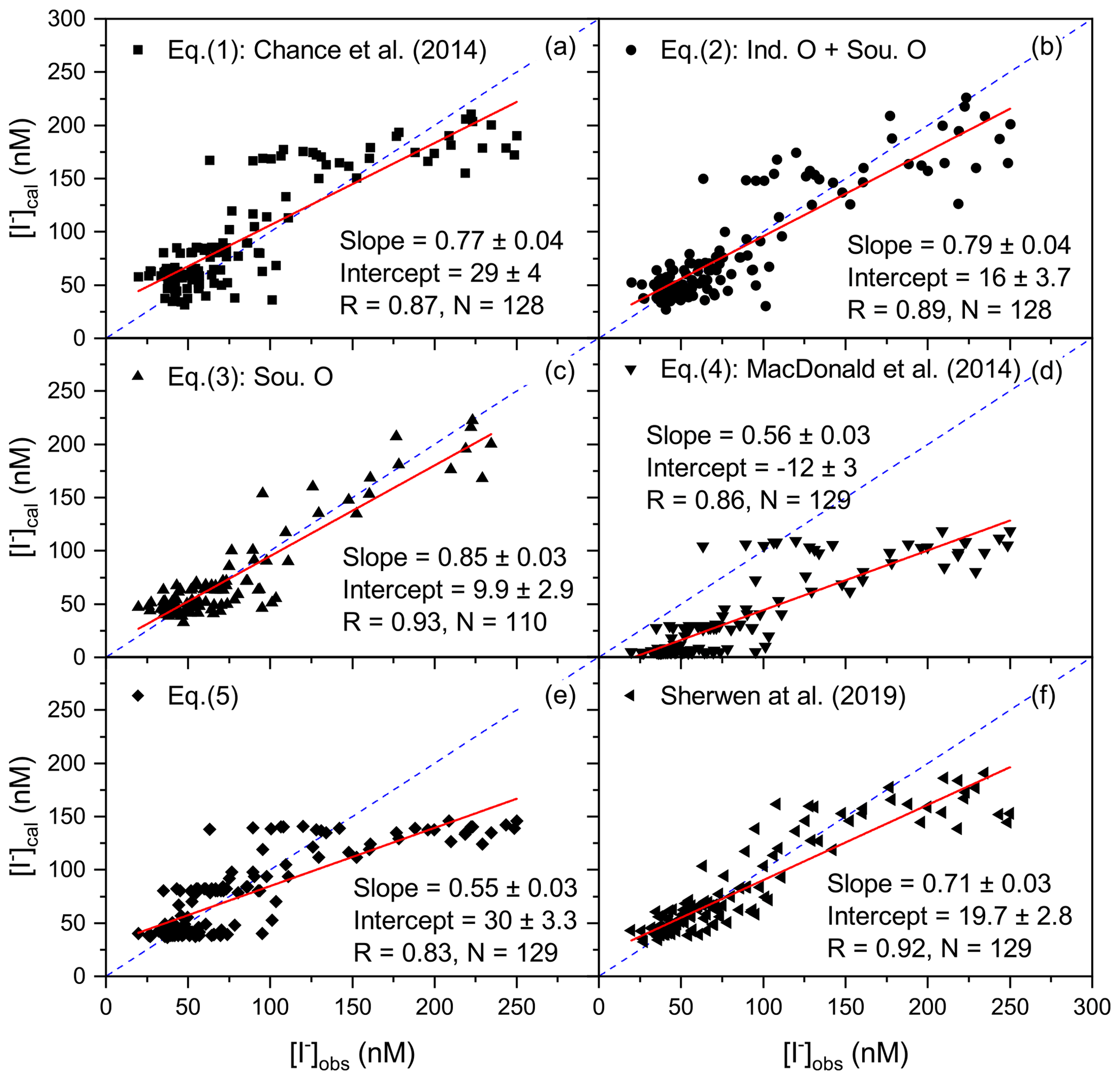
Figure 6Linear fit analysis of estimated sea surface iodide (SSI) concentrations (y axis) from parameterisation methods in Eqs. (1) to (5) and model prediction (Sherwen et al., 2019) against measured SSI concentration (x axis) from ISOE-9, SK-333, and BoBBLE. (c) SSI values are compared only with ISOE-9 observations for the Southern Ocean parameterisation. R represents the Pearson's correlation coefficient, and N is the size of the dataset. The dashed blue line represents the identity (1:1) line.
4.1 Seawater iodide
To improve the estimation of SSI in the study region, previously established parameterisations (Eqs. 1 and 4) were modified to obtain a region-specific parameterisation for SSI concentrations. SSI estimated using these modified parameterisations was less sensitive to seasonal salinity and SST changes for the northern Indian Ocean basin compared to the existing parameterisation (Fig. 3). Figure 6 shows the correlations of all the calculated SSI concentrations with the observations. The SSI estimates from Eqs. (1) to (6) correlate positively (significantly) with the measured SSI concentrations (observations) from ISOE-9 (Fig. 6). Out of the six parameterisation tools compared in this study, as expected, SSI from Eq. (2), i.e. the modified Chance equations for the Indian Ocean and Southern Ocean, showed the best correlation with the measured SSI because it was created using datasets from these campaigns (Fig. 6 and Table 2). Although the region-specific parameterisations were expected to match the observations they are based on, there was a notable difference between predictions and observations when this approach was applied only to Indian Ocean SSI measurements from SK-333 and BoBBLE (R2=0.5 for Indian Ocean parameterisation; analysis not shown). This could be attributed to the lack of SSI measurements in this region (n=18), and it highlights the fact that there may be not only seasonally but also regionally varying complexities in SSI which should be considered when estimating SSI. All parameterisation methods used for SSI estimations show that SSI concentrations are directly proportional to seawater salinity (listed in Sect. 2.3). It is evident from Figs. 5d and 3a that to the north of the Equator, the parameterisations (Eqs. 1 to 5) show lower SSI concentrations in regions with lower salinity (up to 5∘ N during ISOE-8 – filled symbols Fig. 3) and higher SSI concentrations in regions with comparatively higher salinity (during IIOE-2 – unfilled symbols Fig. 3). Only the modelled SSI concentrations using Eq. (6) (Fig. 3a, data in purple) reveal an inversely proportional relationship for salinity and SSI concentration in this region. The Sherwen et al. (2019) parameterisation (Eq. 6) produces lower SSI concentrations in high-salinity Arabian Sea waters during IIOE-2 (Fig. 3a) north of 5∘ N compared to the low-salinity Bay of Bengal waters during ISOE-8, which contradicts all the other parameterisations (Eqs. 1 to 5). Further, the SSI concentrations obtained from Sherwen et al. (2019) reverse their trend to the south of 6∘ N, with higher concentrations during IIOE-2 and lower during ISOE-8. It should be noted that only a few observations of SSI exist in this region to confirm this trend. Further discussion on the relationship between salinity and other biogeochemical variables with SSI concentrations at a global and regional scale can be found elsewhere (Chance et al., 2014, 2019).
SSI estimates considering only SST as a proxy for iodide concentration (Eq. 4) reveal positive correlations with measured SSI concentration (R=0.86, P<0.001, n=129; Fig. 6d). The modified MacDonald parameterisation (Eq. 5) also correlates positively with the measured SSI concentration but has a slightly lower coefficient of correlation (R=0.83, P<0.001, n=129; Fig. 6e). When using the SST as a proxy for SSI, a large intercept was obtained for the SSI values, evidencing the discrepancy in absolute value between this parameterisation and the observations. Equation (5) resulted in a lower intercept, approximately half of that for Eq. (4), and a lower absolute slope value of compared to the of Eq. (4) given in MacDonald et al. (2014). The lower absolute slope value for Eq. (5) implies that the SSI concentrations for this region were less sensitive to the changes in SST compared to those in Eq. (4).
Despite the lower R value, the SSI estimates from Eq. (5) in Fig. 3 are closer to the measured SSI concentration than the estimates from Eqs. (2) and (3) for the region from 25 to 70∘ S. However, north of 25∘ S, the SSI estimates from Eqs. (3) and (5) differ by ∼40 %. Both SST-based parameterisations (Eqs. 4 and 5) did not show the observed latitudinal variation in the SSI concentrations near the Equator. Linear regression of SSI with SST for only the Indian Ocean region revealed that there was no correlation between the two (R2=0.07, P=0.3, n=18). The SSI in this region only showed dependence on the salinity and latitude; correlations with the other parameters were not significant. This highlights the fact that SST may not be a very good proxy for SSI in the Indian Ocean, especially near the Equator. This is explored further in Chance et al. (2020). The original Chance et al. (2014) parameterisation displays higher sensitivity to seasonal salinity changes compared to the existing and modified parameterisation in the Indian Ocean region (Sect. 3.3). However, this method predicted an increasing iodide concentration to the south of the polar front (47∘ S), which is not supported by observations in this region (Fig. 3). In conclusion, considering the correlation with the measured SSI concentration and dependence on seawater salinity, the region-specific modified Chance parameterisation (Eq. 2) is a suitable method to estimate SSI concentration for the Indian Ocean and Southern Ocean region. The modelled SSI estimates by Sherwen et al. (2019) capture the SSI trend close to the Equator better than other existing schemes, but it fails to replicate higher SSI observations at locations 8∘ N, 40∘ S and to the south of 65∘ S close to the Antarctic coast (Fig. 3).
4.2 Atmospheric iodine
Combined IO observations from IIOE-2, ISOE-8, and ISOE-9 (Fig. 4a) show that the Indian Ocean region has comparatively less IO in its MBL than the Southern Ocean region. IO remained below 1 pptv up to 40∘ S and reached a maximum IO of 1.6 pptv south of the polar front. Modelled surface IO output from GEOS-Chem and CAM-Chem using the MacDonald et al. (2014) parameterisation (Fig. 4b) does not match the observations of IO, although they generally show good agreement with each other. The models show similar spatial patterns across the entire dataset, except for two periods of very high IO levels predicted by CAM-Chem (Fig. 4b). As well as structural differences between CAM-Chem and GEOS-Chem, there are many halogen-specific differences in rate constants, heterogeneous parameters, cross sections, and photolysis of species (e.g. higher iodine oxides) which could explain differences in predicted gas-phase IO. Considering the generally lower wind speeds and higher ozone concentrations seen in IIOE-2 versus SOE-8 and SOE-9, the calculated fluxes are higher and therefore more sensitive to assumptions, such as minimum wind speeds provided to the Carpenter et al. (2013) parameterisation. GEOS-Chem uses a minimum wind speed of 5 m s−1; however, CAM-Chem uses a minimum wind speed of 3 m s−1, and hence fluxes calculated using the surface winds in these models are expected to be slightly different.
Both models suggest higher than observed IO levels in the Indian Ocean region but underpredict IO for the Southern Ocean region. The highest detected IO levels, both in the Southern Ocean and in a narrow band around 43∘ S, were not reflected in the model predictions. We note that these occurred in regions of elevated chl a values (Fig. 4e) close to the Kerguelen Islands. Mahajan et al. (2019a) also reported positive correlations for IO with chl a for the Indian Ocean region above the polar front for a subset of the dataset (ISOE-8). Calculated fluxes of HOI and I2 (Fig. 4c and d) fail to directly explain trends in the detected IO levels for the entire dataset, regardless of the method used to estimate SSI. Maximum levels of HOI and I2 predicted to the north of 5∘ N correspond to rather low levels of IO (<0.5 pptv) in this region. However, this has been attributed to NOx titration of IO (Mahajan et al., 2019b). The models, however, do not capture this iodine titration by NOx as seen in the observations, even though the reactions of IO with NOx are included (Ordóñez et al., 2012). Similarly, for the region south of the polar front, the calculated iodine fluxes remain low in the region of the maximum detected IO concentrations during the ISOE-8 and ISOE-9 campaigns. Iodine fluxes estimated for the Indian Ocean region (15 to 5∘ N) during IIOE-2 and ISOE-8 show large differences, with much higher values during ISOE-8. However, the modelled IO is in fact higher for IIOE-2 than during ISOE-8 (5–15∘ N). Considering that the models do not reflect the fluxes, this indicates that either photochemistry or dynamical dilution of the fluxes led to this difference in the model. Additionally, the elevated levels of IO predicted in the models suggest that CAM-Chem and GEOS-Chem overestimate the impact of iodine chemistry in the northern Indian Ocean.
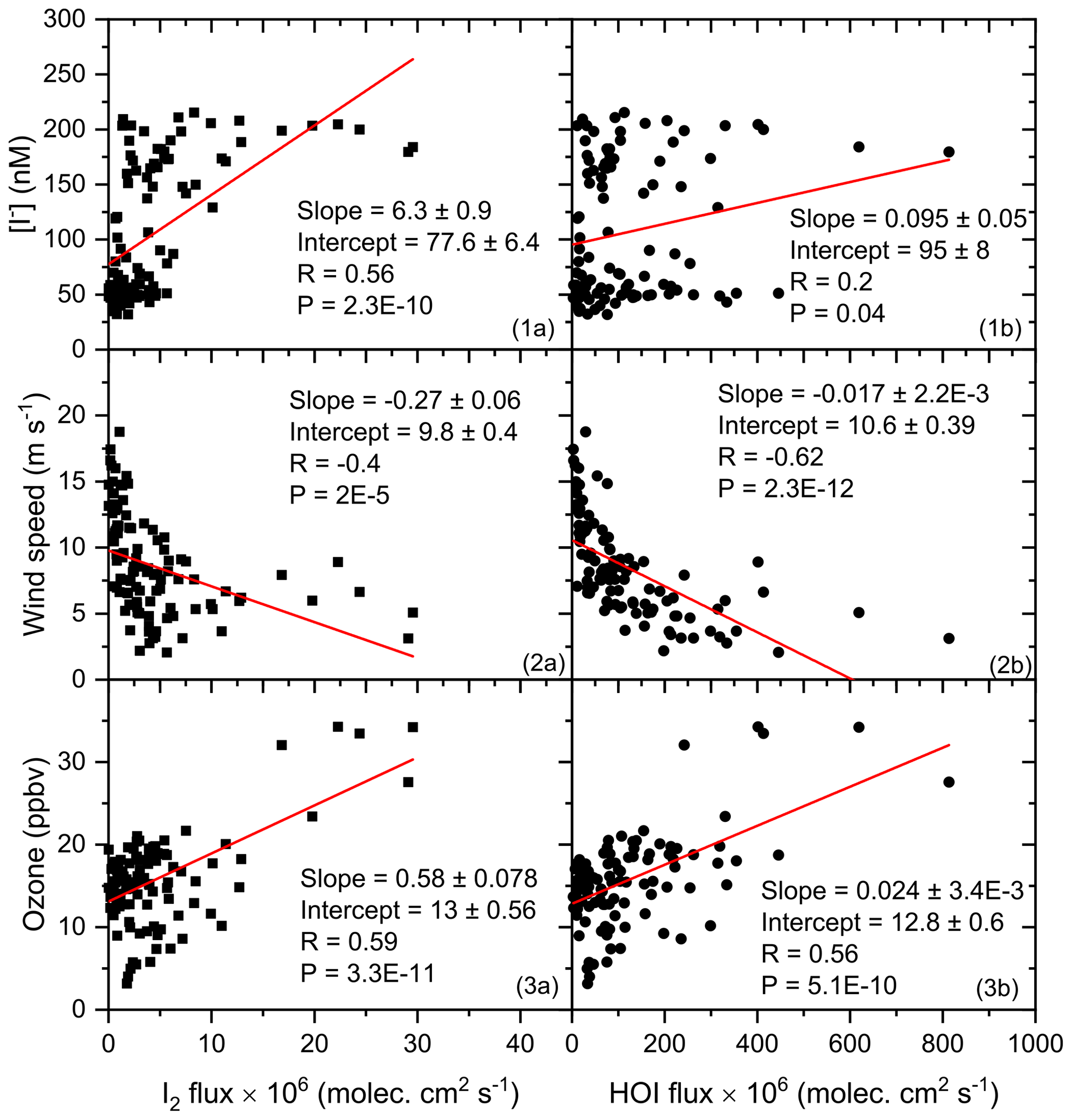
Figure 7Linear fit of daily average sea surface iodide (SSI) concentration, wind speed, and ozone mixing ratio (y axis) against the calculated I2 and HOI flux (x axis) for the entire campaign. HOI and I2 are calculated with SSI estimated using the modified Chance parameterisation for the Indian Ocean and Southern Ocean in Eq. (2).
In Fig. 7, correlations of iodine fluxes estimated using the measured SSI concentrations (Eq. 2) show that fluxes of HOI correlate positively with tropospheric ozone (R=0.56, P<0.001) and negatively to wind speed (, P<0.001), and I2 fluxes correlate positively with SSI concentration (R=0.56, ) and ozone (R=0.59, P<0.001) and negatively with wind speed (, P<0.001). This indicates that there is a positive correlation of I2 with SSI, the dominant inorganic iodine flux (i.e. HOI does not show a significant correlation with the SSI concentration), although the flux equation includes an iodide term (Eq. 8). We analysed the correlation of daily averaged observed IO during the three campaigns with daily averaged values of oceanic parameters (SST, chl a, salinity, SSI concentration), meteorological parameters (wind speed, ozone), and calculated inorganic iodine fluxes. We divided the combined dataset from three campaigns into two regional subsets for the north (Fig. 8a) and south (Fig. 8b) of the polar front (47∘ S). The correlation for SSI concentrations is included for all seven methods for SSI estimation listed in Sect. 2.3. The fluxes of HOI and I2 obtained using the seven different datasets for SSI are included and listed in Fig. 8 in the same order as the SSI concentration (labelled 1 to 7). IO model output from GEOS-Chem (labelled 8) and CAM-Chem (labelled 9) is included for the correlation analysis, along with chl a data from observations during ISOE-8 and ISOE-9 and a satellite dataset obtained from MODIS Aqua (Oceancolor, NASA-GSFC, 2017).
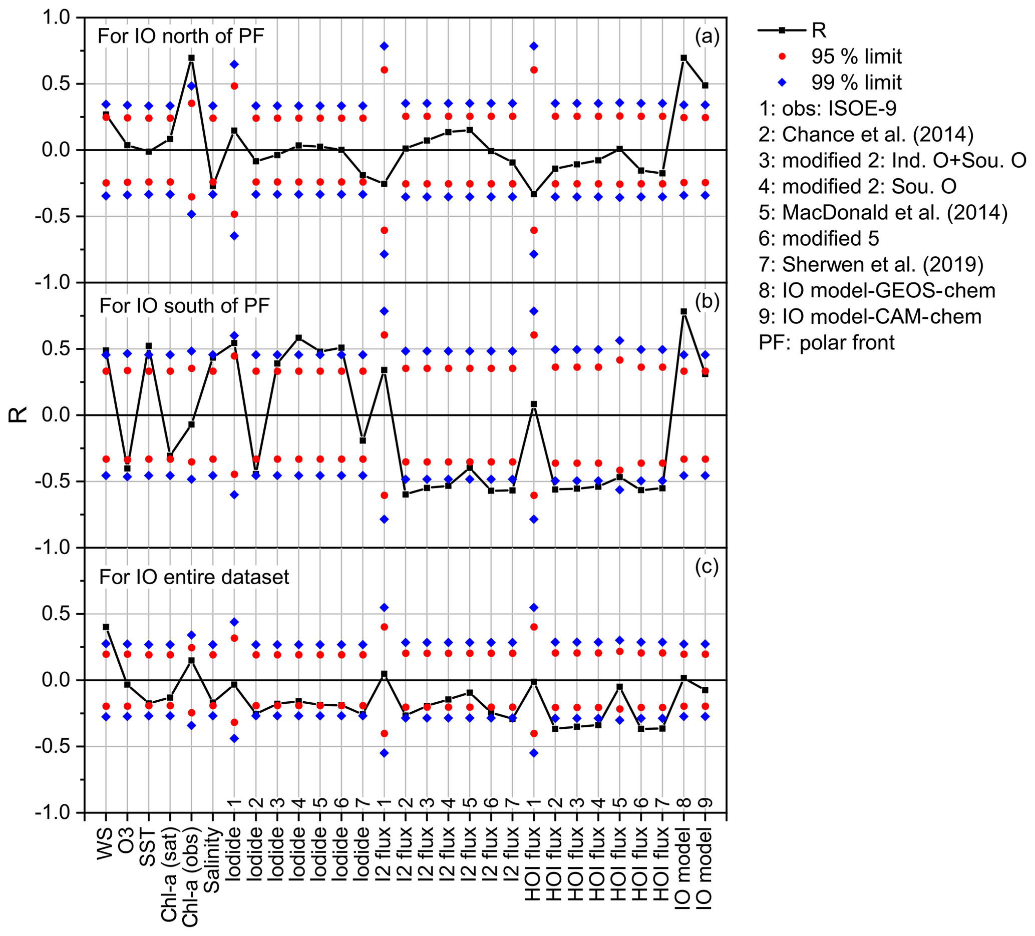
Figure 8The Pearson's correlation coefficient of observed iodine monoxide (IO) with oceanic and atmospheric parameters combined for the ISOE-8, IIOE-2, and ISOE-9 campaigns. Correlations are performed for daily averages of IO and corresponding parameters listed on the x axis. The black squares represent the Pearson's correlation coefficients (R), the diamonds (blue) mark the 99 % confidence limit, and the circles (red) correspond to the 95 % confidence limits in all the panels. Panel (a) includes data from all campaigns to the north of the polar front (PF) (n=72), panel (b) represents combined data for the south of the polar front (n=48), and panel (c) includes the entire dataset from three campaigns (n=120).
For the entire dataset (Fig. 8c), only wind speed shows a statistically significant, positive correlation with observed IO above the 99 % confidence limit (R=0.4, P<0.001, n=115). A similar positive correlation with wind speed was found in the subset of data south of the polar front (Fig. 8b) (R=0.49, P=0.01, n=48), with observations north of the polar front showing a weaker positive correlation (R=0.27, P=0.08, n=67). Mahajan et al. (2012) showed that no correlation existed between IO and wind speed over the eastern Pacific Ocean, contrary to the results in this study. Current estimation methods for iodine emissions have a negative dependence on wind speed (Eqs. 7 and 8). A positive correlation of IO with wind speed could suggest that increased vertical mixing enables the emission of HOI, I2, and/or other iodine gases, thus enhancing IO production in the MBL. However, the interfacial model still overpredicts IO concentrations at low wind speeds due to overprediction of HOI and I2 emissions (MacDonald et al., 2014). The apparently contradictory results from different studies call for more observations of IO in the MBL over a range of wind speeds.
Salinity and SST show a weak negative correlation with atmospheric IO for the entire dataset and for the north of the polar front region. This indicates that even if the physical parameters are significant for the initial parameterisation for SSI and inorganic flux estimation, there is no direct and significant correlation of these parameters with atmospheric IO. However, south of the polar front, SST correlates positively above the 99 % limit (R=0.52, P=0.01, n=48) and salinity correlates positively above the 95 % limit (R=0.44, P=0.03, n=48). Ozone correlates negatively with IO above the 95 % limit (, P=0.046, n=47), which could indicate catalytic destruction of tropospheric ozone through atmospheric iodine cycling in the south of the polar front. This highlights the fact that although these physical parameters may be required for iodine fluxes, IO levels may only be weakly related to them.
The calculated SSI concentrations and the HOI and I2 fluxes calculated using these SSIs all show a significant negative correlation with the observed IO concentrations above the 95 % confidence limit for the entire dataset (except for the HOI flux estimated from the MacDonald et al., 2014, parameterisation, which shows no significant correlation). The positive correlation of the observed IO with wind speed is a potential driver for the negative correlation of observed IO with the calculated HOI and I2 fluxes, which decrease with wind speed.
Measured iodide levels (labelled 4) and the I2 and HOI fluxes calculated from them (also labelled 4) show no correlation with the observed IO levels across the entire dataset, although iodide shows a significant positive correlation (R=0.55, P=0.04, n=32) for IO measured south of the polar front. Mahajan et al. (2019a) pointed out that SST negatively correlated with IO for the ISOE-8 campaign, contradicting the previous results for observations in the Pacific Ocean (Großmann et al., 2013; Mahajan et al., 2012). Here, SST shows a significant positive correlation with observed IO (R=0.52, P=0.006, n=48) south of the polar front above the 99 % confidence limit, but there is no correlation north of the polar front and only a weak negative correlation using the combined dataset from the three campaigns (, P=0.13, n=119).
Despite the above-mentioned point regarding the increase in observed IO levels in regions of elevated chl a, there is only a weak and negative correlation of IO with chl a (from both observations and satellite data) south of the polar front. However, there is a strong positive relationship north of the polar front (R=0.696, , n=29). In fact, for the region north of the polar front, chl a shows a significant positive correlation with observed IO above the 99 % confidence limit (P<0.001). The GEOS-Chem and CAM-Chem output also shows a significant positive correlation (Fig. 8), which may result from the dependency of organic iodine species on oceanic chl a in both GEOS-Chem and CAM-Chem. Figure 8 shows a large difference in correlation values for chl a data obtained from observations and a satellite (MODIS Aqua, NASA, GSFC; https://oceancolor.gsfc.nasa.gov, last access: 12 May 2019; extracted for the same locations as the in situ data). In situ, observed chl a showed an improved correlation with IO compared to that with satellite chl a. Figure 9 shows linear fits for chl a from in situ observations and the satellite against IO for the entire dataset and the subset for north of the polar front. For the entire dataset, the correlation of chl a with IO from both observations and satellite data is not significant. Chl a from in situ observations positively correlates with IO (R=0.15, P=0.32), while chl a from satellite data correlates negatively (, P=0.26). Correlations of chl a with IO improve north of the polar front for chl a from observations (R=0.696, P=0.0002), but chl a from satellite data shows a statistically insignificant correlation with IO (R=0.08, P=0.57). The discrepancies in chl a from observations and satellite data will make it difficult to identify links between the organic parameter and atmospheric IO and expand this to a global scale. It should be noted that one study in the Pacific has shown that the contribution of combined biogenic iodocarbon fluxes to IO does not explain the observed IO (Hepach et al., 2016).

Figure 9Linear fit of daily averaged field observations of chlorophyll a (red circles) and chlorophyll a satellite data (blue circles) (y axis) against observed iodine monoxide (IO) (x axis) from the ISOE-8, IIOE-2, and ISOE-9 campaigns. The top panels include chlorophyll a for the entire dataset; the bottom panels include data to the north of the polar front.
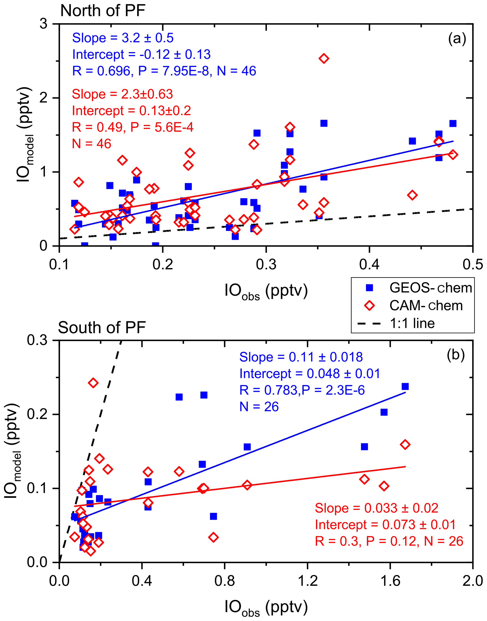
Figure 10Linear fit of daily averages of modelled surface iodine monoxide (IO) output (y axis) from GEOS-Chem (filled blue squares) and CAM-Chem (unfilled red diamonds) against observed IO (x axis) for the ISOE-8, IIOE-2, and ISOE-9 campaigns. Panel (a) includes linear fits of both GEOS-Chem and CAM-Chem for IO detected to the north of the polar front, and panel (b) shows the same for the region south of the polar front. Two data points in (a) at 41 and 43∘ S are removed due to large differences between observations and modelled values.
Despite the observed negative relationship of IO with wind speed noted above, note that the GEOS-Chem IO model output (which is dependent on the calculated HOI and I2 fluxes) shows a significant positive correlation with observed IO above the 99 % confidence limit for data south (R=0.78, , n=48) and north (R=0.69, , n=68) of the polar front, although there is no correlation across the entire dataset. Note that the model underestimates IO values by 1 pptv south of the polar front and generally overestimates IO by ∼1.5 pptv north of the polar front (Fig. 4). A linear fit for observed IO against modelled IO for north and south of the polar front (Fig. 10) shows a significant positive correlation of GEOS-Chem output with observed IO but with very different slopes north of the polar front (where the models overestimate IO) and south of the polar front (where the models underestimate IO). Hence, even though the correlations are good in the individual regions, the model does not accurately reproduce the observed absolute concentrations.
In this study, region-specific parameterisation tools were devised for sea surface iodide (SSI) estimation following previous SSI estimation methods from Chance et al. (2014) and MacDonald et al. (2014). New observations of SSI from ISOE-9, SK-333, and BoBBLE (Indian and the Southern Ocean) were used to create region-specific SSI parameterisations. An average difference of up to 40 % in SSI concentration was observed among the existing parameterisations (Eqs. 1, 4, and 6), and the difference was 21 % for the region-specific ones (Eqs. 2, 3, and 5). Comparison of estimated SSI concentrations from various parameterisations with observed SSI and sensitivity to seasonal salinity changes showed that the modified Chance parameterisation (Eq. 2) was most suitable relative to the SST-based parameterisation (Eq. 5) for SSI estimation in the Indian Ocean and Southern Ocean region. Since the existing global parameterisation schemes (Eqs. 1 and 3) fail to match measured SSI in this region, there is a need to conduct more observations of SSI in the Indian Ocean and Southern Ocean region to fully understand and estimate the impact of seasonally varying, region-specific parameters (like salinity, reversing winds patterns) influencing the seawater iodide concentration in this region. Alternatively, a region-specific parameterisation scheme may be included in the global models for better representation of seawater iodine chemistry in the Indian and Southern Ocean region. Modelled estimates from Sherwen et al. (2019) also captured SSI well, although some high concentrations in the northern Indian Ocean region were not captured. SSI estimation from SST alone underpredicts SSI for the Indian Ocean and is therefore not considered to be suitable for SSI estimation in the Indian Ocean region. Although improving SSI concentration in models for the Indian Ocean and Southern Ocean region may improve the estimation of seawater iodine chemistry, it does not translate to estimating the atmospheric iodine chemistry in this region. An accurate estimation of inorganic iodine fluxes (HOI and I2) is hence necessary to explain observed levels of IO in the remote open-ocean marine boundary layer. However, these first concomitant observations of SSI and IO show that the inorganic fluxes estimated in this study fail to explain detected IO levels for the entire dataset. No significant correlation was seen between the SSI from different parameterisation techniques or estimated inorganic iodine fluxes with observed IO levels. Fluxes estimated using iodide from different parameterisation and measured iodide did not show large variation in values and followed a similar latitudinal trend. This is indicative of the inorganic iodine flux parameterisation not being highly sensitive to the SSI parameterisation. Predicted inorganic iodine fluxes did not explain iodine chemistry, as indicated by IO levels, in the atmosphere above the Indian and Southern Ocean (Indian Ocean sector). Chl a shows a positive correlation with IO for the north of the polar front region, suggesting that biologically emitted species could also play a role in addition to ozone- and iodide-derived inorganic emissions of HOI and I2. Finally, model predictions of IO underestimate IO levels for the Southern Ocean region but overestimate IO in the Indian Ocean. Models greatly underestimate IO in regions with a higher chl a concentration, which could be indicative of organic species playing a role (close to the Kerguelen Islands; refer to Sect. 3.4.2). This study suggests that the fluxes of iodine in the MBL are more complex than considered at present and further studies are necessary in order to parameterise accurate inorganic and organic fluxes that can be used in models. Using seawater iodide measurements and calculations from different parameterisations did not alter the inorganic iodide flux estimate greatly. Direct observations of HOI and I2, alongside volatile organic iodine measurements in the MBL, are necessary in order to reduce the uncertainty in the impacts of iodine chemistry.
All the datasets used in this study are available from Mendeley public data repository at https://doi.org/10.17632/rrn8vpv8mj.1 (Inamdar et al., 2020). Supporting datasets are appropriately cited and linked in the above repository page.
The supplement related to this article is available online at: https://doi.org/10.5194/acp-20-12093-2020-supplement.
ASM conceptualised the research plan and methodology. SI did the data curation, analysis, and writing of the original draft. LT and RC did the iodide measurements and provided unpublished iodide data from ISOE-9, SK-333, and BoBBLE. PS and RCo provided salinity data for ISOE-9. SCT and AUK provided chl a data for ISOE-9. AKS and PVB provided chl a data for SK-333. AS and RR provided chl a data from BoBBLE. CC and ASL did the CAM-Chem model run for ISOE-9 and IIOE-2. TS did the GEOS-Chem model run for ISOE-9, IIOE-2, and ISOE-8.
The authors declare that they have no conflict of interest.
The authors thank the Ministry of Earth Sciences for funding the expeditions and IITM for providing a research fellowship to Swaleha Inamdar. We would particularly like to thank the ISOE and IIOE-2 teams for their tireless contribution to manually recording and compiling atmospheric and oceanic observations during the expedition. We express gratitude to the officers, crew, and scientists on board RV S.A. Agulhas and RV Sagar Kanya for their support.
Lucy J. Carpenter, Liselotte Tinel, Rosie Chance, and Tomás Sherwen received funding from the UK NERC through the grant “Iodide in the ocean: distribution and impact on iodine flux and ozone loss” (grant no. NE/N009983/1).
This paper was edited by Andreas Engel and reviewed by Theodore Koenig and two anonymous referees.
Alicke, B., Hebestreit, K., Stutz, J., and Platt, U.: Iodine oxide in the marine boundary layer, Nature, 397, 572–573, https://doi.org/10.1038/17508, 1999.
Allan, B., McFiggans, G., Plane, J. M. C., and Coe, H.: Observations of iodine monoxide in the remote marine boundary layer, J. Geophys., 105, 14363–14369, 2000.
Atkinson, H. M., Huang, R.-J., Chance, R., Roscoe, H. K., Hughes, C., Davison, B., Schönhardt, A., Mahajan, A. S., Saiz-Lopez, A., Hoffmann, T., and Liss, P. S.: Iodine emissions from the sea ice of the Weddell Sea, Atmos. Chem. Phys., 12, 11229–11244, https://doi.org/10.5194/acp-12-11229-2012, 2012.
Bogumil, K., Orphal, J., Homann, T., Voigt, S., Spietz, P., Fleischmann, O. C., Vogel, A., Hartmann, M., Kromminga, H., Bovensmann, H., Frerick, J., and Burrows, J. P.: Measurements of molecular absorption spectra with the SCIAMACHY pre-flight model: Instrument characterization and reference data for atmospheric remote-sensing in the 230–2380 nm region, J. Photochem. Photobiol. A Chem., 157, 167–184, https://doi.org/10.1016/S1010-6030(03)00062-5, 2003.
Campos, M. L. A. M.: New approach to evaluating dissolved iodine speciation in natural waters using cathodic stripping voltammetry and a storage study for preserving iodine species, Mar. Chem., 57, 107–117, https://doi.org/10.1016/S0304-4203(96)00093-X, 1997.
Carpenter, L. J.: Iodine in the marine boundary layer, Chem. Rev., 103, 4953–4962, https://doi.org/10.1021/Cr0206465, 2003.
Carpenter, L. J., MacDonald, S. M., Shaw, M. D., Kumar, R., Saunders, R. W., Parthipan, R., Wilson, J. and Plane, J. M. C.: Atmospheric iodine levels influenced by sea surface emissions of inorganic iodine, Nat. Geosci., 6, 108–111, https://doi.org/10.1038/ngeo1687, 2013.
Chameides, W. L. and Davis, D. D.: Iodine: Its possible role in tropospheric photochemistry, J. Geophys. Res., 85, 7383–7398, https://doi.org/10.1029/JC085iC12p07383, 1980.
Chance, K. V. and Spurr, R. J. D.: Ring effect studies: Rayleigh scattering, including molecular parameters for rotational Raman scattering, and the Fraunhofer spectrum, Appl. Opt., 36, 5224–5230, https://doi.org/10.1364/AO.36.005224, 1997.
Chance, R., Baker, A. R., Carpenter, L., and Jickells, T. D.: The distribution of iodide at the sea surface, Environ. Sci. Process. Impacts, 16, 1841–1859, https://doi.org/10.1039/C4EM00139G, 2014.
Chance, R., Tinel, L., Sherwen, T., Baker, A., Bell, T., Brindle, J., Campos, M. L. A. M., Croot, P., Ducklow, H., He, P., Hoogakker, B., Hopkins, F. E., Hughes, C., Jickells, T., Loades, D., Macaya, D. A., Mahajan, A. S., Malin, G., Phillips, D. P., Sinha, A. K., Sarkar, A., Roberts, I. J., Roy, R., Song, X., Winklebauer, H. A., Wuttig, K., Yang, M., Zhou, P., and Carpenter, L. J.: Global sea-surface iodide observations, 1967–2018, Nat. Sci. Data, 6, 286, https://doi.org/10.1038/s41597-019-0288-y, 2019.
Chance, R., Tinel, L., Sarkar, A., Sinha, A. K., Mahajan, A. S., Chacko, R., Sabu, P., Roy, R., Jickells, T. D., Stevens, D. P., Wadley, M., and Carpenter, L. J.: Surface Inorganic Iodine Speciation in the Indian and Southern Oceans From 12∘ N to 70∘ S, Front. Mar. Sci., 7, 621, https://doi.org/10.3389/fmars.2020.00621, 2020.
Chang, W., Heikes, B. G., and Lee, M.: Ozone deposition to the sea surface: chemical enhancement and wind speed dependence, Atmos. Environ., 38, 1053–1059, https://doi.org/10.1016/j.atmosenv.2003.10.050, 2004.
D'Addezio, J. M., Subrahmanyam, B., Nyadjro, E. S., and Murty, V. S. N.: Seasonal Variability of Salinity and Salt Transport in the Northern Indian Ocean, J. Phys. Oceanogr., 45, 1947–1966, https://doi.org/10.1175/JPO-D-14-0210.1, 2015.
Danckaert, T., Fayt, C., and Van Roozendael, M.: QDOAS 3.2., available at: http://uv-vis.aeronomie.be/software/QDOAS/QDOAS_manual.pdf, last access: 7 October 2020, 2017.
Davis, D., Crawford, J., Liu, S., McKeen, S., Bandy, A., Thornton, D., Rowland, F. S., and Blake, D.: Potential impact of iodine on tropospheric levels of ozone and other critical oxidants, J. Geophys. Res.-Atmos., 101, 2135–2147, 1996.
Dinesh Kumar, P. K., Paul, Y. S., Muraleedharan, K. R., Murty, V. S. N., and Preenu, P. N.: Comparison of long-term variability of Sea Surface Temperature in the Arabian Sea and Bay of Bengal, Reg. Stud. Mar. Sci., 3, 67–75, https://doi.org/10.1016/j.rsma.2015.05.004, 2016.
Farrenkopf, A. M. and Luther, G. W.: Iodine chemistry reflects productivity and denitrification in the Arabian Sea?: evidence for flux of dissolved species from sediments of western India into the OMZ, Deep Sea Res.-Pt II, 49, 2303–2318, 2002.
Frieß, U., Wagner, T., Pundt, I., Pfeilsticker, K., Platt, U., and Friefi, U.: Spectroscopic Measurements of Tropospheric Iodine Oxide at Neumayer Station, Antarctica, Geophys. Res. Lett., 28, 1941–1944, 2001.
Gálvez, Ó., Teresa Baeza-Romero, M., Sanz, M., and Pacios, L. F.: A theoretical study on the reaction of ozone with aqueous iodide, Phys. Chem. Chem. Phys., 18, 7651–7660, https://doi.org/10.1039/c5cp06440f, 2016.
Ganzeveld, L., Helmig, D., Fairall, C. W., Hare, J., and Pozzer, A.: Atmosphere-ocean ozone exchange: A global modeling study of biogeochemical, atmospheric, and waterside turbulence dependencies, Global Biogeochem. Cy., 23, 1–16, https://doi.org/10.1029/2008GB003301, 2009.
Garland, J. A., Elzerman, A. W., Penkett, S. A., and Penket, S. A.: The Mechanism for Dry Deposition of Ozone to Seawater Surfaces, J. Geophys. Res., 85, 7488–7492, 1980.
Großmann, K., Frieß, U., Peters, E., Wittrock, F., Lampel, J., Yilmaz, S., Tschritter, J., Sommariva, R., von Glasow, R., Quack, B., Krüger, K., Pfeilsticker, K., and Platt, U.: Iodine monoxide in the Western Pacific marine boundary layer, Atmos. Chem. Phys., 13, 3363–3378, https://doi.org/10.5194/acp-13-3363-2013, 2013.
Hepach, H., Quack, B., Tegtmeier, S., Engel, A., Bracher, A., Fuhlbrügge, S., Galgani, L., Atlas, E. L., Lampel, J., Frieß, U., and Krüger, K.: Biogenic halocarbons from the Peruvian upwelling region as tropospheric halogen source, Atmos. Chem. Phys., 16, 12219–12237, https://doi.org/10.5194/acp-16-12219-2016, 2016.
Hönninger, G., von Friedeburg, C., and Platt, U.: Multi axis differential optical absorption spectroscopy (MAX-DOAS), Atmos. Chem. Phys., 4, 231–254, https://doi.org/10.5194/acp-4-231-2004, 2004.
Hossaini, R., Chipperfield, M. P., Saiz-Lopez, A., Fernandez, R., Monks, S., Feng, W., Brauer, P., and Von Glasow, R.: A global model of tropospheric chlorine chemistry: Organic versus inorganic sources and impact on methane oxidation, J. Geophys. Res., 121, 14271–14297, https://doi.org/10.1002/2016JD025756, 2016.
Huang, R. J., Seitz, K., Neary, T., O'Dowd, C. D., Platt, U., and Hoffmann, T.: Observations of high concentrations of I2 and IO in coastal air supporting iodine-oxide driven coastal new particle formation, Geophys. Res. Lett., 37, 1–5, https://doi.org/10.1029/2009GL041467, 2010.
Inamdar, S., Tinel, L., Chance, R., Carpenter, L., Sabu, P., Chacko, R., Tripathy, S., Kerkar, U. A., Sinha, A., Bhaskar, P., Sarkar, A., Roy, R., Sherwen, T., Cuevas, C. A., Saiz-Lopez, A., Ram, K., and Mahajan, A.: Dataset of Estimation of reactive inorganic iodine fluxes in the Indian and Southern Ocean marine boundary layer, Mendeley Data, V1, https://doi.org/10.17632/rrn8vpv8mj.1, 2020.
Jenkin, M. E., Cox, R. A., Candeland, D. E., and Division, M. S.: Photochemical aspects of tropospheric iodine behaviour, J. Atmos. Chem., 2, 359–375, https://doi.org/10.1007/BF00130748, 1985.
Koenig, T. K., Baidar, S., Campuzano-Jost, P., Cuevas, C. A., Dix, B., Fernandez, R. P., Guo, H., Hall, S. R., Kinnison, D., Nault, B. A., Ullmann, K., Jimenez, J. L., Saiz-Lopez, A., and Volkamer, R.: Quantitative detection of iodine in the stratosphere, P. Natl. Acad. Sci. USA, 15, 201916828, https://doi.org/10.1073/pnas.1916828117, 2020.
Lawler, M. J., Mahajan, A. S., Saiz-Lopez, A., and Saltzman, E. S.: Observations of I2 at a remote marine site, Atmos. Chem. Phys., 14, 2669–2678, https://doi.org/10.5194/acp-14-2669-2014, 2014.
Luther, G. W., Swartz, C. B., and Ullman, W. J.: Direct determination of iodide in seawater by cathodic stripping square wave voltammetry, Anal. Chem., 60, 1721–1724, https://doi.org/10.1021/ac00168a017, 1988.
MacDonald, S. M., Gómez Martín, J. C., Chance, R., Warriner, S., Saiz-Lopez, A., Carpenter, L. J., and Plane, J. M. C.: A laboratory characterisation of inorganic iodine emissions from the sea surface: dependence on oceanic variables and parameterisation for global modelling, Atmos. Chem. Phys., 14, 5841–5852, https://doi.org/10.5194/acp-14-5841-2014, 2014.
Mahajan, A. S., Oetjen, H., Saiz-Lopez, A., Lee, J. D., McFiggans, G. B., and Plane, J. M. C.: Reactive iodine species in a semi-polluted environment, Geophys. Res. Lett., 36, L16803, https://doi.org/10.1029/2009GL038018, 2009.
Mahajan, A. S., Shaw, M., Oetjen, H., Hornsby, K. E., Carpenter, L. J., Kaleschke, L., Tian-Kunze, X., Lee, J. D., Moller, S. J., Edwards, P. M., Commane, R., Ingham, T., Heard, D. E., and Plane, J. M. C.: Evidence of reactive iodine chemistry in the Arctic boundary layer, J. Geophys. Res., 115, D20303, https://doi.org/10.1029/2009JD013665, 2010a.
Mahajan, A. S., Plane, J. M. C., Oetjen, H., Mendes, L., Saunders, R. W., Saiz-Lopez, A., Jones, C. E., Carpenter, L. J., and McFiggans, G. B.: Measurement and modelling of tropospheric reactive halogen species over the tropical Atlantic Ocean, Atmos. Chem. Phys., 10, 4611–4624, https://doi.org/10.5194/acp-10-4611-2010, 2010b.
Mahajan, A. S., Gómez Martín, J. C., Hay, T. D., Royer, S.-J., Yvon-Lewis, S., Liu, Y., Hu, L., Prados-Roman, C., Ordóñez, C., Plane, J. M. C., and Saiz-Lopez, A.: Latitudinal distribution of reactive iodine in the Eastern Pacific and its link to open ocean sources, Atmos. Chem. Phys., 12, 11609–11617, https://doi.org/10.5194/acp-12-11609-2012, 2012.
Mahajan, A. S., Tinel, L., Hulswar, S., Cuevas, C. A., Wang, S., Ghude, S., Naik, R. K., Mishra, R. K., Sabu, P., Sarkar, A., Anilkumar, N. and Saiz-Lopez, A.: Observations of iodine oxide in the Indian Ocean Marine Boundary Layer: a transect from the tropics to the high latitudes, Atmos. Environ., 1, 100016, https://doi.org/10.1016/j.aeaoa.2019.100016, 2019a.
Mahajan, A. S., Tinel, L., Sarkar, A., Chance, R., Carpenter, L. J., Hulswar, S., Mali, P., Prakash, S. and Vinayachandran, P. N.: Understanding Iodine Chemistry over the Northern and Equatorial Indian Ocean, J. Geophys. Res. Atmos., 124, 8104–8118, https://doi.org/10.1029/2018JD029063, 2019b.
McFiggans, G. B.: Marine aerosols and iodine emissions, Nature, 433, 7026, https://doi.org/10.1038/nature03372, 2005.
Monterey, G. and Levitus, S.: Seasonal Variability of Mixed Layer Depth for the World Ocean, U.S. Government Printing Office, Washington, D.C., 102 pp., 1997.
Moreno, C. and Baeza-Romero, M. T.: A kinetic model for ozone uptake by solutions and aqueous particles containing I- and Br-, including seawater and sea-salt aerosol, Phys. Chem. Chem. Phys., 21, 19835–19856, https://doi.org/10.1039/C9CP03430G, 2019.
O'Dowd, C. D., Jimenez, J. L., Bahreini, R., Flagan, R. C., Seinfeld, J. H., Hämeri, K., Pirjola, L., Kulmala, M., Gerard Jennings, S., Hoffmann, T., Hameri, K. and Jennings, S. G.: Marine aerosol formation from biogenic iodine emissions, Nature, 417, 632–636, 2002.
Ordóñez, C., Lamarque, J.-F., Tilmes, S., Kinnison, D. E., Atlas, E. L., Blake, D. R., Sousa Santos, G., Brasseur, G., and Saiz-Lopez, A.: Bromine and iodine chemistry in a global chemistry-climate model: description and evaluation of very short-lived oceanic sources, Atmos. Chem. Phys., 12, 1423–1447, https://doi.org/10.5194/acp-12-1423-2012, 2012.
Platt, U. and Stutz, J.: Differential Absorption Spectroscopy, in Differential Optical Absorption Spectroscopy, Springer, Berlin, Heidelberg, 135–174, 2008.
Pope, R. M. and Fry, E. S.: Absorption spectrum (380–700 nm) ofpure water, II. Integrating cavity measurements, Appl. Opt., 36, 8710–8723, 1997.
Prados-Roman, C., Cuevas, C. A., Hay, T., Fernandez, R. P., Mahajan, A. S., Royer, S.-J., Galí, M., Simó, R., Dachs, J., Großmann, K., Kinnison, D. E., Lamarque, J.-F., and Saiz-Lopez, A.: Iodine oxide in the global marine boundary layer, Atmos. Chem. Phys., 15, 583–593, https://doi.org/10.5194/acp-15-583-2015, 2015.
Rao, R. R. and Sivakumar, R.: Seasonal variability of sea surface salinity and salt budget of the mixed layer of the north Indian Ocean, J. Geophys. Res., 108, 3009, https://doi.org/10.1029/2001JC000907, 2003.
Read, K. A., Mahajan, A. S., Carpenter, L. J., Evans, M. J., Faria, B. V. E., Heard, D. E., Hopkins, J. R., Lee, J. D., Moller, S. J., Lewis, A. C., Mendes, L. M., McQuaid, J. B., Oetjen, H., Saiz-Lopez, A., Pilling, M. J. and Plane, J. M. C.: Extensive halogen-mediated ozone destruction over the tropical Atlantic Ocean, Nature, 453, 1232–1235, https://doi.org/10.1038/nature07035, 2008.
Rolph, G., Stein, A., and Stunder, B.: Real-time Environmental Applications and Display sYstem: READY, Environ. Model. Softw., 95, 210–228, https://doi.org/10.1016/j.envsoft.2017.06.025, 2017.
Rothman, L. S., Gordon, I. E., Babikov, Y., Barbe, A., Chris Benner, D., Bernath, P. F., Birk, M., Bizzocchi, L., Boudon, V., Brown, L. R., Campargue, A., Chance, K., Cohen, E. A., Coudert, L. H., Devi, V. M., Drouin, B. J., Fayt, A., Flaud, J. M., Gamache, R. R., Harrison, J. J., Hartmann, J. M., Hill, C., Hodges, J. T., Jacquemart, D., Jolly, A., Lamouroux, J., Le Roy, R. J., Li, G., Long, D. A., Lyulin, O. M., Mackie, C. J., Massie, S. T., Mikhailenko, S., Müller, H. S. P., Naumenko, O. V., Nikitin, A. V., Orphal, J., Perevalov, V., Perrin, A., Polovtseva, E. R., Richard, C., Smith, M. A. H., Starikova, E., Sung, K., Tashkun, S., Tennyson, J., Toon, G. C., Tyuterev, V. G., and Wagner, G.: The HITRAN2012 molecular spectroscopic database, J. Quant. Spectrosc. Ra., 130, 4–50, https://doi.org/10.1016/j.jqsrt.2013.07.002, 2013.
Saiz-Lopez, A., Shillito, J. A., Coe, H., and Plane, J. M. C.: Measurements and modelling of I2, IO, OIO, BrO and NO3 in the mid-latitude marine boundary layer, Atmos. Chem. Phys., 6, 1513–1528, https://doi.org/10.5194/acp-6-1513-2006, 2006.
Saiz-Lopez, A. and Fernandez, R. P.: On the formation of tropical rings of atomic halogens: Causes and implications, Geophys. Res. Lett., 43, 1–8, https://doi.org/10.1002/2015GL067608, 2016.
Saiz-Lopez, A. and Plane, J. M. C.: Novel iodine chemistry in the marine boundary layer, Geophys. Res. Lett., 31, L04112, https://doi.org/10.1029/2003GL019215, 2004.
Saiz-Lopez, A., Plane, J. M. C., McFiggans, G., Williams, P. I., Ball, S. M., Bitter, M., Jones, R. L., Hongwei, C., and Hoffmann, T.: Modelling molecular iodine emissions in a coastal marine environment: the link to new particle formation, Atmos. Chem. Phys., 6, 883–895, https://doi.org/10.5194/acp-6-883-2006, 2006.
Saiz-Lopez, A., Plane, J. M. C., Baker, A. R., Carpenter, L. J., von Glasow, R., Martín, J. C. G., McFiggans, G. B., Saunders, R. W., and Gómez Martín, J. C.: Atmospheric Chemistry of Iodine, Chem. Rev., 112, 1773–1804, https://doi.org/10.1021/cr200029u, 2012.
Saiz-Lopez, A., Fernandez, R. P., Ordóñez, C., Kinnison, D. E., Gómez Martín, J. C., Lamarque, J.-F., and Tilmes, S.: Iodine chemistry in the troposphere and its effect on ozone, Atmos. Chem. Phys., 14, 13119–13143, https://doi.org/10.5194/acp-14-13119-2014, 2014.
Shenoi, S. S. C.: Differences in heat budgets of the near-surface Arabian Sea and Bay of Bengal: Implications for the summer monsoon, J. Geophys. Res., 107, 3052, https://doi.org/10.1029/2000JC000679, 2002.
Sherwen, T., Schmidt, J. A., Evans, M. J., Carpenter, L. J., Großmann, K., Eastham, S. D., Jacob, D. J., Dix, B., Koenig, T. K., Sinreich, R., Ortega, I., Volkamer, R., Saiz-Lopez, A., Prados-Roman, C., Mahajan, A. S., and Ordóñez, C.: Global impacts of tropospheric halogens (Cl, Br, I) on oxidants and composition in GEOS-Chem, Atmos. Chem. Phys., 16, 12239–12271, https://doi.org/10.5194/acp-16-12239-2016, 2016a.
Sherwen, T., Evans, M. J., Spracklen, D. V., Carpenter, L. J., Chance, R., Baker, A. R., Schmidt, J. A., and Breider, T. J.: Global modeling of tropospheric iodine aerosol, Geophys. Res. Lett., 43, 10012–10019, https://doi.org/10.1002/2016GL070062, 2016b.
Sherwen, T., Evans, M. J., Carpenter, L. J., Andrews, S. J., Lidster, R. T., Dix, B., Koenig, T. K., Sinreich, R., Ortega, I., Volkamer, R., Saiz-Lopez, A., Prados-Roman, C., Mahajan, A. S., and Ordóñez, C.: Iodine's impact on tropospheric oxidants: a global model study in GEOS-Chem, Atmos. Chem. Phys., 16, 1161–1186, https://doi.org/10.5194/acp-16-1161-2016, 2016c.
Sherwen, T., Evans, M. J., Sommariva, R., Hollis, L. D. J., Ball, S. M., Monks, P. S., Reed, C., Carpenter, L. J., Lee, J. D., Forster, G., Bandy, B., Reeves, C. E., and Bloss, W. J.: Effects of halogens on European air-quality, Faraday Discuss., 200, 75–100, https://doi.org/10.1039/C7FD00026J, 2017.
Sherwen, T., Chance, R. J., Tinel, L., Ellis, D., Evans, M. J., and Carpenter, L. J.: A machine-learning-based global sea-surface iodide distribution, Earth Syst. Sci. Data, 11, 1239–1262, https://doi.org/10.5194/essd-11-1239-2019, 2019.
Simpson, W. R., Brown, S. S., Saiz-Lopez, A., Thornton, J. A., and Glasow, R.: Tropospheric Halogen Chemistry: Sources, Cycling, and Impacts, Chem. Rev., 115, 4035–4062, https://doi.org/10.1021/cr5006638, 2015.
Sinreich, R., Coburn, S., Dix, B., and Volkamer, R.: Ship-based detection of glyoxal over the remote tropical Pacific Ocean, Atmos. Chem. Phys., 10, 11359–11371, https://doi.org/10.5194/acp-10-11359-2010, 2010.
Stein, A. F., Draxler, R. R., Rolph, G. D., Stunder, B. J. B., Cohen, M. D., and Ngan, F.: Noaa's hysplit atmospheric transport and dispersion modeling system, B. Am. Meteorol. Soc., 96, 2059–2077, https://doi.org/10.1175/BAMS-D-14-00110.1, 2015.
Stone, D., Sherwen, T., Evans, M. J., Vaughan, S., Ingham, T., Whalley, L. K., Edwards, P. M., Read, K. A., Lee, J. D., Moller, S. J., Carpenter, L. J., Lewis, A. C., and Heard, D. E.: Impacts of bromine and iodine chemistry on tropospheric OH and HO2: comparing observations with box and global model perspectives, Atmos. Chem. Phys., 18, 3541–3561, https://doi.org/10.5194/acp-18-3541-2018, 2018.
Thalman, R. and Volkamer, R. A.: Temperature Dependent Absorption Cross-Sections of O2-O2 collision pairs between 340 and 630 nm and at atmospherically relevant pressure, Phys. Chem. Chem. Phys., 15, 15371–15381, https://doi.org/10.1039/C3CP50968K, 2013.
Vandaele, A. C., Hermans, C., Simon, P. C., Carleer, M., Colin, R., Fally, S., Mérienne, M. F., Jenouvrier, A., and Coquart, B.: Measurements of the NO2 absorption cross-section from 42000 cm−1 to 10000 cm−1 (238–1000 nm) at 220 K and 294 K, J. Quant. Spectrosc. Ra., 59, 171–184, https://doi.org/10.1016/S0022-4073(97)00168-4, 1998.
Vogt, R., Sander, R., von Glasow, R., and Crutzen, P. J.: Iodine Chemistry and its Role in Halogen Activation and Ozone Loss in the Marine Boundary Layer: A Model Study, J. Atmos. Chem., 32, 375–395, 1999.
Wagner, T., Dix, B., Friedeburg, C. V., Frieß, U., Sanghavi, S., Sinreich, R., and Platt, U.: MAX-DOAS O4 measurements: A new technique to derive information on atmospheric aerosols – Principles and information content, J. Geophys. Res.-Atmos., 109, 1–19, https://doi.org/10.1029/2004JD004904, 2004.
Wagner, T., Beirle, S., and Deutschmann, T.: Three-dimensional simulation of the Ring effect in observations of scattered sun light using Monte Carlo radiative transfer models, Atmos. Meas. Tech., 2, 113–124, https://doi.org/10.5194/amt-2-113-2009, 2009.