the Creative Commons Attribution 4.0 License.
the Creative Commons Attribution 4.0 License.
 | 22 Oct 2020
Using a coupled large-eddy simulation–aerosol radiation model to investigate urban haze: sensitivity to aerosol loading and meteorological conditions
Jessica Slater
Juha Tonttila
Gordon McFiggans
Paul Connolly
Sami Romakkaniemi
Thomas Kühn
The aerosol–radiation–meteorology feedback loop is the process by which aerosols interact with solar radiation to influence boundary layer meteorology. Through this feedback, aerosols cause cooling of the surface, resulting in reduced buoyant turbulence, enhanced atmospheric stratification and suppressed boundary layer growth. These changes in meteorology result in the accumulation of aerosols in a shallow boundary layer, which can enhance the extent of aerosol–radiation interactions. The feedback effect is thought to be important during periods of high aerosol concentrations, for example, during urban haze. However, direct quantification and isolation of the factors and processes affecting the feedback loop have thus far been limited to observations and low-resolution modelling studies. The coupled large-eddy simulation (LES)–aerosol model, the University of California, Los Angeles large-eddy simulation – Sectional Aerosol Scheme for Large Scale Applications (UCLALES-SALSA), allows for direct interpretation on the sensitivity of boundary layer dynamics to aerosol perturbations. In this work, UCLALES-SALSA has for the first time been explicitly set up to model the urban environment, including addition of an anthropogenic heat flux and treatment of heat storage terms, to examine the sensitivity of meteorology to the newly coupled aerosol–radiation scheme. We find that (a) sensitivity of boundary layer dynamics in the model to initial meteorological conditions is extremely high, (b) simulations with high aerosol loading (220 µg m−3) compared to low aerosol loading (55 µg m−3) cause overall surface cooling and a reduction in sensible heat flux, turbulent kinetic energy and planetary boundary layer height for all 3 d examined, and (c) initial meteorological conditions impact the vertical distribution of aerosols throughout the day.
- Article
(668 KB) - Full-text XML
- BibTeX
- EndNote


Severe air pollution events are a major health issue for megacities worldwide, particularly in nations with large populations and high levels of industrialisation such as India and China. Beijing, situated in the North China Plain, is well known for its air quality issues, where concentrations of PM2.5 (particulate matter with an aerodynamic diameter <2.5 µm) frequently exceed the World Health Organisation's recommended hourly exposure limit of 25 µg m−3. Heavy “haze” periods envelop Beijing due to a complex combination of emission sources and unfavourable meteorology. Observations have identified the importance of changing synoptic conditions on the onset of haze episodes, while the longevity and intensity of the episodes are found to be affected by aerosol–radiation interactions (Wang et al., 2019). These interactions feed back on boundary layer meteorology to cause unfavourable conditions such as temperature inversions, increased humidity and decreased wind speed (Dou et al., 2015; Zhang et al., 2015, 2017; Zhong et al., 2019b).
In addition to the unfavourable meteorological conditions, heavy emissions and regional transport of pollutants into Beijing cause high concentrations of urban aerosol particles to accumulate. These particles can either scatter or absorb solar radiation, depending on their composition. Observations predominantly show that aerosol particles cause net cooling at the surface and warming in the upper atmosphere. This consequently alters the thermal profile of the atmosphere, reducing turbulence due to buoyancy. Reduced turbulent mixing suppresses boundary layer development during the day, minimises the vertical mixing of pollutants and increases surface aerosol concentrations. Furthermore, reduction in planetary boundary layer (PBL) height due to the feedback effect also increases water vapour concentrations which can result in enhanced aqueous heterogeneous reactions, thus increasing the rate of secondary aerosol formation. If the aerosol particles are hygroscopic, increased water vapour concentrations will also cause particle growth, resulting in stronger aerosol–radiation interactions. This positive feedback loop between aerosols, radiation and meteorology can lead to sustained periods of stagnation and has been found to enhance pollution events (Fig. 1) (Q. Liu et al., 2018; Luan et al., 2018; Petäjä et al., 2016).
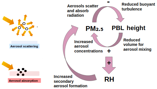
Figure 1Schematic of the positive feedback loop between aerosols, radiation and meteorology thought to enhance pollution episodes in Beijing.
Aerosol composition and size are the main factors impacting an aerosol particle's single scattering albedo, thus impacting the extent by which it will interact with radiation. Most aerosol particles predominately scatter radiation and thus have an overall cooling effect, stabilising the boundary layer and allowing for further accumulation of aerosol particles. However, black carbon (BC), an absorbing aerosol which can contribute up to 10 % of PM in Beijing (Liu et al., 2016), has the potential to have the opposite effect, through warming of the lower atmosphere, which promotes buoyancy and destabilises the boundary layer. However, depending on the vertical distribution of the BC layer, BC can also enhance stratification by causing warming in the upper PBL (Q. Liu et al., 2018; Zhong et al., 2018a; Ding et al., 2016).
Research examining the feedback effect on Beijing haze episodes has thus far relied upon observations or regional modelling studies. Q. Liu et al. (2018), Zhong et al. (2018b), Gao et al. (2015) and Wu et al. (2019) performed model simulations of pollution episodes using the Weather Research and Forecasting model with added chemistry (WRF-Chem) to examine the feedback effect. Their results all confirm that aerosol–radiation interactions, aerosol hygroscopic growth and aqueous heterogeneous reactions are all factors in the suppression of boundary layer development and result in increased surface PM2.5 concentrations during polluted episodes in the North China Plain. Gao et al. (2015) suggest that aerosol–radiation interactions decrease temperature and shortwave (SW) radiation at the surface while increasing them aloft (925 hPa). Examining the feedback from a quantitative perspective, Wu et al. (2019) found that when PM2.5 increased from 50 to 200 µg m−3, maximum average boundary layer height decreased from 700 to 400 m. Furthermore, Zhong et al. (2019a) suggested that threshold PM2.5 concentrations of 75–100 µg m−3 exist in Beijing, above which the feedback effect is increasingly important and leads to aerosol accumulation and exacerbation of pollution episodes.
Observational studies also show a link between aerosol concentrations and boundary layer meteorology. Zou et al. (2017) studied the impact of high aerosol concentrations (PM2.5>75 µg m−3) on Beijing meteorology over a year-long period. Their results demonstrate that the aerosol impact on meteorology was different depending on the season, with particularly large reductions in sensible heat flux (SHF), PBL height and surface SW radiation reported in autumn and winter. Liu et al. (2019) used the same PM2.5 threshold to estimate the impact of high aerosol concentrations on observed meteorological data over a 1-month period where haze episodes occurred every 4–7 d. Comparing high and low aerosol periods, they found that on average surface SW radiation was 36 % lower and daily maximum PBL height was reduced from 1.3 to 0.6 km.
Despite an increase in research in this area, quantification of aerosol perturbations on boundary layer meteorology is still uncertain. In WRF-Chem, results are strongly dependent on the boundary layer scheme or parameterisation employed throughout the simulations, while observations of this effect, although useful, only show links between the phenomena without being able to quantify the processes or separate factors. High-resolution sensitivity studies which allow for direct analysis of boundary layer meteorology are therefore needed to be able to assimilate the major contributions to haze events.
Large-eddy simulations (LESs) can explicitly resolve large, high-energy eddies while parameterising smaller eddies for computational efficiency. This allows for direct investigation of boundary layer meteorology, turbulent fluxes and statistics, while easily controlled conditions allow for insight into the sensitivity of aerosol interactions on PBL dynamics (Q. Liu et al., 2018; Mazoyer et al., 2017). Several studies have used LES models to examine the impact of aerosols on convective boundary layers, cumulus clouds and radiation fogs, primarily in rural or marine environments (Mukherjee et al., 2016; Tonttila et al., 2017; Bellon and Stevens, 2012; Sullivan and Patton, 2011; Andrejczuk et al., 2014). In this work, a novel LES with a coupled sectional aerosol module (the University of California, Los Angeles large-eddy simulation – Sectional Aerosol Scheme for Large Scale Applications; UCLALES-SALSA) has been developed to make it suitable for the urban environment of Beijing. The newly coupled aerosol–radiation scheme has been tested for the first time, in order to examine the feedback effect of aerosol loading on boundary layer dynamics. Model description and details of the setup for an urban environment are outlined in Sect. 2, Sect. 3 describes the experimental setup for cases 1, 2 and 3, Sect. 4 shows results of the simulations, and Sect. 5 discusses the results, including sensitivity of UCLALES-SALSA to meteorological conditions (Sect. 5.1), aerosol loading (Sect. 5.2) and aerosol vertical profiles (Sect. 5.3).
The model used in this work is UCLALES-SALSA. A comprehensive description of the model and its previous uses can be found in the paper by Tonttila et al. (2017). The version used here can be downloaded at https://www.github.com/UCLALES-SALSA (last access: 24 January 2020). A description of the model setup, validation and sensitivity to parameters is given below.
2.1 UCLALES
UCLALES is a large-eddy simulation which has mainly been used in idealised cloud and fog studies. It is based on the Smagorinsky–Lilly subgrid model and solves the Ogura–Phillips anelastic equations with an Asselin filter. Boundary conditions are doubly periodic in the horizontal and fixed in the vertical. Momentum variables are advected with leapfrog time stepping and scalar variables through forward time stepping. In the standard model, a two-moment warm rain microphysical scheme is used, the vertical is spanned by a stretchable grid, and a sponge layer is applied at the domain top to prevent gravity waves being released into the boundary (Stevens et al., 2003, 2005; Tonttila et al., 2017). The surface scheme explicitly calculates SHF and latent heat flux (LHF) at each time step and is based on a coupled soil moisture and surface temperature scheme by Ács et al. (1991) (Eqs. 1, 2 and 3):
where ρ is air density, Cp is specific heat capacity of dry air, Tg and Ta are surface and air temperature, respectively, γ is the psychrometric constant, fh is a dimensionless function related to water volume fraction and takes the value 0.267 in our case. es (Tg) is saturation vapour pressure at surface temperature (Tg) and es is water vapour at 2 m height. rsurf is the surface resistance to bare soil and is related to surface friction velocity (u∗). ra is atmospheric resistance to water vapour and heat and is dependent on atmospheric stability (Ács et al., 1991).
Surface parameters, which vary greatly in different environments, can be varied within the model input and largely affect the heat storage term (ΔQs) (Eq. 3). Here, Ch is volumetric heat capacity (J m−3 K−1), λ is thermal conductivity (W m−1 K−1), ω is angular frequency (s−1) and (K) is the average daily temperature in the 2 cm soil layer. The resulting parameters as well as the overall radiation are utilised in the surface energy balance scheme detailed in (Eq. 4), where Q∗ is net all-wave radiation.
2.2 SALSA
SALSA was developed by Kokkola et al. (2008) and has been coupled with large-eddy simulation models (UCLALES) as well as a climate model (ECHAM) (Kokkola et al., 2018; Tonttila et al., 2017). SALSA bins aerosols according to size, allowing for a variety of aerosol sizes and compositions as well as for aerosols to be either internally or externally mixed (Fig. 2; Kokkola et al., 2008). When SALSA is used in these simulations, aerosol species included are black carbon, sulfate, organic carbon, nitrate and ammonium, with all aerosols assumed to be internally mixed. In terms of aerosol processes, coagulation and water vapour condensation are switched on, while nucleation, aerosol deposition, emissions and semi-volatile condensation are not considered here for simplicity but may be considered in future work.
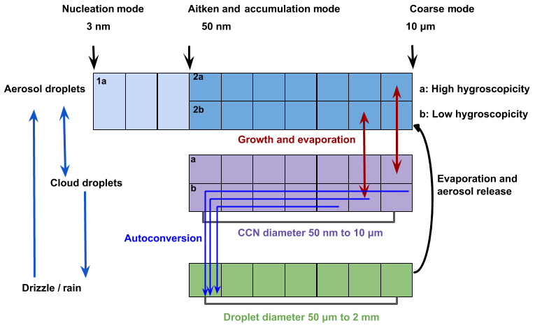
Figure 2Schematic of the size bin layout for SALSA including the internal and external mixing size bins and the cloud and rain droplet bins (Tonttila et al., 2017).
2.3 UCLALES-SALSA
UCLALES-SALSA couples the UCLALES with SALSA and is primarily described in the paper by Tonttila et al. (2017). The version of UCLALES-SALSA here is a fully coupled radiation–dynamical model, whereby the aerosol–radiation interactions in SALSA are fully coupled with the four-stream radiative solver in UCLALES which feeds back on boundary layer turbulence. This is the first time that aerosol–radiation interactions have been dynamically coupled to UCLALES and the work outlined here examines the sensitivity of aerosol loading to these interactions and feedback.
2.3.1 Aerosol–radiation interactions
The solution for radiative transfer in UCLALES is based on the four-stream method integrating over 6 shortwave bands and 12 longwave bands according to Fu and Liou (1993). In this work, the scheme has been adapted to account for the sectional size distribution of the atmospheric aerosol. To this end, we use pre-compiled look-up tables of the aerosol extinction cross section, asymmetry parameter and single scattering albedo, which are given as a function of the size parameter (particle diameter divided by wavelength) and the real and imaginary parts of the refractive index. For a given aerosol constituent, the refractive indices are catalogued at specific wavelengths. Nearest-neighbour interpolation is used to find the values closest to the centres of the wavelength bands used by the radiation solver. Assuming a perfect internal mixture of all aerosol constituents within one aerosol size section, the refractive index in that size section is then calculated as a volume-weighted average of its constituents. This yields the optical thickness, single scattering albedo and phase function parameters weighted by the actual particle size distribution resolved by SALSA, which are then taken to the four-stream integration (Fu and Liou, 1993). The real and imaginary refractive indices for each aerosol component and their use in this simulation are based on Bond and Bergstrom (2006) and are detailed for the shortwave wavelengths in the table below.
2.3.2 Setup in an urban environment
In the past few decades, rapid urbanisation has transformed the landscape in Beijing, creating a microclimate which can be represented by its own distinct physics. Part of this is the urban heat island (UHI), which refers to the phenomenon where a city is significantly warmer than its surrounding areas. This is a result of increased SW radiation absorption, decreased longwave (LW) radiation loss, decreased turbulent transport, increased heat storage and anthropogenic heat sources. Furthermore, urban environments often consist of mainly impervious surfaces, and therefore the urban heat island is also often characterised by low latent heat and comparatively higher sensible heat fluxes (Oke, 1982; Tong et al., 2017; Yang et al., 2016; Ikeda et al., 2012). To set up UCLALES for an urban environment, alterations to the surface energy balance (Eq. 4) were performed.
Studies by Oke (1982) outline two terms which can be used to represent the presence of the urban heat island. The first is the alteration to ΔQs or the heat storage term which alters the rate of surface absorption and re-release of heat. In an urban environment, typically the surface has higher surface heat capacity (Ch), water fraction, soil hygroscopicity and lower thermal conductivity (λ) compared to rural environments. This subsequently feeds back on the surface temperature and heat fluxes (Eq. 4) The second term is an additional anthropogenic heat flux (Qf), which accounts for all activities which result in additional heat in a city. This can be split into heat from buildings, industry, transport and human metabolism. Estimates of the anthropogenic heat flux are difficult to perform and have not been done during wintertime in Beijing, although a recent study gives anthropogenic heat estimates for the summertime, which have a mean midday value of 67.2 W m−2 (Dou et al., 2019). The anthropogenic heat flux has a distinct diurnal profile, attuned to anthropogenic activities within a given city. It is high in the daytime and decreases at night. The additional term is included in the surface energy balance scheme for an urban environment as described in Eq. (5) (Grimmond and Oke, 1999; Hu et al., 2012; Schwarz et al., 2011; Xie et al., 2016; Yang et al., 2016).
In order to set up UCLALES-SALSA for an urban environment, alterations to the heat storage term and a simplistic additional anthropogenic heat flux were included in the surface scheme and sensitivity studies were performed for a non-polluted day in Beijing (Fig. 3). Simulation results were compared with observations taken during the Air Pollution and Human Health (APHH) Beijing field campaign as well as with ECMWF and radiosonde meteorological profiles. 22 November 2016 was chosen for the initial sensitivity simulations. As a non-polluted day in Beijing, observations on 22 November are not impacted by aerosol interactions. Potential temperature, moisture and wind profiles were taken from ECMWF ERA-5 reanalysis data and surface meteorological values taken from an automatic weather station based at the Institute for Atmospheric Physics (IAP) in Beijing. In the simulation with no adaptation to the surface scheme, there was a clear discrepancy between modelled and measured sensible and latent heat flux and potential temperature profiles. Particularly, there was a large difference in the lower potential temperature profiles in the evening, where the modelled simulations showed early radiative cooling when compared to observations. Delayed and reduced radiative cooling at the surface is frequently observed in urban environments including Beijing.
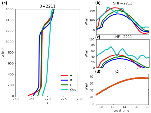
Figure 3Potential temperature (θ) profiles at 20:00 LST (local standard time) (a), SHF (b) and latent heat flux (LHF) (c) diurnal profiles for no anthropogenic heat flux (A, red – , J m−3K−1; B, blue – ) and anthropogenic heat flux (C, green – ) and observations, where panel (d) shows anthropogenic heat flux (Qf) used in the simulation.
Of all surface parameters altered, the largest sensitivity the model showed was to volumetric heat capacity (Ch). Increasing this term decreased maximum SHF, noticeably delayed nocturnal radiative cooling and slightly lowered the temperature through the profile (Fig. 3). This is due to a slower release of outgoing radiation, which is stored longer in urban surfaces. Figure 3 shows the sensitivity to varying surface volumetric heat capacity (J m−3 K−1) between the initial value (2×10⁶) and chosen value (7×10⁶). Higher volumetric heat capacity of the surface causes delayed nocturnal cooling, resulting in higher sensible and latent heat flux in the evening. The surface urban energy balance is also affected by an anthropogenic heat flux which varies seasonally and spatially. A diurnal anthropogenic heat flux which peaks at 70 W m−2 during the daytime and remains around 20 W m−2 in the evening was included in a further simulation. Inclusion of a diurnal Qf profile increased overall temperatures as well as latent and sensible heat fluxes (Fig. 3).
This sensitivity work provides the setup for UCLALES-SALSA in an urban environment and this is utilised for the remainder of results presented below which all include a diurnal Qf profile and heat capacity (Ch) set at 7×10⁶ J m−3 K−1, which is a value typical of concrete (Takebayashi and Moriyama, 2012). The scope for variation of surface parameters within UCLALES is extremely high; therefore, we recognise that within the model framework there is a strong dependence on parameters such as temperature, roughness, heat capacity, albedo and soil moisture. It is also likely that due to the simple homogeneous surface scheme used, some features of the urban environment that are observed cannot be replicated in the chosen model framework. Although the effect of these surface parameters is important to understand, the purpose of this paper is to examine the suitability of using an LES model in investigating urban haze. The parameters chosen here are based on identification of the urban measurement site's characteristics, as well as from chosen literature values and are to the best of the authors' knowledge a fair representation of urban Beijing, as described in the next section.
3.1 Observational data
All measurements used in this study were taken at IAP, Chinese Academy of Sciences, as part of the APHH Beijing campaign. Measurements taken include but are not limited to NR-PM1 (non-refractory PM with a diameter <1 µm) composition and aerosol and black carbon size and concentration measurements at the surface, as well as meteorological measurements at 15 levels on a 320 m tower. Sensible and latent heat flux measurements were calculated and a ceilometer was used to infer PBL height. For more information concerning the measurements taken as well as the APHH project and field campaign, the reader is directed to the Introduction to the special issue “In-depth study of air pollution sources and processes within Beijing and its surrounding region (APHH-Beijing)” by Shi et al. (2019).
3.2 Experimental setup
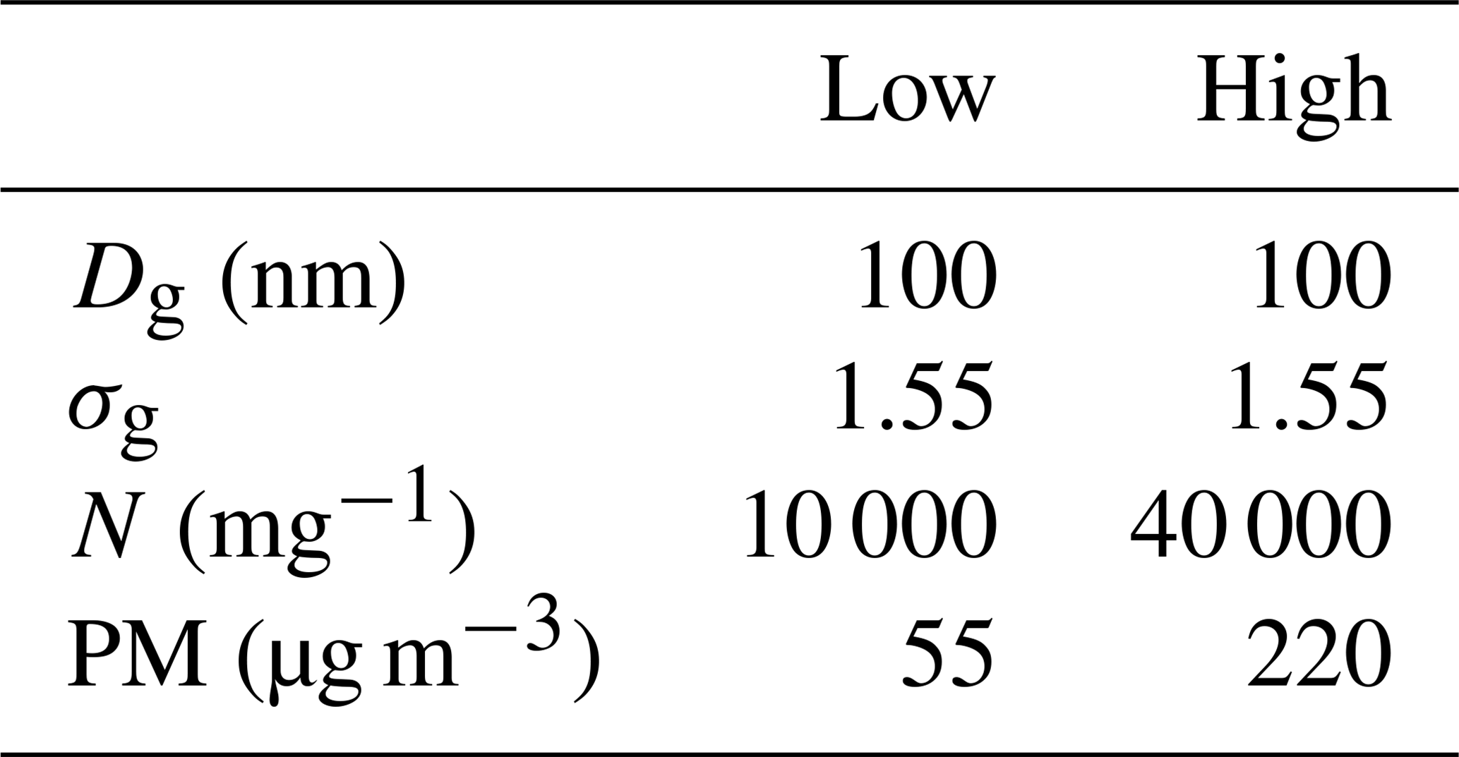
The domain size for all model simulations spanned 5.4 km in the horizontal with a resolution of 30 m, and the model top was set to 1.8 km in the vertical with a resolution of 10 m. The model uses an adaptive time step with a maximum time step of 1 s. A haze period which took place within the APHH winter campaign period from 24 to 26 November 2016 was used to examine the sensitivity of boundary layer meteorology to varying aerosol concentrations. Meteorological data taken from ECMWF-ERA5 reanalysis and tower meteorological data were used to initialise vertical profiles at 08:00 LST on 24, 25 and 26 November. Simulations were run from 08:00 LST for 14 h (22:00 LST) including 1 h spin-up time. Simulations for all days were considered to be cloudless. Case studies for each day were simulated and compared to each other and are described as follows: case 1 – no aerosols, case 2 – high and low aerosol loading, case 3 – aerosol vertical profiles. For case 2, aerosol vertical profiles were constant in the column, whereas case 3 examined the impact of including a varying aerosol vertical profile. Aerosol size distribution parameters and volume fraction of aerosol components were the same for all simulations, detailed in Tables 1 and 2. The values for aerosol size distribution data used were measured by a scanning mobility particle sizer (SMPS) and aerosol composition measurements were taken with an aerosol mass spectrometer (AMS). All in situ measurements were taken at IAP and values used were averaged between 07:30 and 08:30 LST on 24 November 2016. In all cases, BC can be considered to be the primary absorbing aerosol, with sulfate (), nitrate () and ammonium () strongly scattering and organics (OC) predominantly scattering with a small absorbing component. Aerosol growth is considered through the processes of coagulation and water condensation, but semi-volatile condensation is not considered. Both wet and dry deposition are switched off in all simulations.
Table 1Real (n) and imaginary (k) refractive indices across 13 shortwave wavelengths (λ for all aerosol components considered for aerosol–radiation interactions in this simulation.
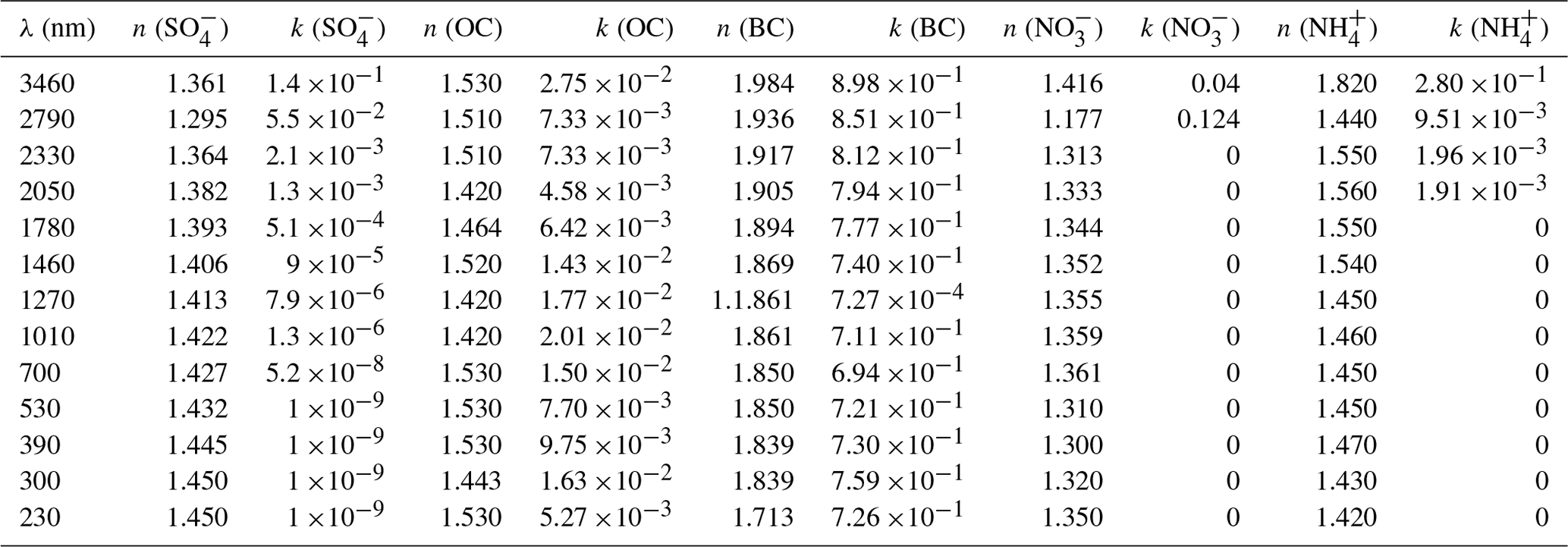
Table 2Size distribution parameters initialised for simulations examining measured aerosol feedback on meteorology. Dg (geometric mean diameter), σg (geometric standard deviation), N (number concentration), as well as calculated surface PM concentration for low and high aerosol simulations.
The results highlighted in this section aim to test the sensitivity of the newly coupled aerosol–radiation scheme in UCLALES-SALSA to aerosol loading, using meteorological conditions, urban characteristics and simplified aerosol conditions, associated with Beijing haze episodes. Case 1 shows boundary layer development for 24, 25 and 26 November with no aerosols, case 2 examines the effect of high and low aerosol loading for each of the days, and case 3 focuses on the impact of varying aerosol vertical profiles.
4.1 Case 1 – no aerosols
Simulations in case 1 examine the development of boundary layer dynamics for 24, 25 and 26 November without aerosol–radiation interactions. All 3 d are initialised with different meteorological vertical profiles, taken from ECMWF profiles. On 25 November, there is a strong temperature inversion throughout the whole profile, while on 26 November there is strong vertical wind shear, higher surface humidity and strong stability in the lowest 300 m (Fig. 4). Strong vertical wind shear causes mechanical turbulence, while a strong temperature inversion in the morning can suppress boundary layer development through reducing buoyancy. Figure 4d–f show development of SHF, PBL height and total turbulent kinetic energy (TKE) for the three simulated days with different meteorological conditions initialised in the morning.
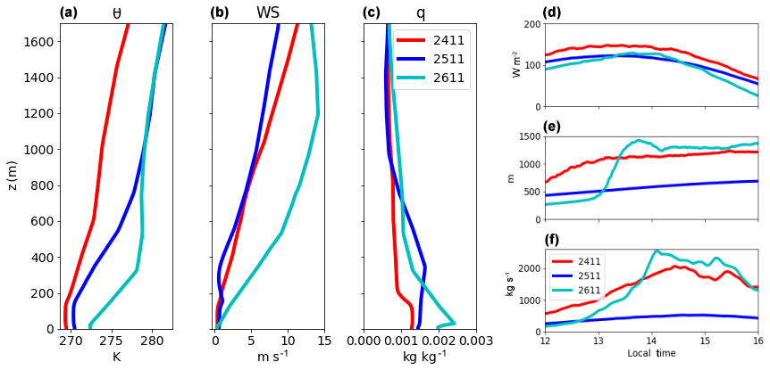
Figure 4(a–c) Initial vertical profiles of potential temperature (θ), wind speed (WS) and total water mixing ratio (q), and (d) sensible heat flux, (e) height of maximum gradient in θ and (f) vertical integral of TKE for 24 November (red), 25 November (blue) and 26 November (turquoise) for simulations with no aerosols (case 1).
SHF is similar in magnitude for all 3 d, while TKE and simulated PBL height are significantly lower for the 25 November simulation. A well-mixed, turbulent boundary layer forms quickly on 24 November; however, on 25 November, a shallow, weakly turbulent boundary layer remains throughout the day, and on 26 November a turbulent boundary layer is much slower to develop (Fig. 4). The changing conditions used here are typical for a Beijing haze episode and show that even without the consideration of aerosols, meteorological conditions can largely affect the diurnal development of boundary layer dynamics.
4.2 Case 2 – high and low aerosol loading
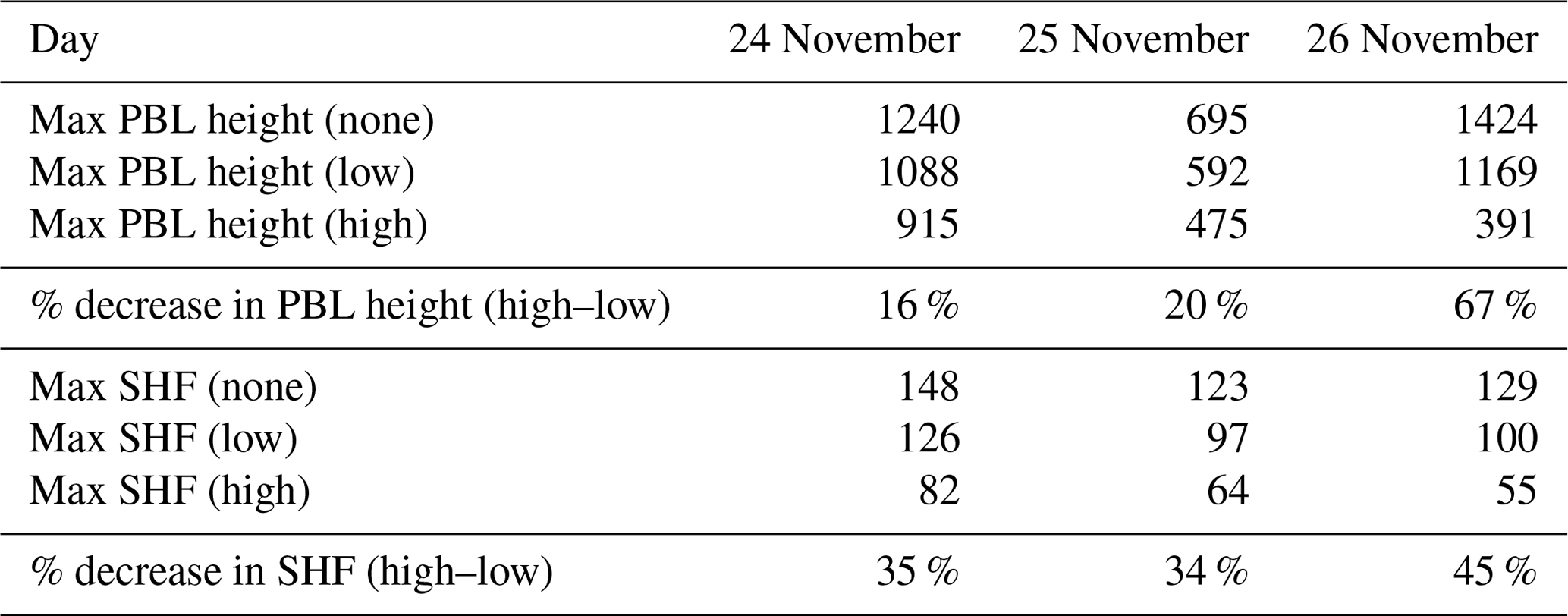
Case 1 shows that simulated boundary layer dynamics are impacted by initial meteorological conditions. In case 2, the sensitivity of boundary layer dynamics to aerosol loading is examined, where aerosol mixing ratios were constant throughout the profile as shown in Fig. 6. Table 4 shows the impact of including high and low aerosol loading on maximum SHF and maximum PBL height between 12:00 and 16:00 LST.
In all cases, inclusion of aerosols causes cooling in the lower planetary boundary layer and warming above it. This is due to the aerosols absorbing and scattering incoming SW radiation (Fig. 5) to reduce the amount of solar radiation reaching the surface. Where there are high concentrations of aerosols through the column, this severely reduces the amount of radiation reaching the surface and consequently causes cooling. Aerosols, specifically black carbon, in the upper layer of the boundary layer will absorb radiation, which causes warming. Including high aerosol concentrations (220 µg m−3) compared to low aerosol concentrations (55 µg m−3) maximised this effect, leading to enhanced temperature inversions, and suppressed PBL development on all 3 d (Table 4).
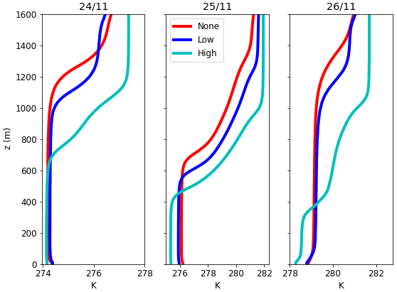
Figure 5Potential temperature profiles at 17:00 LST for 24, 25 and 26 November, with no aerosols (red), low aerosol loading (blue) and high aerosol loading (turquoise).
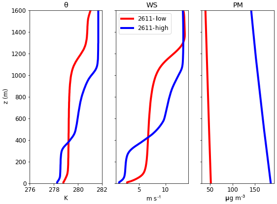
Figure 6Potential temperature (θ), wind speed (WS) and aerosol mass concentration (PM) profiles on 26 November for low (red) and high (blue) aerosol concentrations at 17:00 LST (9 h of simulation).
For the case of 25 November, the PBL is already low due to synoptic conditions and aerosols from the previous day causing strong temperature inversions in the morning. Therefore, even though the aerosols cause cooling in the PBL to the same extent on 26 and 25 November, a strong temperature inversion already exists on 25 November and so the PBL is low even without the inclusion of aerosols.
4.3 Case 3 – aerosol vertical profiles
To assess the sensitivity of the model to a varied aerosol vertical profile, case 3 uses the same setup as case 2 but varies the aerosol mass mixing ratio with altitude, as shown in Fig. 7. This is to assess the impact of high aerosol concentrations aloft in case 2 simulations which may magnify the aerosol–radiation effect, due to higher total loading increasing the total column aerosol optical depth (AOD). In case 3 simulations, total aerosol mass loading throughout the column is ∼22 % less than for case 2 simulations for both high and low aerosol simulations. The aerosol profile was chosen so that at the first time step, the aerosol mass mixing ratio at the surface was the same as those with a constant profile and decreased above the PBL in accordance with the potential temperature profiles, while composition and size remained constant throughout. It should be noted from the varied aerosol vertical profile simulations that total aerosol mass mixing ratio decreases by about 5 % over the course of the day. This is despite dry deposition not being included in these simulations. This is a result of UCLALES-SALSA using the Ogura–Phillips anelastic approximation for filtering out acoustic waves. The approximation assumes that there are only small variations in pressure and density from static reference values over time. Throughout the day, surface fluxes increase air temperature, while subsidence of air at the model top decreases density (Ogura and Phillips, 1962; Pressel et al., 2015; Byun, 1999). The limitations of the anelastic approximation mean that these changes do not fully feed back to change pressure, and fixed boundary conditions mean that volume remains constant. As the model holds to constant volume rather then constant mass, when SALSA aerosol mass tracers are pulled downward, the total air mass increases while the mass of aerosols remains the same; this causes the apparent decrease in aerosol mass mixing ratio (Fig. 7). We consider this to be a limitation of using a meteorological model for air quality analysis; however, as the relative reduction is the same for different meteorological conditions, comparisons between different cases can still be performed.
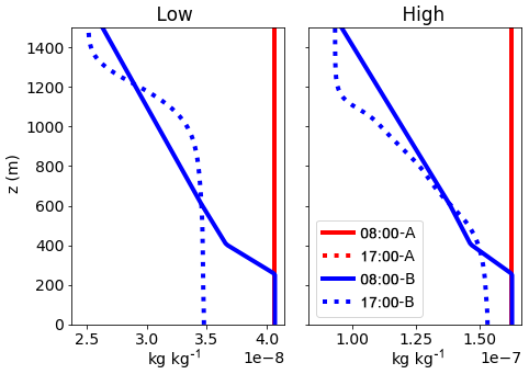
Figure 7Aerosol mass mixing ratio vertical profiles for low and high aerosol loading simulations on 26 November, for constant aerosol profile (red) and vertically varying aerosol profiles (blue) at initial time step (solid) and after 9 h simulation (dashed). For the case of the constant vertical profiles (red lines), the aerosol mass mixing ratio remains constant through time and so the dashed red lines are hidden behind the solid red ones.
Figure 8 shows simulation results of potential temperature and aerosol number mixing ratio at 17:00 LST (9 h of simulation) for constant and varied aerosol vertical profiles at high concentrations for 24 and 26 November. When a varied aerosol profile is included, vertical mixing of aerosol occurs, resulting in a difference in the aerosol vertical profile on each day at 17:00 LST due to the difference in meteorology. The difference between the aerosol profiles over time shows the modelled meteorological feedback on aerosol mixing ratios.
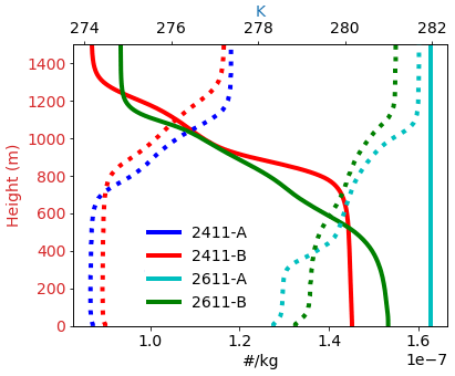
Figure 8Number mixing ratio (solid) and potential temperature (dashed) vertical profiles at 17:00 LST for constant vertical aerosol profiles on 24 November (blue) and 26 November (turquoise) and varied aerosol vertical profiles on 24 November (red) and 26 November (green). The mixing ratios for constant aerosol vertical profiles (blue and turquoise) remain constant in time for both simulations; the solid blue line is equivalent to the solid turquoise line.
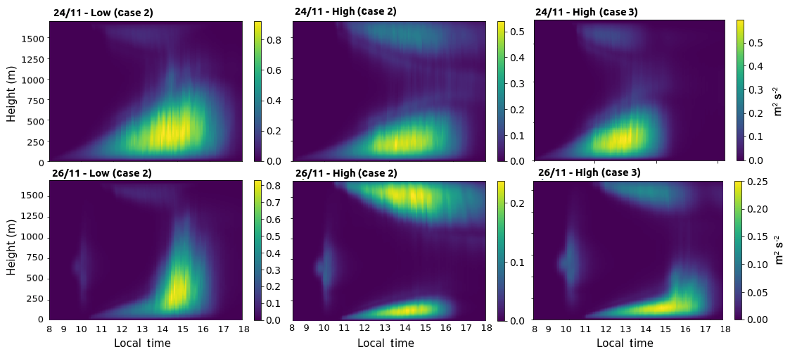
Figure 9Variance in vertical velocity () on 24 and 26 November for case 2 (low and high aerosol loading) and case 3 (high aerosol loading).
Figure 9 compares the variance in vertical velocity () for low and high aerosol loading throughout the profile and at high aerosol loading at the surface only for the 24 and 26 November simulations and shows that high aerosol loading, both throughout the column and at the surface, decreases at 500–750 m in the afternoon of both 24 November and 26 November. It also shows the effect of high aerosol loading throughout the column, which causes an increase in close to the model top, with the varied aerosol vertical profiles minimising this effect as the aerosols increase vertical velocity, through creating a turbulent layer. This is due to aerosol warming aloft close to the model top causing stratification of the layer. Reduced aerosol concentrations in the entire column indicate that more solar radiation reaches the surface in the varied vertical aerosol profile case, increasing buoyant turbulence and vertical velocity at lower altitudes.
The results highlighted above show the use of a novel coupled LES–aerosol radiation model to investigate haze in the urban environment of Beijing. Simulated sensitivity to urban surface parameters is high and these will be different for other urban locations. It is therefore necessary to evaluate and tune these parameters to observations in specific environments in order to use an LES model to fully explore boundary layer dynamic sensitivities. Aerosol–radiation interactions were tested for the first time in the model framework and showed that sensitivity of boundary layer meteorology and turbulence to aerosol loading was strong while also being dependent on initial meteorological conditions.
5.1 Sensitivity to meteorology
Case 1 identifies the importance of meteorological conditions on boundary layer dynamics throughout the day. Many observations in Beijing found that meteorological conditions are a main driver for both the onset and longevity of haze. Large-scale synoptic conditions such as southerly winds and low pressure often pre-empt pollution episodes which tend to occur every 4–7 d during wintertime in Beijing (C. Liu et al., 2018; Wang et al., 2019). These conditions are associated with the beginning of “haze” as the switch in meteorological conditions from strong northwesterly to southerly winds advects pollution from surrounding provinces into Beijing. This change is also associated with a low pressure field within the city, where stagnant air becomes trapped and the dispersion of pollutants is inhibited (Gao et al., 2016).
The initial meteorological profiles for the simulations on 24 November are taken prior to the onset of the haze and are associated with clean conditions. This is likely the reason for the quick turbulent boundary layer development along with high TKE and SHF throughout the day. Observations show that aerosol concentrations begin to build up around midday on 24 November and remain constant until the afternoon of 25 November when concentrations build up rapidly, peaking overnight on 25 November and remaining high until the afternoon of 26 November. Therefore, the initial conditions used in the simulation of 25 November will have been slightly affected by aerosol–radiation interactions of the previous evening. Aerosol–radiation interactions reduce the amount of solar radiation reaching the surface which causes cooling; simultaneously, black carbon aerosols will absorb radiation at the top of the PBL. Although absorption by BC occurs throughout the column, several studies have shown that due to the higher incidence of solar radiation and lower density of air, BC causes warming at PBL top to a greater extent than at the surface (Ding et al., 2016). Overall, this causes a temperature inversion during periods where pollution is high and causes a shallow PBL to form during the day. This leads to stagnant conditions and can affect the meteorology of the next day, particularly when aerosols are suppressed in a shallow PBL. However, frequently during wintertime in Beijing, changes in pressure can cause warm polluted air to converge with cold clean air to create a layer of cold air under a layer of warm air. These conditions often pre-empt pollution episodes in Beijing and favour the accumulation of pollutants in a shallow boundary layer. A combination of these factors explains the strong temperature inversion in the morning and results in a shallow turbulent boundary layer forming in these simulations, with lower turbulent kinetic energy compared to the 24 November simulation (Fig. 4).
5.2 Sensitivity to aerosol loading
Aerosol–radiation interactions cause a reduction in SHF, surface SW radiation and TKE, resulting in a reduction in the daily maximum PBL height for all 3 d examined. In these simulations, the aerosols interact with radiation to cause heating and cooling in different layers which perturbs the temperature profile of the PBL and decreases the sensible heat flux term. The aerosols also take up water to a small extent which decreases latent heat. These effects lead to decreased turbulence in the PBL. High aerosol concentrations enhance this effect due to an increased number of aerosols interacting with radiation. This leads to a reduction in maximum SHF of 44, 33 and 45 W m−2 for high compared to low aerosol loading simulations on 24, 25 and 26 November, respectively. However, results from case 2 show a variation in the magnitude of the aerosol–radiation effect with a larger impact on maximum PBL height for high aerosol simulations on 26 November compared to 24 and 25 November (Table 3). Including high aerosols on 26 November causes >1 ∘C of daytime cooling in the lowest 300 m compared to 0.3 ∘C of cooling on 24 November (Figs. 5 and 6). The larger degree of cooling on 26 November leads to a larger reduction in buoyant turbulence and prevents the full growth of a deeply turbulent boundary layer to a larger extent on 26 November.
Table 3Volume fraction of aerosols included in SALSA for all simulations in case 2 and case 3.
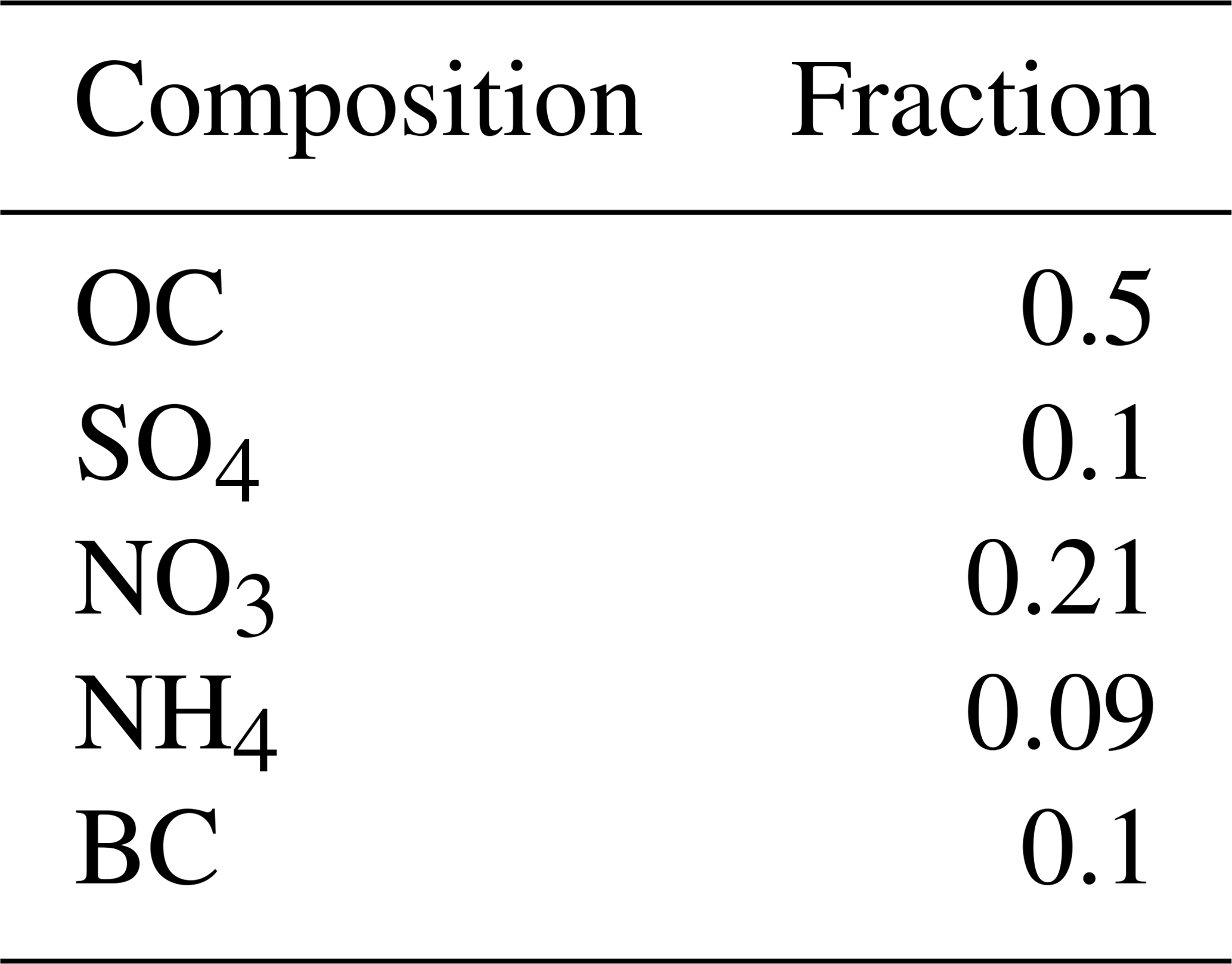
Table 4Change in maximum PBL height (taken as the height between 12:00 and 16:00 LST with a maximum gradient in potential temperature) and SHF for all 3 d with high and low aerosol loading.
High aerosol concentrations are known to stabilise the boundary layer through the reduction of vertical transport of momentum to the surface (Jacobson and Kaufman, 2006). This can reduce wind speeds at lower altitudes and thus decrease wind shear and the shear component of TKE. In case 2, high aerosol loadings reduce surface wind speeds, wind shear and surface frictional velocity (u∗) for all 3 d, with a greater reduction on 26 November compared to 24 and 25 November. High aerosol loading also causes a reduction in the variance of vertical velocity (), which can be considered a measure of turbulence (Stull, 2015). On both 24 and 26 November, simulations with high aerosol loading caused a reduction in the magnitude of particularly between 500 and 800 m. On 24 November, the decrease at the surface at is ∼40 %, while on 26 November the reduction is 75 %. In the case of 26 November, this is accompanied by increased values of in the upper layers close to the model top, which results in two turbulent layers forming separated by a stable layer (Fig. 9).
In these simulations, aerosol profiles are constant through the column and high aerosol concentrations aloft. Figure 8 shows that high aerosol throughout the column causes warming in the upper layers and cooling in the lower layers, which causes strong stability throughout the profile. In reality, aerosols tend to be concentrated closer to the surface and within the boundary layer, although occasionally in Beijing regional transport can lead to higher aerosol concentrations aloft. Therefore, case 3 investigated the effect of limiting pollution to the surface by including aerosol vertical varying profiles.
5.3 Vertical profiles
Case 3 examined the impact of meteorological feedback on aerosol vertical mixing for high and low aerosol loading simulations by including aerosol vertical profiles on 24 and 26 November. Simulations with a varied vertical aerosol profile had the same aerosol concentrations at the surface as the high aerosol simulations in case 2 but reduced concentrations at higher altitudes (Fig. 7). This resulted in a small increase in maximum SHF (∼7 W m−2) on both 24 and 26 November. For 26 November, limiting high aerosol loading to the surface results in an afternoon increase in turbulence up to 500 m. Furthermore, the effect of high aerosols throughout the column (case 2) resulted in a highly turbulent layer at model top and a large reduction in surface wind speed on 26 November (Fig. 9). As this turbulent layer is significantly reduced with lower aerosols aloft, this effect may be considered to be an artefact of aerosol loading at high altitudes which is not often observed in poor-air-quality events during wintertime in China. However, overall, the contribution of the shear term to turbulence is minimal compared to the buoyancy term, which is greatly reduced by high aerosol loading in both case 2 and case 3. The high aerosol loading in case 2 has a larger effect on boundary layer development than the effect of varying the aerosol vertical profile in case 3. Therefore, we can consider the change in the thermal profile of the atmosphere, due to high concentrations of aerosols increasing aerosol–radiation interactions, to be the prominent cause of the reduction in SHF and PBL height (Table 3).
The large degree of cooling on 26 November compared to 24 November is due to the effects of initial meteorology feeding back on aerosol–radiation interactions. Figure 8 shows potential temperature and aerosol number mixing ratio vertical profiles for each case (after 9 h of simulation) under high aerosol loading at the surface only (red and green lines) and throughout the profile (blue and turquoise lines). After 9 h of simulation (17:00 LST), surface aerosol concentrations on 26 November are higher than on 24 November. This is due to aerosol–radiation interactions and initial meteorological conditions on 26 November resulting in a shallower PBL (Table 3). This shows the ability of UCLALES-SALSA to simulate the aerosol–radiation–meteorology feedback loop and that the feedback effect can have a significant impact on aerosol surface concentrations, which will consequently feed back further on atmospheric stability.
UCLALES-SALSA was set up to model an urban environment for the first time, in order to investigate the impact of aerosol–radiation interactions on urban haze. During setup, sensitivity to urban surface parameters was shown to be high and accounted for the slower release of heat throughout the day as observed in urban Beijing. Inclusion of a diurnal anthropogenic heat flux in simulations resulted in a warmer environment typical of an urban heat island. Given the sensitivity to such parameters, accurate measurements of these properties can be considered paramount in order to improve modelling of the urban environment. Turbulent motion throughout the day in each simulation is further impacted by initial meteorological profiles. Conditions associated with clean periods in Beijing allow for the development of a highly turbulent boundary layer, while strong morning temperature inversions prevent the growth of a turbulent boundary layer throughout the day. Aerosol–radiation interactions in all cases decreases SHF, TKE and PBL height, in addition to causing cooling at the surface and reducing surface wind speeds. All simulations also show a large sensitivity to aerosol loading, with more than a one-third reduction in SHF due to high aerosol loading in all simulations. Through comparing simulations with and without aerosol vertical profiles (case 3), we observe that on 26 November the simulated development of a turbulent boundary layer in the afternoon is impacted by high aerosol loading aloft (case 2). This is due to aerosols at high altitudes reducing mechanical shear as well as the reduction in buoyancy. However, overall, the effect of including a vertical aerosol profile is minimal compared to the effect of overall aerosol loading, which suggests a higher effect of surface aerosols.
The sensitivity work outlined above aims to isolate the aerosol and dynamical effects on pollution episodes through using a specific period with varying meteorological conditions and simplified aerosol conditions. LES models are limited in their ability to represent changing synoptic conditions without additionally forcing or nudging simulated profiles with mesoscale model results or through observations. However, these simulations do show the sensitivity to and importance of meteorological conditions in the development of boundary layer turbulence in Beijing in addition to assessing the importance of aerosol loading on the aerosol–meteorology feedback loop and the impact on PBL turbulent statistics. The aerosol feedback loop is thought to have the largest impact on haze episodes during the cumulative and dissipation stages of the pollution episode. Future work will focus particularly on these stages and the impact of aerosol–radiation–meteorology interactions. As aerosol optical properties play an important role in the feedback, future work will also take advantage of the SALSA framework to vary aerosol optical properties in a case study of Beijing haze.
The input data for the simulations performed in this study can now be found at https://github.com/ja-slater/UCLALES-SALSA-Beijing (last access: 12 January 2017). All data used for comparison were taken as part of the APHH Beijing campaign and are available upon request from the author and acknowledged colleagues.
The idea for the study was conceived by JS, GM and HC. All model simulations were performed by JS with the assistance of JT. JS wrote the paper with input from JT and TK. All co-authors discussed the results and commented on the manuscript.
The authors declare that they have no conflict of interest.
This article is part of the special issue “In-depth study of air pollution sources and processes within Beijing and its surrounding region (APHH-Beijing) (ACP/AMT inter-journal SI)”. It is not associated with a conference.
Model simulations were carried out on the ARCHER UK National Supercomputing Service (http://www.archer.ac.uk, last access: 31 March 2020). We gratefully acknowledge Yele Sun's group and Pingqing Fu's group at IAP for aerosol composition data and tower meteorological data, respectively, as well as Zifa Wang's group at Peking University for aerosol size data and Eiko Nemitz at CEH Edinburgh for heat flux data.
This research has been supported by the National Centre for Atmospheric Science (NCAS), AIRPRO (grant no. NE/N00695X/1) and the Academy of Finland (projects 283031 and 309127).
This paper was edited by Pingqing Fu and reviewed by three anonymous referees.
Ács, F., Mihailović, D. T., and Rajković, B.: A Coupled Soil Moisture and Surface Temperature Prediction Model, J. Appl. Meteorol., 30, 812–822, https://doi.org/10.1175/1520-0450(1991)030<0812:ACSMAS>2.0.CO;2, 1991. a, b
Andrejczuk, M., Gadian, A., and Blyth, A.: Numerical simulations of stratocumulus cloud response to aerosol perturbation, Atmos. Res., 140–141, 76–84, https://doi.org/10.1016/j.atmosres.2014.01.006, 2014. a
Bellon, G. and Stevens, B.: Using the sensitivity of large-eddy simulations to evaluate atmospheric boundary layer models, J. Atmos. Sci., 69, 1582–1601, https://doi.org/10.1175/JAS-D-11-0160.1, 2012. a
Bond, T. C. and Bergstrom, R. W.: Light absorption by carbonaceous particles: An investigative review, Aerosol Sci. Tech., 40, 27–67, https://doi.org/10.1080/02786820500421521, 2006. a
Byun, D. W.: Dynamically consistent formulations in meteorological and air quality models for multiscale atmospheric studies. Part II: Mass conservation issues, J. Atmos. Sci., 56, 3808–3820, https://doi.org/10.1175/1520-0469(1999)056<3808:DCFIMA>2.0.CO;2, 1999. a
Ding, A. J., Huang, X., Nie, W., Sun, J. N., Kerminen, V. M., Petäjä, T., Su, H., Cheng, Y. F., Yang, X. Q., Wang, M. H., Chi, X. G., Wang, J. P., Virkkula, A., Guo, W. D., Yuan, J., Wang, S. Y., Zhang, R. J., Wu, Y. F., Song, Y., Zhu, T., Zilitinkevich, S., Kulmala, M., and Fu, C. B.: Enhanced haze pollution by black carbon in megacities in China, Geophys. Res. Lett., 43, 2873–2879, https://doi.org/10.1002/2016GL067745, 2016. a, b
Dou, J., Wang, Y., Bornstein, R., and Miao, S.: Observed spatial characteristics of Beijing urban climate impacts on summer thunderstorms, J. Appl. Meteorol. Clim., 54, 94–105, https://doi.org/10.1175/JAMC-D-13-0355.1, 2015. a
Dou, J., Grimmond, S., Cheng, Z., Miao, S., Feng, D., and Liao, M.: Summertime surface energy balance fluxes at two Beijing sites, Int. J. Climatol., 39, 2793–2810, https://doi.org/10.1002/joc.5989, 2019. a
Fu, Q. and Liou, K. N.: Parameterization of the Radiative Properties of Cirrus Clouds, J. Atmos. Sci., 50, 2008–2025, https://doi.org/10.1175/1520-0469(1993)050<2008:POTRPO>2.0.CO;2, 1993. a, b
Gao, M., Carmichael, G. R., Wang, Y., Saide, P. E., Yu, M., Xin, J., Liu, Z., and Wang, Z.: Modeling study of the 2010 regional haze event in the North China Plain, Atmos. Chem. Phys., 16, 1673–1691, https://doi.org/10.5194/acp-16-1673-2016, 2016. a
Gao, Y., Zhang, M., Liu, Z., Wang, L., Wang, P., Xia, X., Tao, M., and Zhu, L.: Modeling the feedback between aerosol and meteorological variables in the atmospheric boundary layer during a severe fog–haze event over the North China Plain, Atmos. Chem. Phys., 15, 4279–4295, https://doi.org/10.5194/acp-15-4279-2015, 2015. a, b
Grimmond, C. S. B. and Oke, T. R.: Heat Storage in Urban Areas: Local-Scale Observations and Evaluation of a Simple Model, J. Appl. Meteorol., 38, 922–940, https://doi.org/10.1175/1520-0450(1999)038<0922:HSIUAL>2.0.CO;2, 1999. a
Hu, D., Yang, L., Zhou, J., and Deng, L.: Estimation of urban energy heat flux and anthropogenic heat discharge using aster image and meteorological data: case study in Beijing metropolitan area, J. Appl. Remote Sens., 6, 063559 https://doi.org/10.1117/1.JRS.6.063559, 2012. a
Ikeda, R., Kusaka, H., Iizuka, S., and Boku, T.: Development of Urban Meteorological LES model for thermal environment at city scale, ICUC9 – 9th International Conference on Urban Climate jointly with 12th Symposium on the Urban Environment Development, 20–24 July 2012, Toulouse France, 2012. a
Jacobson, M. Z. and Kaufman, Y. J.: Wind reduction by aerosol particles, Geophys. Res. Lett., 33, 1–6, https://doi.org/10.1029/2006GL027838, 2006. a
Kokkola, H., Korhonen, H., Lehtinen, K. E. J., Makkonen, R., Asmi, A., Järvenoja, S., Anttila, T., Partanen, A.-I., Kulmala, M., Järvinen, H., Laaksonen, A., and Kerminen, V.-M.: SALSA – a Sectional Aerosol module for Large Scale Applications, Atmos. Chem. Phys., 8, 2469–2483, https://doi.org/10.5194/acp-8-2469-2008, 2008. a, b
Kokkola, H., Kühn, T., Laakso, A., Bergman, T., Lehtinen, K. E. J., Mielonen, T., Arola, A., Stadtler, S., Korhonen, H., Ferrachat, S., Lohmann, U., Neubauer, D., Tegen, I., Siegenthaler-Le Drian, C., Schultz, M. G., Bey, I., Stier, P., Daskalakis, N., Heald, C. L., and Romakkaniemi, S.: SALSA2.0: The sectional aerosol module of the aerosol–chemistry–climate model ECHAM6.3.0-HAM2.3-MOZ1.0, Geosci. Model Dev., 11, 3833–3863, https://doi.org/10.5194/gmd-11-3833-2018, 2018. a
Liu, B., Ma, Y., Gong, W., Zhang, M., and Shi, Y.: The relationship between black carbon and atmospheric boundary layer height, Atmos. Pollut. Res., 10, 65–72, https://doi.org/10.1016/j.apr.2018.06.007, 2019. a
Liu, C., Huang, J., Fedorovich, E., Hu, X.-M., Wang, Y., and Lee, X.: The Effect of Aerosol Radiative Heating on Turbulence Statistics and Spectra in the Atmospheric Convective Boundary Layer: A Large-Eddy Simulation Study, Atmosphere, 9, 347, https://doi.org/10.3390/atmos9090347, 2018. a
Liu, Q., Ma, T., Olson, M. R., Liu, Y., Zhang, T., Wu, Y., and Schauer, J. J.: Temporal variations of black carbon during haze and non-haze days in Beijing, Sci. Rep., 6, 33331, https://doi.org/10.1038/srep33331, 2016. a
Liu, Q., Jia, X., Quan, J., Li, J., Li, X., Wu, Y., Chen, D., Wang, Z., and Liu, Y.: New positive feedback mechanism between boundary layer meteorology and secondary aerosol formation during severe haze events, Sci. Rep., 8, 1–8, https://doi.org/10.1038/s41598-018-24366-3, 2018. a, b, c, d
Luan, T., Guo, X., Guo, L., and Zhang, T.: Quantifying the relationship between PM2.5 concentration, visibility and planetary boundary layer height for long-lasting haze and fog–haze mixed events in Beijing, Atmos. Chem. Phys., 18, 203–225, https://doi.org/10.5194/acp-18-203-2018, 2018. a
Mazoyer, M., Lac, C., Thouron, O., Bergot, T., Masson, V., and Musson-Genon, L.: Large eddy simulation of radiation fog: impact of dynamics on the fog life cycle, Atmos. Chem. Phys., 17, 13017–13035, https://doi.org/10.5194/acp-17-13017-2017, 2017. a
Mukherjee, S., Schalkwijk, J., and Jonker, H. J. J.: Predictability of dry convective boundary layers: an LES study, J. Atmos. Sci., 73, 2715–2725, https://doi.org/10.1175/JAS-D-15-0206.1, 2016. a
Ogura, Y. and Phillips, N. A.: Scale Analysis of Deep and Shallow Convection in the Atmosphere, J. Atmos. Sci., 19, 173–179, https://doi.org/10.1175/1520-0469(1962)019<0173:saodas>2.0.co;2, 1962. a
Oke, T.: The energetic basis of the urban heat island, Q. J. Roy. Meteor. Soc., 108, 1–24, 1982. a, b
Petäjä, T., Järvi, L., Kerminen, V.-M., Ding, A. J., Sun, J. N., Nie, W., Kujansuu, J., Virkkula, A., Yang, X., Fu, C. B., Zilitinkevich, S., and Kulmala, M.: Enhanced air pollution via aerosol-boundary layer feedback in China, Sci. Rep., 6, 18998, https://doi.org/10.1038/srep18998, 2016. a
Pressel, K., Kaul, C., Schneider, T., Tan, Z., and Mishra, S.: Large eddy simulation in an anelastic framework with closed water and entropy balances, J. Adv. Model. Earth Syst., 7, 1425–1456, https://doi.org/10.1002/2017MS001065, 2015. a
Schwarz, N., Lautenbach, S., and Seppelt, R.: Exploring indicators for quantifying surface urban heat islands of European cities with MODIS land surface temperatures, Remote Sens. Environ., 115, 3175–3186, https://doi.org/10.1016/j.rse.2011.07.003, 2011. a
Shi, Z., Vu, T., Kotthaus, S., Harrison, R. M., Grimmond, S., Yue, S., Zhu, T., Lee, J., Han, Y., Demuzere, M., Dunmore, R. E., Ren, L., Liu, D., Wang, Y., Wild, O., Allan, J., Acton, W. J., Barlow, J., Barratt, B., Beddows, D., Bloss, W. J., Calzolai, G., Carruthers, D., Carslaw, D. C., Chan, Q., Chatzidiakou, L., Chen, Y., Crilley, L., Coe, H., Dai, T., Doherty, R., Duan, F., Fu, P., Ge, B., Ge, M., Guan, D., Hamilton, J. F., He, K., Heal, M., Heard, D., Hewitt, C. N., Hollaway, M., Hu, M., Ji, D., Jiang, X., Jones, R., Kalberer, M., Kelly, F. J., Kramer, L., Langford, B., Lin, C., Lewis, A. C., Li, J., Li, W., Liu, H., Liu, J., Loh, M., Lu, K., Lucarelli, F., Mann, G., McFiggans, G., Miller, M. R., Mills, G., Monk, P., Nemitz, E., O'Connor, F., Ouyang, B., Palmer, P. I., Percival, C., Popoola, O., Reeves, C., Rickard, A. R., Shao, L., Shi, G., Spracklen, D., Stevenson, D., Sun, Y., Sun, Z., Tao, S., Tong, S., Wang, Q., Wang, W., Wang, X., Wang, X., Wang, Z., Wei, L., Whalley, L., Wu, X., Wu, Z., Xie, P., Yang, F., Zhang, Q., Zhang, Y., Zhang, Y., and Zheng, M.: Introduction to the special issue “In-depth study of air pollution sources and processes within Beijing and its surrounding region (APHH-Beijing)”, Atmos. Chem. Phys., 19, 7519–7546, https://doi.org/10.5194/acp-19-7519-2019, 2019. a
Stevens, B., Lenschow, D. H., Vali, G., Gerber, H., Bandy, A., Blomquist, B., Brenguier, J. L., Bretherton, C. S., Burnet, F., Campos, T., Chai, S., Faloona, I., Friesen, D., Haimov, S., Laursen, K., Lilly, D. K., Loehrer, S. M., Malinowski, S. P., Morley, B., Petters, M. D., Rogers, D. C., Russell, L., Savic-Jovcic, V., Snider, J. R., Straub, D., Szumowski, M. J., Takagi, H., Thornton, D. C., Tschudi, M., Twohy, C., Wetzel, M., and Van Zanten, M. C.: Dynamics and Chemistry of Marine Stratocumulus – DYCOMS-II, B. Am. Meteorol. Soc., 84, 579–593, https://doi.org/10.1175/BAMS-84-5-579, 2003. a
Stevens, B., Moeng, C.-H., Ackerman, A. S., Bretherton, C. S., Chlond, A., de Roode, S., Edwards, J., Golaz, J.-C., Jiang, H., Khairoutdinov, M., Kirkpatrick, M. P., Lewellen, D. C., Lock, A., Müller, F., Stevens, D. E., Whelan, E., and Zhu, P.: Evaluation of Large-Eddy Simulations via Observations of Nocturnal Marine Stratocumulus, Mon. Weather Rev., 133, 1443–1462, https://doi.org/10.1175/MWR2930.1, 2005. a
Stull, R.: Atmospheric Boundary Layer, in: Practical Meteorology: An Algebra-based Survey of Atmospheric Science, Sundog Publishing, 453–458, 2015. a
Sullivan, P. P. and Patton, E. G.: The Effect of Mesh Resolution on Convective Boundary Layer Statistics and Structures Generated by Large-Eddy Simulation, J. Atmos. Sci., 68, 2395–2415, https://doi.org/10.1175/JAS-D-10-05010.1, 2011. a
Takebayashi, H. and Moriyama, M.: Study on Surface Heat Budget of Various Pavements for Urban Heat Island Mitigation, Adv. Mater. Sci. Eng., 523051, https://doi.org/10.1155/2012/523051, 2012. a
Tong, S., Wong, N. H., Tan, C. L., Jusuf, S. K., Ignatius, M., and Tan, E.: Impact of urban morphology on microclimate and thermal comfort in northern China, Sol. Energ., 155, 212–223, https://doi.org/10.1016/j.solener.2017.06.027, 2017. a
Tonttila, J., Maalick, Z., Raatikainen, T., Kokkola, H., Kühn, T., and Romakkaniemi, S.: UCLALES–SALSA v1.0: a large-eddy model with interactive sectional microphysics for aerosol, clouds and precipitation, Geosci. Model Dev., 10, 169–188, https://doi.org/10.5194/gmd-10-169-2017, 2017. a, b, c, d, e, f
Wang, L., Liu, J., Gao, Z., Li, Y., Huang, M., Fan, S., Zhang, X., Yang, Y., Miao, S., Zou, H., Sun, Y., Chen, Y., and Yang, T.: Vertical observations of the atmospheric boundary layer structure over Beijing urban area during air pollution episodes, Atmos. Chem. Phys., 19, 6949–6967, https://doi.org/10.5194/acp-19-6949-2019, 2019. a, b
Wu, J., Bei, N., Hu, B., Liu, S., Zhou, M., Wang, Q., Li, X., Liu, L., Feng, T., Liu, Z., Wang, Y., Cao, J., Tie, X., Wang, J., Molina, L. T., and Li, G.: Aerosol–radiation feedback deteriorates the wintertime haze in the North China Plain, Atmos. Chem. Phys., 19, 8703–8719, https://doi.org/10.5194/acp-19-8703-2019, 2019. a, b
Xie, M., Liao, J., Wang, T., Zhu, K., Zhuang, B., Han, Y., Li, M., and Li, S.: Modeling of the anthropogenic heat flux and its effect on regional meteorology and air quality over the Yangtze River Delta region, China, Atmos. Chem. Phys., 16, 6071–6089, https://doi.org/10.5194/acp-16-6071-2016, 2016. a
Yang, L., Qian, F., Song, D. X., and Zheng, K. J.: Research on Urban Heat-Island Effect, Procedia Engineer., 169, 11–18, https://doi.org/10.1016/j.proeng.2016.10.002, 2016. a, b
Zhang, X. Y., Wang, J. Z., Wang, Y. Q., Liu, H. L., Sun, J. Y., and Zhang, Y. M.: Changes in chemical components of aerosol particles in different haze regions in China from 2006 to 2013 and contribution of meteorological factors, Atmos. Chem. Phys., 15, 12935–12952, https://doi.org/10.5194/acp-15-12935-2015, 2015. a
Zhang, Z., Zhang, X., Zhang, Y., Wang, Y., Zhou, H., Shen, X., Che, H., Sun, J., and Zhang, L.: Characteristics of chemical composition and role of meteorological factors during heavy aerosol pollution episodes in northern Beijing area in autumn and winter of 2015, Tellus B, 69, 1347484, https://doi.org/10.1080/16000889.2017.1347484, 2017. a
Zhong, J., Zhang, X., Wang, Y., Liu, C., and Dong, Y.: Heavy aerosol pollution episodes in winter Beijing enhanced by radiative cooling effects of aerosols, Atmos. Res., 209, 59–64, https://doi.org/10.1016/j.atmosres.2018.03.011, 2018a. a
Zhong, J., Zhang, X., Wang, Y., Liu, C., and Dong, Y.: Heavy aerosol pollution episodes in winter Beijing enhanced by radiative cooling effects of aerosols, Atmos. Res., 209, 59–64, https://doi.org/10.1016/j.atmosres.2018.03.011, 2018b. a
Zhong, J., Zhang, X., and Wang, Y.: Relatively weak meteorological feedback effect on PM2.5 mass change in Winter 2017/18 in the Beijing area: Observational evidence and machine-learning estimations, Sci. Total Environ., 664, 140–147, https://doi.org/10.1016/j.scitotenv.2019.01.420, 2019a. a
Zhong, J., Zhang, X., Wang, Y., Wang, J., Shen, X., Zhang, H., Wang, T., Xie, Z., Liu, C., Zhang, H., Zhao, T., Sun, J., Fan, S., Gao, Z., Li, Y., and Wang, L.: The two-way feedback mechanism between unfavorable meteorological conditions and cumulative aerosol pollution in various haze regions of China, Atmos. Chem. Phys., 19, 3287–3306, https://doi.org/10.5194/acp-19-3287-2019, 2019b. a
Zou, J., Sun, J., Ding, A., Wang, M., Guo, W., and Fu, C.: Observation-based estimation of aerosol-induced reduction of planetary boundary layer height, Adv. Atmos. Sci., 34, 1057–1068, https://doi.org/10.1007/s00376-016-6259-8, 2017. a