Modeling the smoky troposphere of the southeast Atlantic: a comparison to ORACLES airborne observations from September of 2016

In the southeast Atlantic, well-defined smoke plumes from Africa advect over marine boundary layer cloud decks; both are most extensive around September, when most of the smoke resides in the free troposphere. A framework is put forth for evaluating the performance of a range of global and regional atmospheric composition models against observations made during the NASA ORACLES (ObseRvations of Aerosols above CLouds and their intEractionS) airborne mission in September 2016. A strength of the comparison is a focus on the spatial distribution of a wider range of aerosol composition and optical properties than has been done previously. The sparse airborne observations are aggregated into approximately 2^∘ grid boxes and into three vertical layers: 3–6 km, the layer from cloud top to 3 km, and the cloud-topped marine boundary layer. Simulated aerosol extensive properties suggest that the flight-day observations are reasonably representative of the regional monthly average, with systematic deviations of 30 % or less. Evaluation against observations indicates that all models have strengths and weaknesses, and there is no single model that is superior to all the others in all metrics evaluated. Whereas all six models typically place the top of the smoke layer within 0–500 m of the airborne lidar observations, the models tend to place the smoke layer bottom 300–1400 m lower than the observations. A spatial pattern emerges, in which most models underestimate the mean of most smoke quantities (black carbon, extinction, carbon monoxide) on the diagonal corridor between 16^∘ S, 6^∘ E, and 10^∘ S, 0^∘ E, in the 3–6 km layer, and overestimate them further south, closer to the coast, where less aerosol is present. Model representations of the above-cloud aerosol optical depth differ more widely. Most models overestimate the organic aerosol mass concentrations relative to those of black carbon, and with less skill, indicating model uncertainties in secondary organic aerosol processes. Regional-mean free-tropospheric model ambient single scattering albedos vary widely, between 0.83 and 0.93 compared with in situ dry measurements centered at 0.86, despite minimal impact of humidification on particulate scattering. The modeled ratios of the particulate extinction to the sum of the black carbon and organic aerosol mass concentrations (a mass extinction efficiency proxy) are typically too low and vary too little spatially, with significant inter-model differences. Most models overestimate the carbonaceous mass within the offshore boundary layer. Overall, the diversity in the model biases suggests that different model processes are responsible. The wide range of model optical properties requires further scrutiny because of their importance for radiative effect estimates.

1 Introduction

The radiative impact of shortwave-absorbing aerosol is subject to large uncertainties over the southeast Atlantic, both in terms of direct radiative effects and in the aerosol's microphysical and radiative interactions with clouds (Myhre et al., 2013; Stier et al., 2013). Efforts to distinguish aerosol effects from meteorology using satellite and reanalysis data suggest that large radiative impacts can be attributed to the shortwave-absorbing aerosol (Adebiyi and Zuidema, 2018; Chand et al., 2009; de Graaf et al., 2019; Lacagnina et al., 2017; Wilcox, 2012), but ultimately models are necessary for attributing radiative impacts to the underlying processes. Recent modeling studies have emphasized both the radiative impact of aerosol–cloud microphysical interactions (Lu et al., 2018) and the effects of free-tropospheric stabilization by smoke (Amiri-Farahani et al., 2020; Gordon et al., 2018; Herbert et al., 2020; Sakaeda et al., 2011). The model process uncertainty, to some extent, reflects the paucity of in situ measurements of aerosol properties in this complex region, in which aerosols and clouds typically occur in the same vertical column, though not necessarily co-located. The southeast Atlantic atmosphere has been known to include elevated levels of biomass-burning aerosol (BBA) since at least Fishman et al. (1991), with subsequent satellite studies documenting the spatial extent and optical depth of the BBA more extensively. These studies confirm that the southeast Atlantic contains a global maximum of BBA present over a lower cloud deck (Waquet et al., 2013). The resulting strong regional climate warming (de Graaf et al., 2014; Peers et al., 2015) is currently not well represented in large-scale models (Stier et al., 2013; Zuidema et al., 2016).

An analysis of surface-based Sun photometer data from Ascension Island (Koch et al., 2009) and a more extensive evaluation using space-based lidar data (Das et al., 2017) conclude that global aerosol models underestimate the amount of BBA brought by long-range transport over the Atlantic. More recent limited in situ aircraft-based observations on black carbon (BC) mass concentrations further confirm the model underestimate of BC over the remote southeast Atlantic (Katich et al., 2018). Katich et al. (2018) compare these observations to a suite of models assembled by the Aerosol Comparisons between Observations and Models (AEROCOM) project, an international initiative encouraging the rigorous comparison of models to observations by imposing standardizations, such as a single fire emissions inventory. While this approach allows for a fruitful attribution of model differences, the assembled global aerosol models reflect their developmental stage in 2012 (Myhre et al., 2013). Aerosol models have become more sophisticated within the past decade, with more parameterizations available that relate aerosol optical properties to their composition and evolution with time.

To date, with the exception of Katich et al. (2018), no assessments have been made of model biomass-burning aerosol optical and compositional properties over the smoky southeast Atlantic. This is in part because until only recently, few in situ measurements were available over the southeast Atlantic. The South African Regional Science Initiative (SAFARI) in 2000–2001 provided important data sets but these were confined to the vicinity of the south African coast (Swap et al., 2003). More significantly, these measurements also preceded the advent of advanced aerosol composition instruments (SP2 and AMS; see Sects. 2.1, 9.1.1, and 9.1.2) and organized international efforts to evaluate global aerosol models systematically.

Motivated in part by the desire to improve model representation of BBA over the southeast Atlantic, a series of field campaigns initiated in the United States, United Kingdom, France, and South Africa gathered aircraft- and surface-based data sets in this climatically important region, beginning in 2016 (Formenti et al., 2019; Redemann, et al., 2020; Zuidema et al., 2016). The first deployment of the NASA ObseRvations of Aerosols above CLouds and their intEractionS (ORACLES) campaign took place in September of 2016. The month of September was chosen because satellite passive remote sensing indicated that this month is the climatological maximum in the spatial overlap of absorbing aerosols above the southeastern Atlantic stratocumulus deck within the annual cycle (Adebiyi et al., 2015), with the large spatial extent of the aerosol driven by strong free-tropospheric winds within an anticyclonic circulation (Adebiyi and Zuidema, 2016). Of the two deployed planes, the NASA P3 was instrumented primarily with in situ instruments and flew in the lower troposphere and mid-troposphere. The NASA ER2 flew at about 20 km altitude with downward-viewing remote sensors. Their data sets have been applied to date to multi-instrument assessment of single scattering albedo (SSA) (Pistone et al., 2019), the above-cloud aerosol optical depths (ACAODs) (LeBlanc et al., 2020), BBA cloud-nucleating activity (Kacarab et al., 2020), and direct aerosol radiative effects (Cochrane et al., 2019).

An important decision made prior to the deployments was to devote approximately half of all research flights to a single pre-established path. The value of unbiased in situ sampling is highlighted in Reddington et al. (2017) as part of the Global Aerosol Synthesis and Science Project. The approach of devoting flight hours specifically to routine flight plans, to facilitate model assessment, was arguably first applied during the VOCALS (VAMOS Ocean-Cloud-Atmosphere-Land Study) experiment in the southeast Pacific (Wood et al., 2011; Wyant et al., 2010, 2015). The aircraft campaigns over the southeast Atlantic differ in that a larger altitude range (up to 6 km) was sampled than during VOCALS, which focused largely on the cloudy boundary layer (Wood et al., 2011). Approximately half of the 15 ORACLES 2016 flights sampled the truly remote southeast Atlantic directly above the heart of the major stratocumulus deck (Fig. 1; Klein and Hartmann, 1993). Other flights acquired more detailed characterization of the atmospheric vertical structure at the expense of a longer range and tended to occur closer to the African coast. Data sets from these flights also contribute to this study.

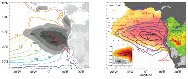
Figure 1 Left: September 2003–2016 WindSat sea surface temperature climatology (colored contours) and 2000–2016 Terra MODIS low cloud fraction climatology (gray shaded contours), with the routine flight track superimposed (red line). Right: September mean climatology of MODIS low-level cloud fraction (2002–2012; blue to black contours, 0.6–1.0 increments of 0.1), fine-mode aerosol optical depth (yellow–red shading indicates 0.25–0.45 in increments of 0.05 and very light black contour lines indicate 0.5–0.7 in increments of 0.1), and fire pixel counts (green–red shading, 50–310 fire counts per 1^∘ box in increments of 50), and ERA-Interim 2002–2012 600 hPa winds (referenced at 10 m s⁻¹). Inset: September mean 6–17^∘ S latitude cross section of Cloud-Aerosol Lidar with Orthogonal Polarization (CALIOP) smoke aerosol count (2006–2012) and CloudSat cloud fraction (2006–2010). The CloudSat cloud fraction is calculated following Stein et al. (2011). The right panel figure was reproduced from Zuidema et al. (2016). © American Meteorological Society. Used with permission.

This paper compares modeled aerosol products with ORACLES 2016 observations. Our study extends more deeply into evaluating the composition, size, and optical properties of the modeled smoke particles above the southeast Atlantic than has been possible to date (described further in Sect. 2.1). The six models participating in this exercise all strive to represent the smoky southeast Atlantic atmosphere and are either versions of the aerosol transport models used for the in-field aerosol forecasts or global and regional models applied for assessing the climate impact of the smoke (Sect. 2.2). Spatiotemporal ranges surrounding the ORACLES flights are chosen to address data sampling challenges (Sect. 3). The extent to which the sampled data represent the climatological monthly mean is assessed in Sect. 4. The model–observation comparisons along the flights begin with the smoke plume altitude (Sect. 5). Aerosol properties are then compared within fixed altitude ranges (Sect. 6). The link between the model biases in the individual aerosol properties is discussed, with the common and divergent findings among the models documented, in order to guide future investigations of the shortcomings of individual models (Sect. 7). A summary is provided in Sect. 8.

Table 1 Specifications of the observations used in this study.

2 Observations and models

2.1 Observations

The instruments and the observed/derived values are described in detail in the Appendix, with general descriptions provided here and summarized in Table 1. BC, a key smoke component that strongly absorbs shortwave absorption, is measured by the Single Particle Soot Photometer (SP2; see Sect. 9.1.1) and organic aerosol masses by a time-of-flight aerosol mass spectrometer (AMS; Sect. 9.1.2). Carbon monoxide (CO), a tracer for air masses originating from combustion, is measured by a Los Gatos Research $\mathrm{CO}/{\mathrm{CO}}_{\mathrm{2}}/{\mathrm{H}}_{\mathrm{2}}\mathrm{O}$ analyzer (Sect. 9.1.7). Aerosol size affects both the optical and the cloud-nucleating properties of BBA. Particles with dry diameters between 60 and 1000 nm are measured with an ultra-high-sensitivity aerosol spectrometer (UHSAS; Sect. 9.1.3). The volumetric arithmetic mean diameter of the accumulation mode is thereafter determined from the cube root of the volume-to-number ratio (V∕N, where V and N are integrals of the volume and number over the UHSAS diameters for each size distribution) after the volume is divided by π∕6.

In situ aerosol scattering is measured by a nephelometer and aerosol absorption by a particle soot absorption photometer (PSAP), both at an instrument relative humidity (RH) that is typically below 40 % (Sect. 9.1.4). From these measurements, extinction coefficient and SSA at 530 nm as well as scattering and absorption Ångström exponents (SAEs, AAEs) across 450–700 nm are derived. Statistics of the aerosol intensive properties (SSA, AE, volumetric mean diameter and an extinction-to-mass ratio) are calculated only from individual measurements with mid-visible dry extinctions greater than 10 Mm⁻¹, thereby reducing the noise apparent at lower aerosol concentrations.

The NASA Langley Research Center High Spectral Resolution Lidar (HSRL-2; Sect. 9.1.5), deployed from the ER2 during 2016, provides an accurate estimate of the elevated smoke plume from above. We use the particulate 532 nm backscattering coefficient and cloud top height, which are among the standard available HSRL-2 products (Burton et al., 2012), to define the bottom and top heights of the smoke plumes. The HSRL-2 employs the HSRL technique (Shipley et al., 1983) to measure calibrated, unattenuated backscatter and aerosol extinction profiles and also has a higher signal-to-noise ratio than the space-based lidars, so it can extensively sample the complete aerosol vertical structure of the aerosol. These mitigate the well-documented low signal-to-noise issue with the space-based Cloud-Aerosol Lidar with Orthogonal Polarization (CALIOP) (Kacenelenbogen et al., 2011; Liu et al., 2015; Lu et al., 2018; Pauly et al., 2019; Rajapakshe et al., 2017).

The HSRL-2 threshold particulate backscattering coefficient is set at 0.25 Mm⁻¹ sr⁻¹. For the layer bottom, we do not search within 300 m of the layer top or beneath the cloud top height. The statistics do not include cases where the smoke base is identified to be higher than 4 km, to avoid artifact noise due to imperfectly cleared cirrus. The backscatter threshold is approximately equivalent to an extinction of 15 Mm⁻¹ for an estimated extinction-to-backscattering ratio of 60 sr, and to a BC mass concentration of 200 ng m⁻³ at standard temperature and pressure (STP, 273 K and 1013 hPa) in our in situ data. The smoke plume is identified within the model data using this BC mass threshold, as the models do not produce backscattering (though the lidar backscattering method does not distinguish between smoke and other aerosols such as marine aerosol). Overall, these are conservative choices emphasizing the clear presence of smoke; 57 % of the 60 s average SP2 measurements in the free troposphere (FT) exceed 200 ng m⁻³ STP. We note that the subjective choice for the threshold affects the gap distance between the smoke plume bottom and the cloud top (Redemann et al., 2020).

In addition, the HSRL-2 532 aerosol extinction profile is used to establish one measure of the ACAOD. Another ACAOD measurement is available from 4STAR (Sect. 9.1.6), a Sun photometer/sky radiometer (LeBlanc et al., 2020) from the low-flying P3 when above cloud top. The variables are selected either because they are robustly observed and pertinent to the absorption of shortwave radiation, and/or are available in most models. Cloud condensation nuclei number concentrations, organic carbon (a derived quantity from the AMS measurements), and cloud properties are not compared in this study.

Table 2 Model specifications.

^∗ Intergovernmental Panel on Climate Change (IPCC) Fifth Assessment Report (AR5) emissions, based on GFED emissions averaged between 1997 and 2002.

2.2 Models

The six assessed models are summarized in Table 2 and detailed in the Appendix. The models applied their native parameterizations and emission inventories, with no standardization applied across the models, in contrast to the planned experiments of the AEROCOM initiative and more in line with the approach of the VOCALS model assessment exercise (Wyant et al., 2010, 2015). As indicated in Table 2, these encompass a range of spatial resolutions, emission frequencies and sources, and meteorological initializations. Three of the models are versions of the field campaign aerosol forecast models but with more sophisticated aerosol physics implemented after the in-field exercise. These are the regional WRF-CAM5 model (Sect. 9.2.1), the global NASA GEOS-5 (Sect. 9.2.2), and the global UK Unified Model (UM; Sect. 9.2.5) in its numerical weather prediction configuration. The three other state-of-the-art models are GEOS-Chem (Sect. 9.2.3), EAM-E3SM (Sect. 9.2.4), and the French regional Aire Limitée Adaptation dynamique Développement InterNational (ALADIN)-Climate model (Sect. 9.2.6; also assessed in Mallet et al. 2019). Additional analysis is performed with two of the models, WRF-CAM5 and GEOS-5, to assess whether the flight days are representative of the monthly mean distributions more typical of Intergovernmental Panel on Climate Change studies.

As noted earlier, a threshold of 200 ng m⁻³ of BC mass concentration at STP is used to locate the model smoke plumes. The only exception is ALADIN-Climate, for which an extinction threshold of 17 Mm⁻¹ at ambient relative humidity, which corresponds to approximately 15 Mm⁻¹ at low RH, is used. As with the observations, the model intensive properties are aggregated only using data with 550 nm extinction (under dry conditions if reported otherwise under the ambient humidity) greater than 10 Mm⁻¹. The observed volume mean diameter is computed from the accumulation mode only, as smaller aerosol sizes contribute little to the overall aerosol volume.

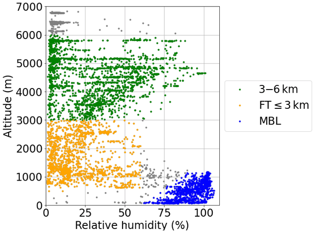
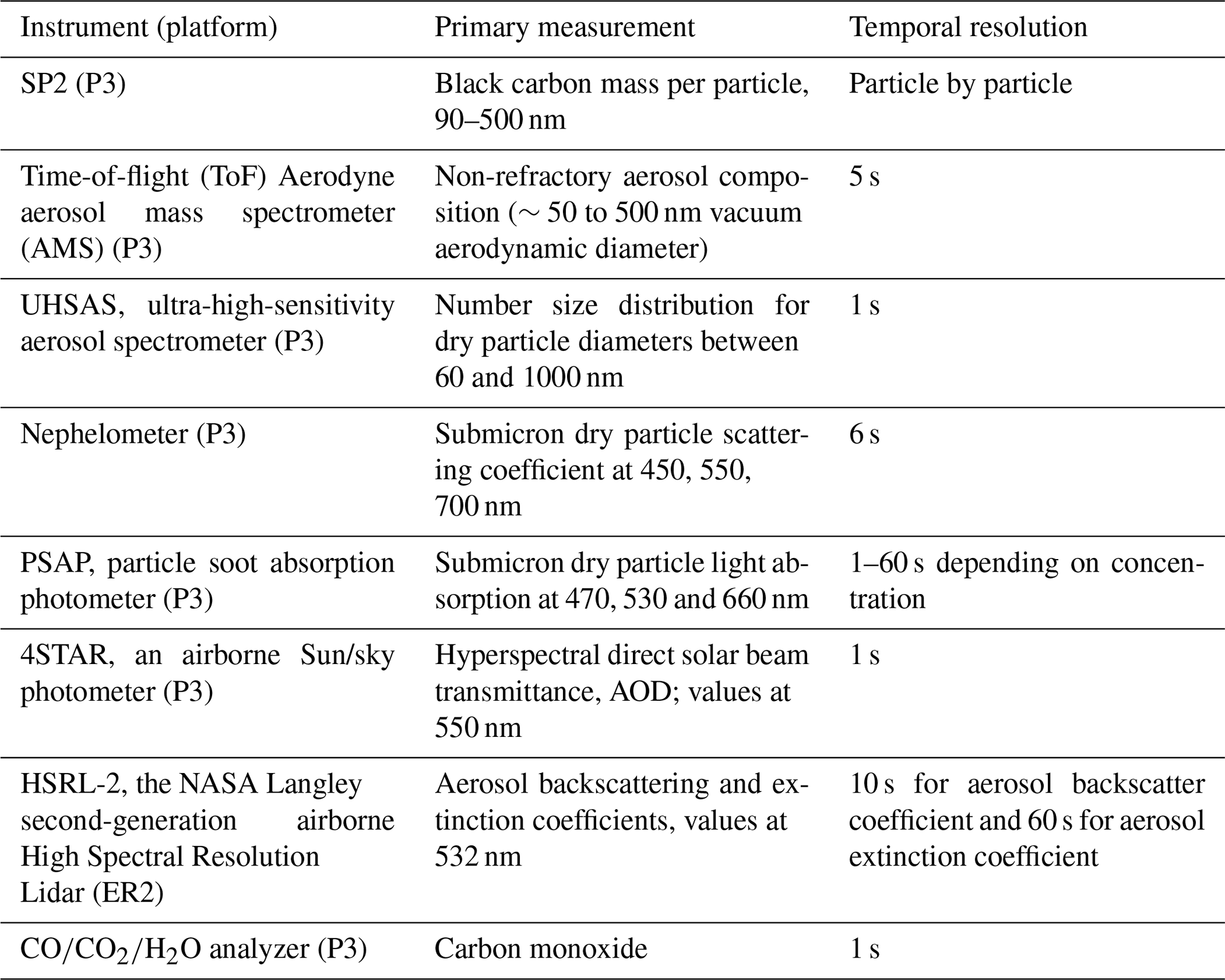
Figure 2 Observed vertical profiles of relative humidity, derived from the dew point measurements. The blue, orange, and green markers indicate the marine boundary layer (MBL), the lower FT, and mid-FT, respectively, as defined in the text. The gray markers indicate the data that do not belong to either group, with most of them in the inversion.

3 Framework for the model–observation comparison

3.1 Vertical ranges

The analysis is performed in three altitude ranges: 3–6 km, the region above the cloud top up to 3 km, and the cloud-topped marine boundary layer (MBL). During September 2016, within the sampled domains, the cloudy boundary layer is materially separated from the much drier FT by a strong temperature and moisture inversion, evident in aircraft RH profiles (Fig. 2). For the in situ observations available from the P3, we define the MBL as altitudes below (RH(%)–60) × 40 m.

For models, an alternative definition of the MBL top height was applied to facilitate future model–observation intercomparisons using ORACLES 2017 and 2018 aircraft data that include sampling from more equatorward regions of the southeastern Atlantic, where cloud cover is lower and clouds are more frequently multi-layered. The model MBL top is calculated as the level where the vertical derivative of the specific humidity with respect to altitude is a minimum. This defines the depth of the layer where the surface has a significant immediate influence on the moisture, which is often larger than the traditional “well-mixed” region where the potential temperature is nearly constant. First, we calculate dq∕dz, where q is specific humidity and z is altitude, at all grid points up to 3 km over oceanic regions and 6 km over land (small islands in the SE Atlantic, e.g., Saint Helena and Ascension, are considered oceanic). The different altitudes for land and ocean are chosen because (1) boundary layers on the African continent are often quite deep, up to 5–6 km (Chazette et al., 2019); and (2) occasionally the dq∕dz minimum over the oceans is at the top of the smoke layer, restricting the MBL depth to a maximum of 3 km (smoke layer tops are always higher). Next, we find the altitude where dq∕dz is a minimum. The two definitions of the cloud-topped MBL only differ slightly within the WRF-CAM5 model, with the RH-based definition placing the mean top of the MBL 120 m higher than the gradient-based one. Model data are only selected from the bottom half of the MBL to avoid potential cloud artifacts.

An altitude of 3 km is chosen to distinguish the lower and mid-FT in both observations and models. The lower FT is defined by the altitude range between cloud top or 500 m, whichever is higher, up to 3 km, with the additional requirement of ambient RH below 60 %. The lower FT contains aerosols that are more likely to mix into the MBL over the southeastern Atlantic at some time (Diamond et al., 2018; Zuidema et al., 2018). In contrast, the only interaction of the upper, 3–6 km layer with the underlying cloud deck in the short term is through radiation.

Figure 3 Left: the boxes selected for the model–observation comparison, overlaid on the P3 and ER2 flight paths (with HSRL-2 observations) from September 2016 and NASA's Blue Marble: Next Generation surface image, courtesy of NASA's Earth Observatory. Right: the altitude and longitude of the flights averaged over 60 s. The ER2 was at altitude of about 20 km except for take-off and landing.

3.2 Horizontal and temporal ranges

An additional challenge for any model evaluation using observations, especially in situ, is the scale mismatch. The in situ measurements are collected at spatial scales of approximately one sample per ∼100 m, one location at a time. In contrast, the model values represent averages over a horizontal grid spacing of tens of kilometers, available at regular intervals. The sampling bias is reduced by aggregating the data from both the observations and models into pre-defined latitude–longitude boxes (Fig. 3). Box-and-whisker plots summarize the full range of the distribution as the 10th, 25th, 50th (the median), 75th, and 90th percentiles as well as the means and standard deviations. This approach is similar to that applied within AEROCOM studies (Katich et al., 2018), but our data aggregation occurs within smaller domains and aims to capture regional spatial gradients, similar to Wyant et al. (2010, 2015). Observations are first averaged over 1 min intervals from their native values to limit the small-scale variability and instrument noise. A 1 min mean is equivalent to an approximate horizontal scale of 7–10 km at the typical P3 aircraft speed and 12 km at the typical ER2 speed.

One of the three main corridors encompasses the routine flight track, with individual grid boxes centered at 24^∘ S, 14^∘ E; 22^∘ S, 12^∘ E; 20^∘ S, 10^∘ E; 18^∘ S, 8^∘ E; 16^∘ S, 6^∘ E; 14^∘ S, 4^∘ E; 12^∘ S, 2^∘ E; and 10^∘ S, 0^∘ E, each having corners at 2^∘ north, east, south, and west, respectively, of the center. Another coastal north–south corridor has the southernmost grid box centered on 22^∘ S, spanning between 9 and 11.75^∘ E. Seven grid boxes are located every 2^∘ north of this, with the northernmost grid box centered on 8^∘ S. A third, west–east corridor covers the larger domain of the ER2 measurements, with individual grid boxes spanning latitudinally between 10 and 6^∘ S and separated longitudinally at 2^∘ intervals beginning at 3^∘ W to the west and 13^∘ E in the east. The box for Saint Helena island spans between 6.72 and 4.72^∘ W, between 16.93 and 14.93^∘ S.

All P3 and ER2 flights occurred during daytime, with data primarily gathered between 09:00 to 16:00 LT in central African time (07:00 to 14:00 UTC). The P3 sampled for 96 h in the diagonal and meridional corridors. The ER2 sampled for 30 h in these corridors and 8 h in the zonal corridor. The models are sampled at the 3-hourly times closest to those of the measurements, except for the climatology study presented in Sect. 4. Diurnal variations in aerosol properties are small and not considered. The number of samples contributing to each grid box, from both the observations and the models, is indicated on each comparison. Observational sampling is most sparse within the boundary layer, where there is also less aerosol, and at the northern end of the coastal corridor, for which comparisons contain too few samples to be truly representative.

4 Representativeness of the airborne sampling

An analysis based on MODIS clear-sky aerosol optical depths in the planning stage of the ORACLES mission indicated that the ORACLES sampling would be sufficient to capture the monthly mean. Our analysis based on WRF-CAM5 and GEOS-5 model output of aerosol extinctions confirms this. The daytime model outputs for the whole month of September occurring within the defined grid boxes are compared to the smaller data set of model output sampled closest in space (in the vertical and horizontal) and time to the observations.

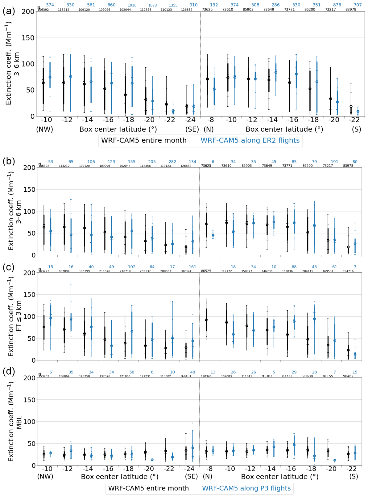
Figure 4 Extinction coefficients compared between two extracts (monthly climatology and flights) of WRF-CAM5 simulations. Panel (a) is along the ER2 tracks for altitudes between 3 and 6 km. The other three panels are for the P3 tracks for 3–6 km (b), the top of MBL to 3 km (c), and the MBL (d). In each panel, the abscissa represents the eight diagonally aligned boxes and eight meridionally aligned boxes described in Sect. 3.2 and Fig. 2. In each box, the bars indicate the monthly climatology (black) and samples along the flights (blue). Distributions are represented as box-and-whisker plots encompassing the 10, 25, 50, 75, and 90th percentiles, with circles indicating the mean and mean ± standard deviation values. The numbers in small print at the top of each panel indicate the number of samples.

The WRF-CAM5 model aerosol extinctions between 3 and 6 km altitudes corresponding to the days when the ER2-borne HSRL-2 extinction measurements are available (Fig. 4a, blue boxes and whiskers) generally agree well with the values based on the entire month (black boxes and whiskers). The same can be said for the comparison based on the P3 flight days (Fig. 4b), for both the diagonal and meridional corridors (left and right halves, respectively, of each panel). This conclusion is based on an evaluation of the mean bias (MB) and the root mean square deviations (RMSDs) for the two model populations. The MB between the monthly mean and flight-day-only means is between −10 % and +10 % of the monthly means. The RMSDs based on the model output from the flight days only are 20 %–30 % of the monthly mean values for each aircraft. The MB and RMSD values are provided in Table S1 in the Supplement for the two aircraft and three layers. Good agreement is also apparent within the MBL, if for much smaller extinctions (Fig. 4d). In the layer extending above the MBL up to 3 km (Fig. 4c), the P3 flights may have sampled more aerosol than was representative of the monthly mean, with the P3 flight-day extinction means exceeding the monthly means by approximately 20 % in many of the boxes. In-flight sampling decisions that routinely favor more smoky conditions may be responsible for some of the bias in the free troposphere. Comparisons in the free troposphere based on BC, organic aerosol (OA), CO, and ACAOD are mostly similar to those based on the light extinction. In the MBL, the mean BC and OA mass concentrations on flight days exceed the monthly mean values by approximately 30 %–40 % (Table S1 in the Supplement). The first P3 flight day, on 31 August 2016, documented more thoroughly in Diamond et al. (2018), sampled the most polluted boundary layer of the entire campaign and may be responsible for the noted bias in the boundary layer. Overall, the flight days capture the spatial trend well in the mid-troposphere and MBL, and somewhat less so in the lower FT especially near the coast.

Results from GEOS-5 (Table S1) are similar to those from WRF-CAM5. The only exception is in the lower FT (above MBL-3 km), where GEOS-5 shows that ORACLES flights along these corridors sampled lighter aerosol loading than the month-long average, by about 10 %, while WRF-CAM5 shows heavier smoke loads as mentioned above. In addition, GOES-5 places the smoke plume bottom heights within 100 m of its monthly mean, while WRF-CAM5 places them approximately 400 m higher (Table S1).

To summarize, the mean biases are generally between −10 % and +30 % in the lower FT and MBL, and less within the 3–6 km layer. To this extent, the ORACLES observations represent the regional climatology for September 2016.

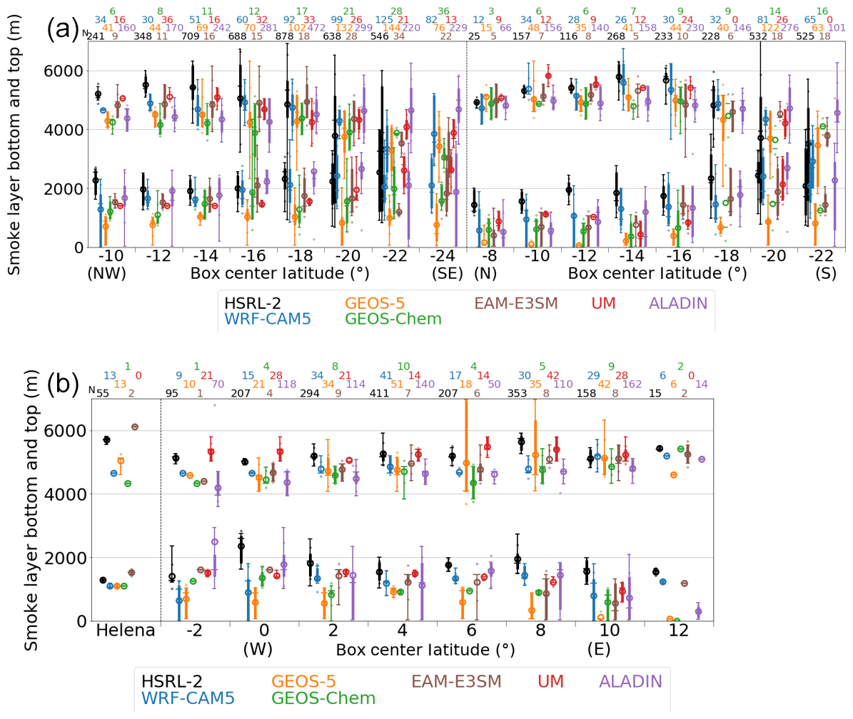
Figure 5 Smoke layer bottom and top altitudes. Smoke layers are identified through HSRL-2 backscatter intensities exceeding 0.25 Mm⁻¹ sr⁻¹, ALADIN extinction coefficient exceeding 17 Mm⁻¹ and, for other models, BC mass concentration exceeding 200 ng m⁻³; see Sect. 2.1 for details. Panel (a) is for the diagonal and meridional corridors, while (b) is for Saint Helena island and the zonal corridor; see Sect. 3.2 and Fig. 2. In each box, the bars indicate the observations from the ER2 aircraft (black) and model products (colors). See Fig. 4 for a description of each bar and number. The model values presented here are sampled along the longitude, latitude, and time of the flights. Missing box whiskers indicate products unavailable.

5 Evaluation of model aerosol plume heights

Here, we provide an evaluation of the free-tropospheric aerosol layer top and bottom altitudes, in preparation for the comparisons of the vertically resolved values. HSRL-2 observations generally show a better defined plume with larger aerosol loads in the mid-FT than in the lower FT, the latter often separated from the cloud top (Burton et al., 2018). The HSRL-2 observations indicate that the smoke layer top is highest, at around 5–6 km, between 9 and 17^∘ S (Fig. 5a). The mean aerosol bases are typically located at 1.5–2.5 km, rising slightly from north to south. The zonal gradient in observed plume top and bottom heights along 8^∘ S is small (Fig. 5b), with mean altitudes $+/-$ standard deviations between 3^∘ W and 13^∘ E of 5.25 km $+/-$ 180 m and 1.74 km $+/-$ 290 m, respectively.

All of the models tend to place the smoke plume at a lower altitude than the HSRL-2, especially in the northern half of the area. GEOS-5 and GEOS-Chem underestimate the mean top heights most severely, both by 500 m on average. The negative bias does not exceed 200 m for UM, EAM-E3SM, WRF-CAM5, and ALADIN-Climate (Fig. 5, Table S1). These biases are generally within the model vertical layer thickness at these altitudes (e.g., WRF-CAM5 has ∼500 m layer thickness at 5 km altitude) so that at least the <200 m underestimates are within the expected model uncertainty. The underestimates in the aerosol layer bottom heights are more diverse (300–1400 m) among the models. The mean bias is larger than for the top height for each of the models. A consequence is that all models generally overestimate the smoke plume geometric thickness. As with the top heights, the GEOS-Chem and GEOS-5 models underestimate the bottom altitudes most severely.

Despite generally placing the FT aerosol layers too low, most models are able to capture an equatorward increase in the aerosol layer tops and a poleward increase in the layer bases. Most models skillfully locate the maximum aerosol layer tops at 13–15^∘S, slightly south of the maximum outflow and close to the coast in the meridional corridor. One exception is ALADIN-Climate, which overall underestimates the top height by ∼500 m but overestimates it further to the south. As a result, while the bias is small, the variability between the grid boxes is somewhat greater for ALADIN-Climate (RMSD 800 m) than for WRF-CAM5 (400 m), UM (400 m), and EAM-E3SM (500 m), and is closer to that for GEOS-5 (600 m) and GEOS-Chem (800 m). The model variability is generally lower than the observed variability within the southernmost boxes. The observed smoke heights near 20^∘ S are more variable than further north, possibly related to stronger meteorological influences originating in the southern midlatitudes that models have a harder time capturing.

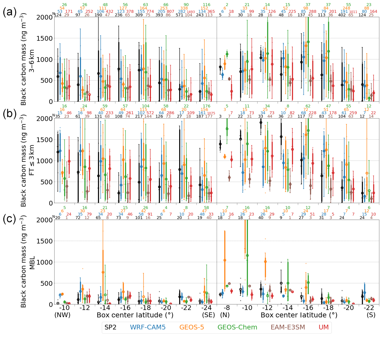
Figure 6 Black carbon mass concentrations compared between observations (black) and models (colors) for (a) 3–6 km, (b) the top of MBL to 3 km and (c) the MBL. The left-hand side of each panel corresponds to the eight diagonally aligned boxes of the routine flight path, and the right-hand side to the eight meridionally aligned ones described in Sect. 3.2 and Fig. 2. See Fig. 4 for a description of each bar and number.

6 Evaluation of models at bulk vertical levels

The six models are compared against the observations within the three pre-defined bulk vertical layers using box-and-whisker plots to capture the mean and the variability. Comparisons for the diagonal corridor are shown to the left of those for the meridional corridor in Figs. 6–16. The mean bias and standard deviations of each of the model products from the observations are summarized in Table S2 in the Supplement. The model products provided in this section are sampled near the space and time of the airborne measurements rather than monthly values.

6.1 Aerosol chemical and physical properties and carbon monoxide

Figure 6 compares the observed versus modeled BC mass concentrations at ambient temperature and pressure for the five models that report BC. Most models underestimate free-tropospheric BC on the diagonal corridor between 16^∘ S, 6^∘ E, and 10^∘ S, 0^∘ E. Near the coast, particularly in the lower free troposphere, the models tend to overestimate BC in the southern part of the domain, where less smoke is present, and underestimate BC in the northern part of the domain, although the model diversity is high towards the north. The strong increase in observed BC concentrations from south to north, consistent with northward decreases in the smoke layer bottom height (Fig. 5a), is not represented in most models. The WRF-CAM5 model (blue) agrees best with the SP2 observations (black), with an RMSD between the 16-grid-box means of 170 ng m⁻³ in the mid-FT (3–6 km altitude; Fig. 6a). The agreement of the GEOS-5 (orange) model with the measurements is slightly poorer, with an RMSD of 210 ng m⁻³. These values are around 30 % of the mean observed values, as noted in parentheses in Table S2. Little systematic bias is discernible in the figure. The MB of the WRF-CAM5 box means is as small as +10 % (Table S2).

In contrast, GEOS-Chem has almost no MB but an RMSD that is 50 % of the mean (Fig. 6, green) due to underestimates in the northern half of the diagonal corridor and overestimates closer to the coast. This shift is consistent with the increasing underestimate in the smoke top height as the plume advects towards the west in this model (Fig. 5). UM and EAM-E3SM underestimate BC mass concentrations in the 3–6 km layer with an MB of −40 % in all regions, with this systematic bias driving the RMSD.

The model–observation RMSD is greater in the lower FT than in the mid-FT for WRF-CAM5 (60 %), GEOS-5 (60 %), and EAM-E3SM (80 %). GEOS-Chem performs in this layer similar to its performance in the 3–6 km layer, with an RMSD of 50 % and no apparent bias. Underestimates are less severe in the UM model in this layer (−20 % MB) than at 3–6 km.

Much less BC is observed in the MBL (Fig. 6c) than in the FT, consistent with an elevated aerosol layer only slowly mixing into the boundary layer. Overall, the models place too much BC in the MBL further offshore and to the north. Individual model biases are not clearly correlated with those in the lower free troposphere. GEOS-5 overestimates MBL BC more significantly (+170 % MB) than in the FT (+10 %–20 %), as does GEOS-Chem. EAM-E3SM shows better agreement with observations in the MBL than above it. WRF-CAM5 and UM do not noticeably skew the BC vertical distribution towards the MBL. WRF-CAM5 overestimates BC in the northernmost boxes on the diagonal corridor but by less than GEOS-5.

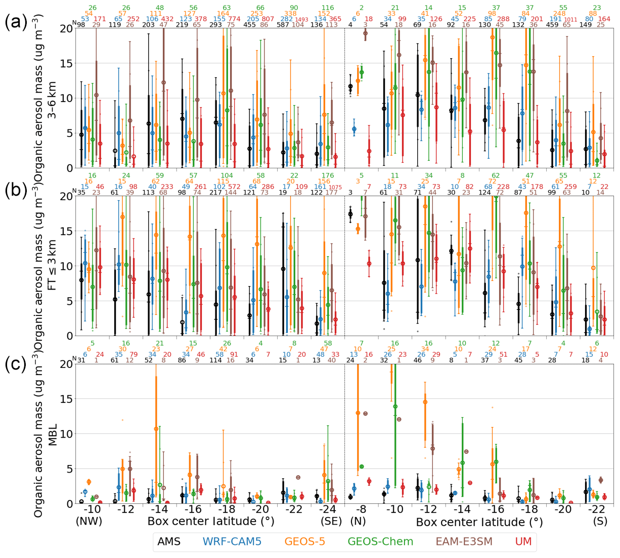
Figure 7 Same as Fig. 6 but for organic aerosol mass. The range of vertical axis is chosen for clarity. The GEOS-5 mean values in two boxes exceed the range.

Similarly to BC, measured organic aerosol (OA) mass concentrations at ambient temperature and pressure, shown in Fig. 7, increase from south to north near the coast, with concentrations lower further offshore. In contrast to BC, model OA values exceed those measured almost everywhere, with the exception of the remote 3–6 km layer. The models capture the south-to-north increase, with the greatest model diversity occurring to the north near the coast, but show somewhat greater deviations in OA than in BC. The RMSD in the 3–6 km layer, for example, is around 40 % for WRF-CAM5, 90 % for GEOS-5, 70 % for GEOS-Chem, 100 % for EAM-E3SM and 50 % for UM. In the lower FT, the GEOS-5 OA is more than twice that observed, and in the MBL more than 6 times that amount. Overall, the biases are more positive in the MBL than in the FT in all models. For both BC and OA, the RMSD is generally greater at lower altitudes.

Figure 8 Same as Fig. 6 but for carbon monoxide mixing ratio.

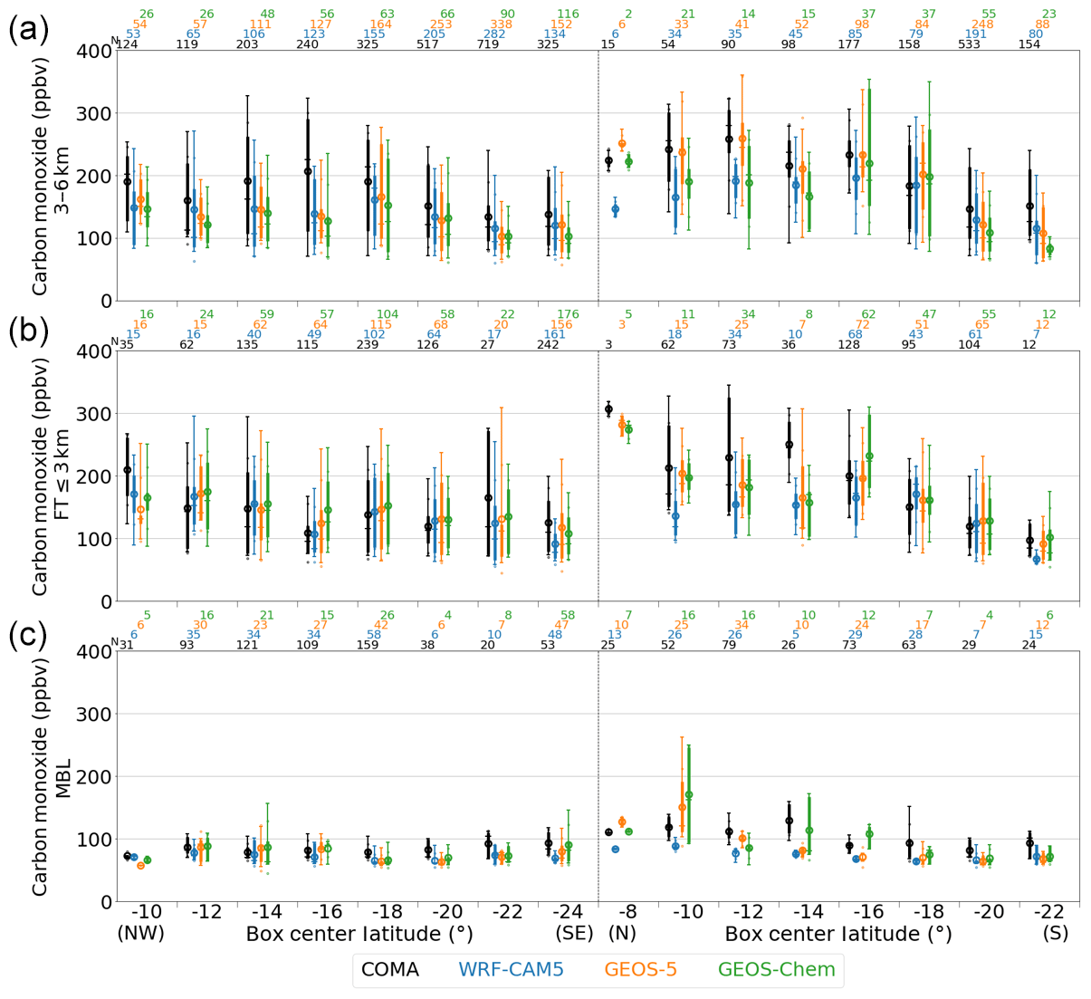
Only three models report a CO mixing ratio (WRF-CAM5, GEOS-5, and GEOS-Chem). The measured values range from 60 ppbv to over 500 ppbv (Fig. 8). The three models tend to underestimate CO, especially further offshore in 3–6 km and in the northern half of the near-coast corridor. WRF-CAM5 systematically underestimates CO by ∼20 % in the FT, as do GEOS-5 and GEOS-Chem to lesser degrees. In the MBL, where the observed mixing ratio is typically below 130 ppbv, the models are also typically biased low, most notably near the southern end and near the coast. GEOS-Chem shows an altitude dependence in the MB (−20 % in 3–6 km, −5 % below), but the dependence is not as strong as that seen in the carbonaceous mass concentrations. The relative RMSD, at 20 %–30 % for these models, is smaller than for any of the aerosol extensive properties. The relative model underestimates of CO further offshore are not as large as the relative underestimates of BC there. The relative model–observation CO deviations vary only mildly with altitude. This is strikingly different from the altitude dependence of the carbonaceous masses for GEOS-5 and GEOS-Chem. One uncertainty in the CO comparison, however, is that the background model values are not known. A higher background model value compared to that observed will have the effect of improving the comparison but for the wrong reason.

Figure 9 Same as Fig. 6 but for dry volumetric mean diameter. Samples with 550 nm dry extinctions less than 10 Mm⁻¹ are excluded.

Only two models (WRF-CAM5 and the UM) report an aerosol diameter. The diameter of the emitted aerosol is prescribed within these models and allowed to evolve thereafter. The measured volumetric mean dry aerosol diameters from the UHSAS are close to 200 nm, with little geographical or altitude variation. The UM volumetric mean diameter is greater than the observation by 30–40 nm in the FT. In the MBL, the UM–observation differences in diameter are smaller, especially on the diagonal corridor (NW–SE boxes); WRF-CAM5 volumetric mean aerosol diameters exceed measured values by 40–80 nm in the FT and by 90 nm in the MBL (Fig. 9). Note that the evaluation of the comparisons to the observations is somewhat compromised by significant undersizing by the UHSAS instrument. This effect was revealed when sampling size-selected particles behind a radial differential mobility analyzer for some dozen time periods during the 2018 campaign. The size distribution adjusted for this effect improves scattering closure with coincident nephelometer measurements. That said, the cause for the inter-model spread is worth discussing. It is the prescribed volumetric geometric mean diameter, which is 375 nm within WRF-CAM5 for the emitted accumulation-mode particles (the geometric standard deviation is 1.8), compared to the UM's 228 nm. Note the volume (arithmetic) mean diameter is smaller than the volume geometric mean diameter. Future simulations will use diameters closer to that representative of biomass-burning emissions.

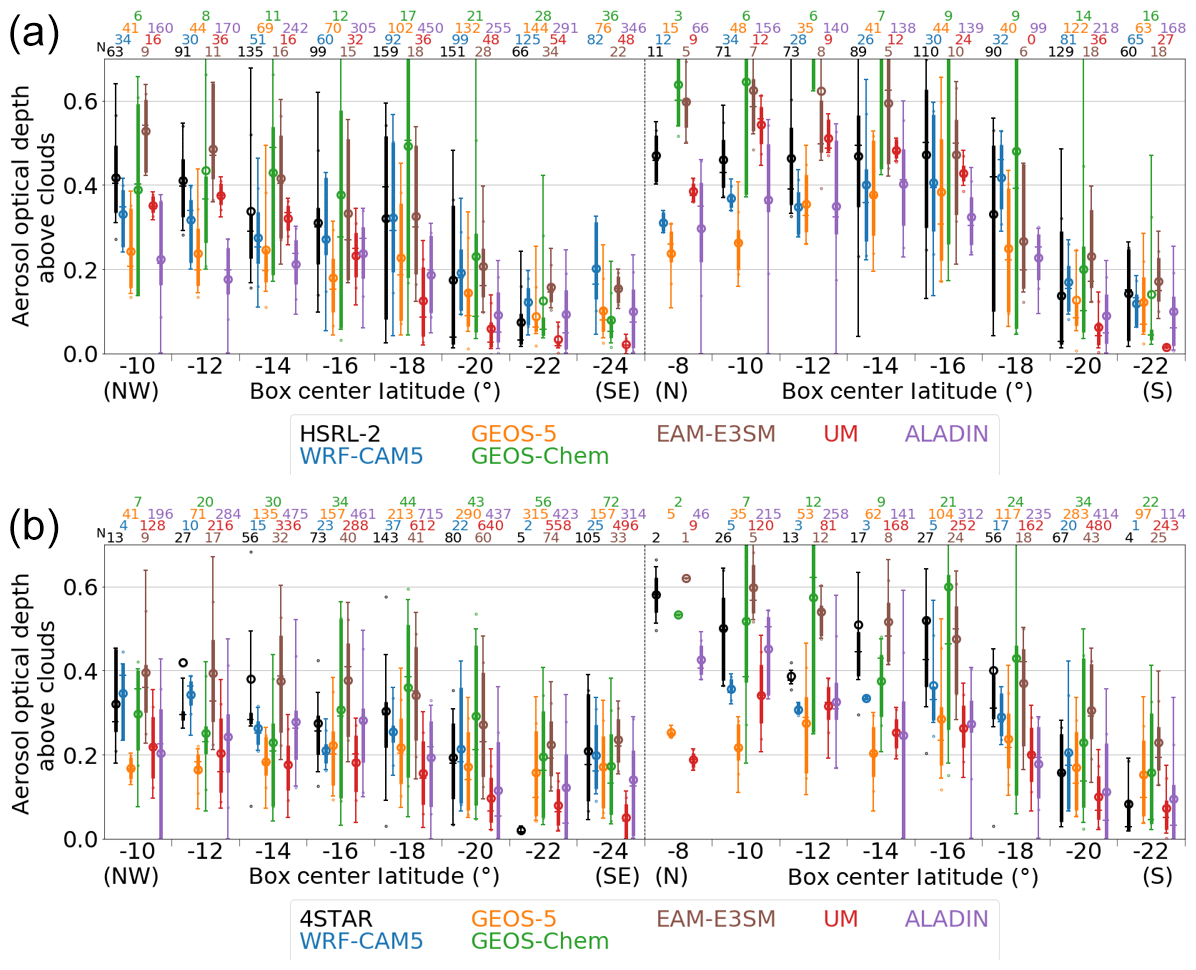
Figure 10 The aerosol optical depth above clouds (AC-AOD) compared between observations and models. Panel (a) compares to the HSRL-2 lidar observation from the ER2. Panel (b) compares to the 4STAR measurements made while the P3 aircraft was immediately above clouds.

6.2 Aerosol optical properties

The model-derived ACAOD are compared to observed mid-visible wavelength values from both the ER2-borne HSRL-2 lidar (Fig. 10a) and the P3-borne 4STAR Sun photometer (Fig. 10b). The two measurements indicate the same trends and approximately match each other over the routine flights but differ more near the coast, where the P3 values report higher ACAODs. This may reflect a sampling bias inherent to “flights of opportunity” targeting smokier conditions. The means of the model values match the measurements reasonably well but with significant differences between the individual models. The WRF-CAM5 values are biased low, by 10 %–20 % (Fig. 10, Table S2), particularly in the northern region closer to the plume core. Underestimates by GEOS-5 and ALADIN-Climate are larger still (∼30 %–40 %), and EAM-E3SM overestimates by 20 %. While these models show similar degrees of deviations for the two instruments, GEOS-Chem overestimates by 40 % relative to the HSRL-2 but only by 5 % relative to 4STAR.

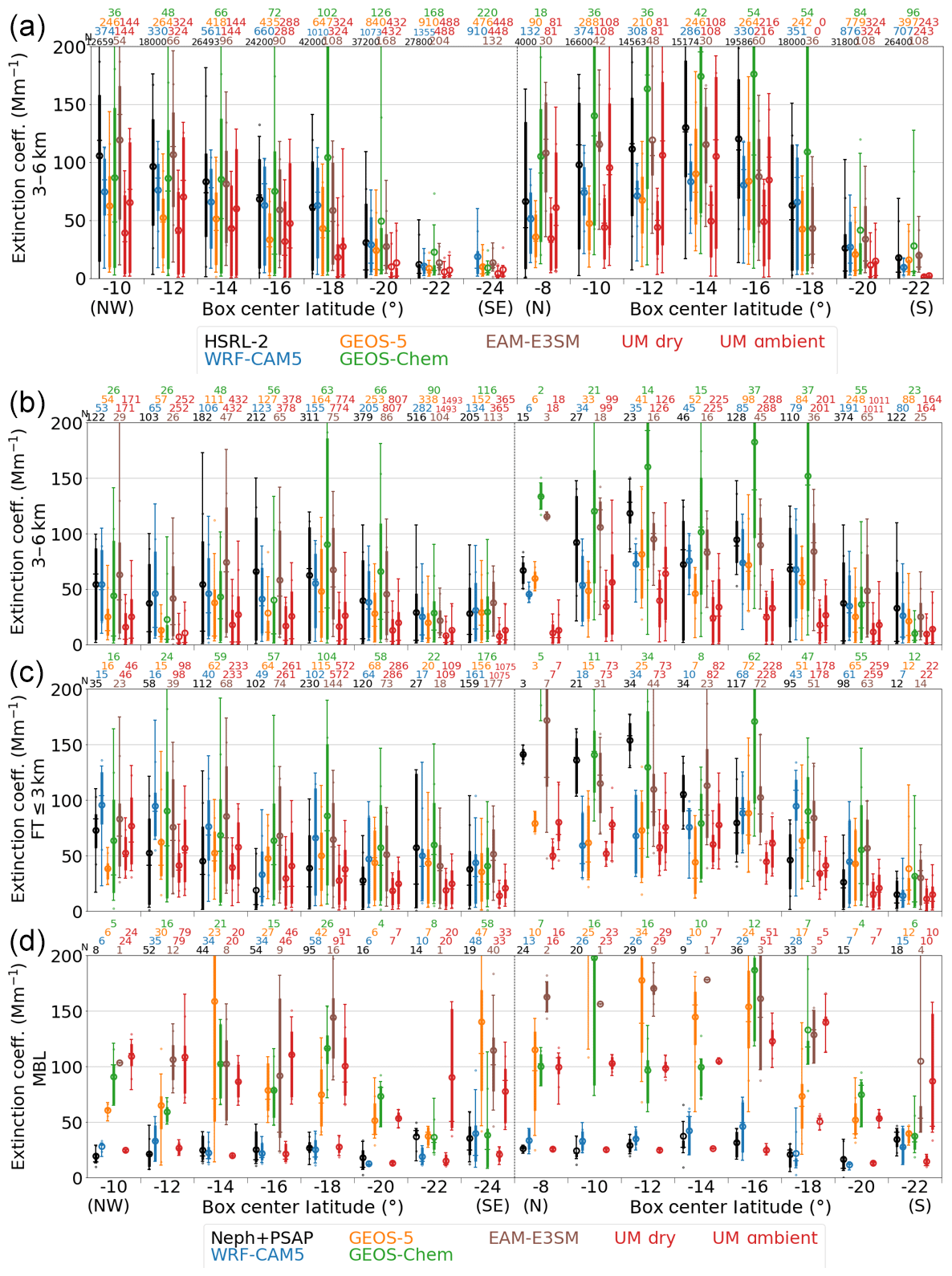
Figure 11 Extinction coefficients compared between observations and models. Panel (a) compares to the HSRL-2 lidar observation of the ambient particles from the ER2 for 3–6 km. The other three panels compare to the nephelometer and PSAP measurements of dried particles aboard the P3 aircraft for (b) 3–6 km, (c) the top of MBL to 3 km, and (d) MBL. For UM, the values for dry RH conditions are given to the left of the ambient ones.

The extinction measurements are based on two sources. The lidar extinction at ambient RH within the 3–6 km layer is shown in Fig. 11a. Measurements shown in the lower three panels of Fig. 11 are based on the sum of nephelometer scattering and PSAP absorption coefficients measured at low (∼20 %) RH. Note that the observed extinction in the MBL may be lower than true values for two reasons. First, since the relative humidity typically exceeds 85 % and the aerosols are more hygroscopic, the effect of aerosol hygroscopic swelling on the extinction is pronounced, with the ambient–RH∕dry ratio of light scattering exceeding 2.2 for half of our measurements when the dry scattering exceeds 1 Mm⁻¹. This estimate is based on concurrent, once-per-second measurements from two nephelometers, one set to a high RH (∼80 %) and the other to a low (∼20 %) RH value. In the FT, the ambient–RH∕dry ratio is estimated to be less than 1.2 for 90 % of the time. Second, the movement of the coarser particles through the inlet and tubing to the instruments in the aircraft cabin is limited. The inlet's size cut of approximately 5 µm is sufficient to measure nearly all scattering in the FT but likely not in the MBL, particularly at high wind speeds when there is likely to be a significant amount of coarse aerosol (McNaughton et al., 2007).

For both comparisons, the model extinction values refer to ambient RH, except for the UM model, for which extinction values are available at both ambient and dry RH. Model differences from the observations in the FT (Fig. 11) broadly follow those for ACAOD, meaning that the mean of the model values underestimates or overestimates the measurements offshore, particularly in the 3–6 km layer, and compares better to the south where less aerosol is present. Model diversity again is most pronounced to the north, near the coast. The ambient extinction modeled with WRF-CAM5 is lower than the HSRL-2 ambient extinction and the dry in situ extinction, both by 20 %. GEOS-5 underestimates the FT extinction to a greater degree than does WRF-CAM5, by 30 %–40 %. GEOS-Chem, in contrast to GEOS-5, has a positive bias in the FT (by +30 %–40 %). EAM-E3SM indicates smaller overestimates (0 %–20 %) in the FT, with values in the northern half of the near-coast corridor particularly close to the observation. UM generally underestimates the extinction in the free troposphere, by 30 % compared to the lidar extinction at ambient relative humidity and by 50 %–70 % compared to the low-RH in situ extinction.

Most models except for WRF-CAM5 and UM-dry appear to overestimate extinction within the MBL, with model biases almost reaching an order of magnitude in places. The gross overestimation within the MBL may reflect the instrument limitations, although GEOS-5 sea salt mass concentrations are known to be overestimated (Bian et al., 2019; Kramer et al., 2020). Without further information on coarse-mode boundary layer aerosols such as from sea salt, it is difficult to attribute extinction biases within the MBL directly to BBA, with comparisons against BC and OA being more informative when enough samples are available.

Figure 12 Same as Fig. 6 but for the scattering Ångström exponent.

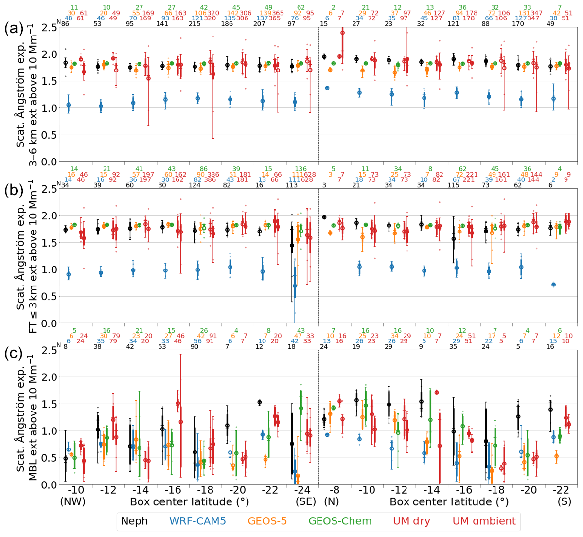
The scattering Ångström exponent is an independent if indirect measure of particle size that is more readily available from the models included here than is the aerosol size itself (Fig. 12). The Ångström exponent is computed as the slope of a linear fit of the scattering versus wavelength on logarithmic scales for cases where the 550 nm extinction exceeds 10 Mm⁻¹. Large scattering Ångström exponents tend to correspond to smaller particle sizes. Most models report scattering Ångström exponents in the free troposphere that are close to the observed values of 1.8–2.0, with an RMSD of 0.1 (Fig. 12). The scattering Ångström exponent is only systematically underestimated by WRF-CAM5, by an absolute value of 0.6–0.8, qualitatively consistent with the overestimated aerosol mean sizes (Fig. 9). The largest deviations are found in the northern end of the near-coast flights where the observations are relatively sparse. Within the MBL, all of the models tend to underestimate the scattering Ångström exponent, indicating that modeled particle sizes are larger than those observed behind the inlet and tubing under dry conditions. This model–observation discrepancy may also reflect an instrument limitation.

Figure 13 Same as Fig. 6 but for the absorption Ångström exponent.

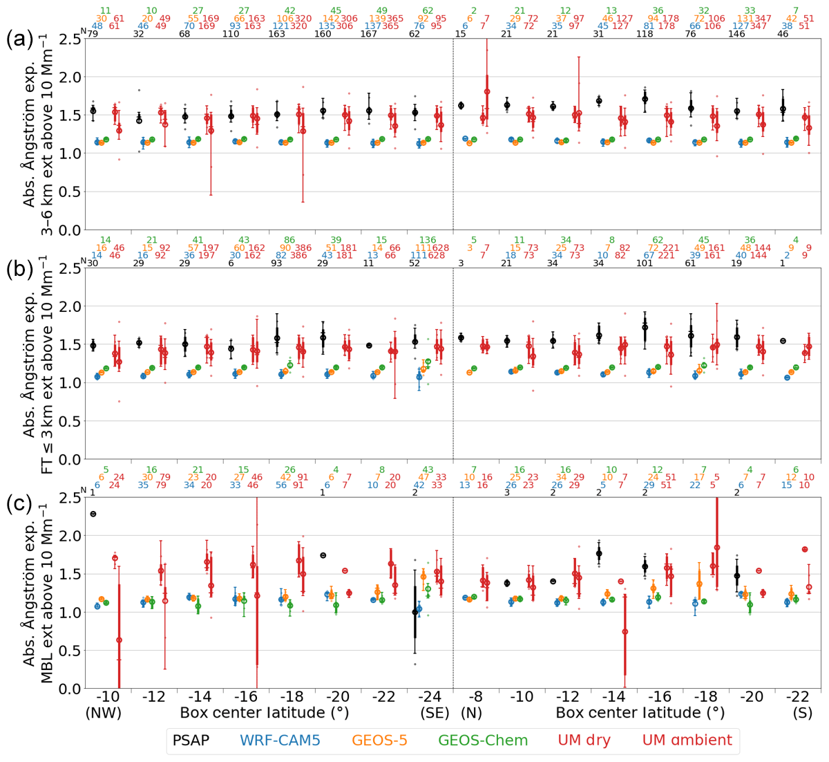
The absorption Ångström exponent differs from the scattering Ångström exponent in that it is a strong function of particle composition and secondarily of particle size. The observed absorption Ångström exponent typically ranges between 1.5 and 1.7 in the free troposphere. In contrast to the scattering Ångström exponent, the absorption Ångström exponent in the FT is systematically underestimated, by 0.1 for the UM dry aerosols, and by 0.4–0.5 in WRF-CAM5, GEOS-5 and GEOS-Chem (Fig. 13). The models have very small ranges in the absorption Ångström exponent, both within each of the comparison boxes and across them. Flatter modeled spectra would typically suggest model overestimates in BC absorption or underestimates in absorbing organic material. This inference is at first glance contradicted by the model comparisons to BC and OA mass concentrations. Further model evaluation of the model refractive indices is beyond the scope of this study, and deductions of appropriate values from the measurements remain a topic of ongoing research (Chylek et al., 2019; Taylor et al., 2020). The HSRL-2 aerosol typing algorithm, based on Sugimoto et al. (2006), did not indicate contributions from dust to the extinction of more than 5 %–10% on most flights, so that dust can be discounted as a significant influence on the observed absorption Ångström exponents. The model contributions from dust to the various optical parameters are not known, however.

Figure 14 Same as Fig. 6 but for SSA. Note that the modeled SSA refers to the ambient humidity, whereas the observations are for dried particles.

The single-scattering albedo (SSA) is key to establishing the radiative impact of the aerosol layer. Model values vary significantly (Fig. 14). All of the models, with the exception of UM, only calculate SSA at ambient relative humidity, whereas the observations are for dry aerosol only. Absorption by smoke as a function of RH is typically thought to be small, and most models assume that any RH influence on absorption can be neglected. As discussed previously, the impact of RH on scattering within the free troposphere is estimated to be within a factor of 1.2. This corresponds to an increase in SSA due to RH of at most 0.02. Comparison between ambient and dry SSA measurements finds smaller differences (Pistone et al., 2019), consistent with more sophisticated aerosol closure calculations (Redemann et al., 2001). The dry in situ observations indicate mid-visible SSA values of 0.86 to 0.89 in the mid-FT and slightly lower values in the lower FT, ranging from 0.81 further offshore, increasing to 0.86 near the southern end of the routine flights, to 0.87 closest to the coastal north. This vertical structure in measured SSA is also apparent in Redemann et al. (2020), with Pistone et al. (2019) discussing the full range of ORACLES SSA values.

SSA in the lower FT (Fig. 14b) is simulated well by WRF-CAM5 and GEOS-5, with minor biases (−0.01 or smaller in magnitude) and RMSD of 0.01–0.02. In the mid-FT (Fig. 14a), WRF-CAM5 systematically underestimates SSA by 0.03. GEOS-5 also underestimates the 3–6 km layer-mean SSA but by noticeably smaller margins near the coast. GEOS-Chem overestimates SSA most severely, by 0.06–0.07 in both FT layers. EAM-E3SM also overestimates by 0.06 in the lower FT and by 0.02 in the mid-FT. With the UM, while the ambient simulated SSA agrees reasonably well with the dry observations, the SSA for dried particles is underestimated by 0.07 in the mid-FT and 0.04 in the lower FT. UM uses hygroscopic growth factors for aged organics corresponding to 65 % of sulfate by moles (Mann et al., 2010), which is in the higher range for what is generally assumed for organics. Thus, the large differences between dry and ambient conditions shown by this model are likely not applicable for models that use low hygroscopic growth factors for organics.

Overall, there is large model diversity for SSA in the free troposphere, and no model can accurately predict SSA for the lower and upper layers, and as a function of distance from the coast. The models generally overestimate SSA in the MBL (Fig. 14c), though this assessment is subject to particularly poor statistics due to the scarcity of cases with dry extinction exceeding 10 Mm⁻¹, the lack of adjustment for the humidity effect and the loss of coarse particles prior to the in situ calculation.

7 Discussion

7.1 Differences between the models and observations for specific parameters

The six models in this study have several common features, most notably the underestimate of the smoke bottom height, and, to a lesser extent, the smoke top height. These biases are most apparent away from the coast. Model comparisons to the lidar-derived ACAOD indicate modeled ACAODs that are either biased high (EAM-E3SM) or low (GEOS-5, ALADIN-Climate), with WRF-CAM5 and UM comparing more favorably. Also, inter-model ACAOD differences are pronounced at the northern end of the coastal corridor. The models are most likely to underestimate the mean BC loadings further offshore and in the upper troposphere, and most likely to overestimate the values near the coast, in the southern part of the domain, in the lower free troposphere. The inter-model spread about the observations is largest to the north, close to the coast.

Some qualitative correspondence is apparent between the individual model BC biases and the aerosol emission databases used to initialize the models. Models based on the Quick Fire Emissions Dataset (QFED) emissions (WRF-CAM5, GEOS-5, GEOS-Chem) and Fire Energetics and Emissions Research (FEER) database (UM) produce BC mass concentration estimates within the free troposphere that are closer to the measurements than the EAM-E3SM model, which is based on the GFED emissions database. The QFED and FEER emission data sets provide larger biomass-burning emissions in the central African region compared to the GFED emissions source used by EAM-E3SM and ALADIN-Climate (Pan et al., 2020). Both QFED and FEER base their estimates on satellite-derived fire radiative power and aerosol optical depth, for which a remaining error may be the insensitivity of satellite retrievals to very small fires (Fornacca et al., 2017; Petrenko et al., 2017; Zhu et al., 2017). The GFED emissions estimate is based on satellite burned-area data and does not include any aerosol optical depth constraints. In EAM-E3SM, the monthly biomass-burning emissions are based on the GFED monthly mean for 1997–2000. Redemann et al. (2020) indicate that the aerosol optical depth over the southeast Atlantic in September 2016 was below a longer-term mean, implying that the offshore underestimate in EAM-E3SM BC mass is not explained by the use of a long-term monthly mean.

In comparison to BC, the model OA values are more likely to be overestimated relative to the measurements. The model OA values also in general show larger deviations from the measurements compared to BC, at all vertical levels. For organic aerosols, factors other than emission database can explain the model biases. While BC is generally treated as inert, OA undergoes chemical reactions whose representation is highly uncertain in models, especially for BBA. Most of the models within this study include some treatment of secondary organic aerosol (SOA), but the treatment is typically simple (Liu et al., 2012) and does not account for multi-day aging processes (Liu et al., 2016; Wang et al., 2020). An inaccurate or inadequate treatment of SOA could be a factor contributing to the generally poorer representation of OA versus BC in the models. The discrepancies between BC and OA model skill become even larger in the MBL, where insufficient wet removal in the model MBL due to assumptions on hygroscopicity of organic aerosol (Kacarab et al., 2020) may be an additional factor.

The extinction coefficients in the FT and ACAOD within GEOS-5 and WRF-CAM5 are underestimated, even though the aerosol mass is generally overestimated. This is partly because some aerosol components (primarily nitrate and ammonium) are not incorporated into the models. WRF-CAM5, for example, does not compute nitrate and ammonium, which contribute 9 % and 5 %, respectively, to the aerosol mass as observed with the AMS and SP2. These missing aerosol mass components are too small to fully account for the extinction underestimates by 20 %–40 %, however. Sampling measurement bias is unlikely to fully explain the discrepancy either, because the modeled extinction is also underestimated by greater than 10 % against the HSRL-2 observations, which benefit from their ability to sample the full vertical column. We therefore conclude that the mass extinction efficiency (MEE) implicit in these models must be underestimated.

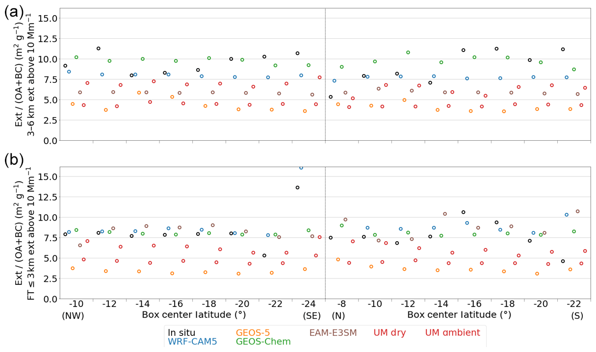
Figure 15 The ratio of extinction to the sum of organic aerosol and black carbon masses, computed for box mean values. The in situ observation of extinction is for dried particles, while the models refer to ambient humidity conditions except for UM dry. Panels (a, b) are for 3–6 km and for the top of boundary layer to 3 km, respectively.

While the missing mass components prevent us from computing MEE in the models, the ratio of extinction to carbonaceous masses (OA + BC) can illustrate its spatial and inter-model variabilities in an approximate manner, provided that biomass-burning particles dominate the aerosol mass and extinction (which is the case in the biomass-burning plume in the FT). The quasi-MEE calculated from the box mean ambient extinction and masses in the FT is shown in Fig. 15. The observed value is approximately 8 m² g⁻¹ in most boxes, or slightly greater. Each model takes a fairly constant value across the locations, while the observations indicate more spatial variability. In the lower FT, the WRF-CAM5, GEOS-Chem, and EAM-E3SM values are also near 8 m² g⁻¹. The UM ambient quasi-MEE is lower at about 6 m² g⁻¹. For the 3–6 km layer, the modeled quasi-MEE values are more diverse. WRF-CAM5 and GEOS-Chem values remain within 8–10 m² g⁻¹, while both EAM-E3SM and the UM ambient values are closer to 6 m² g⁻¹. GEOS-5 underestimates the quasi-MEE most severely in both layers. Any model underestimates will be more pronounced when humidification of the measured values is taken into consideration, although the aerosol swelling from moisture within the FT contributes 20 % or less to the measured extinction. In contrast, UM, which provides both dry and ambient extinction, models a humidification upon the quasi-MEE of around 50 % (compare UM dry and UM ambient in Fig. 15).

The FT SSAs differ significantly between the models, from mean values of 0.92 (GEOS-Chem), 0.90 (EAM-E3SM), 0.84 (GEOS-5), 0.84 (WRF-CAM5), 0.80 (UM dry), and 0.85 (UM ambient), compared to observed values closer to a mean value 0.86 (Fig. 14). The significant overestimate of SSA by EAM-E3SM in the lower FT is coupled with overall weak emissions of absorbing smoke particles in this model. Models with higher SSA values tend to possess larger ratios of the extinction to the sum of the BC and OA aerosol mass concentrations, termed “quasi-MEE”. It is unlikely that observational limitations are large enough to explain the model–observation discrepancies in quasi-MEE. Mie calculations for common ranges of refractive index and density conclude that the MEE for the observed UHSAS size distributions cannot be much smaller than 4 m² g⁻¹; the quasi-MEE, missing some aerosol mass components, should be greater than this. The underestimates by some of the models are difficult to reconcile with their Ångström exponents. For example, an overestimated volumetric mean diameter of around 300 nm (UM and WRF-CAM5), combined with an underestimated scattering Ångström exponent (WRF-CAM5), should be consistent with an overestimated quasi-MEE, but it is not. Relative humidity contributions to the SSA and quasi-MEE are estimated to be less than 0.02 and 20 %, respectively. A satisfactory evaluation of aerosol size and its impact on optical properties was not possible with the available model output. Aerosol size was only available from two models, both of which use prescribed diameters that are too large. A full absorption closure for both the measurements and models is beyond the scope of this study. These results do reveal the difficulty in representing both aerosol extinction and mass correctly. The model representation of aerosol mixing states, sizes, and refractive indexes, as well as ambient RH, all contribute to model–observation differences in SSA and the quasi-MEE. We recommend an assessment of other models using the ORACLES observations, not just in terms of the individual properties but also the relationships between them.

7.2 Potential causes for discrepancies between the models and observations

Some of the model–observation disagreement can be attributed to poor counting statistics. This is apparent, for example, within the near-coast boxes at 8^∘ S in the lower FT, for which only 4–5 min of in situ data are available. Other observations are not continuously available during flights, for example, ACAOD from 4STAR, for which the aircraft needed to be located above clouds and below the entire plume extent. Nevertheless, these data are particularly valuable because they indicate that flight-planning choices led to the P3 preferentially sampling higher aerosol loadings close to the coast, compared to the HSRL-2 upon the ER2.

Other variability can be attributed to model specifications. GEOS-Chem generally exhibits greater variability, both within boxes and across them, than does WRF-CAM5, notably in ACAOD (Fig. 10). Since these two models employ the same daily emission scheme and both allocate it to daytime burning in similar manners, the difference in the variability must be due to a combination of other model aerosol processes, driving meteorology (NCEP for WRF-CAM5 versus GEOS-FP for GEOS-Chem), and model resolution. Although the domain size invoked for the regional models could have the effect of eliminating some biomass-burning sources (James Haywood, personal communication), the domains for both regional models, WRF-CAM5 and ALADIN-Climate, encompass all of the burning regions of Africa for the time period of September 2016.

The smoke layer bases are determined using a black carbon mass concentration threshold, and the model that places the aerosol layer the lowest (GEOS-5), also overestimates the aerosol mass concentration (both BC and OA) within the boundary layer the most. This suggests GEOS-5 model likely over-entrains into the boundary layer, behavior that is in part encouraged by a low-level cloud fraction that is too small (not shown), reducing the inversion strength. WRF-CAM5, which has the aerosol base altitude close to the observations, has the smallest overestimate of aerosol mass within the boundary layer.

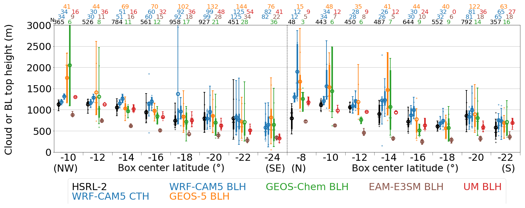
Figure 16 Cloud top heights (CTHs) as measured by the HSRL-2 and depicted by WRF-CAM5, and boundary layer heights (BLHs) from WRF-CAM5, GEOS-5, GEOS-Chem, EAM-E3SM, and UM. Cloud top heights are limited to 4 km to exclude mid-level clouds.

The low bias of the smoke layer heights has previously been attributed to an overestimate of subsidence over the ocean (Das et al., 2017), an underestimate in the smoke injection heights at the source (Myhre et al., 2003), and the dry deposition velocity scale factor (Regayre et al., 2018). Of these, an exaggerated subsidence over the ocean would not only influence the transport of smoke but also the top height of clouds. Often the smoke base height is determined by the cloud top height in models, as smoke concentrations in the MBL are usually below the threshold used for defining the smoke boundaries. However, as is made clear by a comparison of the model cloud top heights to those observed (Fig. 16), the model cloud top heights are typically higher than those observed, except for the EAM-E3SM model. Note that mid-level clouds (Adebiyi et al., 2020) are excluded by only selecting for cloud top heights less than 4 km. The overestimated model cloud top heights are particularly noticeable to the north, near the coast. An exaggerated model subsidence can also not fully explain model underestimates in the smoke layer base altitude that are as large as 1400 m.

Overall, a model which places the aerosol layer base too low, and the cloud top too high, has the potential to overestimate BBA entrainment into the MBL. However, the placement of a model plume that is lower than observations but for which the model is still able to properly represent MBL concentrations, is likely indicative of compensating model biases that will require further exploration.

7.3 Impact of model biases upon calculated aerosol radiative effects

The ultimate goal of this study is to provide groundwork towards improving the physically based depiction of the modeled aerosol radiative effects (direct, indirect, and semi-direct) for this climatically important region. Zuidema et al. (2016) indicate a wide range of modeled direct aerosol radiative effect (DARE) values for 16 global models. Similar to this study, no standardization was imposed upon the model simulations. Of these, the GEOS-Chem model is also represented within this intercomparison, with the caveat that some model specifications may have evolved in ways we are not aware of. The CAM5 model is also incorporated within the WRF-CAM5 regional simulation of the current study, using the same MAM3 aerosol microphysics. GEOS-Chem reports a small but positive August–September DARE (+0.06 W m⁻²), and the global CAM5.1 model reports the most warming (+1.62 W m⁻²) of the 16 models shown in Zuidema et al. (2016).

The current study does not assess the model cloud representations other than WRF-CAM5 cloud top height, upon which all the aerosol radiative effects also depend. Most models, including GOES-Chem, WRF-CAM5, and ALADIN-Climate, share the bias of generally underestimated BC mass within the 3–6 km layer offshore and overestimates closer to the coast. Although speculative, the weakly positive DARE within GEOS-Chem is consistent with a GEOS-Chem overestimate in ACAOD that is compensated by its SSA overestimate, all else equal. The EAM-E3SM model biases are similar and suggest similarly compensatory behavior will impact the model DARE estimates. The more robust performance of WRF-CAM5 within this intercomparison, if that can be extrapolated to the global CAM5, would imply support for the more strongly positive global CAM5 DARE estimate relative to the other models within Zuidema et al. (2016).

ALADIN-Climate is a regional model reporting a more positive top-of-atmosphere DARE of approximately 6 W m⁻² over the ORACLES domain for September 2016 (Mallet et al., 2019) than any of the global models. Reasons for this are beyond the scope of this study, but the ALADIN-Climate underestimate of ACAOD combined with a slight SSA overestimate suggest that the ALADIN-Climate DARE is likely still underestimated. Mallet et al. (2020) investigated the model sensitivity to smoke SSA and found a variation of 2.3 W m⁻² that can be attributed solely to SSA variability for July–September DARE. The UM uses a two-moment aerosol microphysics scheme that is updated from the one applied within the HadGEM2 model of de Graaf et al. (2014), and no UM DARE estimates are yet available. The EAM-E3SM incorporates a sophisticated new MAM4 aerosol scheme that explicitly includes the condensation of freshly emitted gases upon black carbon. The EAM-E3SM results within this study use a long-term monthly mean emission database, and future work will examine model DARE values specific to September 2016. An upcoming companion paper will include all of the variables needed to calculate DARE, allowing for a more quantitative evolution of the model bias propagation.

8 Summary

Six representations of biomass-burning smoke from a range of leading regional and global aerosol models are compared against 130 h of airborne observations made over the southeast Atlantic during the NASA ORACLES September 2016 deployment. The comparison framework first aggregates the sparse airborne observations into approximately 2^∘ grid boxes and into three vertical layers: the cloud-topped marine boundary layer, the cloud top to 3 km, and the 3–6 km layer. The BBA layer is defined using BC within most of the models and comparable values of in situ backscatter for the lidar. The spatially extensive biomass-burning aerosol is primarily located in the FT. The WRF-CAM5 and GEOS-5 models establish that the measurements from the 15 flight days are representative of the monthly mean, with aerosol loadings averaged over the flight days generally between −10 % and +30 % of the regional September average. A strength of the comparison is its focus on the spatial distribution of the aerosol, and it is a more detailed assessment of a wider range of aerosol composition and optical properties than has been done previously.

All six models underestimate the smoke layer height, thereby placing the aerosol layer too close to the underlying cloud deck. GEOS-5 and GEOS-Chem underestimate the smoke layer base to the greatest degree, by 1400 and 900 m, respectively. Despite the overestimated aerosol layer thicknesses, most models underestimate the ACAOD offshore in the diagonal corridor. A spatial pattern emerges in which the models do not transport enough smoke away from the coast, so that many smoke layer properties (aerosol optical depth, smoke layer altitudes, BC mass concentrations, and CO) are underestimated offshore, particularly in the upper FT, and overestimated closer to the coast, particularly towards the south where less aerosol was observed. An exception is the OA mass concentration, for which the models typically estimate higher amounts than they do of BC.

The relationship of the aerosol optical properties to their composition is investigated. Some modeled aerosol extinction in the FT is typically too low. Within the boundary layer, the modeled extinctions typically exceed observed values, but undersampling of the coarse-mode aerosol by the aerosol instrument inlet also calls into question the measured values within the boundary layer. The modeled ratio of the extinction to the sum of the BC and OA mass concentrations is often too low, with too little spatial variability, and with significant inter-model differences. Modeled absorption Ångström exponents are typically too low. The FT SSA ranges widely across the models, with mean model values ranging between 0.80 and 0.92; in situ values are approximately 0.86. Higher SSA values correspond with higher ratios of the extinction to the sum of the BC and OA mass concentrations. Overall, these comparisons indicate challenges in representing the more complex OA formation and removal processes in climate models, and suggest that a realistic model representation of the OA may be critical for the accurate modeling of aerosol absorption. A similar conclusion is reached within Mann et al. (2014) but emphasizing the importance of organic aerosol representation for particle size distributions.

Most models captured the observed CO measurements more accurately than the BC mass concentration, although lack of knowledge of model CO background levels cautions against too much interpretation. That said, modified combustion efficiency calculations based on measurements are more consistent with flaming-phase combustion (Wu et al., 2020). Such burning conditions tend to favor BC emission over that of CO and OA (Christian et al., 2003). Further interpretation of the relationship between the modeled BC and OA mass concentrations and CO mixing ratios requires an assessment of the emission source functions and organic aerosol processes within each model that is beyond the scope of this study. OA typically dominates the composition of biomass-burning emissions (Andreae, 2019) and is subjected to a myriad of further processes, with the processes dominating long-range transport still under scrutiny (Taylor et al., 2020; Wu et al., 2020). Thus, it is not surprising that the model–observation comparisons of the OA mass concentration are arguably the most variable of the different properties assessed. The formation and/or evaporation of SOA is a complex process known to not be well represented in models (Hodzic et al., 2020) but dominating the aerosol mass in the southeast Atlantic (SEA). The SEA is particularly challenging as the new measurements indicate that the mass proportion of OA to BC in highly aged biomass-burning aerosol is likely lower than for other regions of the world (Wu et al., 2020). EAM-E3SM has a relatively sophisticated aerosol treatment that explicitly considers aging but only as a condensation of H₂SO₄ and organic gases upon fresh BC and primary OA, thereby increasing the coating thickness. An evaluation of the EAM-E3SM aerosol optical depths has revealed that the modeled SOA condensation rates need to be scaled back over Africa to achieve agreement (Wang et al., 2020), indicating other aging processes are also likely occurring.

This comparison has focused on September 2016, when most of the BBA is located in the free troposphere. Free-tropospheric BC mass concentrations reached nearly 2000 ng m⁻³ in places, with this study providing a detailed assessment of the composition and optical properties of aged BBA in a region with a significant climate impact. The ultimate goal is to aid ongoing work in the modeling of the aerosol attributes, in particular the SSA. The intercomparison suggests that further in-depth assessment is needed of individual models' internal representation of smoke towards physically improving each model's ability to represent regional smoke radiative effects within the SEA. Previous studies have indicated that climate models likely underestimate the (positive) direct radiative effect of the smoke over the SEA (de Graaf et al., 2014). This study indicates an underestimate of the remote transport is likely one cause, particularly if coupled with an overestimate of the SSA.

The MBL contains relatively little BBA for this month. The models with the largest underestimates in the smoke layer base altitude also have the largest overestimates of boundary layer aerosol loadings. The importance of a correct aerosol vertical structure is highlighted within Das et al. (2020), in which an imposed raising of the aerosol layer with GEOS-5 to match that of space-based lidar observations increases the stratocumulus cloud fraction and decreases the shallow cumulus fraction. A propensity to overestimate the model cloud top height will further encourage over-entrainment of BBA into the MBL. An upcoming companion paper will more closely assess the aerosol–cloud vertical structure of the same models evaluated within this study. Two other ORACLES deployments, in August of 2017 and October of 2018, measured more BBA within the boundary layer than did the September 2016 deployment (Redemann et al., 2020). A recommendation for further future work is a model–observation intercomparison study that is more optimized for the evaluation of aerosol entrainment, transport, scavenging, and aerosol–cloud interactions within the boundary layer, based on the full suite of SEA field campaign measurements.

9 Appendix

9.1 Observations

9.1.1 SP2

The Single Particle Soot Photometer (SP2) was deployed to measure the mass of individual refractory BC (rBC) particles by heating them to incandescence when passing a powerful laser beam (Schwarz et al., 2006; Stephens et al., 2003). The peak value of this incandescence signal has been shown to linearly correlate with the mass of the rBC particle (Stephens et al., 2003). The unit was calibrated for various rBC masses with Fullerene soot (Alfaa Aesar, lot no. F12S011) using Fullerene effective density estimates from Gysel et al. (2011). Assuming a density of 1.8 g cm⁻³ for airborne rBC mass measurements, the detection limit of the four-channel instrument was in the range of 55–524 nm mass-equivalent diameter (MED). Overall, uncertainty of the SP2 mass measurements due to laser power and pressure fluctuations as well as detection limits has been estimated to 25 % (Schwarz et al., 2006), while rBC concentration losses are expected to be small since much of the ambient BC number concentration is found within the detection limits of the SP2 (Schwarz et al., 2010).

9.1.2 AMS

Bulk submicron non-refractory aerosol composition (∼50 to 500 nm vacuum aerodynamic diameter) was provided by the time of flight (ToF) Aerodyne aerosol mass spectrometer (AMS) in form of organic mass (ORG), sulfate (SO₄), nitrate (NO₃), and ammonium (NH₄) (DeCarlo et al., 2008). The AMS sampled at a rate of ∼1.38 cm³ s⁻¹, and used an aerodynamic lens at constant pressure (600 hPa) to focus 35–500 nm non-refractory particles onto the 600 ^∘C heated surface under high vacuum $\sim {\mathrm{10}}^{-\mathrm{5}}$ Pa. The particles are then evaporated off the heated surface and ionized by 70 eV electron impaction. The aerosol then passes through a mechanical chopper operating at 100–150 Hz, which alternately blocks and unblocks the particle beam. Lastly, the particles are carried through the flight chamber chemically analyzed by the ToF-MS. The AMS was generally operated in the high-sensitivity V mode to facilitate constant measurements during flights. The accuracy of these measurements was estimated to 50 % with 10 % precision during ORACLES. A more thorough description of the University of Hawaii AMS and data processing techniques using SQUIRREL v.1.57l and PIKA v.1.16l data analysis toolkits can be found elsewhere (Shank et al., 2012; Sueper, 2018)

9.1.3 UHSAS

Particle size distributions from 60 to 1000 nm diameter were measured with an ultra-high-sensitivity aerosol spectrometer (Droplet Measurement Technologies, Boulder CO, USA). It uses scattered light from a 1054 nm laser to determine particle size. The long wavelength suppresses the ambiguity due to Mie scattering, though the highly absorbing nature of the ORACLES aerosol may result in substantial undersizing of particles >300 nm diameter. It was calibrated with monodisperse polystyrene latex spheres. The inlet system included a 400 ^∘C thermal denuder that could be switched in and out to identify the refractory fraction of the aerosol, though those data are not presented here. The inlet system had significant losses, particularly for particles <80 nm diameter.

9.1.4 Nephelometer and PSAP

Total and submicrometer aerosol light scattering were measured aboard the aircraft using two TSI model 3563 3-λ nephelometers (at 450, 550, and 700 nm) corrected according to Anderson and Ogren (1998). Light absorption coefficients (at 470, 530, and 660 nm) were measured using two Radiance Research particle soot absorption photometers (PSAPs). The PSAP absorption corrections were performed according to an updated algorithm (Virkkula, 2010); however, levels of instrument noise remain 0.5 Mm⁻¹ for a 240–300 s sample average, comparable to values reported previously (Anderson et al., 2003; McNaughton et al., 2011). The SSA at 530 nm was calculated from the scattering and absorption measurements, after adjusting the absorption coefficients to the wavelength by linear regression on the log–log space.

9.1.5 High Spectral Resolution Lidar (HSRL-2)

The NASA Langley second-generation airborne High Spectral Resolution Lidar (HSRL-2) was deployed aboard the ER2 and made remote-sensing measurements below the aircraft of vertically resolved aerosol extinction coefficient (355, 532 nm), aerosol backscattering coefficient (355, 532, 1064 nm), and aerosol depolarization (355, 532, 1064 nm). Other products include AOD, AOD above cloud, lidar ratio (extinction to backscatter ratio), Ångström exponent, and a qualitative aerosol type mask (Burton et al., 2012). AOD, extinction, and backscatter are measured using the HSRL technique (Shipley et al., 1983), which is implemented using an iodine filter at 532 nm (Hair et al., 2008) and an interferometer at 355 nm (Burton et al., 2018). Vertical resolutions are 315 m for extinction, lidar ratio, and extinction Ångström exponent; and 15 m for backscatter, particle depolarization ratio, and backscatter-related Ångström exponent. Horizontal resolution is 10 s for backscatter and depolarization or about 2 km at a typical ER2 cruise speed. For extinction and AOD, the horizontal resolution is 1 min or about 12 km. Note that during ORACLES 2017 and 2018 HSRL-2 was deployed from the NASA P3 aircraft. Further details about the instrument, calibration, and uncertainty can be found in Hair et al. (2008), Rogers et al. (2009), and Burton et al. (2018).

9.1.6 Airborne Sun photometer (4STAR)

Aerosol optical depth (AOD) is measured from the solar direct beam's attenuation using the Spectrometers for Sky-Scanning Sun-Tracking Atmospheric Research (4STAR) (Dunagan et al., 2013) integrated aboard the NASA P3 aircraft. Using two spectrometers, 4STAR samples light with wavelengths ranging from 350 to 1750 nm, with sampling resolution of 0.2–1 nm below 1000 and 3–6 nm at longer wavelengths. The full width of the field of view for the direct beam irradiance measurement is 2.4^∘ with radiometric deviations of less than 1 % across this span. 4STAR is calibrated pre- and post-deployment using the Langley extrapolation method at the Mauna Loa Observatory, in addition to comparing AOD measured during high-altitude flight segments to stratospheric aerosol. The relative standard deviation of all these calibrations is 0.83 % (1.12 %) at 500 nm (1040 nm). After calibration errors, corrections for window deposition, instability in tracking, and internal throughput variations, the average uncertainty for 4STAR during ORACLES 2016 for the AC-AOD is 0.011 (0.013) at 501 nm (1020 nm) (LeBlanc et al., 2020)

9.1.7 Carbon monoxide

CO was measured with a gas-phase $\mathrm{CO}/{\mathrm{CO}}_{\mathrm{2}}/{\mathrm{H}}_{\mathrm{2}}\mathrm{O}$ analyzer (ABB/Los Gatos Research $\mathrm{CO}/{\mathrm{CO}}_{\mathrm{2}}/{\mathrm{H}}_{\mathrm{2}}\mathrm{O}$ analyzer (907-0029)), modified for flight operations. It uses off-axis integrated cavity output spectroscopy (ICOS) technology to make stable cavity enhanced absorption measurements of CO, CO₂, and H₂O in the infrared spectral region, technology that previously flew on other airborne research platforms with a precision of 0.5 ppbv over 10 s (Liu et al., 2017; Provencal et al., 2005).

9.2 Models

Refer to Table 2 for a summary, including model resolution.

9.2.1 WRF-CAM5

WRF-CAM5 is a version of the WRF-Chem model that is coupled with the Community Atmosphere Model version 5 (CAM5) physics package, as implemented initially by Ma et al. (Ma et al., 2014) and further developed by Zhang et al. (2015b). It has been applied to simulate regional climate, air quality, and their interactions over East Asia and the US (Campbell et al., 2017; Chen et al., 2015; He et al., 2017; Wang et al., 2018; Zhang et al., 2015a). The CAM5 physics suite includes the deep convection scheme of Zhang and McFarlane (1995), the shallow cumulus scheme (Bretherton and Park, 2009), the University of Washington turbulence parameterization (Bretherton and Park, 2009), the Morrison and Gettelman (2008) two-moment microphysics scheme, a simplified macrophysics scheme (Neale et al., 2010), and a modal aerosol module with three modes (Aitken, accumulation, and coarse) (MAM3) (Liu et al., 2012) coupled with the gas-phase chemistry of Carbon Bond Mechanism version Z (Zaveri and Peters, 1999). All aerosol species within each mode are assumed to be internally mixed, and mass by species and total number concentrations are tracked. Aerosol optical properties are computed using the WRF-Chem routines (Fast et al., 2006) by converting MAM3 modes into eight sectional size bins (39 nm to 10 µm) followed by Mie theory calculation. Organic aerosol and black carbon refractive indices are assumed to be 1.45+0i (e.g., no brown carbon considered) and 1.85+0.71i constant across shortwave radiation. Cloud droplet activation is represented by Fountoukis and Nenes (2005) as implemented by Zhang et al. (2015b) into WRF-CAM5 for giant cloud condensation nuclei (CCN), CCN from insoluble particles such as black carbon and dust particles. The effect of convective entrainment on aerosol activation (Barahona and Nenes, 2007) is only applied to convective clouds. The Zhang and McFarlane deep convection scheme has been modified by Lim et al. (2014) following Song and Zhang (2011) to include a two-moment cloud microphysics parameterization for convective clouds. Hence, aerosol effects on clouds and precipitation are represented for both convective and non-convective clouds in WRF-CAM5. Daily smoke emissions are from the QFED2 (Darmenov and da Silva, 2013) and a diurnal cycle representative of daytime burning is applied. The model was initialized every 5 d from the NCEP Final Operational Global Analysis (FNL) on a 1 by 1^∘ grid, and CAMS reanalysis, with the first 3 d of simulations considered as model spin-up and not used in our analysis.

9.2.2 GEOS-5

The Goddard Earth Observing System version 5, is a global modeling system developed at NASA Global Modeling and Assimilation Office (GMAO) (Molod et al., 2015; Rienecker et al., 2008). It is a state-of-art modeling tool used for near-real-time weather and air quality forecasts. It also serves as tool for climate variability studies and reanalysis for research (Modern-Era Retrospective analysis for Research and Applications version 2; MERRA-2) (Randles et al., 2017). GEOS-5 includes modules for solving atmospheric circulation and composition, chemistry, ocean circulation, and land surface processes. Furthermore, GEOS-5 uses a robust atmospheric data assimilation system using the grid-point statistical interpolation (GSI) algorithm, which includes AOD assimilation from MODIS (Terra and Aqua), among others. Aerosols are treated online using GOCART (Goddard Chemistry Aerosol Radiation and Transport) (Chin et al., 2002; Colarco et al., 2010). Black and organic carbon aerosols are treated separately, with organic carbon aerosols represented as a function of the particulate organic matter (POM), with POM equal to 1.4 times the organic carbon mass (Textor et al., 2006). The single-moment mass is converted to an extinction using a black carbon mass extinction efficiency of 10.7 and 5.83 m² g⁻¹ for POM, both at 550 nm (Colarco et al., 2010). The carbonaceous aerosols are coupled with the radiation module. QFED2 is used as daily input of biomass-burning emissions. For this study, GEOS-5 used initial conditions from its reanalysis product (MERRA-2), with a resolution of around 25 km ($\mathrm{0.25}{}^{\circ }\mathrm{0.31}{}^{\circ }$ latitude × longitude grid) with 72 vertical levels (hybrid-sigma) from the surface.

9.2.3 GEOS-Chem

GEOS-Chem version 12.0.0 (http://www.geos-chem.org/, last access: August 2020) is a global 3-D model of atmospheric composition driven by assimilated meteorological GEOS-FP data (Lucchesi, 2013) from the Global Modeling and Assimilation Office (GMAO) at NASA Goddard Space Flight Center. The GEOS-FP data have 1- and 3-hourly temporal resolution, 72 vertical layers, and $\mathrm{0.25}\times \mathrm{0.3125}{}^{\circ }$ horizontal resolution. The original horizontal resolution is then degraded to $\mathrm{2}{}^{\circ }\times \mathrm{2.5}{}^{\circ }$ for the input to GEOS-Chem. Aerosol types simulated in GEOS-Chem include sulfate–nitrate–ammonium aerosols, carbonaceous aerosols, sea salt, and mineral dust. The simulation of carbonaceous aerosols was originally described by Park et al. (2003). Daily smoke emissions have been updated to QFED2 (Darmenov and da Silva, 2015) and a diurnal cycle representative of daytime burning is applied. Dry deposition in GEOS-Chem follows a stand resistance-in-series scheme (Wesely, 1989), accounting for gravitational settling and turbulent dry transfer of particles to the surface (Zhang et al., 2001). Wet deposition in GEOS-Chem includes scavenging in convective updrafts, as well as in-cloud and below-cloud scavenging from convective and large-scale precipitation (Liu et al., 2001), and distinguish the difference between snow/ice scavenging and rain scavenging (Wang et al., 2011, 2014). Aerosol optical depths are calculated online using Mie theory, assuming log-normal distribution of externally mixed aerosols after accounting for hygroscopic growth. The optical properties used in the calculation are based on the Global Aerosol Data Set (GADS) data (Koepke et al., 1997), with modifications in size distribution (Drury et al., 2010; Jaeglé et al., 2011; Wang, 2003a, 2003b), and hygroscopic growth factors (Jimenez et al., 2009).

9.2.4 EAM-E3SM

The EAM-E3SM is the atmospheric component of the Department of Energy Exascale Energy Earth System Model (E3SM) version 1 (Golaz et al., 2019). It is a global atmospheric model branched off from the CAM 5.3 and updated with the physics similar to changes from CAM5.3 to CAM6 incorporated. The model configuration used in this study includes a spectral element dynamical core at approximately 100 km horizontal resolution and 72 vertical layers. The planetary boundary layer turbulence, shallow convection, and cloud macrophysics are treated with a simplified version of the unified parameterization – CLUBB (Cloud Layers Unified By Binormals; Larson and Golaz, 2005; Larson, 2017). The EAM-E3SM aerosol module is the four-mode version of the Modal Aerosol Module (MAM4) in the CAM5.3 (Liu et al., 2016; Wang et al., 2020). It simulates internally mixed major aerosol compounds (sulfate, BC, primary and secondary organic matter, dust, sea salt, and marine organic aerosols), which are distributed into three size modes including Aitken, accumulation, and coarse modes, plus an additional primary carbon mode representing freshly emitted BC and primary organic matter. In each aerosol size mode, mass concentrations of aerosol compounds and a total number concentration of aerosol mixture are calculated at each model time step and evolve in time. Detailed descriptions of EAM physics and model evaluations are given in Rasch et al. (2019) and Xie et al. (2018). For this study, EAM simulations were conducted in the nudging mode with temperature, wind speeds, and moisture fields nudged to the ERA-Interim reanalysis data every 6 h. The 1-year model simulations are performed after spinning up the model and model outputs from August to October are used in comparison. Aerosol and cloud properties are output every 3 h to account for the diurnal variations. Emissions of anthropogenic aerosols are taken from the IPCC-AR5 emissions for approximately the year 2000. Biomass-burning emissions are based on GFED emissions averaged over 1997 and 2000.

9.2.5 Unified Model

The Unified Model is the numerical weather prediction and global climate model of the UK Meteorological Office, known also as HadGEM3 in its climate modeling configuration. The model configuration used here is similar to the global model setup used by Gordon et al. (2018) but is now based on GA7.1 with version 11.2 of the model code, while Gordon et al. (2018) used a setup based on GA6.1 with version 10.3. The spatial resolution is N216 (approximately 60×90 km at the Equator), and for this study instantaneous diagnostic output at 3-hourly intervals was produced. The model sea surface temperatures are fixed from the OSTIA temperature record and the horizontal winds above the boundary layer are nudged to ERA-Interim reanalysis. The model run is a continuation of that used for 1–10 August 2016 by Gordon et al. (2018), which was initialized from an operational forecast on 20 July 2016. Aerosols in the model are simulated using the two-moment GLOMAP-mode scheme within the United Kingdom Chemistry and Aerosols framework. There are five log-normal aerosol modes containing sulfate, black and organic carbon, and sea salt components; dust and nitrate are not included. A reduced chemistry scheme for aerosol formation via the sulfur cycle uses oxidants from climatologies. Smoke emissions are read in daily from the FEER inventory for 2016 (Ichoku and Ellison, 2014) as a log-normal mode of aerosol with diameter 120 nm; they are distributed vertically within the boundary layer as in Gordon et al. (2018). Other emissions are either calculated by the model, as in the case of sea spray, or taken from the CMIP5 inventories. The single-moment cloud microphysics scheme of Wilson and Ballard (1999) and pc2 subgrid cloud scheme of Wilson et al. (2008) are used. Convection is parameterized where it cannot be resolved. The refractive index of BC and the updraft speeds in the activation scheme now follow GA7.1 prescriptions used in the CMIP6 experiments, while the hygroscopicity of the aerosol constituent components now follows Petters and Kreidenweis (2007), which is another change compared to Gordon et al. (2018).

9.2.6 ALADIN-Climate

The ALADIN-Climate model is a regional climate model (RCM), which is developed at CNRM/Météo-France. Here, we use version 6 of ALADIN-Climate (Mallet et al., 2019), which has a similar physical package to the global climate model ARPEGE-Climate (Voldoire et al., 2017) used in the CMIP6 exercise. It is a bi-spectral, semi-implicit, semi-Lagrangian model, with a 12 km horizontal resolution. ALADIN-Climate includes the Fouquart and Morcrette radiation scheme (Morcrette, 1989), based on the ECMWF model incorporating effects of greenhouse gases, direct and semi-direct effects of aerosols, as well as the first indirect effect of hydrophilic aerosols. The ALADIN-Climate model incorporates a radiative scheme to take into account the direct and semi-direct effects of five aerosol types (sea salt, desert dust, sulfates, and black and organic carbon aerosols). Here, a new version of the ALADIN-Climate model, including notably a more detailed treatment (optical and hygroscopic properties, e-folding time) of smoke aerosols, has been used for this specific intercomparison exercise (Mallet et al., 2019). The ALADIN-Climate simulation has been conducted for 3 months (August–September–October 2016) englobing the ORACLES period. The model used the ERA-Interim reanalyses as lateral boundary conditions. For this simulation, the GFED emissions inventory based on CMIP6 has been used for biomass-burning emissions, with scale factors from Petrenko et al. (2017). An important point is that aerosol (SO₂, BC, and OC) emissions for the year 2014 have been used, as this specific year represents the last year of the historical CMIP6 period using realistic BC–OC emissions from biomass burning (based on GFED inventory). Emissions have been used as the first model level without any considerations about the altitude of injection of smoke particles in this simulation. As detailed in Mallet et al. (2019), this model does not integrate secondary organics, and a POM-to-OC ratio has been used in this simulation, based on Formenti et al. (2003).