the Creative Commons Attribution 4.0 License.
the Creative Commons Attribution 4.0 License.
 | 07 Oct 2020
Superposition of gravity waves with different propagation characteristics observed by airborne and space-borne infrared sounders
Manfred Ern
Lars Hoffmann
Peter Preusse
Cornelia Strube
Jörn Ungermann
Wolfgang Woiwode
Martin Riese
Many gravity wave analyses, based on either observations or model simulations, assume the presence of only a single dominant wave. This paper shows that there are much more complex cases with gravity waves from multiple sources crossing each others' paths. A complex gravity wave structure consisting of a superposition of multiple wave packets was observed above southern Scandinavia on 28 January 2016 with the Gimballed Limb Observer for Radiance Imaging of the Atmosphere (GLORIA). The tomographic measurement capability of GLORIA enabled a detailed 3-D reconstruction of the gravity wave field and the identification of multiple wave packets with different horizontal and vertical scales. The larger-scale gravity waves with horizontal wavelengths of around 400 km could be characterised using a 3-D wave-decomposition method. The smaller-scale wave components with horizontal wavelengths below 200 km were discussed by visual inspection. For the larger-scale gravity wave components, a combination of gravity-wave ray-tracing calculations and ERA5 reanalysis fields identified orography as well as a jet-exit region and a low-pressure system as possible sources. All gravity waves are found to propagate upward into the middle stratosphere, but only the orographic waves stay directly above their source. The comparison with ERA5 also shows that ray tracing provides reasonable results even for such complex cases with multiple overlapping wave packets. Despite their coarser vertical resolution compared to GLORIA measurements, co-located AIRS measurements in the middle stratosphere are in good agreement with the ray tracing and ERA5 results, proving once more the validity of simple ray-tracing models. Thus, this paper demonstrates that the high-resolution GLORIA observations in combination with simple ray-tracing calculations can provide an important source of information for enhancing our understanding of gravity wave propagation.
- Article
(21620 KB) - Full-text XML
- BibTeX
- EndNote


Gravity waves (GWs) are an important coupling mechanism in the atmosphere as they can transport energy and momentum over large horizontal and vertical distances. Even though they were discovered in the first half of the 20th century (Wegener, 1906; Trey, 1919), many processes regarding their sources, propagation, and dissipation are still not fully understood (Alexander et al., 2010; Geller et al., 2013; Plougonven and Zhang, 2014). Due to this lack of understanding and because of computational constraints, gravity waves are oversimplified in current numerical weather prediction and climate projection models by employing parameterisation schemes. This leads to large uncertainties in the surface temperature, surface pressure, and middle atmosphere circulation characteristics (Sigmond and Scinocca, 2010; McLandress et al., 2012; Shepherd, 2014; Sandu et al., 2016; Garcia et al., 2017).
To improve our understanding of gravity wave processes and especially their propagation characteristics, measurements are required that allow for a full wave characterisation and make wave propagation studies possible. So far several measurement techniques have been developed to fully characterise gravity waves. For example, in situ measurements of close-to-vertical profiles taken by radiosondes, dropsondes, or falling spheres can be analysed using hodograph analysis, the Stokes method, or a combination of wind and temperature measurements to fully characterise gravity waves (Eckermann and Vincent, 1989; Guest et al., 2000; Wang and Geller, 2003; Zhang et al., 2014), though sampling errors of nearly vertical profiles may introduce biases (e.g. Vosper and Ross, 2020). Furthermore, techniques based on horizontal 1-D measurements, e.g. from aeroplanes or super-pressure balloons, have also been used to derive gravity wave characteristics (Hertzog et al., 2008; Fritts et al., 2016; Gisinger et al., 2020). All these methods rely on the polarisation and dispersion relation to infer the wave structure and usually do not show the 3-D distribution and spatial change in wave characteristics.
Recently, new remote-sensing techniques have been employed to obtain the 3-D structure of gravity waves directly using space-borne or airborne temperature measurements (Ern et al., 2017; Krisch et al., 2017; Wright et al., 2017). One of these new measurement techniques is 3-D tomography with the Gimballed Limb Observer for Radiance Imaging of the Atmosphere (GLORIA; Riese et al., 2014; Friedl-Vallon et al., 2014). The airborne limb imager GLORIA uses an infrared spectrometer in a gimbal frame to scan the atmosphere by panning the horizontal viewing direction. By combining multiple measurements under different viewing angles, this technique is capable of reproducing the 3-D structure of mesoscale gravity waves in the upper-troposphere–lower-stratosphere (UT/LS) region (Krisch et al., 2017, 2018; Krasauskas et al., 2019). The measurement technique of the GLORIA instrument and subsequent data processing are described in Sect. 2.
So far, GLORIA has only been used to investigate gravity waves with one dominant wave component. However, in many cases, in situ measurements showed the presence of a large spectrum of gravity waves within the same measurement volume (e.g. Smith et al., 2016; Smith and Kruse, 2017; Portele et al., 2018). This paper will examine in Sect. 3 whether tomographic GLORIA measurements are also capable of reproducing complex wave patterns with a superposition of multiple wave packets in the same measurement volume.
Three-dimensional spectral analysis is required to determine the gravity wave characteristics from 3-D temperature measurements. Commonly used techniques are either a 3-D S transform (Wright et al., 2017; Hindley et al., 2019) or a 3-D wave fitting algorithm called S3D (Lehmann et al., 2012). A novel method for the extraction of local gravity wave parameters from 3-D data based on the Hilbert transform was presented by Schoon and Zülicke (2018). However, this method has never been applied to temperature observations before, and its stability towards noise and incomplete background removal would have to be investigated first. This paper will use the S3D method to differentiate between multiple wave packets within the same measurement volume, which is infeasible using the Hilbert transform. Additionally, it will be investigated if such wave characterisation results can be used to determine the various sources of these wave packets (Sect. 4).
The propagation paths of the gravity waves will be identified using the Gravity wave Regional Or Global RAy Tracer (Marks and Eckermann, 1995; Eckermann and Marks, 1997, GROGRAT). Ray-tracing methods are typically based on linearisation and are usually only valid if one wave packet propagates through a background field with variations that are large compared to the wavelengths. This paper will study whether such simplified methods also produce reasonable results in more complex cases with multiple wave packets by comparing ray-tracing results with meteorological reanalysis data and satellite measurements in the mid-stratosphere (Sect. 4).
To answer the research questions outlined in the last paragraphs, this paper analyses airborne GLORIA measurements from a flight over Scandinavia on 28 January 2016. We apply ray-tracing techniques to our measurements and compare our results to satellite observations and reanalysis. The data acquisition techniques, model data sets, spectral analysis, and ray-tracing methods used in this paper are described in Sect. 2. The flight campaign, synoptic conditions, and GLORIA measurement results are presented in Sect. 3. Section 4 contains results of the gravity wave analysis, ray tracing, and comparisons with satellite observations and reanalysis data. Additionally, this section includes a detailed discussion of our results and scientific findings.
2.1 Tomographic measurement concept of GLORIA
The airborne GLORIA instrument measures the infrared radiation emitted by atmospheric trace species and particles (Friedl-Vallon et al., 2014; Riese et al., 2014). This is accomplished by combining a 2-D detector array with a Michelson interferometer. In this way, GLORIA can measure 48×128 infrared spectra simultaneously every 2 s. These spectra cover the spectral range between 780 and 1400 cm−1 (7 to 13 µm), thus allowing the measurement of emissions by a multitude of atmospheric trace species. As clouds are usually opaque in the spectral range of GLORIA, trace gas measurements can only be taken in sufficiently cloud-free layers of the atmosphere.
GLORIA looks to the right with respect to the flight direction. A linear flight path therefore provides 2-D curtains of temperature and trace gases. Furthermore, GLORIA has the unique ability to pan its line of sight (LOS) between 45 and 135∘ with respect to the aircraft heading, which enables a horizontal scanning of the atmosphere. In this mode, GLORIA can measure the same air volume under different angles. These measurements can be combined using tomographic methods to reconstruct 3-D fields of the atmospheric temperature and 3-D trace gas distributions (Ungermann et al., 2011; Krisch et al., 2018). GLORIA's tomographic measurement concepts can be divided into two groups: full-angle tomography (FAT) and limited-angle tomography (LAT). In FAT, the investigated volume is measured from all sides using closed flight patterns, e.g. circles. In contrast, LAT uses measurements from only a limited set of angles and can already be applied on linear flights or half circles.
FAT can reconstruct cylindrical atmospheric volumes with very high spatial resolutions of up to 20 km in all horizontal directions and 200 m in the vertical (Krisch et al., 2017). However, to fly those circular patterns with sufficient diameter (≈400 km) takes around 2 h. Thus, a sufficiently stationary behaviour of the atmospheric flow is required. This poses some limitations for the observation of GWs that vary quickly in time.
The maximum volume that can be reconstructed with LAT is given by the tangent point distribution (see Fig. 1). Tangent points of forward- or backward- looking measurements are closer to the flight path than those with an azimuth angle of 90∘. At higher altitudes, the tangent points are closer together, and thus the horizontal resolution perpendicular to the flight track is higher. At the same time the horizontal extent of the area covered by tangent points is smaller at higher altitudes. In the vertical, the volume covered by tangent points has a banana-like shape with increasing distance to the flight path and increasing horizontal extent with decreasing altitude. At an altitude of 3 km below the aircraft, the horizontal extent of the measurement volume perpendicular to the flight track is around 150 km.
Using LAT, all overlapping measurements of an air parcel are taken less than 15 min apart, which makes this technique suitable to more dynamic conditions. Thus, LAT is suitable for measurements of transient GWs and GWs in a fast-changing background wind, whereas FAT will yield high-quality reconstructions for steady GWs with close to zero ground-based phase speed. Furthermore, the resolution of LAT is slightly degraded compared to FAT and is only 30 km along the flight track, 70 km perpendicular to the flight track, and 400 m in the vertical. A detailed discussion of the advantages and disadvantages of both methods especially with regards to gravity wave measurements can be found in Krisch et al. (2018). For the present paper, LAT is applied because the observed gravity wave structure varies with time.
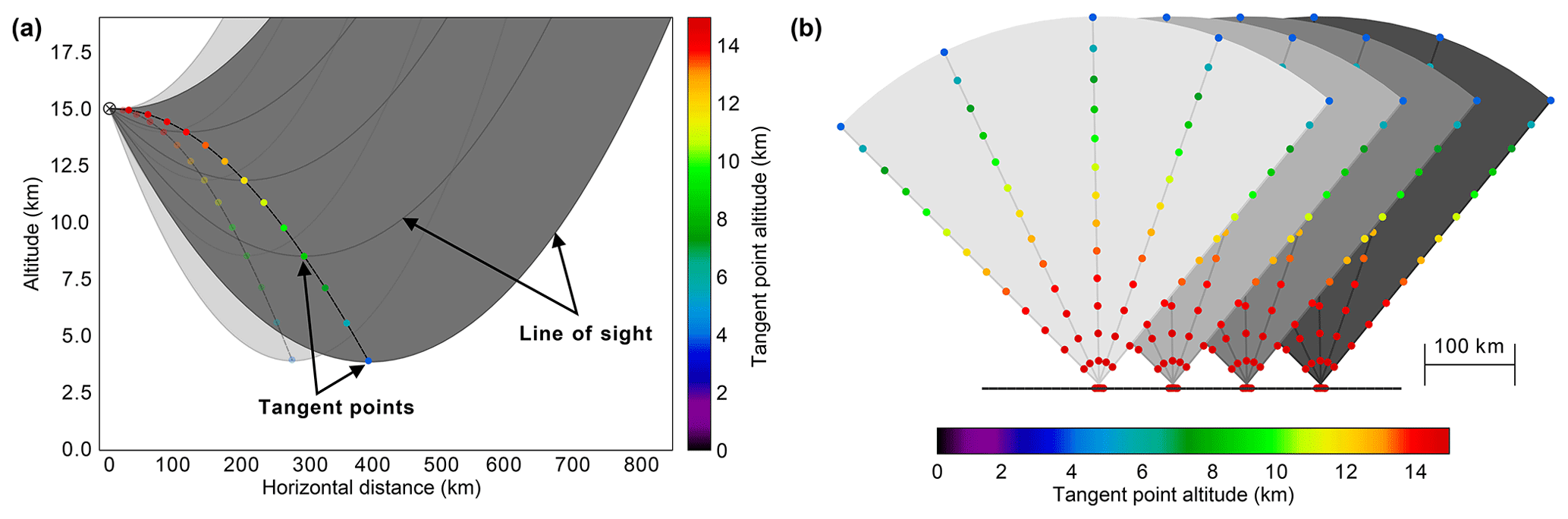
Figure 1Vertical (a) and horizontal (b) cross sections of the limb-sounding geometry of airborne GLORIA measurements using the LAT configuration. The tangent points of GLORIA measurements are shown as coloured dots, where the colour indicates the tangent point altitude. In panel (a), the flight direction points into the plane of the paper. The line of sight (LOS) of GLORIA, which is a straight line in reality, has a parabolic shape in this plot due to the transformation into a Cartesian coordinate system with the x axis following the Earth surface. The dark grey lines depict exemplary the LOSs of five distinct rows of the GLORIA detector for images taken under 90∘ azimuth angle. The LOSs of all other detector rows lie within the dark-grey shaded area. The respective tangent points are shown in bright colours. The configuration for forward- and rearward looking images is shown in light grey (LOSs) and pale colours (tangent points). The tangent points of forward- and rearward-looking images are closer to the flight path than those of images taken under 90∘ azimuth angle. (b) Top–down view of the flight path of LAT. The dots again indicate the tangent points and are coloured according to their altitude. Each grey sector indicates one horizontal scan from 45 to 135∘. The lighter the grey, the later in time the measurements are taken. Figure taken from Krisch et al. (2018).
2.2 Temperature retrieval for the Atmospheric Infrared Sounder (AIRS)
The Atmospheric Infrared Sounder (Aumann et al., 2003; Chahine et al., 2006; AIRS) is a nadir-scanning instrument onboard NASA's Earth Observing System (EOS) Aqua satellite that performs scans across the satellite track. Each scan consists of 90 footprints across track, and the width of the swath is about 1800 km. At nadir, the footprint diameter is 13.5 km, and the across-track sampling step is 13 km. The along-track sampling distance is 18 km. The EOS Aqua satellite is in a sun-synchronous orbit with fixed Equator crossing times of 13:30 LT for the ascending orbit (flying northward) and 01:30 LT for the descending orbit (flying southward).
AIRS is a hyperspectral sounder that measures atmospheric emissions of CO2 and other trace gases with high spectral resolution. In contrast to the limb geometry, nadir sounding depends on the optical depth along the line of sight to gain vertical information. Depending on the wavelength, the sensitivity function along the line of sight peaks at different altitudes (Hoffmann and Alexander, 2009). By combining multiple spectral channels, a temperature altitude profile can be retrieved. In contrast to limb sounders, the vertical resolutions of these nadir profiles are usually on the order of 10 km in the stratosphere.
For retrievals of night-time data, emissions in the 4.3 µm and the 15 µm spectral bands can be combined. For daytime retrievals only the 15 µm band is used due to non-local thermodynamic equilibrium effects which influence the 4.3 µm band. Correspondingly, AIRS night-time data have a better vertical resolution and lower noise. Except at polar latitudes, daytime data correspond to ascending orbits and night-time data to descending orbits. The AIRS temperature retrievals presented in this paper follow the retrieval set-up presented by Hoffmann and Alexander (2009). Exemplary temperature-weighting functions for midlatitude atmospheric conditions and the nadir-viewing direction are shown in Fig. 2a.
The vertical resolution of these temperature retrievals varies from 6.6 to 14.7 km depending on altitude. The total accuracy lies between 0.6 and 2.1 K, while the precision is in the 1.5–2.1 K range (Hoffmann and Alexander, 2009). The retrieval has been designed for stratospheric altitudes and provides its best results between 20 and 60 km. Validation of the AIRS temperature retrievals was conducted by Meyer and Hoffmann (2014).
In order to allow quantitative assessments of GW parameters derived from measurements, the sensitivity function of the observation technique with respect to GWs with different spatial scales has to be considered (Alexander, 1998; Preusse et al., 2000; Ern et al., 2005; Alexander et al., 2010; Trinh et al., 2016). It maps the true GW amplitude or momentum flux onto the amplitude or momentum flux observed by the given measurement technique. The AIRS sensitivity function for the retrieval used in the middle stratosphere (36 km) is shown in Fig. 2b. This sensitivity function is calculated by convolving the temperature-weighting functions in Fig. 2a with a sinusoidal 1-D temperature profile and by fitting a 1-D sinusoidal function to the resulting temperature profile. A comparison of the true (original) wavelength and amplitude with the retrieved (fitted) ones is plotted in Fig. 2b. For vertical wavelengths below 25 km, the temperature amplitude is significantly underestimated and measured vertical wavelengths in AIRS can appear up to 45 % larger than their true value. As such, AIRS measurements of vertical wavelengths below 25 km may be overestimated, so caution is advised.

Figure 2Panel (a) shows exemplary temperature-weighting functions (averaging kernels) for the AIRS retrieval of temperature at different altitudes (colour) in midlatitude atmospheric conditions and the nadir-viewing direction. In panel (b) the AIRS sensitivity function towards gravity waves with different vertical wavelengths at an altitude of 36 km is depicted. A description of how these sensitivity functions are calculated can be found in the text.
These values do not include effects caused by the scale separation of the measured temperature into background temperature and GW perturbations. Sensitivity functions including the effect of scale separation by an across-track fourth-order polynomial (a standard procedure for nadir sounders) are given, for example, by Meyer et al. (2018) or the supporting information of Ern et al. (2017). Moreover, GWs with horizontal wavelengths of less than 100 km, which may be affected by the limited AIRS footprint size, are not described by the sensitivity function in Fig. 2.
2.3 Analysis and reanalysis model data
Modern numerical weather prediction (NWP) relies on two fundamental components: first, a high-resolution global circulation model (GCM), which includes all processes relevant for weather forecasting and, second, the assimilation of a multitude of different types of measurements. The European Centre for Medium-Range Weather Forecasts (ECMWF) integrated forecast system (IFS) assimilates measurement data by the 4D-Var method (Rabier et al., 1997). The model is constrained by measurements clustered in 12 h windows from 09:00 to 21:00 UTC and from 21:00 to 09:00 UTC the next morning. However, as ECMWF tries to provide timely forecasts, measurement data arriving after 15:00 or 03:00 UTC cannot be used for the 12:00 or 00:00 UTC runs, respectively. Measurements up to an altitude of ≈40 km are used in the assimilation. ECMWF operational analysis fields are available every 6 h. These model fields provide a useful realistic background for propagation and also trigger realistic excitation of gravity waves by processes resolved by the model, i.e. mesoscale orography and spontaneous adjustment. Other gravity wave source processes such as convection are parameterised in the GCM and the emitted gravity waves are less realistic (Preusse et al., 2014). It has to be noted that the assimilation does not constrain gravity waves themselves; thus, they can develop freely from the model physics.
The dynamical core of the ECMWF GCM is based on a spectral representation of the atmosphere. The spatial resolution has been enhanced several times in the last decade. The ECMWF operational analysis for the year 2016 used in this paper uses 1279 spectral coefficients in the horizontal (corresponds to a resolution of 16 km) on 137 levels from the surface up to 80 km. Though the dynamical core could in principal resolve waves with a horizontal wavelength double the horizontal resolution, hyperdiffusion, which was introduced to provide numerical stability, limits well-resolved waves to about 10 spatial grid points (Skamarock, 2004; Preusse et al., 2014). Thus, waves of horizontal wavelengths longer than ≈150 km are fully resolved in the ECMWF operational analysis fields. Shorter waves, if excited, e.g., by topography, may still be present but are suppressed in amplitude.
Besides the above-described ECMWF operational analysis fields, this paper also makes use of ECMWF Reanalysis 5th Generation (ERA5) data. In contrast to the ECMWF operational analysis runs, ERA5 uses all available measurement data in the 12 h assimilation windows. Additionally, ERA5 data are available every hour. However, ERA5 has a horizontal resolution of only 31 km (639 spectral coefficients), which means only gravity waves with horizontal wavelengths larger than ≈300 km are fully resolved.
In summary, the ERA5 reanalysis has a higher temporal but lower horizontal resolution than the ECMWF operational analysis. Hence, for small-scale waves the ECMWF operational analysis is more accurate, but for fast-changing situations, ERA5 might be preferable.
2.4 Scale separation of atmospheric variables
The atmospheric temperature structure in the mid-latitude stratosphere and troposphere is shaped by dynamical features of different spatial and temporal scales. The most important features are the mean atmospheric temperature, global and synoptic-scale planetary waves, and small-scale processes including GWs. The mean atmospheric temperature is governed by slow radiative processes and large-scale meridional circulations. These vary slowly in altitude and latitude but are assumed to remain constant in a zonal direction. Planetary waves surround the Earth on latitude circles. Thus, they have integer zonal wave numbers. In the mid-stratosphere, the main planetary wave modes have zonal wave numbers of 1–6. In the lower stratosphere and troposphere, planetary waves with higher zonal wave numbers also exist. GWs have horizontal wavelength scales of a few kilometres to several thousand kilometres. However, due to the resolution of GLORIA measurements and the spatial extent of the measurement volume, we will focus here on the identification of mesoscale GWs with horizontal wavelengths between ≈100 and ≈1000 km.
For global data sets, background and GW fluctuations are often separated using zonal filtering with a cut-off wave number of 6 in the mid-stratosphere (e.g. Fetzer and Gille, 1994; Ern et al., 2006, 2018). As the region of interest in this paper is given by the GLORIA measurement altitude, which is in the lower stratosphere and upper troposphere, zonal filtering with a higher cut-off wave number 18 is required (Strube et al., 2020) and used for all global data sets (ECMWF and ERA5). As this zonal filter might still allocate GW structures with long zonal but short vertical and/or meridional wavelengths to the background, a sliding polynomial smoothing with a Savitzky–Golay filter (SG filter; Savitzky and Golay, 1964) in the vertical and meridional direction is applied additionally to the background field to suppress these small-scale signals: for the analysis and reanalysis model data used in this paper, a fourth-order SG filter over a window of 5 km in the vertical direction and a third-order SG filter over a window of 750 km in the meridional direction are used. By subtracting the smooth background temperature from the total temperature, one receives a perturbation field containing different small-scale processes like GWs or different weather systems like convection or fronts.
Due to the local nature of GLORIA measurements, global filtering algorithms, like the zonal method described above, are not suitable. Different local filtering methods for GLORIA-like data sets were tested (Appendix A) and best results were achieved with three sequentially applied third-order SG filters with windows of 750 km in each horizontal and 3 km in the vertical direction.
2.5 Spectral analysis using a three-dimensional sinusoidal fitting routine (S3D)
To characterise the temperature perturbations obtained from the scale separation described in the previous section with regard to GWs, wave parameters (horizontal and vertical wavelengths, wave amplitude, and wave direction) are derived. For this task, a small-wave decomposition method called S3D was used (Lehmann et al., 2012). S3D uses a least square approach to fit a sine function to the 3-D temperature perturbation field T′(x):
with weighting function and the sine function
with 3-D wave vector , temperature amplitude , wave phase ϕ, sine amplitude , and cosine amplitude . To reduce the impact of measurement data with low confidence values, a weighting function is used for the GLORIA data, which is chosen to be 1 if a tangent point exists in the corresponding grid cell of the retrieval and 105 if not.
The method is applied on analysis cubes – small three-dimensional subregions of the perturbation field. In each cube, a superposition of monochromatic sine waves is assumed and determined by fitting. The quality of the fits depends on the cube size. If the cubes are too large compared to the resulting wavelengths, small fluctuations get masked by larger-scale waves. Additionally, the cube should not be too large since real GWs are highly variable and complex, and an approximation with monochromatic waves is only valid inside small areas (Appendix of Krisch et al., 2017). However, if the cubes are too small, the number of data points is insufficient to uniquely identify the dominant wave structure. Systematic tests with synthetic waves have shown that cubes covering only 40 % of one wave cycle per direction still lead to reasonable results for the wave vector k.
The temperature perturbations derived from GLORIA measurements are highly variable in amplitude. To recover these variations and still keep the cube sizes large enough for reasonable fits of the wave vector k, a stepwise fitting routine is used. First, the wave vector is fitted in large cube sizes and, second, the wave amplitude and phase ϕ are determined in smaller cube sizes using the wave vectors from the larger cubes.
2.6 Ray tracing of gravity waves
The Gravity wave Regional Or Global RAy Tracer (Marks and Eckermann, 1995; Eckermann and Marks, 1997, GROGRAT) is used to study the propagation of the observed GWs. GROGRAT was the first GW ray tracer to implement the full dispersion relation
This equation relates the temporal wave properties (intrinsic wave frequency ω) with the spatial wave properties (wave vector ) and the atmospheric background properties (buoyancy frequency N, Coriolis frequency f, and density scale height H). Only this full dispersion relation enables the propagation of GWs of all frequencies, including non-hydrostatic GWs as well as GWs with frequencies close to the Coriolis frequency f, through a spatially slowly varying background atmosphere (Marks and Eckermann, 1995). In a second version of GROGRAT (Eckermann and Marks, 1997), a not only spatially but also temporally varying background atmosphere has been implemented.
The differential equations and , , are solved for multiple time steps using Runge–Kutta methods. For each time step, the wave action conservation law and the full dispersion relation are applied to calculated changes in the wave amplitude. Changes in the ground-based frequency due to temporal variation in the background field are implicitly taken into account by this method. Wave dissipation and damping () are accounted for in GROGRAT by including turbulent (Pitteway and Hines, 1963) and radiative (Zhu, 1994) damping schemes and saturation (Fritts and Rastogi, 1985).
The spatially and temporally varying background atmosphere has been constructed from 6-hourly ECMWF operational analysis fields as described in Sect. 2.4. In addition, GROGRAT applies a third-order spline interpolation in both space and time. The start parameters necessary to launch GWs into these background fields are obtained by the sinusoidal fits described in Sect. 2.5.
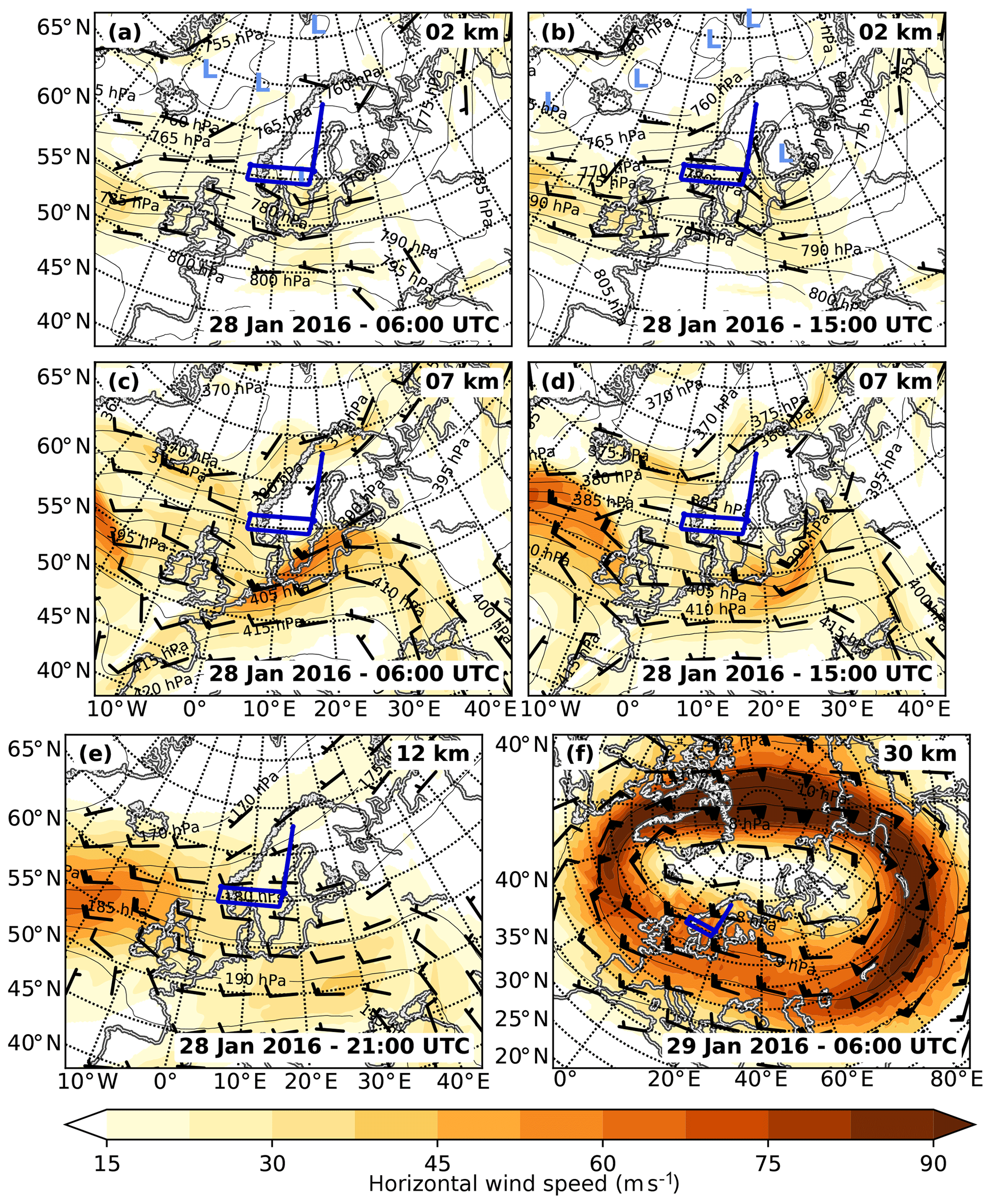
Figure 3Synoptic situation over northern Europe on 28–29 January 2016. Shown are ERA5 horizontal wind (colour and barbs) and pressure (contour lines) fields at different altitudes and time steps. Low-pressure systems are marked with a light blue “L”. The altitude of the respective cross section is always given at the top right of the panel and the model time at the bottom right. The dark blue line marks the flight path.
3.1 Aircraft campaign
From December 2015 to March 2016 an extensive aircraft measurement campaign took place with ground bases in Oberpfaffenhofen, Germany, and Kiruna, Sweden. This campaign was a conglomerate of several campaigns with different scientific goals, among them to study the full life cycle of GWs (GW-LCYCLE) and to demonstrate the use of infrared limb imaging for GW wave studies (GWEX). The carrier used for this campaign was the German High Altitude and Long Range Research Aircraft (HALO; DLR, 2018). This plane is based on the business jet Gulfstream G550 with modifications that allow mounting a wide variety of scientific equipment.
The scientific payload of HALO during the winter 2015/2016 campaign encompassed three remote-sensing instruments: GLORIA in the belly pod, an upward-looking water vapour, cloud, and ozone lidar (WALES), and a differential optical absorption spectrometer (DOAS). In addition, the Basic HALO Measurement and Sensor System (BAHAMAS; Giez, 2012) measuring temperature, pressure, and winds at high precision and high temporal resolution as well as a number of in situ instruments measuring trace gases were part of the payload. A more detailed overview of all instruments is given in Oelhaf et al. (2019).
During the campaign, 18 scientific research flights adding up to 156 flight hours were performed covering 20 to 90∘ N and 80∘ W to 30∘ E. Seven of these scientific research flights contained measurements of GWs. This paper presents and analyses GLORIA measurement results from a gravity wave flight on 28 January 2016 above southern Scandinavia.
3.2 Synoptic situation
For 28 January 2016, the ECMWF-IFS predicted gravity waves above southern Scandinavia. One prominent source of gravity waves in this region are the Scandinavian Mountains also known as Scandes. The Scandes is a mountain ridge running north–south along the west coast of Scandinavia. In the southern part close to the flight track, the mean width of the ridge is around 250 km and the mean elevation is on the order of 1300 m. According to linear wave theory (e.g. Nappo, 2012), the intrinsic frequency of a mountain wave ω can be calculated from the horizontal terrain wave number kh and the horizontal background wind U0 perpendicular to the ridge extent:
Due to the ridge's width l, the maximum horizontal wavelength λh of gravity waves generated by this orography should be on the order of 400–500 km (). As the intrinsic frequency range of GWs is restricted to , the wind at the surface to generate mountain waves with a horizontal wavelength of 400 km at a latitude of 60∘ N has to be at least . However, waves generated with such slow wind speeds would have very low vertical group velocities and small saturation amplitudes. Both in the forecast of ECMWF-IFS (not shown) and ERA5 reanalysis (Fig. 3a) the flow over the southern part of the Scandes is around 17.5 m s−1 in the morning of 28 January 2016. According to theory, a gravity wave with a horizontal wavelength of 400 km, which is generated by a flow over orography with such a wind speed, has a vertical group velocity of 0.86 km h−1 and needs 14 h to propagate to an altitude of 12 km (GLORIA measurement altitude). Thus, the flight time between 17:30 and 22:00 UTC fits in very well with this situation. As the orography of the Scandes is composed of mountain ridges with many different heights and widths, a complex wave structure with many different horizontal wavelengths is expected.
Furthermore, a low-pressure system evolved over southern Scandinavia in the morning of the measurement day, which then moved slowly eastward (Fig. 3a and b). This low-pressure system forced the eastward jet stream in the upper troposphere to slow down and diverge. Thus, a jet-exit region was created over the North Sea between Scandinavia and Great Britain (Fig. 3c). This jet-exit region was following the low-pressure system slowly eastwards. Both jet-exit regions as well as convective storms, which often accompany low-pressure systems, are prominent sources of gravity waves and were located in the vicinity of southern Scandinavia on this day (Fig. 3d). Hence, the observed gravity waves could be expected to be a mixture of waves generated by orography, the jet-exit region, and convection.
The divergence in the jet stream was also connected with a low tropopause altitude and accordingly a low cloud top height of around 8 km above southern Scandinavia, which results in good measuring conditions for GLORIA. However, it also sharpened the tropopause, which can lead to a partial reflection of gravity waves. The horizontal wind kept its eastward orientation at higher altitudes (Fig. 3e and f) as the maximum of the circumpolar jet stream on this side of the pole was located just south of Scandinavia. This provided favourable conditions for vertical GW propagation.
3.3 GLORIA measurements and diagnostics
The GW structure was probed with multiple, 700 km long, linear flight legs crossing southern Scandinavia in zonal direction (see Fig. 4). To study the interaction of the GWs with the tropopause by in situ observations (Gisinger et al., 2020), two flight legs were positioned below (legs 1 and 2) and two flight legs above the tropopause (legs 3 and 4). Both lower legs were performed at 61∘ N (leg 1 from point A to point B and leg 2 from point B to point A) and were mainly dedicated to in situ and water vapour observations by BAHAMAS and WALES. GLORIA did not measure during these low-level legs, as this part of the flight was mainly inside or just above clouds. At 20:00 UTC, HALO ascended to almost 13 km and performed an east–west leg at 59.5∘ N (leg 3 from point C to point D). This flight leg was placed further to the south, so GLORIA could look at the lower flight legs perform earlier (between A and B), which should allow comparisons with in situ and lidar data. Unfortunately, the cloud cover prohibited GLORIA during most of the flight leg to collect measurements down to the former flight altitude. At the westernmost point of the leg (point D), HALO went northward back to the original latitude of 61∘ N (point B) and ascended further to ≈13.5 km altitude. A last west–east leg (leg 4 from point B to point A) was performed before returning to the campaign base at Kiruna.
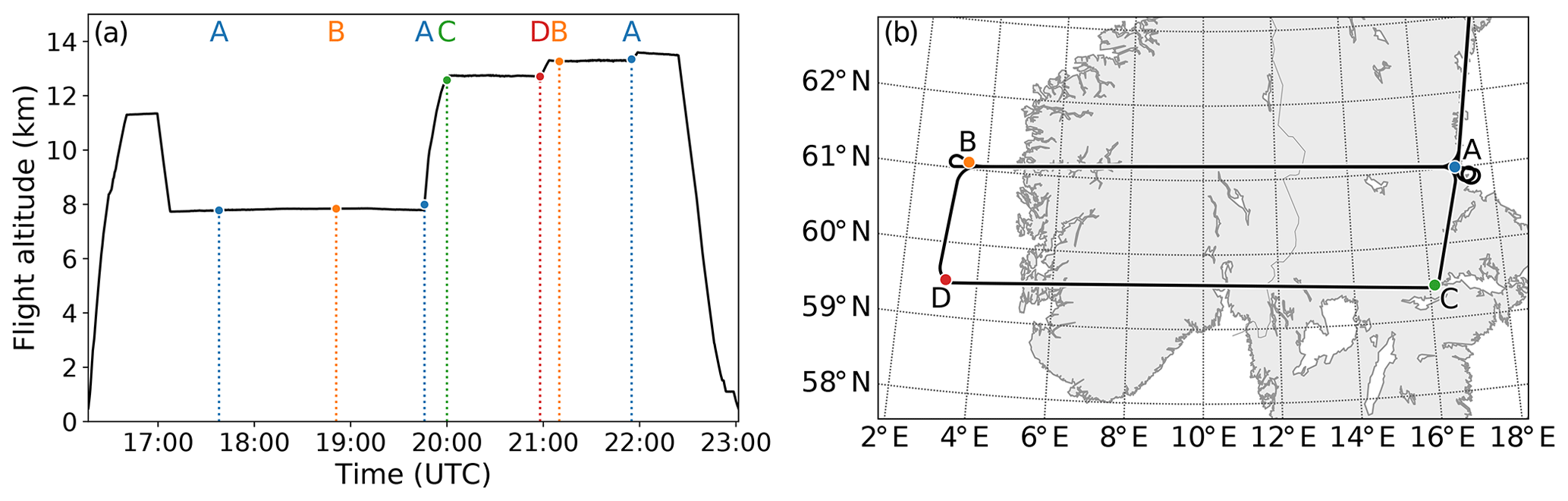
Figure 4HALO flight over southern Scandinavia on 28 January 2016. Panel (a) shows the different flight altitudes and (b) the geographic location. The letters and dotted lines in (a) mark the point in time at which the respective geographic locations in (b) are reached.
Because jet-generated GWs are not necessarily stationary, linear-flight tomography (LAT) was chosen as GLORIA's measurement strategy, and two separate retrievals were performed using measurements taken during flight leg 3 (southern leg) and flight leg 4 (northern leg). Both retrievals have a horizontal resolution of 30 km in flight direction and 70 km perpendicular to flight direction. The vertical resolution is 400 m, the precision is better than 0.05 K, and the accuracy, including misrepresented background gases, uncertainties in spectral line characterisation, uncertainties in instrument attitude, and calibration errors, is better than 0.7 K. A detailed description of how these retrieval diagnostics are calculated can be found in Krisch et al. (2018).

Figure 5A comparison of the GLORIA retrieval results with in situ temperature measurements and ECMWF operational analyses. The GLORIA retrievals and ECMWF model data were interpolated in space onto the flight path. The shaded area indicates the time period from which GLORIA measurements were included in the respective retrieval: the southern leg retrieval only uses measurements taken between 20:00 and 20:55 UTC, and the northern leg retrieval only those taken between 21:05 and 21:55 UTC. Values in the non-shaded area are extrapolated in space to the flight path performed earlier or later. The black curve shows the flight altitude.
The GLORIA southern leg retrieval results agree well with the in situ temperature measurements of BAHAMAS taken on the southern flight leg (Fig. 5a between points C and D). The same is valid for the northern leg retrieval results and BAHAMAS measurements from the northern leg (Fig. 5b between points B and A). Some very small scales are beyond the spatial resolution of GLORIA. In situ measurements taken during the northern (southern) flight leg, show stronger deviations when compared to extrapolated GLORIA data from the southern (northern) leg retrieval. However, the main wave structures are still captured. This can be explained by the temporal difference between the two legs and the location of the tangent points of the respective retrievals: the tangent point altitude decreases with distance to the flight path (see Fig. 1). Hence, the tangent points of measurements taken on the southern flight leg are roughly 2.5 km below the flight altitude of 13.5 km of the northern flight leg at 61∘ N and vice versa. A comparison of in situ measurements taken, for example, on the northern flight leg with the temperature retrieval using measurements from the southern flight leg thus not only differs in measurement time but also relies on vertical and/or horizontal data extrapolation. The agreement is still much better than with the a priori temperature.
The large differences between the ECMWF operational analyses on 28 January 2016 at 18:00 UTC and 29 January 2016 at 00:00 UTC illustrate the high temporal variability of the gravity wave structure. The ECMWF operational analysis at 18:00 UTC in general agrees very well with the GLORIA and BAHAMAS measurements: it catches the main variations, but the temperature oscillations associated with the GWs are not as detailed as observed by the different measurement techniques. Sometimes the wave structure appears to be shifted in time or space compared to GLORIA and in situ measurements (e.g. between 20:30 and 20:45 UTC).
This comparison with both in situ measurements and ECMWF operational analysis demonstrates the high quality of the tomographic reconstruction of the temperature field from GLORIA measurements and proves LAT using GLORIA capable of reconstructing highly complex gravity wave structures.
4.1 Wave characterisation
The temperature retrievals are separated into background atmosphere and GW perturbations using a third-order Savitzky–Golay filter with window lengths of 750 km in both horizontal and 5 km in the vertical direction (see Sect. 2.4 and Appendix A for details). For this filtering, the retrieval data are expanded in all spatial directions with a priori data to avoid edge effects. The remaining temperature perturbations can be seen in Fig. 6. Figure 6a, c, and e show the temperature perturbations derived from the retrieval using measurements taken during the southern flight leg, and Fig. 6b, d, and f show those derived from the retrieval using measurements taken during the northern flight leg.
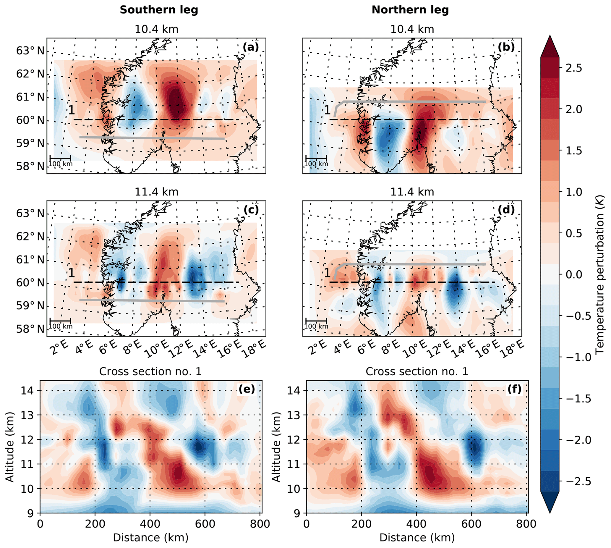
Figure 6Temperature perturbations of the GLORIA tomographic retrieval for the flight on 28 January 2016 over southern Scandinavia. Shown are horizontal (a–d) and vertical (e and f) cross sections. The vertical cross sections are along the dashed lines in (a)–(d). The grey line indicates the flight path. Panels (a), (c), and (e) show results from measurements taken on the southern flight leg; panels (b), (d), and (f) show results from measurements taken on the northern flight leg.
The GLORIA retrievals for both flight legs show a prominent wave structure with ≈400 km horizontal and ≈6–7 km vertical wavelength. This large-scale gravity wave (LSGW) is perturbed by a smaller-scale gravity wave (SSGW) with a longer vertical but shorter horizontal wavelength. This SSGW is more prominent in the east at lower altitudes (10.4 km; Fig. 6a and b) and in the western part at higher altitudes (11.4 km; Fig. 6c and d). The LSGW has the strongest amplitudes of about 3 K between 10 and 14∘ E.
Even though the main characteristics are similar for the observations during both legs, there are some differences between them. The LSGW appears to have a slightly different horizontal orientation in the two different retrievals: in the southern leg retrieval between 60 and 62∘ N the phase fronts are oriented north–south (Fig. 6a and c), whereas the phase fronts in the northern leg retrieval seem to be turned slightly and have a north–north-east to south–south-west alignment between 59 and 60.5∘ N. Also, the horizontal wavelengths of the LSGW and the steepness of the phase fronts seem to differ slightly between the two retrievals. These differences can either originate from the slight difference in the location of the measurements used for the two retrievals or the difference in time.
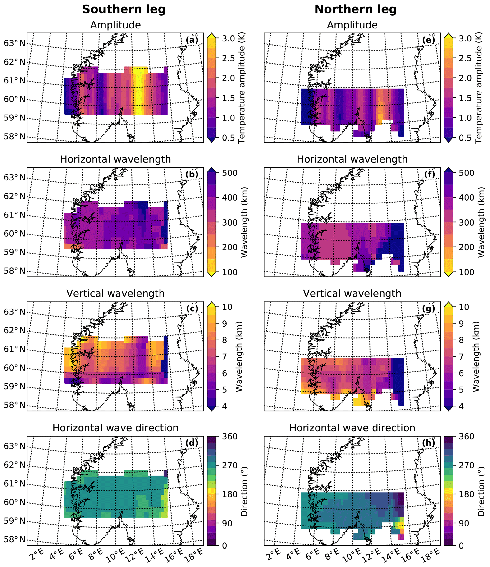
Figure 7Three-dimensional sinusoidal wave fit of the GLORIA measurements at a centre height of 11.4 km in fitting cubes of km3 with a tangent point weighting according to Sect. 2.5. In order to capture the spatial variation in the amplitudes, an amplitude and phase refit has been performed in fitting cubes of km. Panels (d) and (h) show the direction of the horizontal wave vector. The eastward direction corresponds to 90∘ and the southward direction to 180∘.
The temperature perturbation fields from both retrievals were spectrally analysed with a 3-D sinusoidal fitting routine in overlapping fitting cubes of 400 km zonal, 250 km meridional, and 4 km altitude extent (see Sect. 2.5 for details). Horizontally, this cube size is of the same order of magnitude as the wavelength. Vertically, the cube roughly encompasses the whole measurement space. To capture the spatial variation in the wave amplitude, refits of amplitude, and wave phase, using the previously determined wave vector k, have been performed in smaller sub-cubes of 100 km zonal, 250 km meridional, and 1 km altitude extent.
With these settings, the spectral analysis is only capable of identifying the LSGW component. The results (Fig. 7) confirm the change in horizontal direction of the LSGW between both retrievals already observed in Fig. 6: the wave orientation changes from in the southern flight leg retrieval to in the northern flight leg retrieval (Fig. 7d and h). Furthermore, the horizontal wavelength increases slightly in both retrievals from west to east (Fig. 7b and f). In the southern leg retrieval, the waves decrease in steepness (decreasing vertical wavelength) from west to east (Fig. 7c), which can also be seen in the vertical cross section of the temperature perturbations (Fig. 6e): at 200 km distance along the cross section, the waves have shorter horizontal and longer vertical wavelengths than at 600 km. According to the sinusoidal fit, the LSGW has the highest amplitudes between 12 and 14∘ E (Fig. 7a and e). The LSGW in the northern flight leg retrieval is, in general, steeper than those of the southern flight leg retrieval (Fig. 7c vs. g), a property already visible in the temperature perturbations (Fig. 6).
After the LSGW has been identified in both retrievals, it can be subtracted from the temperature perturbation fields to reveal more clearly the SSGW. The remaining SSGW fields are shown in Fig. 8. Here, SSGWs with amplitudes of up to 1.5 K with short horizontal (around 100 km) and very long vertical wavelengths (up to infinity) can be seen. However, the SSGW structure is quite complex and no single monochromatic wave can be identified by eye. Instead, the structure has very localised maxima and similarity to a chequerboard. This is an indication for the simultaneous presence of at least two wave packets with different propagation directions and might be caused by the presence of either upward- and downward- or eastward- and westward-propagating waves. There is no indication of a symmetric source, which could explain eastward- and westward-propagating wave packets. Additionally, any intrinsically eastward-propagating waves would have very high ground-based phase speeds and periods and, hence, would not be observable by GLORIA. Simultaneous upward and downward wave propagation might hint at a reflection layer somewhere above the measurement altitude.
It is not only the LSGW component that changes in time: the phases of the SSGW component shift further to the east around an altitude of 11.4 km from southern to northern leg retrieval (Fig. 8). This can be seen, for example at the maximum at 8∘ E, which is located slightly to the left of the meridian for the southern retrieval, whereas it is on the meridian for the northern retrieval. The two maxima between 10 and 11∘ E show a similar behaviour. These differences help to explain why a joint retrieval using measurements of both legs simultaneously did not converge properly.
As the sinusoidal fitting routine is currently only tested for fits of one monochromatic wave at a time, chequerboard patterns cannot be resolved. To spectrally analyse the observed SSGW field with the method described in Sect. 2.5, the fitting routine would have to be further tested and potentially adjusted. These results provide guidelines for the future development of the S3D method.
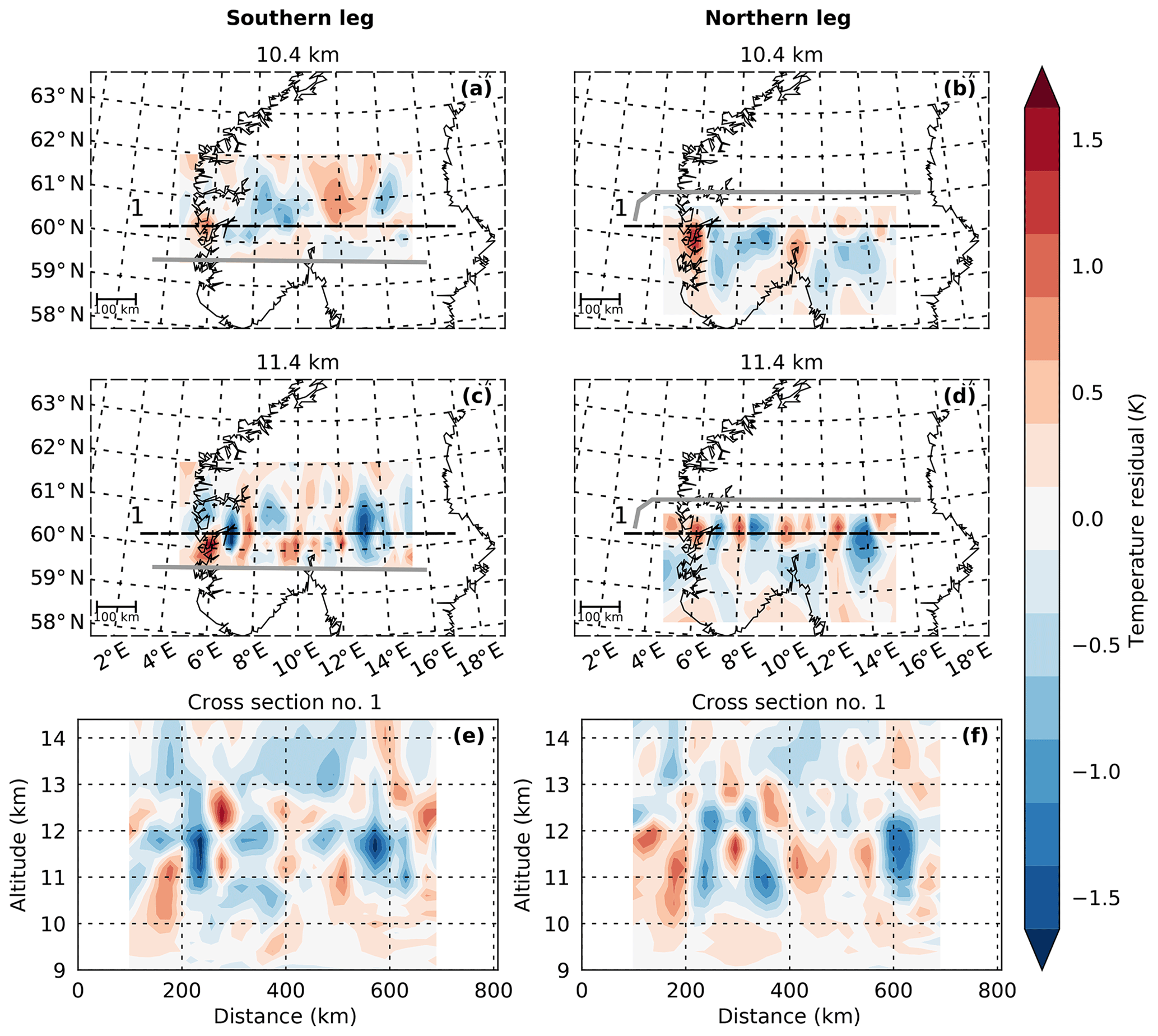
Figure 8Remaining temperature perturbations of the GLORIA tomographic retrieval after the subtraction of the wave of Fig. 7. Shown are horizontal (a–d) and vertical (e and f) cross sections. The vertical cross sections are along the dashed lines in (a)–(d). The grey line indicates the flight path.
4.2 Wave sources and propagation
In order to identify the sources of the LSGW component, ray-tracing calculations with GROGRAT have been performed (Sect. 2.6). Such ray-tracing calculations need very accurate GW starting parameters (see Appendix of Krisch et al., 2017), which could be obtained by the sinusoidal fit only for the LSGW component. Thus, only the sources of the LSGW are analysed in the following.
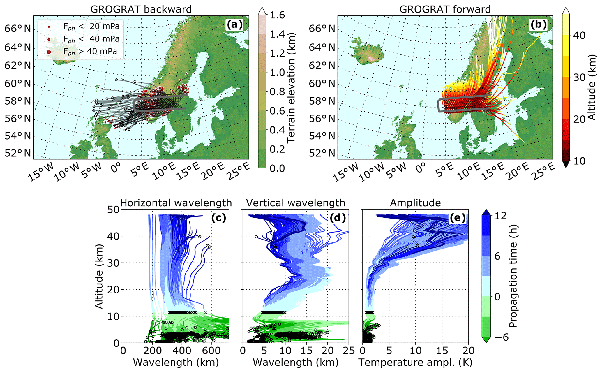
Figure 9GW ray traces calculated using the GROGRAT model. Panel (a) shows the backward ray traces and panel (b) the forward ray traces. Panels (c)–(e) show the change in wave parameters with height. The end points of backward rays which do not reach the surface are marked with an open circle; rays which reach the surface are indicated with a red dot. The size of the circle marks the strength of the wave (GWMF). In panels (c)–(e), the crosses indicate the wave properties at flight altitude for waves that do not reach the surface. However, no obvious pattern can be observed.
Most of the backward rays of the LSGW component and especially those with the highest gravity wave momentum flux (GWMF) values are traced back to the Scandes (Fig. 9a). However, other rays and especially those not reaching the surface originate from a widespread area west of Scandinavia. According to ERA5 (Sect. 3.2), a jet-exit region as well as a low-pressure system were moving over this area during the course of 28 January 2016. Both might be the source of these non-orographic GWs. At the measurement altitude, the wave parameters of waves not originating from the surface (Fig. 9c–e, black crosses) do not differ significantly from those generated by orography.
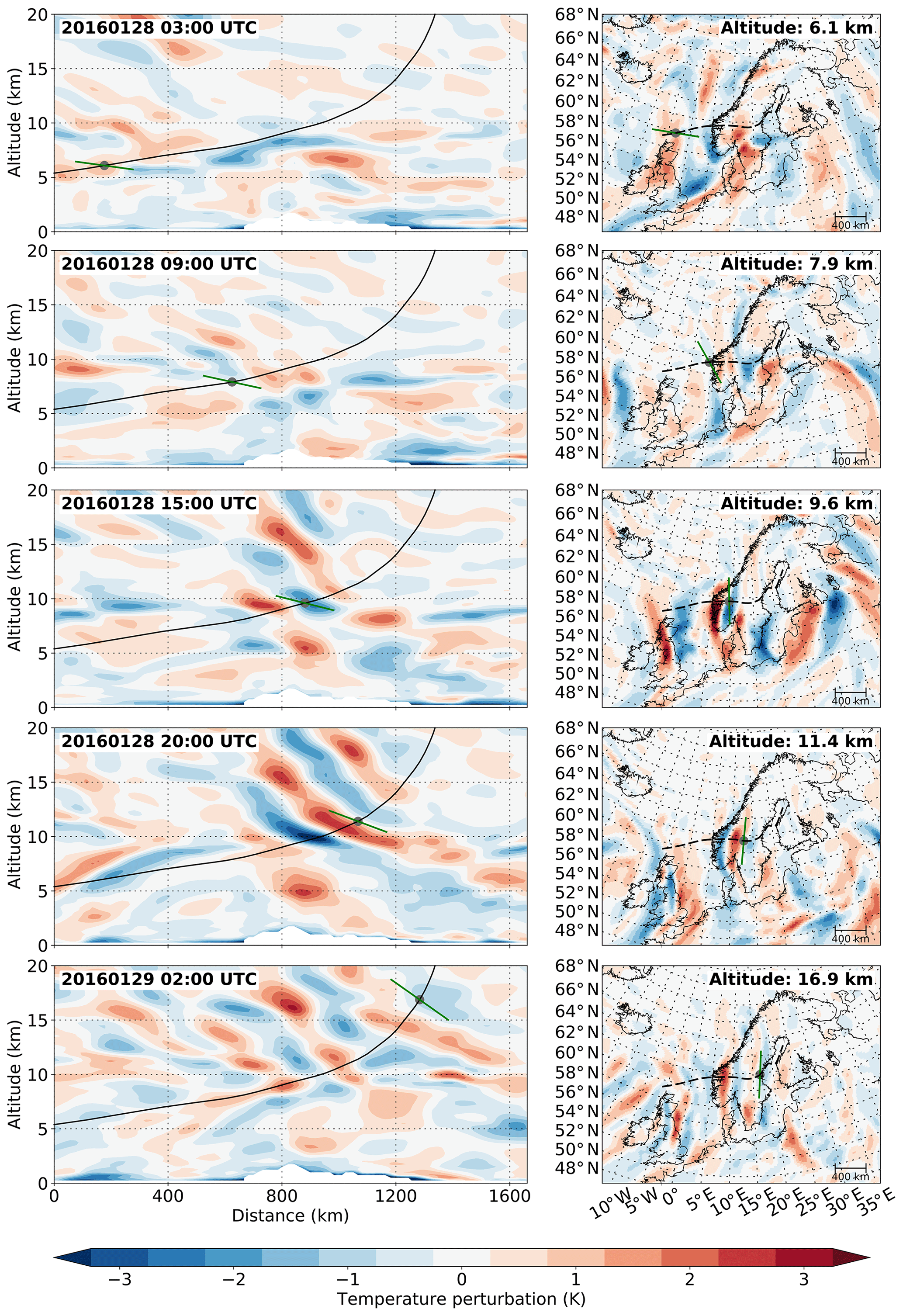
Figure 10Cross sections through different ERA5 temperature perturbations along an example GROGRAT ray trace originating from GLORIA measurements. The left column shows vertical cross sections along the ray trace (black line). The grey dot marks the location of the ray trace at the respective time step of the model. The green line shows the orientation of the phase lines as predicted by GROGRAT. The right column shows horizontal cross sections at the altitude of the ray path at the respective model time.
The sources of these waves are further examined by comparing the ray-tracing results with ERA5 (Fig. 10). One ray trace has been chosen as a non-orographic GW reference case, and ERA5 cross sections are plotted along its path. The wave source can be located at any point along the backward trajectory of the ray tracer. In the early morning at 03:00 UTC, the GW predicted by the ray tracer does not agree well with ERA5. Thus, the source of the wave might be further towards the measurement location. At 09:00 UTC a wave structure with a similar orientation to the one predicted by the ray tracer can be found just in front of the Scandinavian coast in ERA5. However, the orientation of the wave is not aligned with the main mountain ridge. Moreover, the location of the wave is still off the coast and not above the mountain range. Both elements suggest an excitation by a non-orographic source.
At 15:00 UTC, a wave field located directly above the mountains and reaching up to 20 km appears in ERA5. However, the wave structure at 10 km altitude, i.e. the exact location of the traced wave, differs in steepness from the fields above and below. At 20:00 UTC, the time of the measurement flight, this slightly flatter structure has propagated a bit further. In the horizontal cross section, the cold front (blue) has an orientation more or less parallel to the main mountain ridge south of 62∘ N. North of 62∘ N, the orientation changes and agrees well with the prediction of the ray tracer. At 02:00 UTC on the following day, one can now clearly identify different wave packets both in the horizontal as well as in the vertical cross section. The wave packet followed by the ray tracer is less steep than the waves above the mountains and is now located further to the east. This comparison suggests that a non-orographic wave packet has travelled through an orographically excited wave above the Scandes during the course of the late afternoon and night of the measurement day. This again explains why the retrieval of both flight legs simultaneously did not converge: the temperature perturbations caused by the non-orographic wave were not sufficiently stationary.
Forward ray tracing shows that the waves propagate slightly northward and to high altitudes (Fig. 9b). The temperature amplitude increases with height and reaches values between 10 and 30 K just below 40 km. The waves take between 3 and 12 h to propagate to these altitudes. The exact propagation time strongly depends on the wavelength: gravity waves with long vertical and short horizontal wavelengths (steep waves) rise faster than those with shorter vertical and longer horizontal wavelengths. The horizontal wavelengths stay on the order of 200–400 km. The vertical wavelengths double from 5–10 km at GLORIA measurement altitude to around 10–20 km at an altitude of 20 km and stay more or less constant above. This doubling of the vertical wavelengths is the result of a Doppler shifting caused by a doubling of the horizontal wind from 30 m s−1 at 12 km to 60 m s−1 above 20 km altitude (Fig. 3).
4.3 Comparison to AIRS measurements
To investigate the accuracy of the forward ray-tracing calculations of the GROGRAT model, the propagation results are compared to AIRS satellite measurements. GROGRAT predicts the GWs to take between 3 and 12 h to propagate from GLORIA measurement altitudes up to 36 km. Thus, AIRS measurements of the descending orbit on 29 January 2016 were chosen for the comparison (Fig. 11). These measurements over Scandinavia were taken between 01:00 and 03:00 UTC that is between 3 and 6 h after the HALO flight took place. The forward ray tracing predicts GW amplitudes between 10 and 30 K above middle and northern Scandinavia (Fig. 9e). The vertical wavelengths are predicted to be roughly between 7 and 17 km (Fig. 9d). According to the AIRS sensitivity function (Fig. 2b) such GWs are underestimated in amplitude by roughly 80 % and overestimated in vertical wavelength by around 20 %. Thus, these waves should appear only weakly in the AIRS measurements and with wavelengths of around 18 km. This is confirmed by the AIRS temperature perturbations at 27 and 36 km (Fig. 11): above 60∘ N only faint wave-like perturbations are visible. Sinusoidal fits of the AIRS data in cubes reaching from 26 to 46 km show enhanced amplitudes above the southern tip of Scandinavia and the North Sea (Fig. 12a), where the mid-stratosphere wind velocities are higher (cf. Fig. 3f). Above middle and northern Scandinavia, as expected, very low amplitudes are identified with vertical wavelengths on the order of 20 km. Taking the overestimation in vertical wavelength by around 20 % into account, this matches very well with the ray-tracing results. The horizontal wavelengths derived from the AIRS measurements also comply well with the GROGRAT model results.
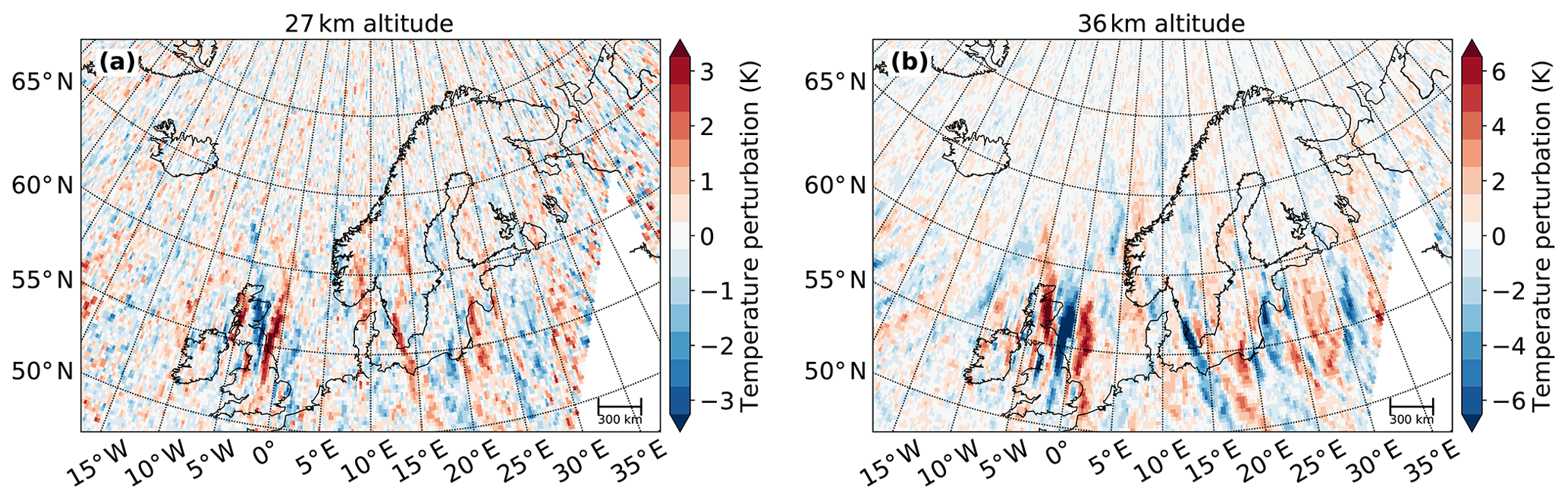
Figure 11Temperature perturbations of the AIRS retrieval at 27 km (a) and 36 km (b) for the descending orbits with Equator crossing time at 01:30 LT (between 01:00 and 03:00 UTC above Scandinavia) on 29 January 2016. Due to the exponential increase in wave amplitude with height caused by decreasing density, one might expect that a gravity wave's amplitude would increase by approximately a factor of 2 over this height range. Thus, the colour steps are chosen to be 0.5 K in panel (a) and 1 K in panel (b).
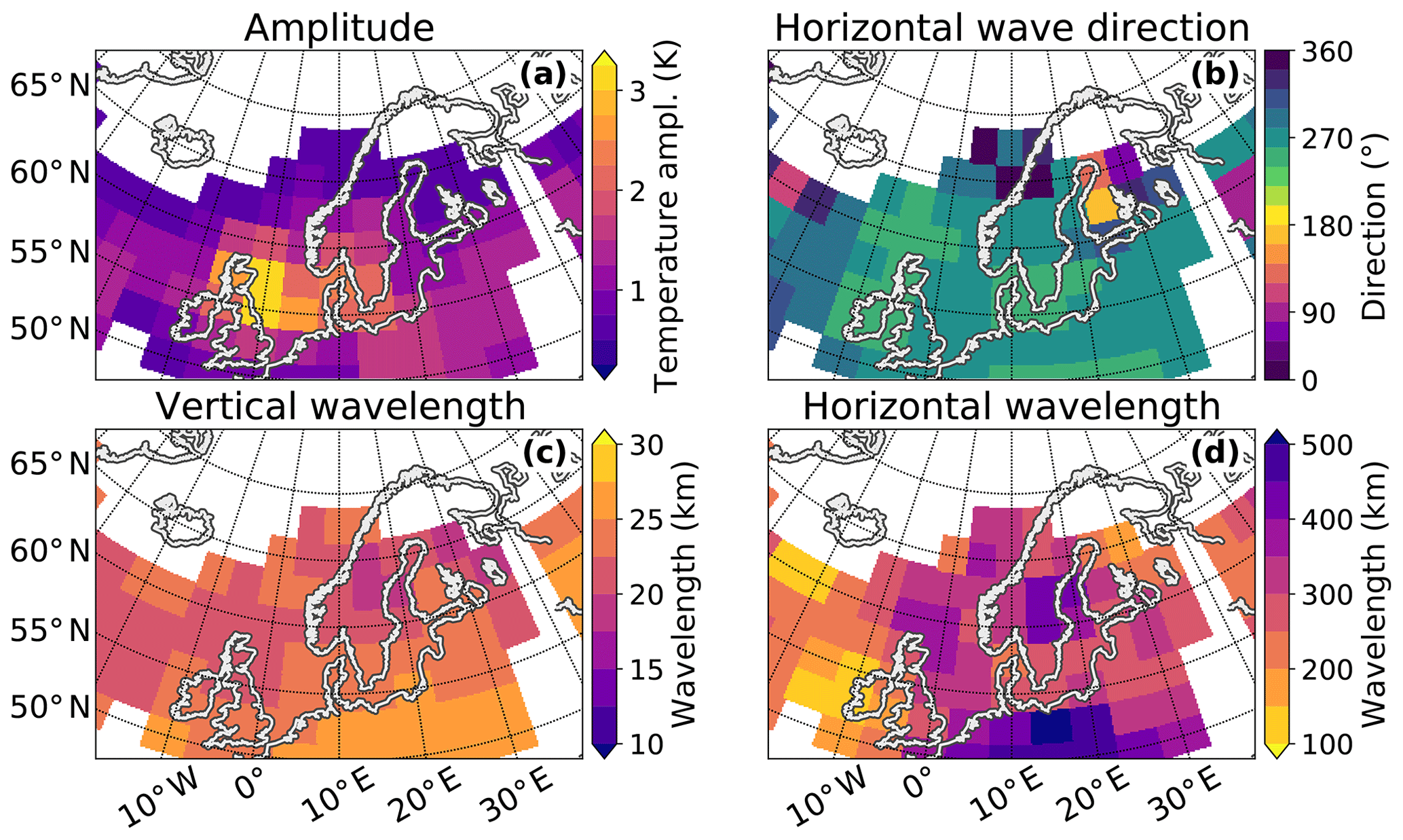
Figure 12Three-dimensional sinusoidal wave fit of the AIRS measurements based on fitting cubes of km3 at a centre height of 36 km. It has to be noted that the S3D method averages the wave amplitude over the whole cube size. This may lead to an underestimation of the amplitude in large cubes. However, due to the sparse vertical sampling of AIRS, such large cube sizes are necessary to retain reasonable fit results. Figure 11b indicates that the real amplitude is probably 1.5–2 times the S3D result in panel (a).
The influence of the AIRS sensitivity on these GWs is studied in more detail using ERA5 model data. The ERA5 temperature field is first separated into small-scale gravity wave perturbations and large-scale background motion (see Sect. 2.4). Each profile of the ERA5 GW perturbation field is then convolved with the temperature sensitivity functions of the AIRS retrieval shown in Fig. 2a, and profiles as they would be observed by AIRS are reconstructed. Cross sections of the resulting temperature perturbation field are shown in Fig. 13b, d and f. At an altitude of 27 km the original ERA5 temperature perturbation field is filled with various GWs of amplitudes on the order of 3 K (Fig. 13a). After applying the AIRS averaging kernel, only small parts of the wave structure remain visible with strongly damped amplitudes (Fig. 13b). Also the complex wave structures are replaced by mainly monochromatic wave packets. A similar picture can be seen at 36 km altitude (Fig. 13c and d). In addition to this amplitude underestimation, the vertical cross sections reveal the overestimation of the vertical wavelengths (Fig. 13e and f), which had already been predicted by the sensitivity function in Fig. 2b. In particular, the flat waves at the top right of Fig. 13e with vertical wavelengths on the order of 10 km appear with very low amplitudes and much steeper phase fronts in the AIRS simulation (Fig. 13f). A similar overestimation of vertical wavelengths by AIRS was also observed by Meyer et al. (2018) for a strong wave event over South America, when comparing AIRS measurements to those of the High Resolution Dynamics Limb Sounder (HIRDLS), which has a much better vertical resolution.
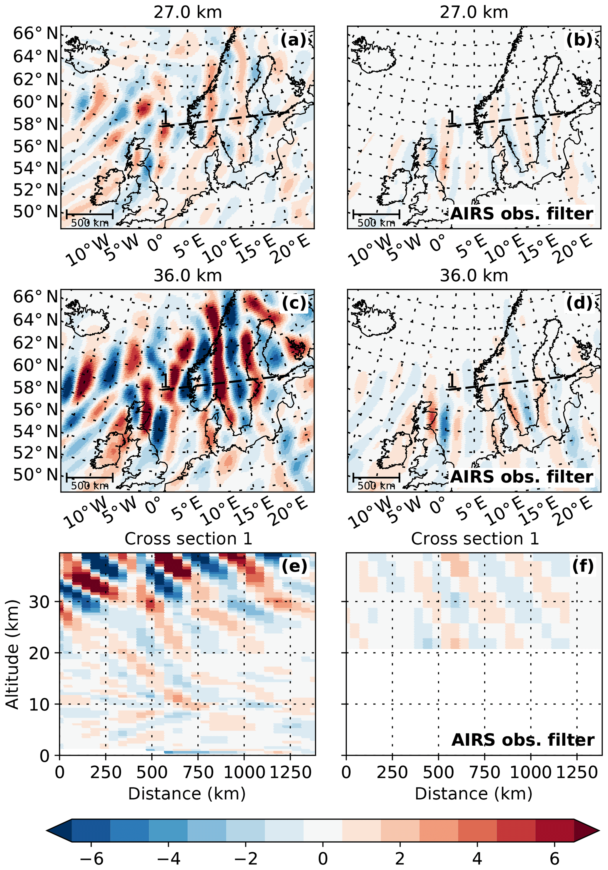
Figure 13ERA5 temperature perturbations for 29 January 2016 03:00 UTC and the influence of the AIRS observational filter. Panels (a), (c), and (e) show the original ERA5 data; panels (b), (d), and (f) show what remains if the model data are convolved with the averaging kernel matrix of the AIRS retrieval shown in Fig. 2a.
A comparison of these simulated AIRS measurements (Fig. 13c and d) with the real AIRS measurements (Fig. 11) shows excellent agreement.
In this paper, a complex gravity wave field above southern Scandinavia was examined with respect to its sources and propagation paths. Measurements taken with GLORIA on 28 January 2016 on two consecutive linear flight legs show a complex wave field, composed of multiple wave packets with different spatial structure, demonstrating the capability of GLORIA limited angle tomography (LAT) to reproduce complex wave patterns. Even though the overall wave structure is similar in both retrievals (one from each flight leg), some difference in wave orientation and the location of small features can be seen. These differences stem from the slight difference in space and time.
A three-dimensional spectral analysis revealed large-scale waves with horizontal wavelengths of around 400 km and vertical wavelengths of between 5 and 7 km. The different vertical wavelengths originate from multiple wave packets in the same analysis field. The different large-scale wave packets were distinguished and characterised by the S3D spectral analysis method.
After subtraction of the large-scale waves, a very complex small-scale wave field with a chequerboard structure remained. Such a chequerboard pattern is an indication of a superposition of at least two wave packets with different propagation directions. An upgrade of the S3D fitting routine is required to properly distinguish and characterise the small-scale wave packets in this chequerboard pattern. Such an upgrade is planned for the near future.
The large-scale wave components were analysed further with the GROGRAT ray tracer and three potential sources were identified: the orography of the Scandes and both a jet-exit region as well as a low-pressure system, which were travelling from west to east over the Atlantic Ocean and southern Scandinavia. The ray traces going back to the orography propagate almost vertically upwards through the GLORIA measurement volume and up into the mid-stratosphere, while the backward ray traces not reaching the mountains originate from west of the Scandinavian Peninsula and cross the mountain wave region from west to east exactly at the GLORIA measurement altitude. Thus, very likely, it is not only the small-scale wave component that consists of multiple wave packets, but the large-scale wave component does, too.
A comparison of one ray trace with ERA5 model data, confirms the prediction of two wave packets crossing each other. According to both models, GROGRAT and ERA5, the two wave packets propagate up to the middle stratosphere. Even though GLORIA and AIRS cover rather different parts of the full gravity wave spectrum, the wave packets observed by GLORIA and propagated forward by GROGRAT can be re-identified in the AIRS measurements: taking into account the different visibility filters of the measurement techniques, the AIRS measurements and the predictions by the ray tracer and ERA5 qualitatively show a high correlation. This is the case despite a strong underestimation of wave amplitudes by AIRS for waves with vertical wavelengths shorter than around 25 km. Furthermore, in agreement with Meyer et al. (2018), we report an overestimation of the vertical wavelengths for the AIRS measurements presented.
In summary, this study demonstrated that LAT using GLORIA is a well-suited tool to observe complex gravity wave fields in 3-D in the UT/LS region and accurately identify several wave components simultaneously. At the same time, such highly resolved 3-D observations challenge the currently existing analysing techniques, e.g. S3D, which will have to be expanded to describe gravity wave interference patterns such as chequerboard patterns in the future. Furthermore, the accuracy of forward and backward ray tracing shown in this study opens new possibilities for combining ray tracing with dedicated 3-D measurements in even more complex situations to gain a better understanding of gravity wave sources and propagation patterns. Last but not least, the example case shows that even in the presence of a prominent mountain ridge, the observed wave patterns can be determined from different sources of comparable strength.
Due to the local nature of GLORIA measurements, global filtering algorithms, as used for model data and satellite instruments, are not suitable for the scale separation of the atmospheric temperature. Furthermore, GLORIA measurements do not have the same spherical latitude–longitude grid as model data. Instead they are sampled to regular Cartesian coordinate systems with kilometre distance to a reference point as x and y coordinates. The reference point is chosen ad hoc for each retrieval separately and is always located somewhere in the centre of the measurement volume. A number of low-pass filters are suitable for the scale separation on regional data sets. To identify the best method for the GLORIA measurements, a 2-D fast Fourier transform (FFT) filter, a running mean filter, a Gaussian filter, an SG filter, and a Butterworth filter (BW filter; Butterworth, 1930) are compared in the following. The separation of pass and stop frequencies are handled differently in each method (Fig. A1). The FFT filter has a very sharp transition from pass to stop band but requires a periodic signal, which GLORIA measurements cannot provide. Assuming the GLORIA measurements to be periodic in space introduces edge effects as can be seen in Fig. A2g–i. The running mean filter and the Gaussian filter both have a very flat transition between pass and stop band. This makes a clear separation more challenging. In contrast, the SG filter as well as the BW filter have a faster transition between pass and stop band.
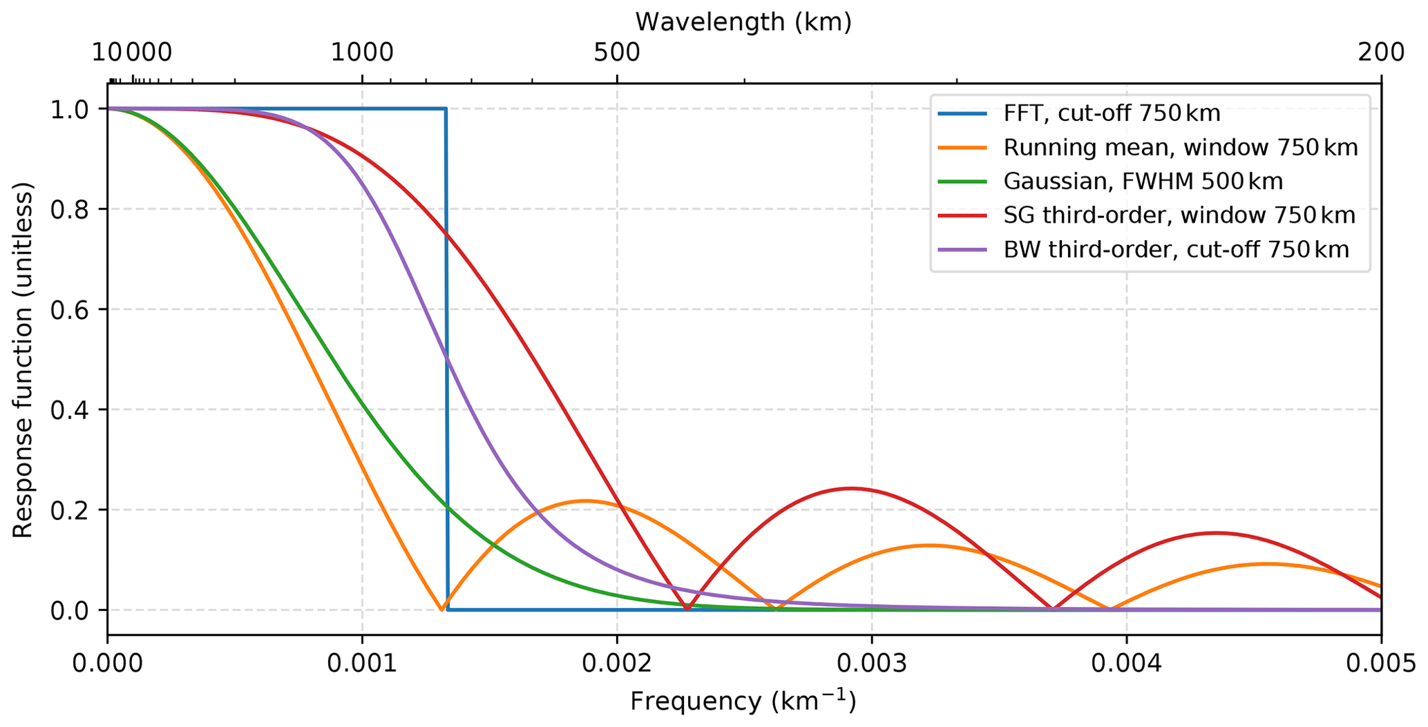
Figure A1Frequency response of different low-pass filters to a delta function in spatial space. Shown are a fast Fourier transform (FFT) with a cut-off wavelength of 750 km, a running mean filter with a window width of 750 km, a Gaussian filter with a full width at half maximum (FWHM) of 500 km, a Savitzky–Golay (SG) third-order polynomial smoothing in running windows of 750 km width, and a third-order Butterworth (BW) filter with a cut-off wavelength of 750 km.

Figure A2Comparison of different scale separation methods applied to a synthetic temperature field. The left column shows horizontal cross sections at 11.5 km altitude, the middle column cross sections in the x–z plane along the y axis, and the right column cross sections in the y–z plane along the x axis. The synthetic temperature (d–f) is constructed from the international standard atmosphere (ISO 2533:1975, 1975), a synoptic-scale zonal wave, and a mesoscale GW (a–c). Detailed descriptions of the different fields and their exact structure can be found in the text. Temperature fluctuations calculated by subtracting the low-pass-filtered background fields from the original synthetic temperature field for different filtering techniques are shown in rows 3–7. A perfect filter should be able to fully reproduce the synthetic GW structure shown in the first row.
Table A1Different filters used for the scale separation of GWs and background and their set-up parameters.

To test these filters systematically on GLORIA-like data, a synthetic temperature field is constructed, which covers an altitude range from 8 to 15 km and has a horizontal extent of 1000 km centred around the coordinate origin (Fig. A2d–f). This temperature field is composed by a superposition of an international standard atmosphere profile (ISO 2533:1975, 1975), a synoptic-scale wave, and a mesoscale GW (Fig. A2a–c). The international standard atmosphere is defined in two altitude ranges: above 11 km, a constant value of 216.15 K is assumed; below 11 km altitude, the temperature decreases with a constant gradient of −6.5 K km−1. As the filtering methods are very sensitive to abrupt changes, a running mean with a 1 km window is applied to the standard atmosphere profile to smooth the transition between the two regimes. The synoptic-scale wave has a wavelength of 1500 km (corresponds to wave number 12 at 60∘ latitude), phase fronts oriented parallel to the y axis, and a temperature amplitude of 1.5 K. The mesoscale GW is chosen to have a horizontal orientation perpendicular to the synoptic-scale wave, a horizontal wavelength of 300 km, and a vertical wavelength of 5 km. The constructed wave is further multiplied by Gaussian functions in all spatial dimensions to simulate the often localised nature of real GW packets. The Gaussian functions have a full width at half maximum (FWHM) of 400 km in both horizontal directions and a FWHM of 5 km in the vertical. The sum of mean temperature, synoptic-scale wave, and GW (Fig. A2d–f) is used as input for the different filtering algorithms.
All filtering algorithms are applied sequentially in both horizontal dimensions to avoid GWs which are oriented along one horizontal axis being erroneously considered as background. The exact set-ups of the different filters are summarised in Table A1. The results are shown in Fig. A2. With the FFT filter (third row), the running mean (fourth row), and the Gaussian filter (fifth row), parts of the synoptic-scale wave remain in the perturbation field. Thus, these filters are not appropriate for the scale separation of GLORIA data. Both the SG filter (sixth row) as well as the BW filter (seventh row) qualitatively reproduce the original GW structure (Fig. A2a–c) with minimal altering effects. The BW filter seems to shift the wave phases outwards, which is likely to be due to a small part of the synoptic-scale wave remaining in the signal. A quantitative comparison is done by calculating the Pearson coefficient P correlating the original wave with the filtered results:
with x1…xn being all data points of the original wave field, the mean of the original wave field, y1…yn all data points of the remaining wave field after filtering, and the mean of the remaining wave field after filtering. The FFT filter reaches a correlation with the original of 53.2 %, the running mean of 51.5 %, the Gaussian of 86.9 %, the SG filter of 99.4 % and the BW filter of 98.5 %. Thus, the Pearson coefficients confirm that the SG filter is the best choice for GLORIA-like measurements. Other orientations and wavelengths of both synoptic-scale waves and GWs have been tested and lead to similar results.
Including an additional filter over the altitude dimension can further help to remove the effects of small-scale weather systems. Thus, for the GLORIA measurements presented in this paper, an additional third-order SG filter with a window length of 3 km is applied in the vertical after the horizontal filtering.
The tomographic retrieval data of GLORIA are available from the HALO database (Krisch and Ungermann, 2020a, b). AIRS retrieval data are available by contacting L. Hoffmann, Forschungszentrum Jülich. The ECMWF operational analysis fields are available directly through ECMWF (ECMWF, 2017), ERA5 fields are available through the Copernicus Climate Data Store (C3S, 2017).
IK, PP, JU, WW, and MR contributed to the GLORIA data acquisition. IK and JU performed the tomographic retrievals; WW, MR, and PP provided scientific support for the GLORIA retrievals. LH developed the AIRS temperature retrieval and provided the AIRS temperature data. IK, ME, PP, CS, and JU developed and optimised the S3D routine. IK and ME performed the sinusoidal fits of GLORIA and AIRS data, respectively. PP and CS were responsible for the GROGRAT calculations. All co-authors contributed to the paper preparation and the interpretation of the results.
The authors declare that they have no conflict of interest.
The authors gratefully acknowledge the computing time granted through JARA on the supercomputer JURECA at Forschungszentrum Jülich (Jülich Supercomputing Centre, 2018). We sincerely thank Anu Dudhia, Oxford University, for providing the Reference Forward Model (RFM) used to calculate the optical path and extinction cross-section tables required by our forward models. Douglas Kinnison, NCAR, is thanked for kindly providing the WACCM4 model data used in the retrieval. The European Centre for Medium-Range Weather Forecasts (ECMWF) is acknowledged for meteorological data support. The results are based on the efforts of all members of the GLORIA team, including the technology institutes ZEA-1 and ZEA-2 at Forschungszentrum Jülich and the Institute for Data Processing and Electronics at the Karlsruhe Institute of Technology. We would also like to thank the pilots and ground-support team at the Flight Experiments facility of the Deutsches Zentrum für Luft- und Raumfahrt (DLR-FX). Manfred Ern would like to acknowledge discussions at the International Space Science Institute (ISSI), Bern, with members of the ISSI team “New Quantitative Constraints on Orographic Gravity Wave Stress and Drag”.
This research has been supported by the Bundesministerium für Bildung und Forschung (grant nos. 01LG1206B and 01LG1206C), the European Space Agency (grant no. 4000115111/15/NL/FF/ah), and the Deutsche Forschungsgemeinschaft (grant no. FOR 1898).
The article processing charges for this open-access
publication were covered by a Research
Centre of the Helmholtz Association.
This paper was edited by Bernd Funke and reviewed by Neil Hindley and one anonymous referee.
Alexander, M. J.: Interpretations of observed climatological patterns in stratospheric gravity wave variance, Geophys. Res. Lett., 103, 8627–8640, https://doi.org/10.1029/97JD03325, 1998. a
Alexander, M. J., Geller, M., McLandress, C., Polavarapu, S., Preusse, P., Sassi, F., Sato, K., Eckermann, S., Ern, M., Hertzog, A., Kawatani, Y., Pulido, M., Shaw, T. A., Sigmond, M., Vincent, R., and Watanabe, S.: Recent developments in gravity-wave effects in climate models and the global distribution of gravity-wave momentum flux from observations and models, Q. J. Roy. Meteorol. Soc., 136, 1103–1124, https://doi.org/10.1002/qj.637, 2010. a, b
Aumann, H. H., Chahine, M. T., Gautier, C., Goldberg, M. D., Kalnay, E., McMillin, L. M., Revercomb, H., Rosenkranz, P. W., Smith, W. L., Staelin, D. H., Strow, L. L., and Susskind, J.: AIRS/AMSU/HSB on the Aqua Mission: Design, Science Objective, Data Products, and Processing Systems, in: IEEE T. Geosci. Remote. Sens., Vol. 41, 253–264, https://doi.org/10.1109/TGRS.2002.808356, 2003. a
Butterworth, S.: On the Theory of Filter Amplifiers, Wireless Engineer, 7, 1930. a
C3S: ERA5: Fifth generation of ECMWF atmospheric reanalyses of the global climate . Copernicus Climate Change Service (C3S) Climate Data Store (CDS), available at: https://cds.climate.copernicus.eu, last access: April 2017. a
Chahine, M. T., Pagano, T. S., Aumann, H. H., Atlas, R., Barnet, C., Blaisdell, J., Chen, L., Divakarla, M., Fetzer, E. J., Goldberg, M., Gautier, C., Granger, S., Hannon, S., Irion, F. W., Kakar, R., Kalnay, E., Lambrigtsen, B. H., Lee, S.-Y., Le Marshall, J., McMillan, W. W., McMillin, L., Olsen, E. T., Revercomb, H., Rosenkranz, P., Smith, W. L., Staelin, D., Strow, L. L., Susskind, J., Tobin, D., Wolf, W., and Zhou, L.: Improving weather forecasting and providing new data on greenhouse gases, B. Am. Meteorol. Soc., 87, 911–926, https://doi.org/10.1175/BAMS-87-7-911, 2006. a
DLR: HALO Website, available at: http://www.halo.dlr.de/aircraft/specifications.html, last access: 17 May 2018. a
Eckermann, S. D. and Marks, C. J.: GROGRAT: a New Model of the Global propagation and Dissipation of Atmospheric Gravity Waves, Adv. Space Res., 20, 1253–1256, 1997. a, b, c
Eckermann, S. D. and Vincent, R. A.: Falling sphere observations of anisotropic gravity wave motions in the upper stratosphere over Australia, Pure Appl. Geophys., 130, 509–532, 1989. a
ECMWF: European Centre for Medium-Range Weather Forecasts (ECMWF) Atmospheric Model high resolution data, available at: https://www.ecmwf.int/en/forecasts/datasets, last access: April 2017. a
Ern, M., Preusse, P., and Warner, C. D.: A comparison between CRISTA satellite data and Warner and McIntyre gravity wave parameterization scheme: horizontal and vertical wavelength filtering of gravity wave momentum flux, Adv. Space Res., 35, 2017–2023, https://doi.org/10.1016/j.asr.2005.04.109, 2005. a
Ern, M., Preusse, P., and Warner, C. D.: Some experimental constraints for spectral parameters used in the Warner and McIntyre gravity wave parameterization scheme, Atmos. Chem. Phys., 6, 4361–4381, https://doi.org/10.5194/acp-6-4361-2006, 2006. a
Ern, M., Hoffmann, L., and Preusse, P.: Directional gravity wave momentum fluxes in the stratosphere derived from high-resolution AIRS temperature data, Geophys. Res. Lett., 44, 475–485, https://doi.org/10.1002/2016GL072007, 2017. a, b
Ern, M., Trinh, Q. T., Preusse, P., Gille, J. C., Mlynczak, M. G., Russell III, J. M., and Riese, M.: GRACILE: a comprehensive climatology of atmospheric gravity wave parameters based on satellite limb soundings, Earth Syst. Sci. Data, 10, 857–892, https://doi.org/10.5194/essd-10-857-2018, 2018. a
Fetzer, E. J. and Gille, J. C.: Gravity wave variance in LIMS temperatures. Part I: Variability and comparison with background winds, J. Atmos. Sci., 51, 2461–2483, https://doi.org/10.1175/1520-0469(1994)051<2461:GWVILT>2.0.CO;2, 1994. a
Friedl-Vallon, F., Gulde, T., Hase, F., Kleinert, A., Kulessa, T., Maucher, G., Neubert, T., Olschewski, F., Piesch, C., Preusse, P., Rongen, H., Sartorius, C., Schneider, H., Schönfeld, A., Tan, V., Bayer, N., Blank, J., Dapp, R., Ebersoldt, A., Fischer, H., Graf, F., Guggenmoser, T., Höpfner, M., Kaufmann, M., Kretschmer, E., Latzko, T., Nordmeyer, H., Oelhaf, H., Orphal, J., Riese, M., Schardt, G., Schillings, J., Sha, M. K., Suminska-Ebersoldt, O., and Ungermann, J.: Instrument concept of the imaging Fourier transform spectrometer GLORIA, Atmos. Meas. Tech., 7, 3565–3577, https://doi.org/10.5194/amt-7-3565-2014, 2014. a, b
Fritts, D. C. and Rastogi, P. K.: Convective and dynamical instabilities due to gravity wave motions in the lower and middle atmosphere: theory and observations, Radio Sci., 20, 1247–1277, 1985. a
Fritts, D. C., Smith, R. B., Taylor, M. J., Doyle, J. D., Eckermann, S. D., Doernbrack, A., Rapp, M., Williams, B. P., Pautet, P. D., Bossert, K., Criddle, N. R., Reynolds, C. A., Reinecke, P. A., Uddstrom, M., Revell, M. J., Turner, R., Kaifler, B., Wagner, J. S., Mixa, T., Kruse, C. G., Nugent, A. D., Watson, C. D., Gisinger, S., Smith, S. M., Lieberman, R. S., Laughman, B., Moore, J. J., Brown, W. O., Haggerty, J. A., Rockwell, A., Stossmeister, G. J., Williams, S. F., Hernandez, G., Murphy, D. J., Klekociuk, A. R., Reid, I. M., and Ma, J.: The Deep Propagating Gravity Wave Experiment (DEEPWAVE): An Airborne and Ground-Based Exploration of Gravity Wave Propagation and Effects from Their Sources throughout the Lower and Middle Atmosphere, B. Am. Meteorol. Soc., 97, 425–453, https://doi.org/10.1175/BAMS-D-14-00269.1, 2016. a
Garcia, R. R., Smith, A. K., Kinnison, D. E., de la Camara, A., and Murphy, D. J.: Modification of the Gravity Wave Parameterization in the Whole Atmosphere Community Climate Model: Motivation and Results, J. Atmos. Sci., 74, 275–291, https://doi.org/10.1175/JAS-D-16-0104.1, 2017. a
Geller, M. A., Alexander, M. J., Love, P. T., Bacmeister, J., Ern, M., Hertzog, A., Manzini, E., Preusse, P., Sato, K., Scaife, A. A., and Zhou, T.: A comparison between gravity wave momentum fluxes in observations and climate models, J. Climate, 26, 6383–6405, https://doi.org/10.1175/JCLI-D-12-00545.1, 2013. a
Giez, A.: Effective Test and Calibration of a Trailing Cone System on the Atmospheric Research Aircraft HALO, Proceedings of the 56th Annual Symposium of the Society of Experimental Test Pilots, Anaheim, USA, 2012. a
Gisinger, S., Wagner, J., and Witschas, B.: Airborne measurements and large-eddy simulations of small-scale gravity waves at the tropopause inversion layer over Scandinavia, Atmos. Chem. Phys., 20, 10091–10109, https://doi.org/10.5194/acp-20-10091-2020, 2020. a, b
Guest, F., Reeder, M., Marks, C., and Karoly, D.: Inertia-gravity waves observed in the lower stratosphere over Macquarie Island, J. Atmos. Sci., 57, 737–752, 2000. a
Hertzog, A., Boccara, G., Vincent, R. A., Vial, F., and Cocquerez, P.: Estimation of gravity wave momentum flux and phase speeds from quasi-Lagrangian stratospheric balloon flights. Part II: Results from the Vorcore campaign in Antarctica, J. Atmos. Sci., 65, 3056–3070, https://doi.org/10.1175/2008JAS2710.1, 2008. a
Hindley, N. P., Wright, C. J., Smith, N. D., Hoffmann, L., Holt, L. A., Alexander, M. J., Moffat-Griffin, T., and Mitchell, N. J.: Gravity waves in the winter stratosphere over the Southern Ocean: high-resolution satellite observations and 3-D spectral analysis, Atmos. Chem. Phys., 19, 15377–15414, https://doi.org/10.5194/acp-19-15377-2019, 2019. a
Hoffmann, L. and Alexander, M. J.: Retrieval of stratospheric temperatures from Atmospheric Infrared Sounder radiance measurements for gravity wave studies, J. Geophys. Res., 114, D07105, https://doi.org/10.1029/2008JD011241, 2009. a, b, c
ISO 2533:1975: Standard Atmosphere, Standard, International Organization for Standardization, Geneva, CH, 1975. a, b
Jülich Supercomputing Centre: JURECA: Modular supercomputer at Jülich Supercomputing Centre, J. Large-Scale Res. Facil., 4, A132, https://doi.org/10.17815/jlsrf-4-121-1, 2018. a
Krasauskas, L., Ungermann, J., Ensmann, S., Krisch, I., Kretschmer, E., Preusse, P., and Riese, M.: 3-D tomographic limb sounder retrieval techniques: irregular grids and Laplacian regularisation, Atmos. Meas. Tech., 12, 853–872, https://doi.org/10.5194/amt-12-853-2019, 2019. a
Krisch, I. and Ungermann, J.: 2016-01-28_db_north-leg.nc, availble at: https://halo-db.pa.op.dlr.de/dataset/6856, last access: 11 March 2020a. a
Krisch, I. and Ungermann, J.: 2016-01-28_db_south-leg.nc, available at: https://halo-db.pa.op.dlr.de/dataset/6857, last access: 11 March 2020b. a
Krisch, I., Preusse, P., Ungermann, J., Dörnbrack, A., Eckermann, S. D., Ern, M., Friedl-Vallon, F., Kaufmann, M., Oelhaf, H., Rapp, M., Strube, C., and Riese, M.: First tomographic observations of gravity waves by the infrared limb imager GLORIA, Atmos. Chem. Phys., 17, 14937–14953, https://doi.org/10.5194/acp-17-14937-2017, 2017. a, b, c, d, e
Krisch, I., Ungermann, J., Preusse, P., Kretschmer, E., and Riese, M.: Limited angle tomography of mesoscale gravity waves by the infrared limb-sounder GLORIA, Atmos. Meas. Tech., 11, 4327–4344, https://doi.org/10.5194/amt-11-4327-2018, 2018. a, b, c, d, e
Lehmann, C. I., Kim, Y.-H., Preusse, P., Chun, H.-Y., Ern, M., and Kim, S.-Y.: Consistency between Fourier transform and small-volume few-wave decomposition for spectral and spatial variability of gravity waves above a typhoon, Atmos. Meas. Tech., 5, 1637–1651, https://doi.org/10.5194/amt-5-1637-2012, 2012. a, b
Marks, C. J. and Eckermann, S. D.: A Three-Dimensional Nonhydrostatic Ray-Tracing Model for Gravity Waves: Formulation and Preliminary Results for the Middle Atmosphere, J. Atmos. Sci., 52, 1959–1984, https://doi.org/10.1175/1520-0469(1995)052<1959:ATDNRT>2.0.CO;2, 1995. a, b, c
McLandress, C., Shepherd, T. G., Polavarapu, S., and Beagley, S. R.: Is Missing Orographic Gravity Wave Drag near 60 degrees S the Cause of the Stratospheric Zonal Wind Biases in Chemistry Climate Models?, J. Atmos. Sci., 69, 802–818, https://doi.org/10.1175/JAS-D-11-0159.1, 2012. a
Meyer, C. and Hoffmann, L.: Validation of AIRS high-resolution stratospheric temperature retrievals, in: Proc. SPIE, Vol. 9242, 92420L, SPIE Remote Sensing Europe, Amsterdam (Netherlands), 22–25 Sep 2014, https://doi.org/10.1117/12.2066967, 2014. a
Meyer, C. I., Ern, M., Hoffmann, L., Trinh, Q. T., and Alexander, M. J.: Intercomparison of AIRS and HIRDLS stratospheric gravity wave observations, Atmos. Meas. Tech., 11, 215–232, https://doi.org/10.5194/amt-11-215-2018, 2018. a, b, c
Nappo, C. J.: An Introduction to Atmospheric Gravity Waves, Academic Press, 2nd Edn., 2012. a
Oelhaf, H., Sinnhuber, B.-M., Woiwode, W., Bönisch, H., Bozem, H., Engel, A., Fix, A., Friedl-Vallon, F., Grooß, J.-U., Hoor, P., Johansson, S., Jurkat-Witschas, T., Kaufmann, S., Krämer, M., Krause, J., Kretschmer, E., Lörks, D., Marsing, A., Orphal, J., Pfeilsticker, K., Pitts, M., Poole, L., Preusse, P., Rapp, M., Riese, M., Rolf, C., Ungermann, J., Voigt, C., Volk, C. M., Wirth, M., Zahn, A., and Ziereis, H.: POLSTRACC: Airborne experiment for studying the Polar Stratosphere in a Changing Climate with the high-altitude long-range research aircraft HALO, B. Am. Meteorol. Soc., 100, 2634–2664, https://doi.org/10.1175/BAMS-D-18-0181.1, 2019. a
Pitteway, M. L. V. and Hines, C. O.: The viscous damping of atmospheric gravity waves, Can. J. Phys., 41, 1935–1948, https://doi.org/10.1139/p63-194, 1963. a
Plougonven, R. and Zhang, F.: Internal gravity waves from atmospheric jets and fronts, Rev. Geophys., 52, 33–76, https://doi.org/10.1002/2012RG000419, 2014. a
Portele, T. C., Dörnbrack, A., Wagner, J. S., Gisinger, S., Ehard, B., Pautet, P.-D., and Rapp, M.: Mountain-Wave Propagation under Transient Tropospheric Forcing: A DEEPWAVE Case Study, Mon. Weather Rev., 146, 1861–1888, https://doi.org/10.1175/MWR-D-17-0080.1, 2018. a
Preusse, P., Eckermann, S. D., and Offermann, D.: Comparison of global distributions of zonal-mean gravity wave variance inferred from different satellite instruments, Geophys. Res. Lett., 27, 3877–3880, https://doi.org/10.1029/2000GL011916, 2000. a
Preusse, P., Ern, M., Bechtold, P., Eckermann, S. D., Kalisch, S., Trinh, Q. T., and Riese, M.: Characteristics of gravity waves resolved by ECMWF, Atmos. Chem. Phys., 14, 10483–10508, https://doi.org/10.5194/acp-14-10483-2014, 2014. a, b
Rabier, F., Mahfouf, J.-F., Fisher, M., Järvinen, H., Simmons, A., Andersson, E., Bouttier, F., Courtier, P., Hamrud, M., Haseler, J., Hollingsworth, A., Isaksen, L., Klinker, E., Saarinen, S., Temperton, C., Thépaut, J.-N., Undén, P., and Vasiljevic, D.: Recent experimentation on 4D-Var and first results from a Simplified Kalman Filter, ECMWF technical memoranda, No. 240, published by ECMWF, Shinfield Park, Reading, https://doi.org/10.21957/rxpcc3rzv, 1997. a
Riese, M., Oelhaf, H., Preusse, P., Blank, J., Ern, M., Friedl-Vallon, F., Fischer, H., Guggenmoser, T., Höpfner, M., Hoor, P., Kaufmann, M., Orphal, J., Plöger, F., Spang, R., Suminska-Ebersoldt, O., Ungermann, J., Vogel, B., and Woiwode, W.: Gimballed Limb Observer for Radiance Imaging of the Atmosphere (GLORIA) scientific objectives, Atmos. Meas. Tech., 7, 1915–1928, https://doi.org/10.5194/amt-7-1915-2014, 2014. a, b
Sandu, I., Bechtold, P., Beljaars, A., Bozzo, A., Pithan, F., Shepherd, T. G., and Zadra, A.: Impacts of parameterized orographic drag on the Northern Hemisphere winter circulation, J. Adv. Model. Earth Syst., 8, 196–211, https://doi.org/10.1002/2015MS000564, 2016. a
Savitzky, A. and Golay, M. J. E.: Smoothing and Differentiation of Data by Simplified Least Squares Procedures, Anal. Chem., 36, 1627–1639, https://doi.org/10.1021/ac60214a047, 1964. a
Schoon, L. and Zülicke, C.: A novel method for the extraction of local gravity wave parameters from gridded three-dimensional data: description, validation, and application, Atmos. Chem. Phys., 18, 6971–6983, https://doi.org/10.5194/acp-18-6971-2018, 2018. a
Shepherd, T. G.: Atmospheric circulation as a source of uncertainty in climate change projections, Nat. Geosci., 7, 703–708, https://doi.org/10.1038/NGEO2253, 2014. a
Sigmond, M. and Scinocca, J. F.: The Influence of the Basic State on the Northern Hemisphere Circulation Response to Climate Change, J. Climate, 23, 1434–1446, https://doi.org/10.1175/2009JCLI3167.1, 2010. a
Skamarock, W. C.: Evaluating mesoscale NWP models using kinetic energy spectra, Mon. Weather Rev., 132, 3019–3032, 2004. a
Smith, R. B. and Kruse, C. G.: Broad-Spectrum Mountain Waves, Journal of the Atmospheric Sciences, 74, 1381–1402, https://doi.org/10.1175/JAS-D-16-0297.1, 2017. a
Smith, R. B., Nugent, A. D., Kruse, C. G., Fritts, D. C., Doyle, J. D., Eckermann, S. D., Taylor, M. J., Doernbrack, A., Uddstrom, M., Cooper, W., Romashkin, P., Jensen, J., and Beaton, S.: Stratospheric Gravity Wave Fluxes and Scales during DEEPWAVE, J. Atmos. Sci., 73, 2851–2869, https://doi.org/10.1175/JAS-D-15-0324.1, 2016. a
Strube, C., Ern, M., Preusse, P., and Riese, M.: Removing spurious inertial instability signals from gravity wave temperature perturbations using spectral filtering methods, Atmos. Meas. Tech. Discuss., https://doi.org/10.5194/amt-2020-29, in review, 2020. a
Trey, F.: Ein Beitrag zum Studium der Luftwogen, Meteorol. Z., 36, 25–28, 1919. a
Trinh, Q. T., Kalisch, S., Preusse, P., Ern, M., Chun, H.-Y., Eckermann, S. D., Kang, M.-J., and Riese, M.: Tuning of a convective gravity wave source scheme based on HIRDLS observations, Atmos. Chem. Phys., 16, 7335–7356, https://doi.org/10.5194/acp-16-7335-2016, 2016. a
Ungermann, J., Blank, J., Lotz, J., Leppkes, K., Hoffmann, L., Guggenmoser, T., Kaufmann, M., Preusse, P., Naumann, U., and Riese, M.: A 3-D tomographic retrieval approach with advection compensation for the air-borne limb-imager GLORIA, Atmos. Meas. Tech., 4, 2509–2529, https://doi.org/10.5194/amt-4-2509-2011, 2011. a
Vosper, S. and Ross, A.: Sampling Errors in Observed Gravity Wave Momentum Fluxes from Vertical and Tilted Profiles, Atmosphere, 11, 57, https://doi.org/10.3390/atmos11010057, 2020. a
Wang, L. and Geller, M. A.: Morphology of gravity-wave energy as observed from 4 years (1998–2001) of high vertical resolution U.S. radiosonde data, J. Geophys. Res., 108, D16, https://doi.org/10.1029/2002JD002786, 2003. a
Wegener, A.: Studien über Luftwogen, Beitr. Physik Freien Atmos., 4, 23–25, 1906. a
Wright, C. J., Hindley, N. P., Hoffmann, L., Alexander, M. J., and Mitchell, N. J.: Exploring gravity wave characteristics in 3-D using a novel S-transform technique: AIRS/Aqua measurements over the Southern Andes and Drake Passage, Atmos. Chem. Phys., 17, 8553–8575, https://doi.org/10.5194/acp-17-8553-2017, 2017. a, b
Zhang, S. D., Huang, C. M., Huang, K. M., Yi, F., Zhang, Y. H., Gong, Y., and Gan, Q.: Spatial and seasonal variability of medium- and high-frequency gravity waves in the lower atmosphere revealed by US radiosonde data, Ann. Geophys., 32, 1129–1143, https://doi.org/10.5194/angeo-32-1129-2014, 2014. a
Zhu, X.: A New Theory of the Saturated Gravity Wave Spectrum for the Middle Atmosphere, J. Atmos. Sci., 51, 3615–3626, https://doi.org/10.1175/1520-0469(1994)051<3615:ANTOTS>2.0.CO;2, 1994. a
- Abstract
- Introduction
- Methodology and data description
- Data acquisition and measurement results
- Analysis and discussion
- Conclusions
- Appendix A: Comparison of different scale separation methods for GLORIA measurements
- Data availability
- Author contributions
- Competing interests
- Acknowledgements
- Financial support
- Review statement
- References