Effects of global ship emissions on European air pollution levels

Ship emissions constitute a large, and so far poorly regulated, source of air pollution. Emissions are mainly clustered along major ship routes both in open seas and close to densely populated shorelines. Major air pollutants emitted include sulfur dioxide, NO_x, and primary particles. Sulfur and NO_x are both major contributors to the formation of secondary fine particles (PM_2.5) and to acidification and eutrophication. In addition, NO_x is a major precursor for ground-level ozone. In this paper, we quantify the contributions from international shipping to European air pollution levels and depositions.

This study is based on global and regional model calculations. The model runs are made with meteorology and emission data representative of the year 2017 after the tightening of the SECA (sulfur emission control area) regulations in 2015 but before the global sulfur cap that came into force in 2020. The ship emissions have been derived using ship positioning data. We have also made model runs reducing sulfur emissions by 80 % corresponding to the 2020 requirements. This study is based on model sensitivity studies perturbing emissions from different sea areas: the northern European SECA in the North Sea and the Baltic Sea, the Mediterranean Sea and the Black Sea, the Atlantic Ocean close to Europe, shipping in the rest of the world, and finally all global ship emissions together. Sensitivity studies have also been made setting lower bounds on the effects of ship plumes on ozone formation.

Both global- and regional-scale calculations show that for PM_2.5 and depositions of oxidised nitrogen and sulfur, the effects of ship emissions are much larger when emissions occur close to the shore than at open seas. In many coastal countries, calculations show that shipping is responsible for 10 % or more of the controllable PM_2.5 concentrations and depositions of oxidised nitrogen and sulfur. With few exceptions, the results from the global and regional calculations are similar. Our calculations show that substantial reductions in the contributions from ship emissions to PM_2.5 concentrations and to depositions of sulfur can be expected in European coastal regions as a result of the implementation of a 0.5 % worldwide limit of the sulfur content in marine fuels from 2020. For countries bordering the North Sea and Baltic Sea SECA, low sulfur emissions have already resulted in marked reductions in PM_2.5 from shipping before 2020.

For ozone, the lifetime in the atmosphere is much longer than for PM_2.5, and the potential for ozone formation is much larger in otherwise pristine environments. We calculate considerable contributions from open sea shipping. As a result, we find that the largest contributions to ozone in several regions and countries in Europe are from sea areas well outside European waters.

1 Introduction

As shown by both model calculations and measurements, concentrations of almost all air pollutants have decreased throughout most of Europe since 1990 (Colette et al., 2016, 2017). Over the same time span, depositions of eutrophying and in particular acidifying species have also decreased (Theobald et al., 2019). These trends are, with the partial exception of ground level ozone, almost entirely driven by reductions in European land-based emissions (Colette et al., 2016). Since the year 2000, European emission trends are diverse with general downward trends in western European countries and upward trends in eastern Europe (Gaisbauer et al., 2019). The latter upward trends are largely driven by an economic recovery in former Soviet Union states. Emissions from international shipping to the air, relevant in the context of air pollution and depositions in Europe, include PPM (primary particulate matter), sulfur, NO_x, CO, and NMVOC (non-methane volatile organic carbon). Trends in emissions from shipping are less certain than for land-based emissions and differ depending on species and sea area. In general, emissions from shipping have changed less than land-based emissions in western Europe (Gaisbauer et al., 2019), and, as a result, the relative contributions of ship emissions to air pollution and depositions in western parts of Europe have increased. One notable exception is the SECA (sulfur emission control area) regions in the Baltic Sea and the North Sea where sulfur emissions have dropped by more than 1 order of magnitude in the last decade. In the SECAs, the maximum allowed sulfur content in fuels, and consequently the emissions from shipping, has been reduced in several steps with the latest, and most significant, measure implemented in January 2015 that reduced the maximum allowed sulfur content in marine fuels from 1 % to 0.1 % (IMO, 2008). Fuels with higher sulfur content may be used in combination with technology reducing sulfur emission to levels equivalent to the use of low-sulfur fuels. In addition, the EU sulfur directive requires ships to use fuel with 0.1  % sulfur in EU harbour areas. From 2020, a global cap on sulfur content in marine fuels of 0.5 % has been implemented as opposed to an average of about 2.5  % prior to 2020.

The global effects of international shipping on air pollution and depositions have already been identified in several papers (Corbett et al., 2007; Endresen et al., 2003; Eyring et al., 2007; Sofiev et al., 2018). In a global model calculation, Jonson et al. (2018a) found that a large portion of the anthropogenic contributions to PM_2.5 and depositions of sulfur and nitrogen in European coastal regions can be attributed to ship emissions in nearby sea areas. For boundary layer ozone, the same study showed a mixed result with overall percentage contributions to ozone of anthropogenic origin of more than 20 % in several Mediterranean countries and negative contributions in some countries bordering the North Sea caused by ozone titration. In Jonson et al. (2018b), the effects of pollution from other continents, including also the effects of international shipping on European air pollution, were investigated within the framework of TF_HTAP2 (Task Force on Hemispheric Transport of Air Pollution, phase II; http://www.htap.org/, last access: 7 July 2020). These calculations indicated that more than 10 % of the ozone in Europe of anthropogenic origin can be attributed to international shipping. The percentage contributions were similar for both annually averaged ozone and ozone indicators such as SOMO35¹ and POD₁ (deciduous) forest².

In Karl et al. (2019), the EMEP (https://emep.int/mscw/mscw_models.html (last access: September 2020) model, along with two other models, was applied in a regional study on the effects of ship emissions in the Baltic Sea region using meteorology and emissions for the year 2012. In that study, the average contribution of ships to levels of PM_2.5 ranged from 4.15 % to 6.5 % in the entire Baltic Sea region and from 3.15 % to 5.7 % in the coastal land areas. In addition, the model results were compared to measurements in the region. Jonson et al. (2019) found that the implementation of stricter SECA regulations in the Baltic Sea and the North Sea from 2015 resulted in marked reductions in PM_2.5 levels in the Baltic Sea region. In a companion paper using the same data, Barregård et al. (2019) estimated that the number of premature deaths from shipping dropped by one-third between 2014 and 2016.

With ship emissions representative for the year 2013, Lv et al. (2018) calculated contributions from ship emissions to PM_2.5 concentrations of up to 5.2 µg m⁻³ in coastal regions of China, higher than in European coastal regions. Since 2013, emission controls have been imposed in China in several steps limiting the fuel sulfur content in marine fuels to 0.5 % in several Chinese ports and territorial waters.

In this paper, we study the effects of global international shipping further by performing a series of scenario calculations perturbing ship emissions, both globally and from individual sea areas, to attribute the effects of ship emissions on European countries from different sea areas. We have limited the study to air concentrations of PM_2.5 and ozone and to depositions of oxidised nitrogen and sulfur. The calculations are made with meteorology and emissions for the year 2017, but calculations are also made for 2020 and beyond by scaling sulfur emissions outside the North Sea and Baltic Sea SECAs by 0.5 to 2.5 (a decrease in the sulfur content in marine fuels from about 2.5 % to 0.5 %), reflecting the expected reductions in sulfur emissions following the CAP2020 regulations implemented in 2020 (see http://www.imo.org/en/mediacentre/hottopics/pages/sulphur-2020.aspx, last access: 7 July 2020).

The global model calculations are compared to the regional-scale source receptor calculations also for the year 2017 included in the latest EMEP report (EMEP Status Report 1/2019, 2019).

Finally, sensitivity tests have been made to give bounds for the effect of chemistry within exhaust plumes. In pristine environments, pollutant concentrations can be orders of magnitude higher within ship plumes than in their surroundings, whereas in the model these emission plumes are instantly diluted into a large grid volume. Ignoring the chemistry within the plumes can potentially result in an overestimation of ozone.

2 Model description

Concentrations of air pollutants and depositions of sulfur and nitrogen have been calculated with the EMEP Meteorological Synthesising Centre West (MSC-W) model version rv4.34 (hereafter “EMEP model”) on a global model domain with a $\mathrm{0.5}{}^{\circ }\times \mathrm{0.5}{}^{\circ }$ latitude–longitude resolution. The EMEP model is a comprehensive air quality model which has been used extensively during the last four decades for air pollution research and to underpin international air quality legislation. It takes into account processes of emissions, advection, turbulent diffusion, chemical transformations, and wet and dry depositions. The calculations of dry depositions are made separately for each sub-grid land-cover classification. These sub-grid estimates are aggregated to provide output deposition estimates for broader ecosystem categories as deciduous and coniferous forests. A detailed description of the EMEP model can be found in Simpson et al. (2012) with later model updates being described in Simpson et al. (2019) and references therein. The EMEP model is open source (see https://github.com/metno/emep-ctm), last access: 7 July 2020.

For comparison, we also include results from the regional model calculations contained in the latest EMEP report (EMEP Status Report 1/2019, 2019) covering the geographical area between 30 and 82^∘ N and 30^∘ W and 90^∘ E on a $\mathrm{0.3}{}^{\circ }\times \mathrm{0.2}{}^{\circ }$ latitude–longitude resolution. Both the global and regional calculations have been made using 2017 meteorological input data and 2017 emissions. The meteorological input data are from the European Centre for Medium-Range Weather Forecasts (ECMWF) based on the CY40R1 version of their IFS (Integrated Forecast System) model.

2.1 Model evaluation and comparisons to other models

The EMEP model is under continuous development and undergoes extensive evaluation against measurements every year as part of the EMEP status reports (see Gauss et al., 2017, 2018, 2019, for evaluations of the latest emission years available for 2015, 2016, and 2017). The model is also evaluated daily and openly within the Copernicus Atmosphere Monitoring Service, where it is used operationally for regional air quality forecasts and analyses (see https://www.regional.atmosphere.copernicus.eu/, last access: 7 July 2020). In addition, the EMEP regional model has successfully participated in model inter-comparisons and model evaluations in a number of peer-reviewed publications (Colette et al., 2011, 2012; Angelbratt et al., 2011; Dore et al., 2015). In Vivanco et al. (2018), depositions of sulfur and nitrogen species in Europe calculated by 14 regional models were evaluated against measurements showing good results for the EMEP model. In global mode, the model has also participated in a number of model inter-comparisons and model evaluations (Stjern et al., 2016; Tan et al., 2018; Liang et al., 2018; Jonson et al., 2018a). At least for background sites, the performance is comparable for regional and global model applications.

In Karl et al. (2019), the EMEP model, the System for Integrated modeLling of Atmospheric coMposition (SILAM) model, and the Community Multiscale Air Quality Modelling System (CMAQ) model were compared to measurements and in terms of calculated effects of ship emissions in the Baltic Sea. For PM_2.5, both the CMAQ and the EMEP models had a slightly negative bias, whereas the SILAM model had virtually no bias. Even so, the SILAM model calculated a slightly lower contribution from Baltic Sea shipping compared to the other two models. All three models overpredicted ozone for urban measurement sites. The EMEP model also had a moderate positive bias at rural sites. The EMEP model calculated less ozone titration in the shipping lanes most likely as a result of its coarser model resolution compared to the other two models. Over land, all three models calculated small increases in ozone due to ship emissions. In Jonson et al. (2019), the importance of ship emissions was demonstrated by comparing model results and Baltic Sea coastal measurements for 2016 of PM_2.5, SO₂, NO₂, and ozone. Furthermore, the EMEP model had a negative bias for PM_2.5. NO₂ concentrations were severely underestimated when ship emissions were set to 0, illustrating the importance of ship emissions in the real atmosphere. Likewise, 2016 SO₂ concentrations were strongly overestimated when using 2014 emissions.

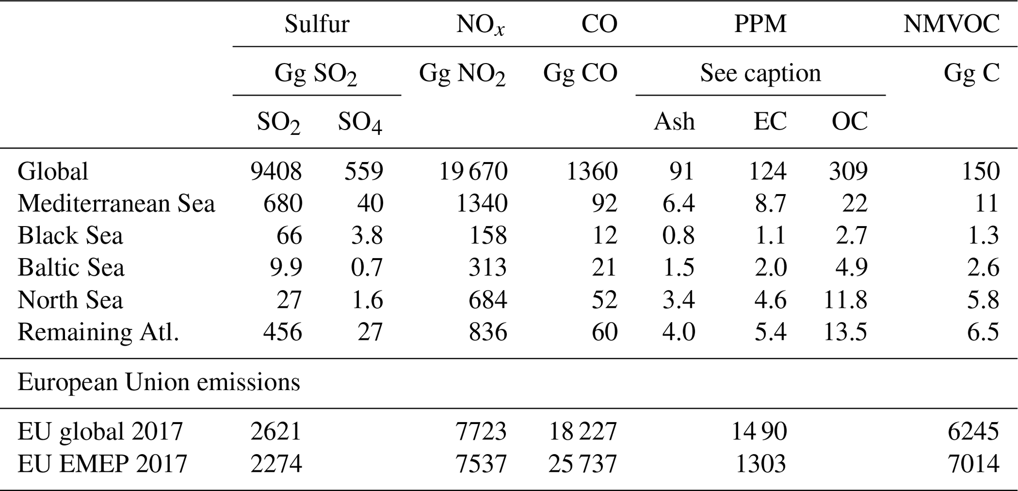
Table 1 Ship emissions from the Finnish Meteorological Institute (FMI) in European sub-sea areas. Sulfur emissions are given as SO₂. PPM emissions are sub-divided into ash, EC (elemental carbon), and OC (organic carbon), all assumed to be emitted as PM_2.5. Total EU emissions used in global and regional calculations are also listed. A total of 5 % of these SO₂ emissions are assumed to be emitted as SO₄.

2.2 Emissions

For the global calculations, land-based emissions have been provided by the International Institute for Applied Systems Analysis (IIASA) within the European FP7 project ECLIPSE (http://www.iiasa.ac.at/web/home/research/researchPrograms/air/ECLIPSEv5.html, last access: July 2020). In this study, we use ECLIPSE version 6a (hereafter referred to as “ECLIPSEv6a”), which is a global emission data set on 0.5^∘×0.5^∘ resolution and is widely used by the scientific community. Some of the methods used in ECLIPSE are described in the recent publication of Höglund-Isaksson et al. (2020). Historical data rely on statistical data (until 2015) for energy from the International Energy Agency (IEA), agricultural data from the United Nations Food and Agriculture Organisation (FAO), the International Fertiliser Association (IFA), additional data for mineral industries from the United States Geological Survey (USGS), and numerous additional sources for informal industries (e.g. brick making, waste, etc.). Current baseline projections rely on the New Policies Scenario (NPS) from the World Energy Outlook 2018 of the IEA (IEA, 2018) FAO projections and for EU agriculture also on the European-wide farm-type model in CAPRI (Common Agricultural Policy Regional Impact). ECLIPSEv6a emissions are available in 5-year intervals from 2005 onward. In this study, the emissions are interpolated to 2017.

The land-based emissions used in the regional model calculations are described in Gaisbauer et al. (2019) and are mainly based on the officially reported data from the countries. In Table 1, these officially reported emissions are listed aggregately for the EU27 countries compared to the ECLIPSEv6a emissions. Differences are of similar magnitude for the individual EU countries. The most significant difference is for sulfur, for which the ECLIPSEv6a emissions are of the order of 15 % higher than those reported to EMEP.

Ship emission data sets used in both the global and regional model calculations are originally from the Finish Meteorological Institute, and they are based on Automatic Identification System (AIS) data processed in the STEAM model (Johansson et al., 2017) and downloaded from the Emissions of atmospheric Compounds and Compilation of Ancillary Data (ECCAD) database (https://eccad.aeris-data.fr/, last access: 7 July 2020). Ship emissions of various species, based on the global data set, are listed in Table 1 separately for the Baltic Sea, the North Sea (including the English Channel), the Mediterranean Sea, and the Black Sea. In addition, emissions are listed for the remaining Atlantic area outside Europe but bounded by 30–82^∘ N and 30^∘ W–90^∘ E, corresponding to the north-east Atlantic Ocean also included in the regional calculations. These three sea areas are depicted in Fig. 1. Finally, emissions are also listed for the total global sea area. Annual ship emissions used in the regional model calculations are based on the same source (Gaisbauer et al., 2019). Even so, total ship emissions in the sea areas as used in the global calculations are somewhat higher than in the regional calculations (see Appendix B in EMEP Status Report 1/2019, 2019, for comparison).

Figure 1 The individual sea areas are marked in red. Shipping emissions in all other sea areas are classified as ROW (rest of world) shipping.

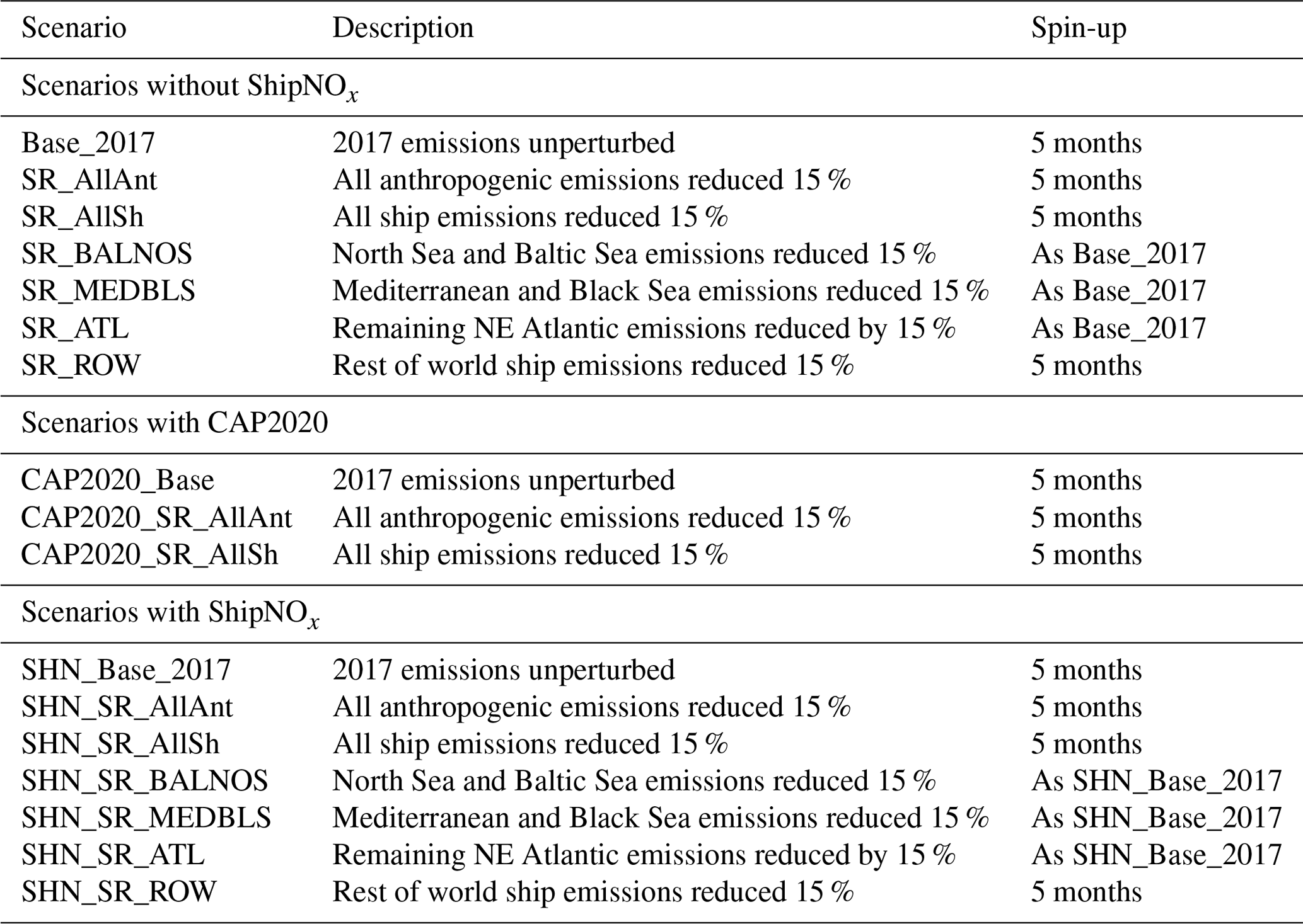
Table 2 Overview of model scenarios used. Separate model spin-up was only performed for Base model run(s) and for model runs with globally perturbed emissions. For SR (source receptor) model runs perturbing limited areas, we use the same spin-up as for the Base runs. CAP2020 emissions are estimated by scaling the emissions outside the North Sea and Baltic Sea SECAs from an assumed pre-CAP2020 global average sulfur content of 2.5 % to 0.5 %. Additional information about the model scenarios is given in Sect. 2.3.

In the FMI emission data, all PPM emissions are assumed to be emitted as PM_2.5. Emissions from leisure boats are not included. In a separate study, Johansson et al. (2020) have quantified the emissions from leisure boats in the Baltic Sea only. Compared to emissions from the commercial fleet, these emissions were insignificant for NO_x and PPMs. However, in regard to emissions of NMVOC, the study concluded that these can be significantly larger from leisure boats than from registered vessels in the Baltic Sea, especially during summer (about 500 % larger). However, as shown in Table 1, the NMVOC to NO_x ratio is close to 1 for land-based emissions but very low for ship emissions.

2.3 Definition of the model sensitivity tests

In order to calculate the effects of ship emissions on air pollution and depositions in Europe, we use a similar approach as in the SR (source receptor) calculations within the EMEP programme (see Appendix C in EMEP Status Report 1/2019, 2019, as the latest example). We reduce the emissions by 15 % in the sea areas in order to make the results comparable to the regional EMEP SR results. Both the global and regional model runs are made for a full calendar year (2017). As some of the species have a long lifetime in the atmosphere (1 month or more), the global model runs are preceded by a 5-month spin-up, but for model runs perturbing only a limited sea area, the spin-up from the Base model run is used (see Table 2). Whereas in the regional EMEP SR calculations emissions of different species are reduced in separate perturbation runs, we in the global runs reduce the emissions of all species simultaneously in the same perturbation run, reducing the number of model runs to one for each of the model scenarios listed in Table 2. We have combined the North Sea and the Baltic Sea into one scenario run because they are both designated as SECAs. Likewise we have combined the Mediterranean Sea and the Black Sea. The sea areas are shown in Fig. 1. ROW (rest of world) is all sea areas not included in the sea areas listed above. We have also made additional model runs with sulfur emissions from ships reduced to CAP2020 levels.

In the interpretation of the model results below, we let the difference between the Base_2017 and the SR_AllAnt model runs (see Table 2) represent 100 % of the effects of all anthropogenic, and thus controllable, global emissions. Similarly we calculate the contributions from global shipping as a whole, or from shipping in a specific area, by subtracting the scenario run for shipping as a whole or from a specific sea area from the Base model run. In this way, we can relate the effects of ship emissions in different regions to the total anthropogenic contribution. Even though not linear, this is a widely used approach that, in addition to in the EMEP reporting, was also taken in the TF_HTAP phase II modelling exercise (see work plan under http://www.htap.org/, last access: 7 July 2020). Reducing the emissions by a different percentage would give slightly different results depending on the species and location. The choice of 15 % is partly political as reductions of this magnitude are achievable within a time frame of a few years and at the same time they give a large enough signal when processing the model output.

For all depositions and air concentrations except ozone (and ozone metrics), we add up the SR runs for the individual sea areas (SR_BALNOS, SR_MEDBLS, SR_ATL, and SR_ROW) and compare with the SR_AllSh emission perturbation which provides a measure of the linearity in the calculations.

In the model calculations described above, the ship emissions are instantly diluted throughout the model grid cells in which the emissions occur. Previous studies (Vinken et al., 2011; Huszar et al., 2010) have shown that this can lead to an overestimation of the ozone formation, in particular in sea areas where NO_x concentrations are otherwise low. The EMEP model has an option for splitting 50 % of the NO_x emissions from shipping into a pseudo-species “ShipNO_x”, and the other half emitted as NO and NO₂, as in the Base model runs (see Simpson et al., 2015). ShipNO_x deposits as NO₂ but undergoes simple atmospheric reactions:

$$\begin{array}{}\text{(R1)}& {\displaystyle }& {\displaystyle }{\mathrm{ShipNO}}_x+\mathrm{OH}\Rightarrow {\mathrm{HNO}}_{\mathrm{3}},\text{(R2)}& {\displaystyle }& {\displaystyle }{\mathrm{ShipNO}}_x\Rightarrow {\mathrm{HNO}}_{\mathrm{3}}.\end{array}$$

Reaction (R1) proceeds with the same rate as the normal NO₂+OH reaction, thus proceeding faster in daylight and in high-OH areas. Reaction (R2) provides a minimum half-life of about 6 h, loosely based upon results shown in Vinken et al. (2011). We have repeated the calculations for the scenarios listed above with the ShipNO_x reactions included. We then assume that the calculations with and without the ShipNO_x split represent a lower and an upper limit of the effects of NO_x emissions from shipping on the formation of ozone both globally and in the individual sea areas.

3 Model results

In this section, we show the calculated effects of all global ship emissions and the effects of emissions from separate sea areas as defined in the separate scenarios in Sect. 2.3. For ozone, we also include a discussion on the effects of the ShipNO_x split, and for PM_2.5 we include the effects of the CAP2020 regulations.

Below we include the model results from all ship emissions and from ship emissions in separate sea areas based on the model scenarios listed in Table 2. For the calculations perturbing the emissions in separate sea areas, the total effect in a receptor area will then be the sum of contributions from all the individual sea areas. This sum will be a combination of the emission and chemical production/destruction of the species within the source sea area and production/destruction of the species elsewhere (including the receptor region). Similar positive and negative contributions were also identified in the TF_HTAP2 model experiment, as exemplified by the results in Jonson et al. (2018b), and in the EMEP source receptor calculations, as exemplified by Appendix C in EMEP Status Report 1/2019 (2019). Thus, for example, reductions in the receptor area can be caused by chemical reactions that only occur in the source area (e.g. ozone titration), followed by transport of a smaller amount of the species (e.g. ozone) into the target area.

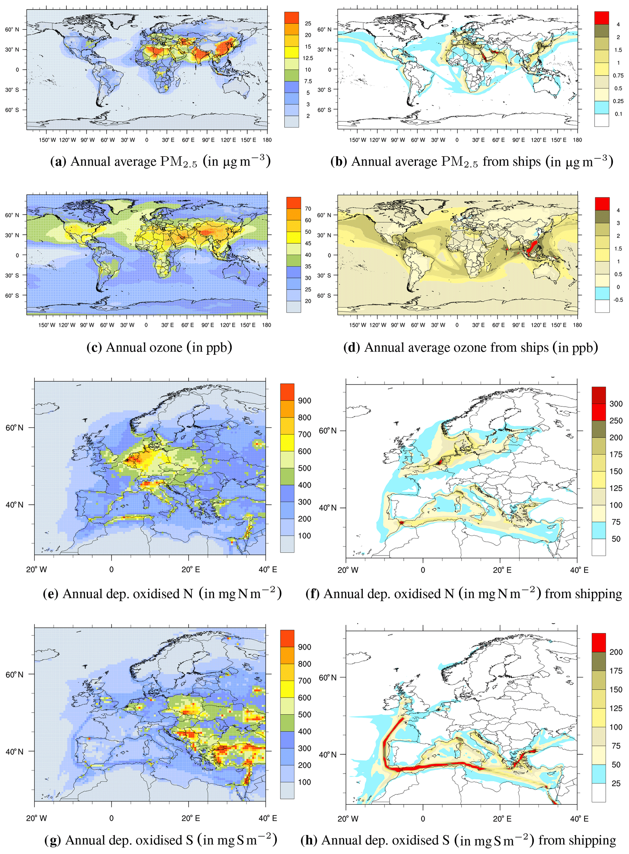
Figure 2 On the right, annually averaged global concentrations of PM_2.5 (a) and O₃ (c). Depositions of oxidised nitrogen (e) and sulfur (g). On the left, contributions from global shipping to PM_2.5 (b) and O₃ (d) and to depositions of oxidised nitrogen (f) and sulfur (h). The contributions from shipping have been multiplied by 100∕15.

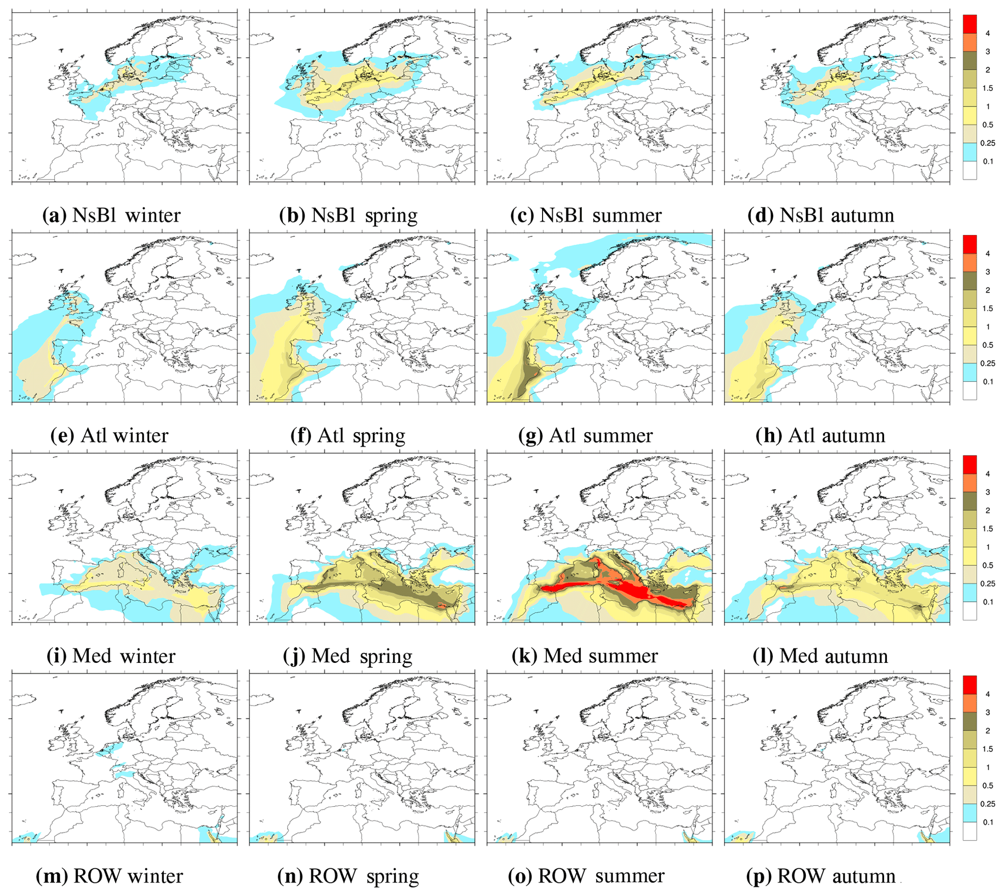
Figure 3 Seasonal contributions to European PM_2.5 levels (in µg m⁻³) from 15 % perturbations of the emissions in separate sea areas defined in Sect. 2.3. Winter is defined as December–January, spring March–May, summer June–August, and autumn September–November. The contributions from shipping have been multiplied by 100∕15.

3.1  PM_2.5

Figure 2 shows the global concentration of PM_2.5 (panel a) and the contributions from global shipping (panel b). Globally, the highest concentrations are calculated over parts of Asia and northern Africa. In Europe, high concentrations are calculated in several locations with the highest concentrations in the Po Valley in Italy. The largest contributions from shipping are mainly calculated in and around the major ship lanes. In Fig. 3, we show to what extent ship emissions from different sea areas contribute to the European PM_2.5 concentrations seasonally. From all sea areas, the largest effects are calculated in nearby countries/regions. Ship emissions generally peak in summer, but the seasonal variations in emissions are not large and far from being large enough to explain the seasonal variations in concentrations seen in Fig. 3. The main sources for particles and particle formation from shipping are NO₂ and sulfur (of which more than 95 % is emitted as SO₂ in the gas phase and the rest as sulfate particles). In addition, ash, EC (elemental carbon), and OC (organic carbon) are assumed to be emitted as primary particles. The main oxidation paths for SO₂ are the OH reaction in the gas phase and in-cloud oxidation (mainly with H₂O₂). Both these oxidants have a clear summer maximum contributing to a summer maximum also for sulfate. In sea areas outside the SECAs, sulfate makes up 50 % to 80 % of the PM_2.5 dry mass (Fig. 8a), explaining the summer maximum in PM_2.5 concentrations in most sea areas.

The second largest fraction is nitrate (Fig. 8b). NO₂ is oxidised to gaseous HNO₃. HNO₃ can then react with sea salt forming particulate sodium nitrate, but these particles are in general large and do not contribute to PM_2.5. However, in the presence of ammonia, the formation of ammonium nitrate particles can be a lot faster. The latter reaction requires a surplus of NH₃ over sulfate. Ammonia is mainly emitted from agriculture with a seasonal maximum in spring. The nitrate fraction from shipping is large in the SECA sea areas where sulfur emissions are very low, and particularly high over land.

Although ammonia is not emitted from ships, nitrate and sulfate from ships increase the formation of ammonium sulfate and ammonium nitrate so that ammonia makes up 20 % to 30 % of the PM_2.5 over parts of the European continent (Fig. 8d). However, as shown in Fig. 3, PM_2.5 concentrations over land are very low except for the coastal zones.

In the SECA sea areas, we calculate that as much as 20 % to 30 % of the PM_2.5 from shipping comes from the primary particles ash, EC, and OC (Fig. 8c).

The effects of the emissions from individual sea areas on PM_2.5 discussed below are based on 2017 ship emissions. The effects of the CAP2020 global reductions in sulfur emissions from ships are described in Sect. 4.

3.1.1 Contributions from the North Sea and the Baltic Sea

For countries/regions bordering the North Sea and the Baltic Sea (Fig. 3a–d), PM_2.5 from local shipping peaks in spring. Following the implementation of the stricter SECA regulations in 2015, sulfur emissions are low (see Table 1). In particular, the south-western parts of this sea area are close to some of the highest ammonia emission regions in Europe. The main source of particles from shipping is NO₂ through the formation of nitrate, predominantly ammonium nitrate. The spring maximum in PM_2.5 from North Sea and Baltic Sea shipping is caused by the interaction with ammonia emissions, mainly from agriculture, peaking in spring.

3.1.2 Contributions from the north-east Atlantic Ocean

The largest contributions to PM_2.5 concentrations in Europe from shipping in the north-east Atlantic (see Fig. 3e–h) are calculated for the regions bordering the ship lane in and out of the Mediterranean through Gibraltar and extending north to the English Channel. As this region is outside the SECA, sulfur emissions are high, and a major constituent in PM_2.5 from shipping is sulfur, emitted mainly as gaseous SO₂ and then oxidised to sulfate. The summer maximum in the contributions from the north-east Atlantic is mainly caused by sulfate.

3.1.3 Contributions from the Mediterranean Sea and the Black Sea

The largest contributions to PM_2.5 concentrations from shipping in the Mediterranean and Black Sea region are calculated in and around the shipping lane from Gibraltar to the Suez Canal. High concentrations are also calculated in and around the Adriatic Sea and around some of the major ports like Marseille in France and Piraeus in Greece. As in the north-east (NE) Atlantic, sulfur emissions from shipping are high, and the summer maximum in this sea area is mainly caused by sulfate.

3.1.4 Contributions from rest of world shipping

Given the large distance to the European continent, contributions to European PM_2.5 levels from ROW shipping are small.

3.1.5 Country attributions

The source receptor relationships for shipping (total and from separate sea areas) are listed in Table 3 for selected countries. Here we also list the corresponding source receptor results as reported in the latest EMEP report (EMEP Status Report 1/2019, 2019). In general, the reported relationships and the results from the global model are in good agreement. Differences between the global and regional calculations are discussed in Sect. 5.

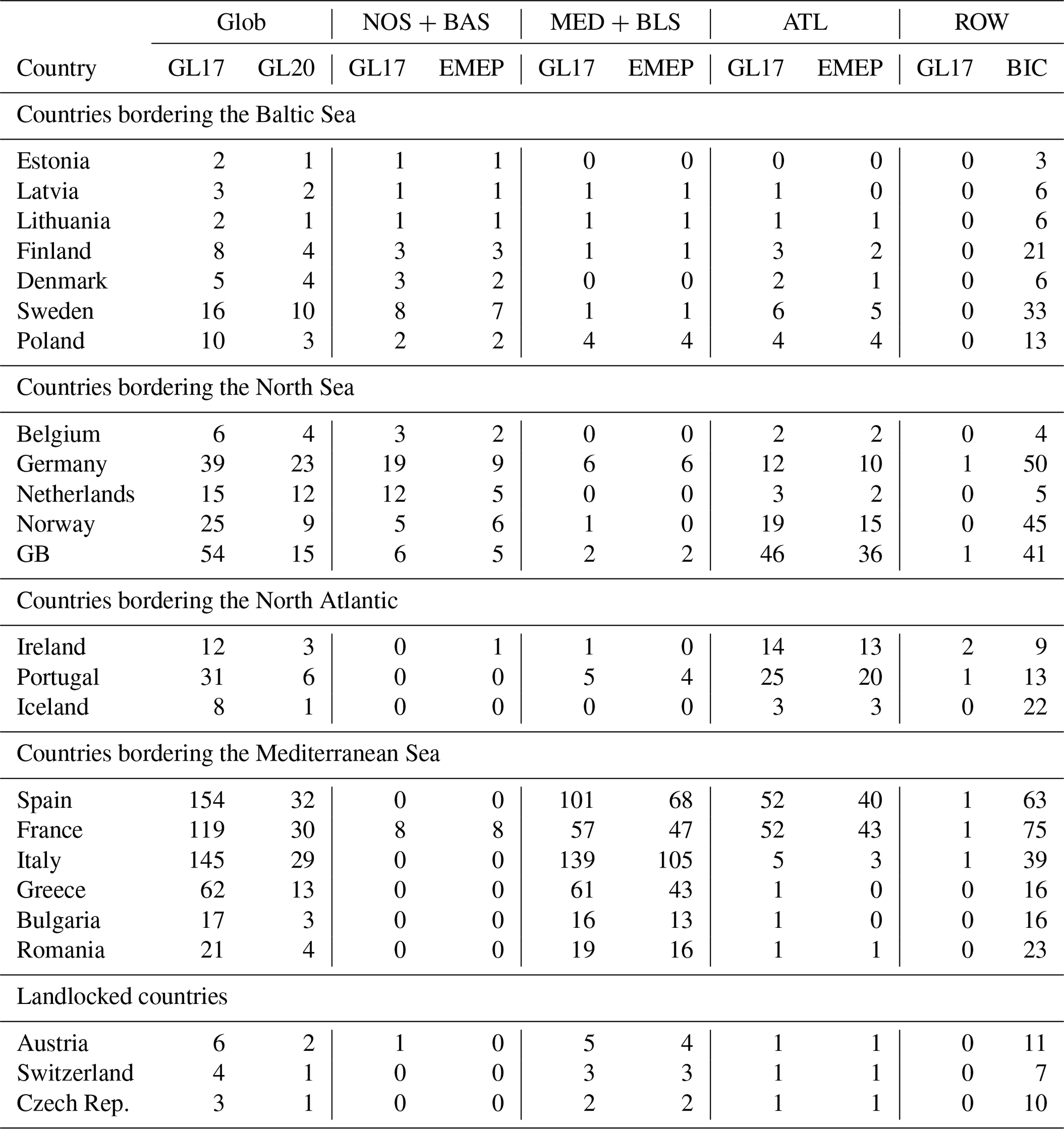
Table 3 Source receptor relationships for PM_2.5 from shipping. GL17 and GL20 are calculated with the global model with 2017 and CAP2020 ship emissions respectively. The scenario calculations are made reducing the ship emissions for all species by 15 %. EMEP is the source receptor calculations for 2017 from the latest EMEP report (Appendix B in EMEP Status Report 1/2019, 2019). The EMEP source receptor report is based on separate calculations of individual species from all European countries and sea areas. Glob is the contribution from all global shipping, NOS + BAS from the North Sea and Baltic Sea combined, MED + BLS from the Mediterranean Sea and Black Sea combined, and ATL from the north-east Atlantic. ROW includes all ship emissions outside the individual sea areas listed. For the EMEP, reported boundary and initial contributions are listed (units: ng m⁻³ per 15 % emission reduction).

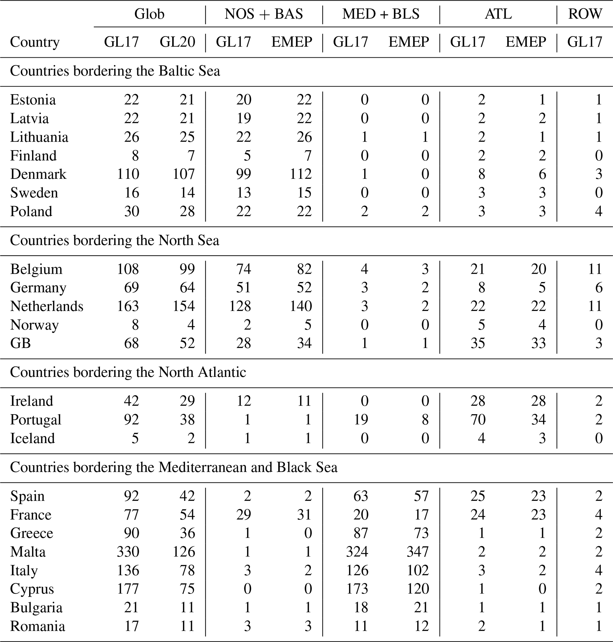
Figure 4 Percentage contributions from shipping to annually averaged PM_2.5 to countries bordering the North Sea and the Baltic Sea (a) and the Mediterranean Sea and the Black Sea (b) relative to contributions from all global anthropogenic emissions. Contributions are shown both for all ships and separated by sea area. For each country, the contributions from the individual sea areas are added in the upper bar and the contributions from all ship emissions calculated as the difference between the Base and SR_AllShips scenarios are shown as black + grey bar below. The Base − SR_AllShips bars are split in a black and grey part in which the first grey part represents the contributions after CAP2020, and black and grey represent the contributions prior to CAP2020. Differences in length between All ships (black and grey) and the added contributions from the separate sea areas are an indication of non-linear effects.

In Fig. 4, the percentage contributions from all ships and from emissions in different sea areas to selected European countries are shown. The contributions are calculated from the scenarios listed in Sect. 2.3. We let the difference between the Base_2017 and the SR_All represent 100 % of the anthropogenic contributions to PM_2.5. The contributions from the individual sea areas are stacked on top of each other. The stacked contributions are shown in parallel to the contributions from all ships (Base_2017–SR_AllSh). Any difference in the length of the two bars can be interpreted as a measure of non-linearities in the calculations. Moderate deviations from linearity are in particular seen for the countries bordering the southern parts of the North Sea and are caused by differences in ammonium nitrate formation between the model scenarios. The contributions from all ships are split into a black and a grey part for which the first grey part represents the contributions with CAP2020 sulfur emissions and the black part the additional contributions when using 2017 emissions, i.e. prior to the implementation of CAP2020. The effects of the CAP2020 regulations are discussed in more detail in Sect. 4.

The figure clearly shows that the countries are most affected by nearby ship emissions, in particular in smaller countries close to major shipping lanes. Malta with about 50 % of the anthropogenic contribution, Cyprus with almost 20 %, and Greece with almost 15 % in the Mediterranean Sea and Denmark, bordering both the North Sea and the Baltic Sea, with about 15 % are some of the countries most affected. Countries bordering only the Mediterranean Sea and the Black Sea are hardly impacted by other sea areas. A few countries are bordering more than one of the separate sea areas. This is exemplified by Norway (about 10 %) and the UK (about 10 %) which are strongly impacted by ship emissions in both the North Sea and the remaining Atlantic. Spain (about 15 %) is impacted by both the remaining Atlantic and the Mediterranean Sea. France (about 8 %) is a “tricolore” country affected by ship emissions in the North Sea, Mediterranean Sea, and remaining Atlantic.

3.2 Ozone

Figure 2c shows the global concentration of O₃ and Fig. 2d the contributions from global shipping. Globally, the highest concentrations are calculated for the latitudinal band between 20 and 40^∘ N. The largest contributions from shipping are mainly calculated in and around the major ship lanes in south Asia, and they result from high NO_x emissions in combination with favourable meteorological conditions for ozone production. In Europe, there are similar favourable conditions in and around the Mediterranean Sea. Below we discuss how ship emissions from different sea areas affect European ozone levels split by season.

Net formation of ozone depends on the ratio between NO_x and NMVOC. In regions with high NO_x concentrations, ozone production is limited by the availability of NMVOC, and further enhancements of NO_x will lead to increased ozone titration and thus reductions in ozone, predominantly in the winter months. In summer, additional NMVOC emissions from leisure boats may lead to an increase in ozone levels in such areas. In areas limited by the availability of NO_x, additional NO_x will result in increased ozone production, predominantly in the summer months.

3.2.1 North Sea and Baltic Sea

In the North Sea and Baltic Sea regions (Fig. 5a–d), ship emissions contribute to widespread ozone titration in all four seasons. The strongest titration effects are calculated in winter and the least in summer.

3.2.2 North-east Atlantic

Although there is a net ozone loss throughout much of the year in the shipping lane from Gibraltar to the entrance of the English Channel, shipping contributes to higher ozone in most of the bordering countries all year with the exception of the UK, northern Scandinavia, and coastal regions next to the shipping lanes. Net ozone production is in particular high in summer (Fig. 5e–h).

Figure 5 Seasonal contributions to European ozone levels (in ppb) from 15 % perturbations of the emissions in separate sea areas defined in Sect. 2.3. Winter is defined as December–January, spring March–May, summer June–August, and autumn September–November. The contributions from shipping have been multiplied by 100∕15.

3.2.3 Mediterranean Sea and Black Sea

In the Mediterranean Sea and the Black Sea, there is widespread ozone titration close to major shipping lanes and ports in winter (Fig. 5i–l). However, in spring, ozone production starts to dominate, reaching a maximum in summer with contributions from shipping of more than 4 ppb (parts per billion) in the eastern Mediterranean Sea and bordering land areas.

3.2.4 Rest of world shipping

Emissions from rest of world shipping affects all of Europe but western and northern Europe more than southern and eastern Europe (Fig. 5m–p). The seasonal behaviour differs from the other sea areas with a summer minimum and a slight winter maximum. On an annual basis, contributions are comparable to, and in some regions higher than, contributions from the other sea areas. This is shown in more detail in the section about country attributions below.

Table 4 Source receptor relationships for SOMO35 from shipping as calculated by the global model, GL17, without ShipNO_x (see Sect. 2) and as reported in Appendix B in EMEP Status Report 1/2019 (2019). All the calculations are made with 2017 emissions and meteorological data. Glob is the contribution from all global shipping, NOS + BAS from the North Sea and Baltic Sea combined, MED + BLS from the Mediterranean Sea and Black Sea combined, and ATL from the north-east Atlantic. ROW includes the effects from all ship emissions outside the above-listed individual sea areas. BIC is regional boundary and initial concentrations (units: ppb⋅day per 15 % emission reduction).

3.2.5 Country attributions

For SOMO35³, the source receptor relationships for shipping (total and from separate sea areas) are listed in Table 4 for selected countries. We also list the corresponding source receptor calculations as reported in the latest EMEP report (EMEP Status Report 1/2019, 2019), and these results are discussed in Sect. 5.

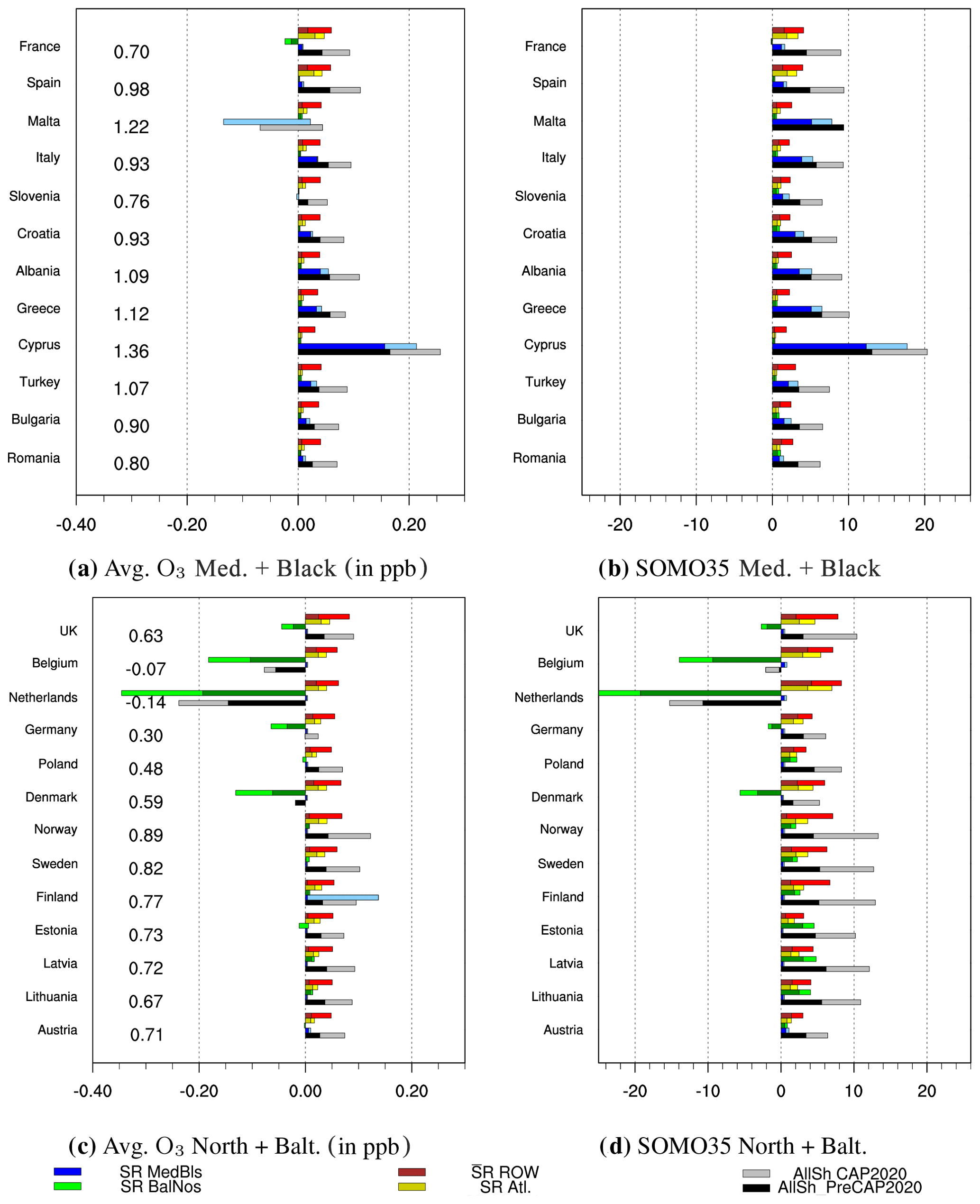
Figure 6 Contributions from shipping (in ppb) to annually averaged ozone from 15 % reductions in ship emissions (a, c). Numbers to the right of the country names are the effects of the 15 % reductions in all anthropogenic emissions calculated as Base_2017–SR_AllSh. (b, d) Percentage contributions to SOMO35 relative to contributions from all global anthropogenic emissions. Contributions are shown for all ships and separated by sea area. The lengths of the bars are split so that the darker parts of the bars represent calculations assuming ShipNO_x (see Sect. 2) and the full length without ShipNO_x. Note that for Malta the smaller perturbation in NO_x from Mediterranean shipping with ShipNO_x results in a small parts per billion increase in calculated ozone, whereas the larger perturbation without ShipNO_x results in a decrease.

In Fig. 6a and c, the contributions from all ship emissions and from emissions in different sea areas to selected European countries are shown for annually averaged ozone (in ppb) following 15 % reductions in ship emissions in the sea areas. The calculated effects of 15 % reductions in all anthropogenic emissions are given as numbers in the figure. In Fig. 6b and d, the effects of ship emissions on SOMO35 are given as a percentage of the total anthropogenic contributionĠiven the non-linear behaviour of the ozone chemistry, contributions from the separate sea areas are not stacked (as for PM_2.5 in Fig. 3). The full length of the bars are split so that the first, darker part of the bars represents the calculations with the ShipNO_x parameterisation included, as described in Sect. 2.3, and the second, brighter coloured part represents the calculations without ShipNO_x. The difference between the calculations with and without ShipNO_x can be interpreted as a range for the effects of ship emissions on ozone levels. In Belgium, the Netherlands, and Malta, the contributions from anthropogenic emissions, and also from ship emissions, to annually averaged ozone are negative as a result of ozone titration.

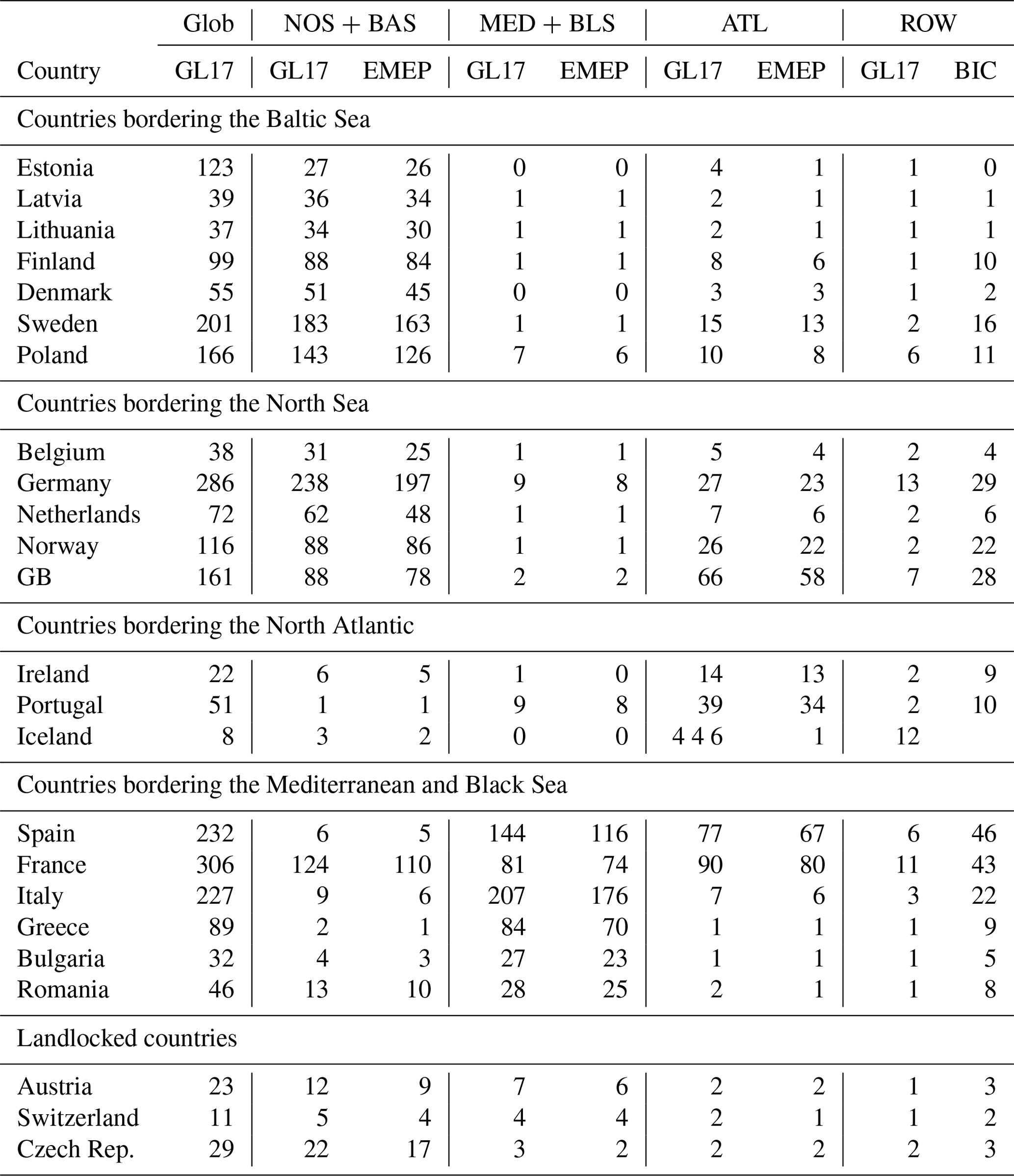
Table 5 Source receptor relationships for depositions of oxidised N “per country” from shipping as calculated by the global model and as reported for the year 2017. Glob is the contribution from all global shipping, NOS + BAS from the North Sea and Baltic Sea combined, MED + BLS from the Mediterranean Sea and Black Sea combined, and ATL from the north-east Atlantic. GL17 is from the global model calculations, and EMEP is from Appendix B in EMEP Status Report 1/2019 (2019) (units: 100 Mg of N per 15 % emission reduction multiplied by 100∕15).

Contrary to what was shown for PM_2.5, there are significant contributions from ROW shipping in most countries, which range from about 5 % to 8 % for countries bordering the North Sea and the Baltic Sea but less for Mediterranean and Black Sea countries. For several countries in western and northern Europe and in landlocked countries exemplified by Austria, as well as in Romania (partially bordering the Black Sea) (Fig. 6), ROW shipping is the largest contributor to anthropogenic ozone levels both with regard to SOMO35 and annual average ozone. In the Mediterranean countries, by far the largest contributions come from Mediterranean shipping with contributions of up to 20 % from Cyprus. In these countries, the second largest contributions are from ROW shipping. In and around the southern part of the North Sea, both land-based and ship emissions of NO_x are high, and, as also shown in Fig. 5a–d, ozone levels decrease as a result of North Sea and Baltic Sea shipping. For the overall effects of shipping, this decrease is compensated for by contributions from other sea areas. However, in Belgium, the Netherlands, and also Malta in the Mediterranean Sea, the overall contributions from ship emissions from all sea areas give reductions in annually averaged ozone levels of the order of 0.1 to 0.2 ppb. In Belgium and the Netherlands, we also calculate reductions in SOMO35 from shipping in the Netherlands by more than 10 % of the contributions from all anthropogenic sources.

3.3 Depositions of sulfur and oxidised nitrogen

Figure 2e and g show the total (wet and dry) depositions of oxidised nitrogen and sulfur centred around Europe. For oxidised nitrogen, large depositions are calculated in north-central Europe and in the Po Valley in Italy. For sulfur, the largest calculated depositions are mainly calculated in eastern Europe.

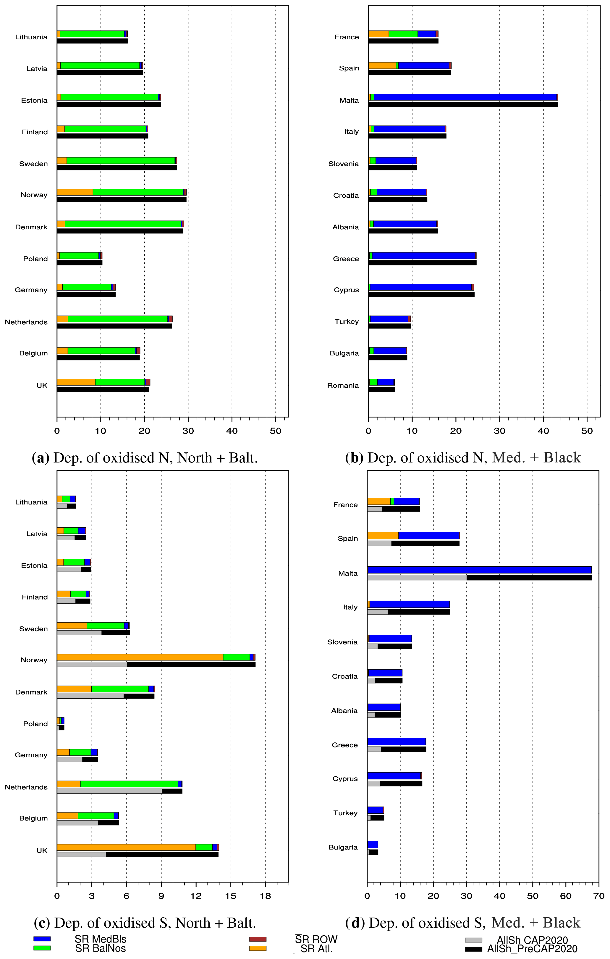
Figure 7 Percentage contributions from shipping to annually averaged depositions of oxidised nitrogen (a, b) and sulfur (c, d) relative to contributions from all global anthropogenic emissions. Contributions are shown for all ships and separated by sea area. See also caption in Fig. 4.

Figure 7 shows the contributions from the separate sea areas to depositions of oxidised nitrogen and sulfur of anthropogenic origin to selected countries. In addition, the source receptor relationships are listed in Tables 5 and 6 for both global and regional model calculations. Depositions from shipping are largely confined to areas/countries near the sea, peaking close to major shipping routes. For most of the coastal countries, the percentage contributions to depositions of oxidised nitrogen are more than 20 %. Even for larger countries like Germany, Poland, France, and Spain, the percentage contributions are 10 % or more. Sulfur depositions from shipping are low in and around the North Sea and Baltic Sea where sulfur emissions are low as a result of the SECA regulations. Even so, contributions from shipping range from 3 % to more than 10 % for these countries. For other coastal countries, contributions range from 10 % to almost 70 % for Malta.

Table 6 Source receptor relationships for depositions of oxidised S from shipping as calculated by the global model and as reported for the year 2017. Glob is the contribution from all global shipping, NOS + BAS from the North Sea and Baltic Sea combined, MED + BLS from the Mediterranean Sea and Black Sea combined, and ATL from the north-east Atlantic. GL17 is from the global model calculations, and EMEP is from Appendix B in EMEP Status Report 1/2019 (2019) (units: 100 Mg of S per 15 % emission reduction multiplied by 100∕15; parts per billion per day per 15 % emission reduction).

4 Effects of CAP2020 on European PM_2.5 levels and on sulfur depositions

From 1 January 2020, the maximum allowed sulfur content in marine fuels was reduced to 0.5 % (CAP2020). Before CAP2020, the global average sulfur content outside SECAs was around 2.5 %, although a higher percentage sulfur content of 3.5 % was allowed. The latest figures showed that the yearly average sulfur content of the residual fuel oils tested in 2017 was 2.54 % (see http://www.imo.org/en/MediaCentre/HotTopics/GHG/Documents/2020 sulphurlimit FAQ 2019.pdf, last access: 7 July 2020). Our calculations show that prior to CAP2020 the fraction of sulfate in PM_2.5 was low in the North Sea and Baltic Sea, as well as in most of continental Europe and the British Isles, as a result of the SECA regulations. However, in sea areas outside the SECA, and in land areas bordering these sea areas, sulfate is the major component in PM_2.5 origination from ship emissions (Fig. 8a).

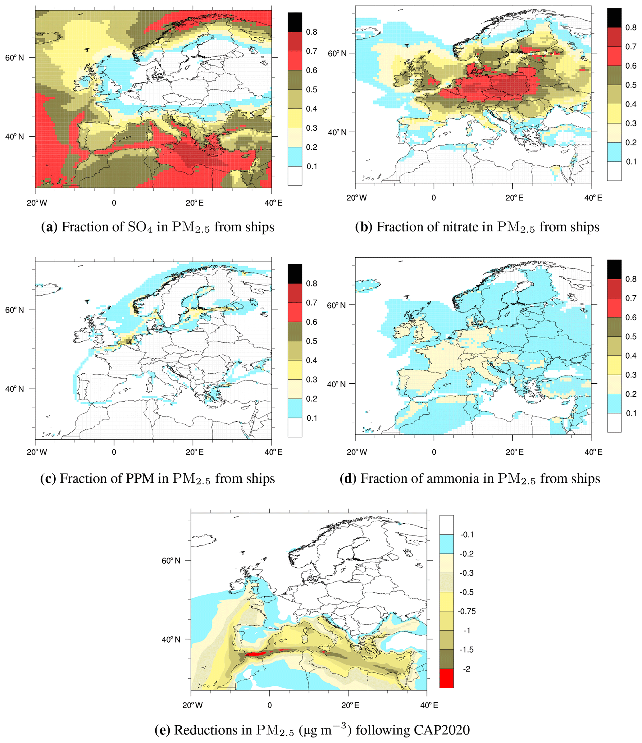
Figure 8 Fraction of (a) SO₄, (b) nitrate, (c) PPM, and (d) ammonia in PM_2.5 in European waters from shipping (a). PPM are ash, EC, and OC. (e) Reductions in PM_2.5 (µg m⁻³) following the CAP2020 regulations.

To give an estimate of the effects of CAP2020 on European PM_2.5 levels and the depositions of oxidised sulfur, we have made calculations reducing sulfur emissions outside the North Sea and the Baltic Sea SECAs by 80 %, corresponding to a reduction from 2.5 % to 0.5 % in the sulfur content in the fuels. This is a crude estimate as there are low-emission ships operating outside the SECAs. On the other hand, CAP2020 compliance may not reach 100 %. Furthermore we have assumed 80 % reductions in sulfur emissions also in low-emission zones far from European waters. But, as already shown in Fig. 3, emissions outside European waters (ROW shipping) have little or no effect on European PM_2.5 levels. Sofiev et al. (2018) estimated a 75 % reduction in global sulfur emissions. As sulfur emissions are already below the CAP2020 levels in the SECAs, this is close to the reduction assumed in this study.

Figure 8b shows the calculated effects of CAP2020 on European PM_2.5 levels. Reductions in PM_2.5 ranging from 0.5 to more than 2 µg m⁻³ are calculated in the major shipping routes in the Mediterranean and eastern Atlantic Ocean, affecting also neighbouring land areas where ship emissions make up a significant percentage of the PM_2.5 concentrations. In Sofiev et al. (2018), they calculate similar reductions ranging from 2 to 4 µg m⁻³ in major shipping lanes, but the largest reductions are calculated for sea areas outside European waters. In European waters north of 62^∘, the sulfur fraction is also high, but here ship traffic is much lower and the effects on PM_2.5 well below 0.1 µg m⁻³.

In Fig. 4, the contributions to PM_2.5 from all ships to selected European countries are shown as a percentage of all anthropogenic contributions calculated from ship emissions before and after the implementation of CAP2020. In particular, in the countries bordering the Mediterranean Sea, the percentage contributions to PM_2.5 relative to all anthropogenic emissions are reduced by about 50 %. For countries bordering the North Sea and the Baltic Sea SECA, where sulfur emissions prior to CAP2020 were very low, the percentage reductions in the contributions to PM_2.5 are much smaller.

A similar pattern as PM_2.5 is seen in Fig. 7 for oxidised sulfur depositions with substantial reductions in depositions of anthropogenic origin in countries bordering sea areas that are not SECAs, such as the Mediterranean Sea and the north-east Atlantic.

5 Differences between regional and global model calculations

The regional model calculations as reported in the annual EMEP reports (exemplified by the latest EMEP report; EMEP Status Report 1/2019, 2019) are widely used for regulative purposes within the EU and for the LRTAP convention (Convention on Long-Range Transboundary Air Pollution; http://www.unece.org/fileadmin//DAM/env/lrtap/welcome.html, last access: 7 July 2020). The alternative global calculations presented here give an indication of the robustness of the officially reported calculations. In general, the results from the global and the regional model calculations are in good agreement. Even so, there are some systematic differences in the model results. We have tried to trace these to differences listed below in model input and model set-up and to what extent global and regional calculations could give qualitatively and quantitatively different results for the effects of ship emissions.

1. As discussed in Sect. 2.2, land-based emissions are not identical.

2. The ship emission sets used in the global and regional calculations have a common origin (see Sect. 2.2). Even so, annual emission totals for the individual sea areas differ. In the global calculations, ship emissions in the individual sea areas are in general higher.

3. In the global model, we reduce the emissions by 15 % for all species in the sea areas simultaneously, whereas in the regional calculations emissions of the individual species are reduced separately.

4. The resolution used in the global and regional model calculations differs.

5. In the regional calculations, the boundary and initial conditions for all gaseous and aerosol species were given as 5-year monthly average concentrations derived from EMEP MSC-W global runs.

Bullet points 3 and 4 were a compromise to keep the computational demand of the global calculations within reasonable limits. Below we discuss the effects this makes for different components in detail. We also make statements on the processes behind these difference, which is of relevance also beyond this study.

5.1 Differences in PM_2.5

For almost all countries bordering the Baltic Sea and North Sea, the effects of ship emissions on PM_2.5 are consistently higher in the global vs. the regional calculations (see Table 3). In most cases, this is because the ship emissions used in the global model are higher than in the regional model calculations (see Sect. 2.2). There are also some additional factors causing differences.

Most countries bordering the Baltic Sea and the North Sea are high emitters of ammonia. SO₄ (either emitted directly or oxidised from SO₂) can react with ammonia forming ammonium sulfate. Much of the emitted NO_x will form HNO₃. Given an excess of ammonia to SO₄, HNO₃ will react with ammonia forming ammonium nitrate. As shown in Table 1, emissions of sulfur in particular in the European Union (and subsequently in countries bordering these two sea areas) are higher in the global model calculations. In addition, sulfur emissions are slightly higher in the remaining north-east Atlantic. As a result, more sulfate is available for ammonium sulfate formation, thereby allowing less of the HNO₃ from shipping to form particulate ammonium nitrate. This explains the lower formation of PM_2.5 from shipping in the vicinity of regions of high ammonia emissions.

In several countries, PM_2.5 levels from shipping are markedly higher in the global calculation, in particular in small countries such as Cyprus and also in Portugal where the shipping lanes are very close to the shore. We believe this is caused by the lower resolution in the global calculations, which implies that grid boxes partially covering land and sea extend further inland, thus artificially extending the effect of ship emissions somewhat further into these countries' territories.

5.2 Differences in nitrogen and sulfur deposition between global and regional model calculations

Depositions of both oxidised nitrogen and sulfur are in general higher in the global model calculations as a result of higher emissions used in the global model. Above we argued that parts of the lower contributions from ships to PM_2.5 concentrations could be caused by less ammonia available for ammonium nitrate formation in the global calculations, resulting in a higher HNO₃ to ammonium nitrate ratio. As the dry deposition of HNO₃ is faster than for ammonium nitrate, more oxidised nitrogen (mainly ammonium nitrate, HNO₃, NO₂) is deposited in nearby countries where ammonia emissions are high.

In several countries, both nitrogen and sulfur depositions are higher in the global model calculations than what can be explained by differences in emissions alone, in particular in small countries such as Malta and Cyprus and in Portugal where the shipping lanes are very close to the shore. As for PM_2.5 concentrations, we believe this is caused by a lower resolution in the global calculations as grid boxes partially covering land and sea extend further inland.

5.3 Differences in SOMO35

In Table 4, the contributions from ship emissions to selected countries are listed for both the global and regional model calculations. Note that there are large, compensating budget terms involved in how ship emissions effect surface ozone concentrations, namely substantial ozone production, especially in summer, and ozone titration mainly outside the summer months. Despite considerable uncertainties in these terms, the SOMO35 values calculated with the global and the regional model versions are remarkably similar. However, there are substantial differences mainly confined to the very high NO_x emitting regions bordering the North Sea.

In the global calculations, there are substantial contributions from ROW shipping (see Table 4) that can not be attributed in the regional calculations, and in several countries ROW is the largest contributor (see Sect. 3.2.5).

With the ShipNO_x parameterisation included in the global calculations, the contributions to SOMO35 from the sea areas are reduced by about 50 % (see Fig. 6) and considerably lower than in the regional calculations. ShipNO_x is not used in the regional calculations, but the largest effects of ignoring the ship plume chemistry should be in low NO_x areas with large gradients between the plumes and ambient air most often found in pristine sea areas.

6 Conclusions

Emissions from shipping are large sources of air pollution and depositions of oxidised nitrogen and sulfur. In this study, we have mainly restricted ourselves to the effects on European pollution levels, but the effects are global. In particular, in coastal regions/countries, we attribute a large portion of the PM_2.5 of anthropogenic origin to emissions from shipping. For PM_2.5, we show that the largest contributions come from nearby waters. The calculations show that contributions from sulfur to PM_2.5 are low from the North Sea and the Baltic sea where the strict SECA regulations apply. Prior to the implementation of the CAP2020 regulations, between 50 % and 80 % of the anthropogenic PM_2.5 mass in countries/regions not bordering the SECAs was from sulfate. Here sulfate levels peak in summer when the conversion rate of SO₂ to sulfate is at its highest. In the SECA sea areas, nitrates (mainly ammonium nitrate) are the largest constituent in anthropogenic PM_2.5, peaking in spring as a result of the large ammonia emissions in nearby land areas in this season. With additional sulfate and gas phase HNO₃ from ship emissions, more ammonia (ammonium nitrate and ammonium sulfate) is formed, contributing about 20 %–30 % of the PM_2.5 dry mass from shipping in much of the European land area. As a result, the combination of sulfur and NO_x emissions from shipping further increases the PM_2.5 burden in and around regions with high ammonia emissions beyond what strictly speaking is originating directly from SO_x and NO_x. Without ship emissions, a larger portion of the ammonia would have been deposited at the surface and would not have contributed to the particle formation.

The very low fraction of sulfate in PM_2.5 in and around the North Sea and the Baltic Sea demonstrates the effectiveness of the SECA regulations in reducing the PM_2.5 burden from shipping here. A global sulfur cap was implemented on 1 January 2020. Assuming the fulfilment of the legislation, it is expected that this has now resulted in substantial reductions in the PM_2.5 burden globally. This has resulted in approximately 50 % reductions in calculated PM_2.5 from shipping in European countries and regions not bordering the SECAs. In a similar study, using the SILAM model, Sofiev et al. (2018) calculated reductions in PM_2.5 levels in the busiest sea lanes of 2 to 4 µg m⁻³. This is similar to the total contribution from shipping shown in Fig. 2 (100 % vs. 80 % sulfur control).

In Karl et al. (2019), the SILAM model, along with the CMAQ model, was compared to the EMEP model focusing on the effects of ship emissions in the Baltic Sea in 2012 prior to the implementation of stricter SECA regulations in 2015. As noted in Sect. 2.1, the CMAQ and the EMEP models had a slightly negative bias for PM_2.5, whereas the SILAM model had virtually no bias. Even so, the SILAM model calculated a slightly lower contribution from Baltic Sea shipping compared to the other two models. In this study, using year 2012 emissions, the average contribution from ships to PM_2.5 levels ranged between 4.15 % and 6.5 % in the entire Baltic Sea region and between 3.15 % and 5.7 % in the coastal land areas. For the year 2017, these contributions were considerably lower, as was also shown in Jonson et al. (2019).

In Chinese coastal regions, the peak contributions to PM_2.5 concentrations in this study are lower than in the study by Lv et al. (2018). There are several possible explanations for this difference. Lv et al. (2018) used a finer model resolution (36 km×36 km) than in the present study. A finer resolution is likely to result in somewhat higher peak concentrations. Stricter regulations limiting the sulfur content in marine fuels to 0.5 % in and around several Chinese ports, including the YRD (Yangtze River Delta), have been imposed between these two studies (2013 vs. 2017) and are included in the ECCAD 2017 ship emission data. According to Lv et al. (2018), the YRD is responsible for about 20 % of the ship emissions in Chinese waters.

The net effects on surface ozone from ship emissions is a combination of ozone destruction, mainly in winter, and ozone production, mainly in summer. This is also the reason for the different behaviour of annual averaged ozone and the SOMO35 ozone metric. SOMO35 is hardly accumulated in winter when ozone titration events are most frequent as ozone levels in winter are regularly below the 35 ppb threshold.

The lifetime of ozone in the atmosphere is considerably longer than for PM_2.5, ranging from hours to a few days in the boundary layer to weeks and even months in the free troposphere (TF HTAP, 2010). As a result, ozone can be transported at intercontinental scales, which explains the large contributions from ROW shipping.

Global model calculations require substantially more computer power than regional calculations, and thus global-scale source receptor calculations, even with a half a degree resolution, would not be possible with all countries and regions included in the regional-scale calculations. The source receptor relationships derived from the global and regional calculations are similar. Where there are differences, these can largely be attributed to model set-up and input data. Most of the species levels, and the resulting surface depositions, highlighted in EMEP regional calculations are relatively short-lived. As a result, the effects of emissions originating outside the regional model domain are small. Thus, the additional benefits of global model calculations are small compared to the improvements in accuracy that can be achieved with finer resolutions on a smaller model domain. For ozone, enhancing the resolution improves the representation of localised variations in NO_x to NMVOC ratios, which explains in particular the differences in the high NO_x emitting countries and regions bordering the North Sea. On the other hand, with global-scale calculations, the contributions to ozone from all global sources can be included. For several countries/regions, we show that, for ozone, contributions from ROW shipping are comparable, and in some regions higher than the contributions from sea areas close to Europe. In the regional model source receptor calculations, BICs (boundary and initial concentrations) only account for ozone produced within the regional model domain from NO_x (emissions of NMVOC from shipping are very small) transported from outside the regional model domain.

The dispersion and chemistry in the shipping plumes represent an uncertainty in the calculations. Calculations including the ShipNO_x parameterisation short-circuit the NO_x chemistry so that only half of the emitted NO_x enters the ozone cycle, and as a result the effect of shipping on ozone is also reduced by about 50 %. Calculations with and without the ShipNO_x parameterisation give an upper and lower range for the effects of shipping on ozone. The largest effects of ship plume chemistry are likely to occur where the gradients between ship plume and ambient air NO_x concentrations are large. Such conditions are less common in waters close to Europe. In their plume calculations, Vinken et al. (2011) reported that almost all the ozone was depleted in the first stages of the plume. In Karl et al. (2019), the EMEP model, with its coarser grid resolution, calculated less ozone titration in the shipping lanes. However, downwind of the shipping plumes, ozone is regenerated. As a result, the impact of ship emissions on ozone in nearby land areas was comparable for the EMEP and CMAQ models but lower for the SILAM model. These results partially corroborate the chemistry in plumes outlined by Vinken et al. (2011) but also demonstrate the regeneration of ozone downwind of the ship plumes.