the Creative Commons Attribution 4.0 License.
the Creative Commons Attribution 4.0 License.
 | 01 Oct 2020
Trends of atmospheric water vapour in Switzerland from ground-based radiometry, FTIR and GNSS data
Elmar Brockmann
Thomas von Clarmann
Niklaus Kämpfer
Emmanuel Mahieu
Christian Mätzler
Gunter Stober
Klemens Hocke
Vertically integrated water vapour (IWV) is expected to increase globally in a warming climate. To determine whether IWV increases as expected on a regional scale, we present IWV trends in Switzerland from ground-based remote sensing techniques and reanalysis models, considering data for the time period 1995 to 2018. We estimate IWV trends from a ground-based microwave radiometer in Bern, from a Fourier transform infrared (FTIR) spectrometer at Jungfraujoch, from reanalysis data (ERA5 and MERRA-2) and from Swiss ground-based Global Navigation Satellite System (GNSS) stations. Using a straightforward trend method, we account for jumps in the GNSS data, which are highly sensitive to instrumental changes. We found that IWV generally increased by 2 % per decade to 5 % per decade, with deviating trends at some GNSS stations. Trends were significantly positive at 17 % of all GNSS stations, which often lie at higher altitudes (between 850 and 1650 m above sea level). Our results further show that IWV in Bern scales to air temperature as expected (except in winter), but the IWV–temperature relation based on reanalysis data in the whole of Switzerland is not clear everywhere. In addition to our positive IWV trends, we found that the radiometer in Bern agrees within 5 % with GNSS and reanalyses. At the Jungfraujoch high-altitude station, we found a mean difference of 0.26 mm (15 %) between the FTIR and coincident GNSS data, improving to 4 % after an antenna update in 2016. In general, we showed that ground-based GNSS data are highly valuable for climate monitoring, given that the data have been homogeneously reprocessed and that instrumental changes are accounted for. We found a response of IWV to rising temperature in Switzerland, which is relevant for projected changes in local cloud and precipitation processes.
- Article
(7128 KB) - Full-text XML
- BibTeX
- EndNote


Atmospheric water vapour is a key component in the climate system. It is the most abundant greenhouse gas and is responsible for a strong positive feedback that enhances temperature increase induced by other greenhouse gases (e.g. IPCC, 2013; Stocker et al., 2001). Furthermore, water vapour is involved in important tropospheric processes such as cloud formation and precipitation; it influences size, composition and optical properties of aerosols; and it is responsible for atmospheric energy and heat transport via evaporation and condensation (Kämpfer, 2013). Measuring changes in atmospheric water vapour is thus important because they reflect externally forced temperature changes in the climate system and can be an indicator for changes in involved processes such as cloud formation and precipitation. Concentrating here on regional changes is of special interest because water vapour is spatially variable and the relation between water vapour, temperature and precipitation shows spatial dependencies.
Temperature and water vapour are closely linked as expected from the Clausius–Clapeyron relation. Several studies have revealed spatial correlation between mass changes in vertically integrated water vapour (IWV) and changes in temperature, especially over oceans (e.g. Wentz and Schabel, 2000; Trenberth et al., 2005; Wang et al., 2016). Nevertheless, it has also been shown that water vapour does not scale to temperature everywhere as expected and that large regional differences exist (e.g. O'Gorman and Muller, 2010; Chen and Liu, 2016; Wang et al., 2016). Over continental areas, correlations between surface temperature and IWV changes are smaller than over oceans, even showing opposite trends in some regions (Wagner et al., 2006). Also, temperature climate feedbacks may have regional dependencies (Armour et al., 2013). Regional analyses of changes in water vapour and the relation to temperature changes are thus required.
Most of the atmospheric water vapour resides in the troposphere. Measuring IWV, vertically integrated over the whole atmospheric column, is therefore representative of tropospheric water vapour. The IWV can be measured by different techniques. Nadir sounding satellite techniques provide global data sets of IWV that have been used for global trend analyses in multiple studies (e.g. Trenberth et al., 2005; Santer et al., 2007; Wentz et al., 2007; Mieruch et al., 2008; Hartmann et al., 2013; Ho et al., 2018; Zhang et al., 2018). Most of these studies found global IWV trends between 1 % per decade and 2 % per decade, with large spatial differences. However, these satellite data sets have some limitations for regional IWV trend analyses. First, missing homogenization across multiple satellite platforms can make satellite trend studies difficult (Hartmann et al., 2013; John et al., 2011). Second, visible and infrared satellite techniques are limited to clear-sky measurements. Furthermore, satellite products from passive microwave sensors are restricted to oceans only, because the well-known ocean surface emissivity makes retrievals generally easier over oceans than over land surfaces (Urban, 2013). Stable and long-term station measurements from ground are therefore more appropriate for regional IWV trend analyses over land. From ground, IWV can be measured by radiosondes (Ross and Elliot, 2001), sun photometers (precision filter radiometers, PFRs, Ingold et al., 2000; Wehrli, 2000), Fourier transform infrared (FTIR) spectrometers (Sussmann et al., 2009; Schneider et al., 2012) or microwave radiometers (Morland et al., 2009). Radiosondes provide the longest time series, but the homogeneity of the records can be problematic due to changes in instrumentation or observational routines (Ross and Elliot, 2001), and the temporal sampling is sparse (usually twice a day). PFR and FTIR instruments measure during day and clear-sky conditions only, whereas microwave radiometers can measure in almost all weather conditions during day and night with high temporal resolution. However, no dense measurement network exists for these techniques. Another technique that provides data in all weather situations is the use of ground-based receivers of the Global Navigation Satellite System (GNSS). The advantage of GNSS receivers is the high spatial resolution due to dense networks. In the present study we combine the microwave and FTIR techniques at two Swiss measurement stations with data from the ground-based GNSS network in Switzerland to analyse IWV trends.
Several studies use GNSS measurements to derive global IWV trends over land (e.g. Chen and Liu, 2016; Wang et al., 2016; Parracho et al., 2018). Chen and Liu (2016) report GNSS-derived IWV trends at mid-latitudes of 1.46 % per decade, and Parracho et al. (2018) found IWV trends in the Northern Hemisphere of approximately 2.6 % per decade based on GNSS and reanalysis data. The high spatial resolution of some regional GNSS networks makes them a valuable data set for regional trend analyses of IWV. For Europe, IWV trends based on GNSS data have been presented, for example, for Germany (Alshawaf et al., 2017) and Scandinavia (Nilsson and Elgered, 2008), reporting a large trend variability between different stations.
To the best of our knowledge, no regional analysis of IWV trends covering the whole area of Switzerland has been published so far. Some studies presented IWV trends at single Swiss stations (Morland et al., 2009; Sussmann et al., 2009; Hocke et al., 2011, 2016; Nyeki et al., 2019), but most of them cover shorter time periods than available today. Morland et al. (2009) and Hocke et al. (2011, 2016) presented IWV trends at Bern using the same microwave radiometer that we use in the present study. However, they use time series of a maximum of 13 years, whereas a time series of 24 years (1995–2018) is available now. Given that Switzerland experienced strong warming in the last decade, an update is of particular interest. Indeed, 9 of the warmest 10 years in Switzerland (from 1864 to 2018) have occurred in the last two decades, and 6 of the years lie in the last decade (NCCS, 2018). A recent study by Nyeki et al. (2019) presents GNSS-based trends for longer time series (until 2015), but they concentrate only on four Swiss stations. In fact, none of the mentioned studies presents IWV trends in the whole of Switzerland.
Our study presents a complete trend analysis of IWV in Switzerland based on data from the Swiss GNSS station network, a microwave radiometer located in Bern, an FTIR spectrometer located at Jungfraujoch and from reanalysis models. We present IWV trends for time series of 24 years (radiometer, FTIR and reanalyses) or 19 years (GNSS) and analyse how they are related to observed changes in temperature. To avoid artificial trends, homogenized radiometer data have been used in the present study (Morland et al., 2009; Hocke et al., 2011). For the GNSS data, possible jumps due to instrumental changes have been considered in the trend analysis by using the feature of bias fitting in the trend programme of von Clarmann et al. (2010). The goal of our study is to present trends of IWV in Switzerland, to detect potential regional differences and to verify if water vapour increases as expected from the observed temperature rise.
We compare IWV data from a microwave radiometer located in Bern and an FTIR spectrometer at Jungfraujoch with Swiss GNSS ground stations and reanalysis data (ERA5 and MERRA-2). Radiometer data are available from 1995 onwards. We therefore define our study period from January 1995 to December 2018, even though GNSS data are available only after 2000 (see Table 1). IWV is often given as the total mass of water vapour per square metre (kg m−2). However, we provide IWV data in millimetres, taking the density of water into account, which is often referred to as “total precipitable water vapour”. Evidently not all of the water vapour is actually precipitable. To avoid confusion, we prefer the term integrated water vapour (IWV) and provide the amount in the more convenient unit of millimetres, where 1 mm corresponds to 1 kg m−2.
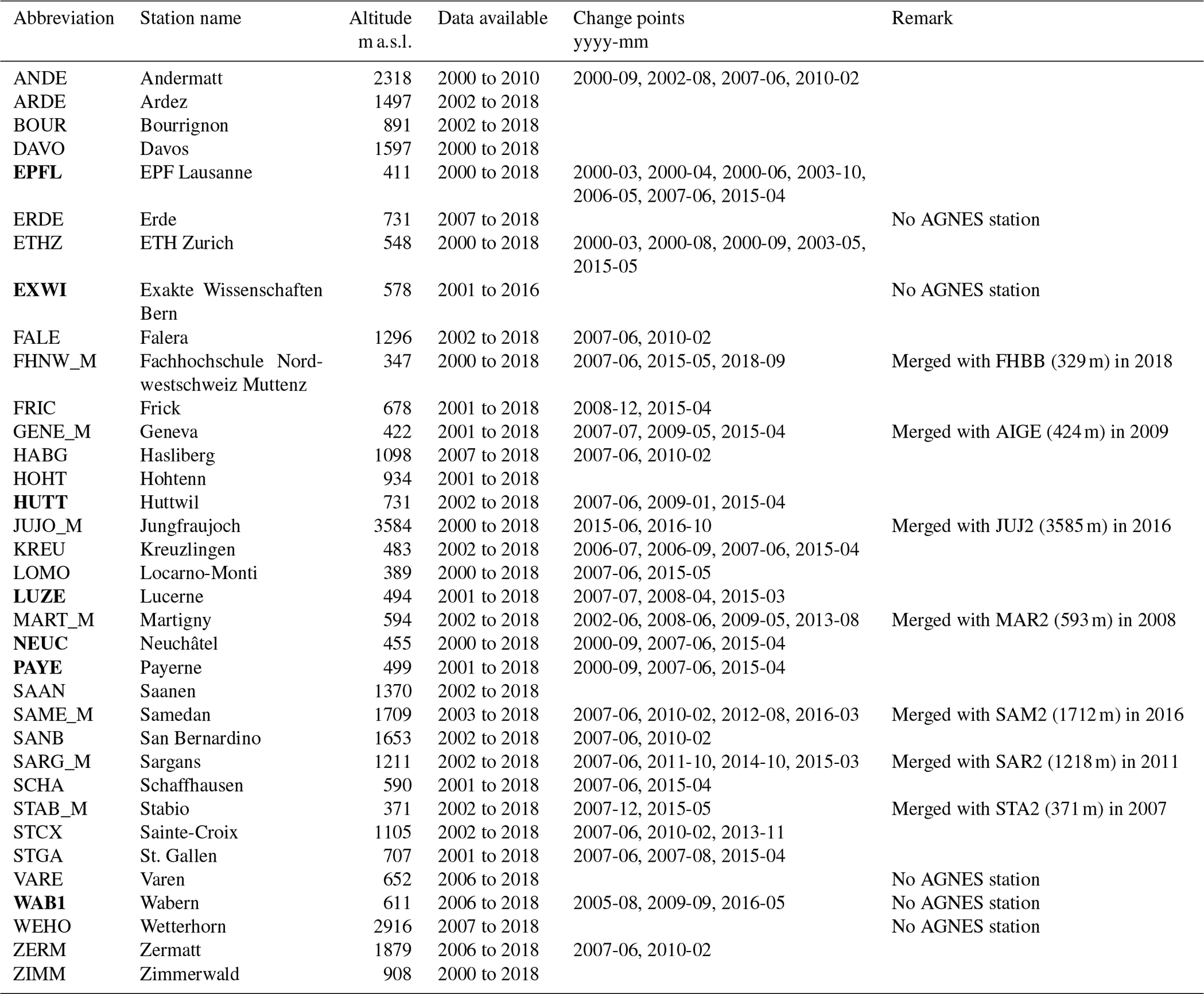
Table 1Swiss GNSS stations used in the present study. Stations marked in bold were directly compared with radiometer and reanalysis data at Bern (latitude = 46.95±0.5∘, longitude = 7.44±1∘, altitude = 575±200 m).
2.1 Microwave radiometer
The Tropospheric Water Vapour Radiometer (TROWARA) is a microwave radiometer that has been retrieving IWV and integrated liquid water (ILW) since November 1994 in Bern, Switzerland (46.95∘ N, 7.44∘ E; 575 m above sea level, a.s.l.). It measures the thermal microwave emission at the frequencies of 21.39, 22.24 and 31.5 GHz with a time resolution of several seconds and an elevation angle of 40∘. The measured signal is used to infer the atmospheric opacity, using the Rayleigh–Jeans approximation of the radiative transfer equation as described in Mätzler and Morland (2009) and Ingold et al. (1998).
The opacity linearly depends on the water content in the atmosphere and can therefore be used to derive IWV and ILW (Mätzler and Morland, 2009; Hocke et al., 2017):
where τi is the opacity of the ith frequency channel of the radiometer. The coefficients ai and bi are statistically derived from nearby radiosonde measurements and fine-tuned with clear-sky measurements (Mätzler and Morland, 2009). The coefficient ci is the Rayleigh mass absorption coefficient of liquid water.
The initial instrument setup and measurement principle is presented in Peter and Kämpfer (1992). To improve the measurement stability and data availability, the instrument was upgraded in 2002 and 2004 and a new radiometer model was developed (Morland, 2002; Morland et al., 2006). Furthermore, it was moved into an indoor laboratory in November 2002, which made it possible to measure IWV even during light-rain conditions (Morland, 2002). However, to maintain consistency with the measurements before 2002, data observed during rainy conditions were excluded in the present study as soon as the ILW exceeded 0.5 mm or rain was detected by the collocated weather station (Morland et al., 2009). We use hourly IWV data from the STARTWAVE database (http://www.iapmw.unibe.ch/research/projects/STARTWAVE/, last access: 29 September 2020) which were derived from the opacities at 21.39 and 31.5 GHz. Before 2008, we use TROWARA data in which data gaps were filled with data derived from a collocated radiometer as described by Hocke et al. (2011) and Gerber (2009). Furthermore, change points in TROWARA data due to instrumental changes have been detected and corrected by a careful comparison of the TROWARA time series before 2008 with simultaneous measurements from other techniques (Morland et al., 2009). No instrumental changes have been performed in recent years. We therefore presume that the data are well homogenized and suitable for trend estimation.
2.2 Fourier transform infrared spectrometer
A ground-based solar Fourier transform infrared (FTIR) spectrometer is located at the high-altitude observatory Jungfraujoch in Switzerland (46.55∘ N, 7.98∘ E; 3580 m a.s.l.). Water vapour information is retrieved from absorption in the solar spectrum at three spectral intervals within 11.7 and 11.9 µm. The optimized IWV retrieval for FTIR spectrometry is described by Sussmann et al. (2009), and instrumental details are given in Zander et al. (2008). FTIR measurements at Jungfraujoch provide water vapour data since 1984. For consistency with our study period, we use data only from 1995 to 2018. In this period, two FTIR instruments were installed at Jungfraujoch, with overlapping measurements from 1995 to 2001. Sussmann et al. showed that the bias between both instruments is negligible. We therefore compute monthly means of a merged time series including both instruments. FTIR measurements are weather dependent (cloud-free conditions are required) and thus provide irregularly sampled data at Jungfraujoch, with on average eight measurement days per month in our study period. This sparse sampling can be problematic when calculating monthly means. We therefore apply the resampling method proposed by Wilhelm et al. (2019) when calculating monthly means of FTIR-derived IWV. For this, the background IWV data are determined by fitting a seasonal model to daily IWV means. The seasonal model is given by a mean IWV0, the first two seasonal harmonics with periods , and the fit coefficients an and bn:
This seasonal model is fitted to the 15th of each month using a window length of 2 years. Due to the sparsity of the FTIR data, the model fit to each month provides a more robust estimate compared to the statistical monthly means, which might be based on only 1 or 2 d of observations at the beginning or end of a month that are not necessarily representative as a monthly mean. The measurement uncertainties of the obtained monthly mean values are derived from the covariance matrix of the model fit. Furthermore, we also tested a seasonal model with higher seasonal harmonics. However, due to the sparse FTIR measurements it appeared not to be useful to improve the obtained monthly mean IWV estimates.
2.3 GNSS ground stations
The signal of GNSS satellites is delayed when passing through the atmosphere. This so-called zenith total delay (ZTD) can be used to infer information about the atmospheric water vapour content. Various studies explain the method to derive IWV from the measured ZTD (e.g. Bevis et al., 1992; Hagemann et al., 2002; Guerova et al., 2003; Heise et al., 2009). We briefly summarize the procedure that we used in our study. The ZTD can be written as the sum of (i) the zenith hydrostatic delay (ZHD) due to refraction by the dry atmosphere and (ii) the zenith wet delay (ZWD) due to refraction by water vapour (Davis et al., 1985):
The ZHD (in metres) is calculated from the surface pressure at each GNSS station as proposed by Elgered et al. (1991):
with surface pressure ps in hectopascals. The dependency of the gravitational acceleration on latitude and altitude is considered in the function f (Saastamoinen, 1972):
where λ is the station latitude in degrees and H is the station altitude in kilometres. With the measured ZTD and the calculated ZHD, we obtain the ZWD (Eq. 3), which can then be used to infer information about the IWV in millimetres. It is calculated according to Bevis et al. (1992) with
where is the density of liquid water ( kg m−3). The factor κ is given by
with the constants k3 and as derived by Davis et al. (1985) from Thayer (1974) ( K2 hPa−1 and K hPa−1). The required estimate of the mean atmospheric temperature Tm is linearly approximated from the surface temperature Ts (damped with the daily mean) as proposed by Bevis et al. (1992) (). Another possibility would be to estimate Tm from reanalysis data. However, GNSS estimates would then depend on reanalyses, which would make validation of GNSS with reanalyses problematic. Furthermore, Alshawaf et al. (2017) showed that the use of reanalyses temperature and pressure data can lead to a bias in IWV compared to the use of surface measurements, especially in mountainous regions in Germany. We therefore follow their recommendation to use the Bevis approximation derived from surface temperature. The pressure ps and the surface temperature Ts at the GNSS station are vertically interpolated from pressure and temperature measurements at the closest meteorological station, assuming hydrostatic equilibrium and an adiabatic lapse rate of 6.5 K km−1.
We use hourly ZTD data from the Automated GNSS Network for Switzerland (AGNES), containing 41 antennas (at 31 locations), as well as data from a few stations that are part of the COGEAR network (https://mpg.igp.ethz.ch/research/geomonitoring/cogear-gnss-monitoring.html, last access: 29 September 2020) and from two additional stations in Bern. The AGNES network was established in 2001 (Schneider et al., 2000; Brockmann, 2001; Brockmann et al., 2001a, b), and it is maintained by the Swiss Federal Office of Topography (swisstopo). A monitor web page shows the current status of all stations (Swisstopo, 2019). In 2008, most of the antennas and receivers were enhanced from GPS only to GPS and GLONASS (Russian global navigation satellite system). Since spring 2015, AGNES has been a multi-GNSS network (Brockmann et al., 2016) also using data from Galileo (European global navigation satellite system) and BeiDou (Chinese navigation satellite system). All European GNSS data were reprocessed in 2014 within the second EUREF (International Association of Geodesy Reference Frame Sub-Commission for Europe) Permanent Network (EPN) reprocessing campaign as described in Pacione et al. (2017). In the present study, only the reprocessed ZTD products of swisstopo are used (Brockmann, 2015).
The stations used in our study are shown in Fig. 1 and listed in Table 1. We only use stations that provide measurements for more than 10 years. At some GNSS stations, a new antenna and receiver were installed at the same or nearby location, replacing the older ones after an overlapping measurement period. An antenna change often leads to a small height difference, which can lead to a jump in the ZTD time series. It is therefore important to decide how to handle such instrumental changes for trend analyses. In cases of antenna and receiver replacements, we merged these stations to a single time series by calculating the mean value for overlapping periods. They are marked by “_M” (for “merged”) in their station abbreviation (Table 1), and a potential jump was considered in the trend estimation (see Sect. 3.1). At nine stations, new multi-GNSS receivers and antennas were installed at an additional location nearby, but the old GPS-only receivers and antennas are still operating. Swisstopo installed such twin stations to ensure a best possible long-term consistency. Simply replacing antennas at all stations would not guarantee continuous time series, even if the phase centres of the antennas were individually calibrated. Furthermore, no calibrations have been available for the tracked satellite systems Galileo and BeiDou until today. In the case of twin stations, we only used the old, continuous GPS-only station, because the stability is better suited for trend calculations than merged time series with potential data jumps.
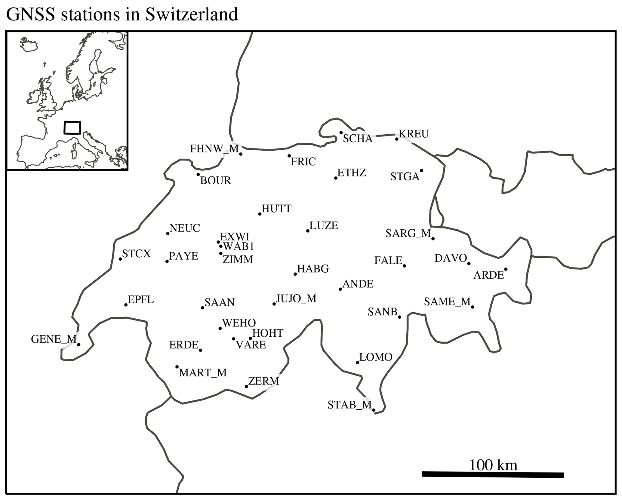
Figure 1Map of Swiss Global Navigation Satellite System (GNSS) stations used in this study.
2.4 Reanalysis data
IWV, relative humidity (RH) and temperature data from two reanalysis products are used in the present study, the ERA5 and the MERRA-2 reanalyses. The Modern-Era Retrospective Analysis for Research and Applications, version 2 (MERRA-2), is an atmospheric reanalysis from NASA's Global Modeling and Assimilation Office (GMAO), described in Gelaro et al. (2017). The MERRA-2 product used in the present study for IWV data contains monthly means of vertically integrated values of water vapour (Global Modeling and Assimilation Office (GMAO), 2015) with a grid resolution of 0.5∘ latitude × 0.625∘ longitude. The ERA5 reanalysis is the latest atmospheric reanalysis from the European Centre for Medium Range Weather Forecasts (ECMWF) (Hersbach et al., 2018). In the present study, we use an ERA5 product providing integrated water vapour (Copernicus CDS, 2019a) and another product providing RH and temperature profiles (Copernicus CDS, 2019b), both with a grid resolution of 0.25∘ latitude × 0.25∘ longitude (Copernicus Climate Change Service (C3S), 2017). Reanalysis models assume a smooth topography that can deviate from the real topography, especially in mountainous regions (Bock et al., 2005; Bock and Parracho, 2019). For validation of reanalysis data with specific station data (e.g. GNSS), the reanalysis IWV value would need to be corrected for altitude differences as proposed by for example Bock et al. (2005) or Parracho et al. (2018). For linear trends, however, such a linear correction is not relevant. We therefore use uncorrected reanalysis data, which might lead to some differences in IWV when comparing reanalysis IWV directly with IWV measured from the radiometer or at a GNSS station.
When using reanalysis data for trend estimates, one has to keep in mind their limitations. Due to changes in observing systems of the assimilated data, the use of reanalyses for trend studies has been debated (e.g. Bengtsson et al., 2004; Sherwood et al., 2010; Dee et al., 2011; Parracho et al., 2018). The recent reanalysis products contain some improvements in handling possible steps in assimilated data. For example, the bias correction of assimilated data in ERA5 has been extended to more observation systems (Hersbach et al., 2018) and MERRA-2 reduced certain biases in water cycle data (Gelaro et al., 2017). Nevertheless, future studies have to assess whether these improvements affect the reliability of reanalysis data for trend estimates. We exclude MERRA-2 lower-tropospheric-temperature trends in our study because we found unexpected large trends in some Alpine grids. They seem to be related to a bias in tropospheric temperature in some grids after 2017, but further investigations would be required to understand the origin of the observed trends. In this study, we therefore concentrate on ERA5 data for the temperature-related analyses in Sects. 4.2 and 6.2.
We used a multilinear parametric trend model from von Clarmann et al. (2010) to fit monthly means of IWV to the following regression function:
with the estimated IWV time series y(t), the time vector of monthly means t, and the fit coefficients a to d. We account for annual (l1=12 months) and semi-annual (l2=6 months) oscillations, as well as for two additional overtones of the annual cycle (l3=4 months and l4=3 months). For the FTIR trends, the solar activity is additionally fitted by using F10.7 solar flux data measured at a wavelength of 10.7 cm (National Research Council of Canada, 2019). Uncertainties of the time series y(t) are considered in a full error covariance matrix Sy. The estimated trend depends on the uncertainty characterization of the observational data set, both in terms of random uncertainties and the systematic uncertainties. Thus it is of utmost importance to use the best possible independent information available to characterize these uncertainties in Sy. As monthly uncertainties σmon, we use for TROWARA and GNSS data
where σsys is a systematic error and is the standard error of the monthly mean, given by
with σ the standard deviation of the monthly measurements and n the number of measurements per month. The systematic error σsys is estimated to be 1 mm for TROWARA and 0.7 mm for GNSS data. These values are based on results from Ning et al. (2016a), who assessed IWV uncertainties from a radiometer and GNSS observations in Sweden. Our monthly uncertainties used for TROWARA and GNSS are on average 8 % for TROWARA and around 5 % for a typical GNSS station. FTIR uncertainties (around 25 %) are based on the model fit of daily means as described in Sect. 2.2. For reanalysis data, we use a monthly uncertainty of 10 %. This value has been chosen because it is slightly larger than the mean relative difference of reanalysis data and TROWARA data at Bern (≈5 %). Furthermore, it corresponds to the variability proposed by Parracho et al. (2018) for ERA-Interim and MERRA-2 that is due to model and assimilation differences. In addition to IWV trends, we determine ERA5 trends of RH and temperature. We use monthly uncertainties of 10 % to estimate RH trends, whereas the standard error of each averaged temperature profile (below 500 hPa) is used as monthly temperature uncertainties (around 2.5 K).
We generally express trends in percent per decade that are derived from the regression model output in millimetres per decade by dividing it for each data set by its mean IWV value of the whole period. A trend is declared to be significantly different from zero at the 95 % confidence interval as soon as its absolute value exceeds twice its uncertainty.
3.1 Bias fitting in the trend model
The trend model is able to consider jumps in the time series by assuming a bias for a given subset of the data. For this, a fully correlated block is added to the part of Sy that corresponds to the biased subset. For each subset, the block in Sy is set to the square of the estimated bias uncertainty of this block. The block with the most data points (longest block) is set as a reference block in which no bias is assumed. This possibility of bias fitting in the trend estimation has been presented in von Clarmann et al. (2010) and is mathematically explained in von Clarmann et al. (2001). The method has been applied for example by Eckert et al. (2014) to consider a data jump after retrieval changes in a satellite product. It is also described in Bernet et al. (2019), in which it has been applied on ozone data to consider data irregularities in a time series due to instrumental anomalies.
3.1.1 Bias fitting with an artificial time series
The approach of bias fitting is illustrated with an example case (Fig. 2). We used an artificial time series with a trend of 0.5 mm per decade and added three change points with a constant bias for each subset. The biases added to the time series are illustrated in Fig. 2b, showing that the longest block (third block) was set as a reference block with a bias of zero. The change points represent for example an instrumental update that leads to a constant bias in the following data. The biased time series has a trend of 1.19±0.06 mm per decade, which is too large compared to the true trend of 0.5±0.06 mm per decade. To improve the trend estimate, we add a fully correlated block in Sy for each biased subset, assuming a bias uncertainty of 5 %. We obtain a corrected trend of 0.52±0.17 mm, which corresponds within its uncertainties to the true trend of the unbiased time series. This demonstrates that the approach can reconstruct the true trend from a biased time series, with slightly increased trend uncertainties.
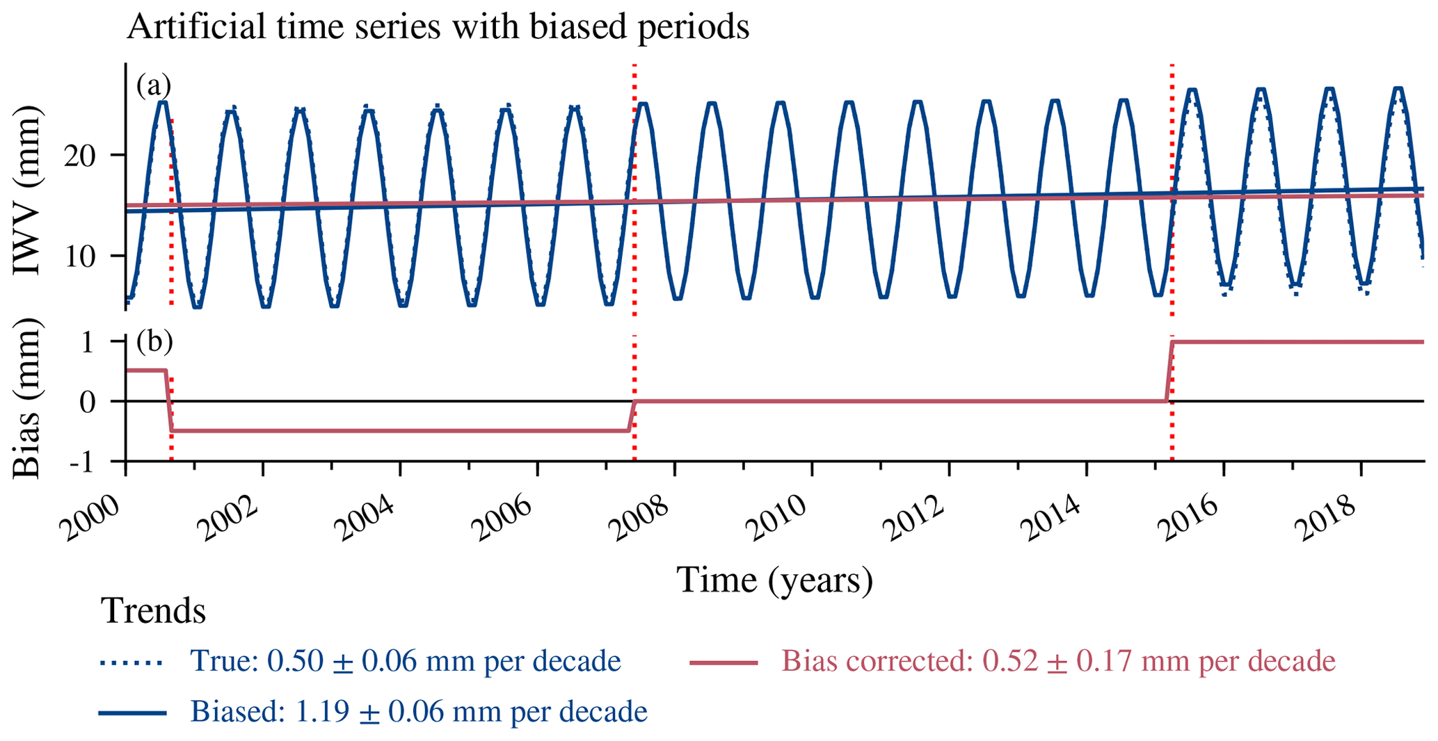
Figure 2Artificial time series (a) and added biases (b). The linear trends for the true (unbiased) data, the biased data and the bias-corrected data are given with 1-standard-deviation uncertainties.
3.1.2 Bias fitting for GNSS trends
In the present study, we use the bias fitting on GNSS data sets to account for instrumental changes. Analysing IWV trends from GNSS data is challenging because the measurements are highly sensitive to changes in the setup (mainly concerning antennas and radomes, but also receivers and cables) or in the environment (Pacione et al., 2017). The presented method is a straightforward way to obtain reliable IWV trend estimates despite possible data jumps due to instrumental changes. We consider each instrumental change in the trend programme, requiring as single information the dates when changes have been performed at the GNSS stations and an estimate of the bias uncertainty. We introduced change points in the trend programme as soon as a possible jump in the GNSS height data was recorded by swisstopo (available at http://pnac.swisstopo.admin.ch/restxt/pnac_sta.txt, last access: 12 July 2019), which was mostly due to antenna updates.
After such antenna changes, we assume a bias uncertainty of 5 % of the averaged IWV value for each biased subset. The bias uncertainty of 5 % was chosen based on our example case at Neuchâtel (Fig. 3), in which we observed a bias of 4 % after an antenna change. This is also consistent with results from Gradinarsky et al. (2002) and Vey et al. (2009), who found IWV jumps of around 1 mm due to antenna changes or changes in the number of observations and the elevation cut-off angles. For a typical Swiss station with averaged IWV values of around 16 mm, this corresponds to a bias of around 6 %. Ning et al. (2016b) found IWV biases due to GNSS antenna changes mostly between 0.2 and 1 mm, which corresponds to a bias of 1 % to 6 %, confirming our choice of 5 % bias uncertainty. In addition to the antenna updates, we added change points in the GNSS time series when a new antenna and receiver was added to replace an older system nearby (see Table 1). This can lead to larger biases, and we therefore assume a bias uncertainty of 10 % due to this data merging. For some antenna updates, jumps were observed back to a data level of a previous period. These subsets were then considered as unbiased to each other. Otherwise, we assumed the longest data block to be the unbiased reference block.
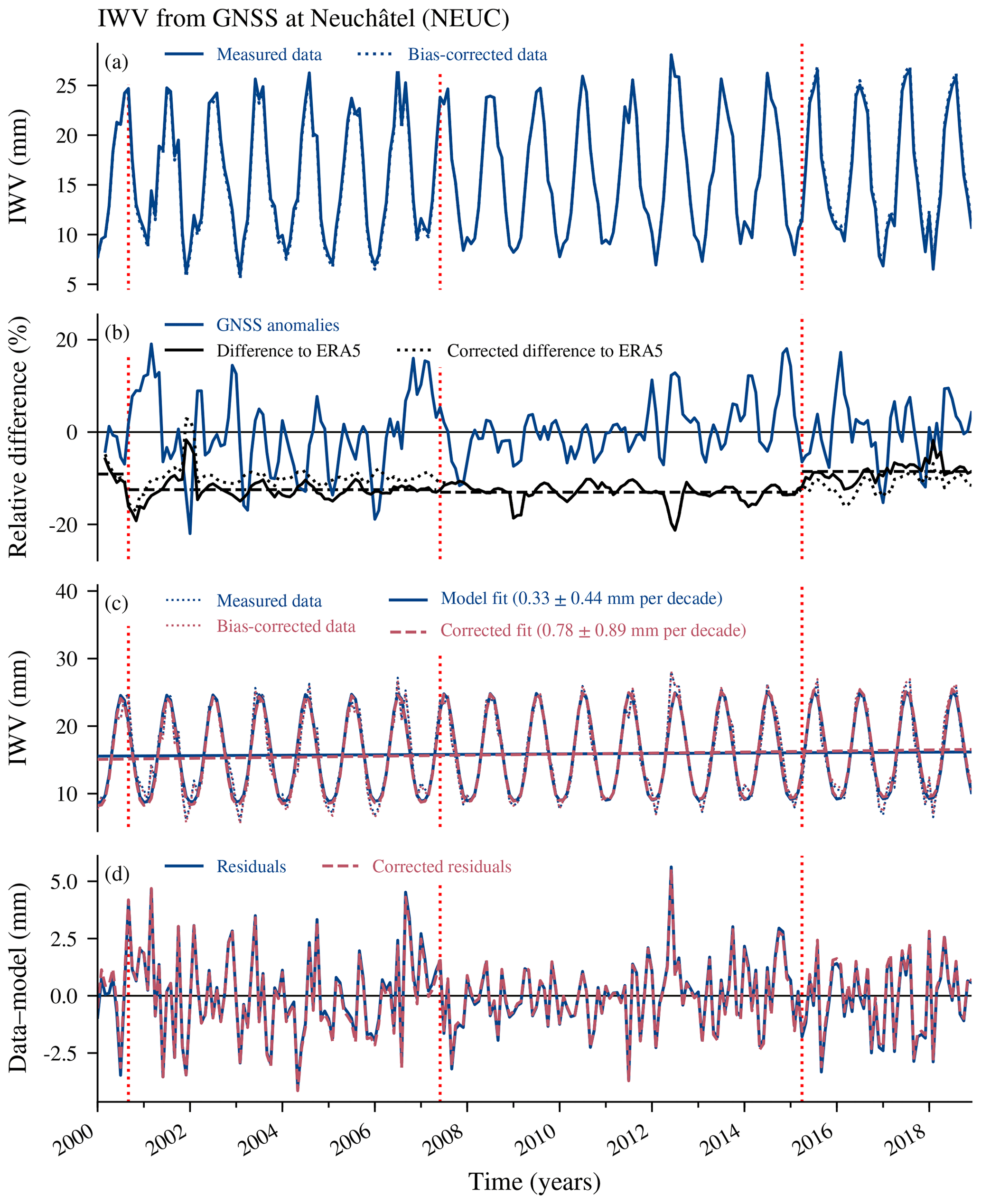
Figure 3(a) Monthly means of integrated water vapour (IWV) from the GNSS station at Neuchâtel (NEUC), Switzerland. Changes in antenna types are indicated in all panels by vertical red dotted lines. (b) Anomalies from the climatology ((data − climatology) ∕ climatology) of the GNSS data at Neuchâtel and relative difference compared to ERA5 data at the same location ((ERA5 − GNSS) ∕ GNSS), both smoothed with a 3-month moving mean window. The horizontal black dashed lines show the averaged difference compared to ERA5 for each antenna change. The relative difference of the bias-corrected GNSS data to ERA5 is also shown (dotted line). (c) Regression model fit and (d) residuals of the model without bias correction and with correction by considering data jumps in the trend model. The given trend uncertainties correspond to 2 standard deviations (σ).
The trend programme and the bias correction are illustrated by an example case of the GNSS station in Neuchâtel, Switzerland (Fig. 3). Figure 3a shows the monthly IWV time series of GNSS data in Neuchâtel with antenna updates in the years 2000, 2007 and 2015 (vertical red dotted lines). Figure 3b shows the deseasonalized anomalies of the IWV time series, divided by the overall mean value of each month, illustrating the interannual variability. The anomalies are less variable from 2007 to 2012, but it is not clear whether this is related to the antenna update in 2007. Furthermore, the relative difference compared to ERA5 () reveals a data jump after the antenna change in 2015 (Fig. 3b). After this antenna update to multi-GNSS, the mean difference compared to ERA5 was reduced, suggesting that the antenna update improved the measurements. The jump corresponds to a bias in IWV of 0.66 mm (4 %) compared to the data before the change. Such a jump can falsify the resulting trend. In the corrected trend fit, the trend model therefore accounts for possible biases for each antenna update. When the bias is considered in the trend model, the jump in the difference compared to ERA5 is reduced (Fig. 3b). Furthermore, we obtain a larger bias-corrected trend (0.78±0.89 mm per decade) compared to the trend of the initial data (0.33±0.44 mm per decade) (Fig. 3c and d), suggesting that IWV was overestimated in earlier years. In general, the trend fit (Fig. 3c) reproduces the IWV time series well. For both model fits, 90 % of the residuals (Fig. 3d) lie within 2 mm, which corresponds to differences between observed data and model fit below 17 %. The regression model explains 93 % of the variability of the IWV time series at this station. As described above, the resulting trend depends on the assumed bias uncertainties and random observational error. However, respective tests have shown that different observation error covariance matrices, where these quantities were varied within realistic bounds, lead to trend estimates within the error margin of the original trend estimate.
IWV measurements from the TROWARA radiometer in Bern are compared to surrounding GNSS stations and reanalysis data. Figure 4 shows monthly means of TROWARA and reanalyses, as well as the averaged monthly means of seven GNSS stations close to Bern. The selected GNSS stations lie within ±0.5∘ latitude and ±1∘ longitude around Bern, with a maximum altitude difference of 200 m (see Table 1). The altitude restriction has been chosen to avoid the inclusion of the two higher-altitude stations (Zimmerwald and Bourrignon) that are close to Bern but show larger IWV variability due to their higher elevation.

Figure 4(a) Monthly means of IWV from the microwave radiometer TROWARA in Bern (Switzerland), from GNSS stations close to Bern and from reanalysis grids (MERRA-2 and ERA5) at Bern. (b) Anomalies from the climatology ((data − climatology)∕climatology) for each of the mentioned data sets. (c) Relative differences of the mentioned data set X to TROWARA (T) data (). The bold lines in (b) and (c) show the data smoothed with a moving mean window of 3 months; the thin pale lines show the unsmoothed monthly data.
Generally, we observe a good agreement between the data sets, with interannual variability that is captured by all data sets (Fig. 4b). The data sets agree well with TROWARA, with averaged differences smaller than 0.6 mm (∼5 %). Only the stations in Bern (WAB1 and EXWI) show a bias compared to TROWARA (not shown). The Huttwil (HUTT) station reports less IWV than TROWARA, which is probably due to the higher station altitude. The GNSS stations around Bern agree well with TROWARA after 2013 and show larger winter differences before 2008 (Fig. 4c).
ERA5 agrees generally well with TROWARA, whereas MERRA-2 differs slightly more. Especially in the last decade, the MERRA-2 difference compared to TROWARA shows a strong seasonal behaviour with larger differences in winter, which is not visible in the other data sets. Correcting the reanalysis data for a possible altitude mismatch due to wrong topography assumptions (Bock and Parracho, 2019) might partly reduce discrepancies between reanalyses and observations.
4.1 IWV trends around Bern
Trends of IWV for the different data sets around Bern are shown in Fig. 5 and Table 2. IWV measured by the radiometer TROWARA increased significantly by 4.8 % per decade from 1995 to 2018. This trend value is similar to the bias-corrected trends from GNSS stations in Lausanne (EPFL), Huttwil (HUTT), Lucerne (LUZE), Neuchâtel (NEUC) and Wabern next to Bern (WAB1), which all report trends around 5 % per decade (Fig. 5 and Table 2). We observe a slightly larger trend in Payerne (PAYE, 7.0 % per decade). The GNSS station in Bern, located on the roof of the university building of exact sciences (EXWI), shows a trend of nearly zero (0.1 % per decade). Unfortunately, the site EXWI has not been operation since September 2017. Reanalysis IWV at Bern increases significantly by 3.7 % per decade for MERRA-2 and by 2.3 % per decade for ERA5 data, both for the period from 1995 to 2018. With the exception of Payerne, all GNSS trends are not significantly different from zero at the 95 % confidence interval. The larger GNSS trend uncertainties compared to TROWARA and reanalysis trends are mainly due to the bias correction, which adds some uncertainty to the trend estimates. Furthermore, all GNSS trends result from a shorter time period than TROWARA and reanalysis trends (see Table 1), which also increases the trend uncertainty and may lead to some trend differences. For comparison, the GNSS trends without bias correction are also shown in Table 2. They are generally smaller than the bias-corrected trends, suggesting that GNSS trends are mostly underestimated when biases are not accounted for. Furthermore, their uncertainties are smaller, reflecting the additional uncertainty when biases are considered.
Table 2IWV trends for TROWARA in Bern, GNSS stations close to Bern and reanalysis grids (MERRA-2 and ERA5) at Bern, with 2 σ uncertainties. GNSS trends have been bias corrected in the case of antenna updates. The uncorrected trends for these stations are given in brackets. Trends that are significantly different from zero at the 95 % confidence interval are shown in bold.
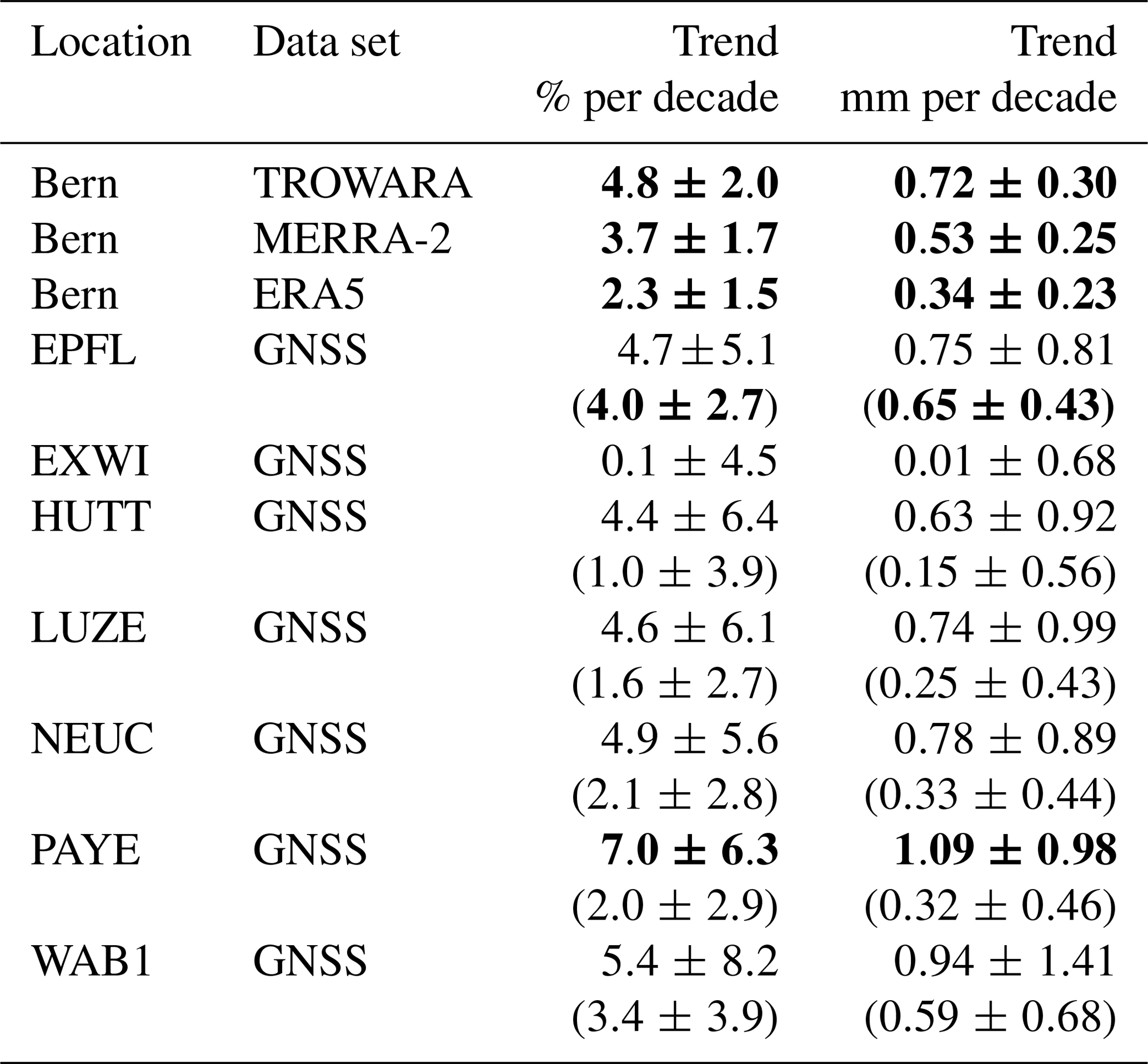
In brief, most of the GNSS stations around Bern report positive trends of approximately 5 % per decade. However, two of the GNSS stations around Bern (EXWI and PAYE) report different trends. The near-zero trend at the EXWI station is less reliable than the other trends because the EXWI station is not part of the AGNES network and therefore does not fulfil the same quality requirements. The large GNSS trend in Payerne results from the bias correction. If the bias correction in the trend fit (as described in Sect. 3) is not applied, the trend in Payerne is only 2 % per decade (0.32 mm per decade), whereas it increases to 7.0 % per decade (1.09 mm per decade) when accounting for antenna changes. Nyeki et al. (2019) found IWV trends in Payerne from GNSS measurements of 0.8 mm per decade, which lie between our corrected and uncorrected trends. This suggests that the instrumental changes in Payerne play an important role but might be overcorrected in our case. The recent study by Hicks-Jalali et al. (2020) reports similar IWV trends in Payerne using nighttime radiosonde measurements (6.36 % per decade) and even larger trends using clear-night lidar data (8.85 % per decade) in the period from 2009 to 2019, suggesting that IWV in Payerne was strongly increasing, especially in recent years. However, comparing their trend results with ours has to be done with care, because their trend time period is short and the lidar trends might contain a clear-sky bias.

Figure 5IWV trends for TROWARA in Bern, reanalysis (MERRA-2 and ERA5) grid points at Bern and GNSS stations close to Bern. The error bars show 2 σ uncertainties. Filled dots represent trends that are significantly different from zero at the 95 % confidence interval.
The trend from the TROWARA radiometer of 4.8 % per decade (0.72 mm per decade) slightly differs from the TROWARA trends reported by Morland et al. (2009) and Hocke et al. (2011, 2016). It is larger than TROWARA's 1996 to 2007 trend of 3.9 % per decade (0.56 mm per decade) (Morland et al., 2009). Hocke et al. (2011) found no significant TROWARA trend for the period 1994 to 2009, which suggests that our larger IWV trends are mainly due to a strong IWV increase in the last decade. This is also confirmed by Hocke et al. (2016), who observed larger trends for recent years (1.5 mm per decade for 2004 to 2015). However, care has to be taken when comparing these TROWARA trends of different trend period lengths.
To summarize, IWV trends around Bern from TROWARA and GNSS data generally lie around 5 % per decade, whereas reanalysis trends for the Bern grid are slightly smaller.
Seasonal IWV trends around Bern
To study the seasonal differences of the IWV trends around Bern, we analysed trends for each month of the year (Fig. 6). The absolute trends (Fig. 6a) are largest in summer months due to more IWV in summer. The trends in percent (Fig. 6b) account for the seasonal cycle in IWV, leading to more uniform trends throughout the year. However, differences between winter trends might sometimes be overweighted when calculating trends in percent: a small trend difference in winter will be more important when expressed in percent than the same difference in summer trends because of less water vapour in winter. Nevertheless, we will concentrate on trends in percent per decade in the following, which facilitates comparing relative changes in IWV in different seasons.

Figure 6Trends of IWV for different months for TROWARA in Bern, GNSS stations close to Bern (arithmetic mean) and reanalysis grids (MERRA-2 and ERA5) at Bern. Uncertainty bars show the maximum range of 2 σ uncertainties of each data set. Filled dots represent trends that are significantly different from zero at the 95 % confidence interval. Monthly IWV trends are given in (a) as absolute trends in millimetres per decade and in panel (b) as relative trends in percent per decade. Panel (c) presents again the monthly IWV trends from ERA5, as well as the relative humidity (RH) trends and the theoretical change in saturation vapour pressure es due to the observed temperature change from ERA5 data (both averaged below 500 hPa).
Our monthly trends in Bern mostly agree on the largest and significant trends in June (∼7 % per decade to 9 % per decade) and in November (∼8 % per decade to 10 % per decade) as well on minimal but insignificant trends in February and October (Fig. 6b). Furthermore, all data sets report a special pattern of low trends in October, with again larger trends in November. However, the differences between those monthly trends are significant only at the 68 % confidence level. The mean trend (arithmetic mean) of the GNSS stations around Bern agrees with the other data sets in summer but shows an offset to the other trends in several months, especially in March and in autumn. We further found that MERRA-2 trends are slightly larger in summer than trends from the other data sets, whereas TROWARA trends differ from the other trends in the winter months of December and January. This larger disagreement between TROWARA and reanalysis trends in December and January is consistent with the larger winter biases of TROWARA starting in 2008 in Fig. 4c.
Previous studies analysed TROWARA seasonal trends using shorter time periods. Morland et al. (2009) and Hocke et al. (2011) observed significant positive summer trends and negative winter trends for TROWARA. Our TROWARA trends confirm positive summer trends (significant in June and August) but do not confirm negative winter trends. The observed autumn peak (minimum trend in October and a trend peak in November) has also been reported by Morland et al. (2009) and Hocke et al. (2011). However, their trend peak was shifted by 2 months, with a minimum in August and a subsequent maximum in September. The 10 additional years that we use in our study compared to their data might be responsible for this shift. Morland et al. (2009) proposed that this autumn trend peak might be related to precipitation changes, but such a relationship has not been verified for the present study. Nevertheless, we showed that the IWV trend peak is consistent with November temperature trends, suggesting that those trends are temperature driven (see Sect. 4.2 and Fig. 6c).
In summary, Bern data sets generally agree on the annual trend distribution, with the largest trends in June and in November. However, the monthly trends of GNSS stations around Bern disagree with the other data sets in spring and in autumn, whereas TROWARA deviates in December and January. Positive summer trends are reported by all data sets.
4.2 Changes in IWV and temperature around Bern
To examine the relationship between IWV trends and changing temperature, we present the theoretical change in water vapour in the atmosphere due to observed changes in temperature (Fig. 6c). For this, we determined the temperature-dependent change in saturation vapour pressure for the time period 1995 to 2018. The saturation vapour pressure es describes the equilibrium pressure of water between the condensed and the vapour phase. It increases rapidly with increasing temperature (Held and Soden, 2000). In cases where the water vapour pressure e is smaller than es, the available water is in the vapour phase, whereas for e≥es it condenses. With increasing temperature, es increases, which leads to an increase in e for a given relative humidity (RH). Changes in es can therefore directly be compared to changes in the amount of water vapour, assuming that RH remains constant (Möller, 1963; Held and Soden, 2000):
A change in es is then directly reflected in a change in e and therefore in IWV:
The fractional change in es for a given change in temperature can be approximated by the Clausius–Clapeyron equation:
where Lv is the latent heat of evaporation (), Rv is the gas constant for water vapour (), dT is the change in temperature and T is the actual temperature. To obtain the tropospheric temperature change dT, we derived the temperature trend (1995 to 2018) from ERA5 temperature profiles, averaged below 500 hPa. This limit was chosen because around 95 % of IWV resides below 500 hPa for the averaged ERA5 profiles in our study period. The resulting temperature trend (in kelvin per decade) is then used for dT in Eq. (13) to determine the change in es in percent per decade. For the actual temperature T we used the mean of ERA5 temperature profiles below 500 hPa for the same time period.
The fractional changes in ERA5 es for the Bern grid for different months are shown in Fig. 6c. These temperature-induced changes in es agree generally well with the observed trends in IWV. They agree especially well with TROWARA and reanalysis trends in spring (March and April), late summer and autumn (July to November), but they agree less in the winter months and in May and June. Furthermore, they agree less with GNSS trends from September to March. Generally, the good agreement between the change in es and the IWV trends indicates that observed IWV changes around Bern can mostly be explained by temperature changes. However, the changes in es do not confirm our observed IWV winter trends, especially in January and February. This discrepancy can be related to changes in RH, which was assumed to be constant (Eq. 11). Indeed, our trends of ERA5 RH for the Bern grid (Fig. 6c) show that RH was not constant in those months, especially in winter but also in May and June. Even though the RH trends are not significantly different from zero, these results suggest that assuming RH to be constant may not be valid during all seasons, especially in winter. This makes the attribution of IWV trends to changes in temperature more challenging. Furthermore, other factors than temperature might be responsible for IWV changes in winter, such as changes in dynamical patterns and the horizontal transport of humid air. Indeed, Hocke et al. (2019) showed that evaporation of surface water plays a minor role in winter, with a latent heat flux that is 6 to 7 times smaller than in summer in Bern, suggesting that, in winter, horizontal transport of humid air is more important than evaporation.
We conclude that IWV in Bern changes as expected from temperature changes in early spring, late summer and autumn, but other processes might also be responsible for IWV changes, especially in winter.
We compare IWV at Jungfraujoch from a GNSS antenna and an FTIR spectrometer (Fig. 7). Due to the sparser FTIR sampling, we compare FTIR data not only with the full GNSS time series, but also with coincident GNSS data, i.e. pairwise data limited to clear-sky weather conditions. Monthly means of these sparser data have been computed by a seasonal fitting as described in Sect. 2.2. This leads to some missing data at the edges of the coincident GNSS time series (Fig. 7a, c) because a specific number of data points is required for the seasonal fitting. For the FTIR time series, no data are missing at the edges because data were available beyond the dates of our study period.
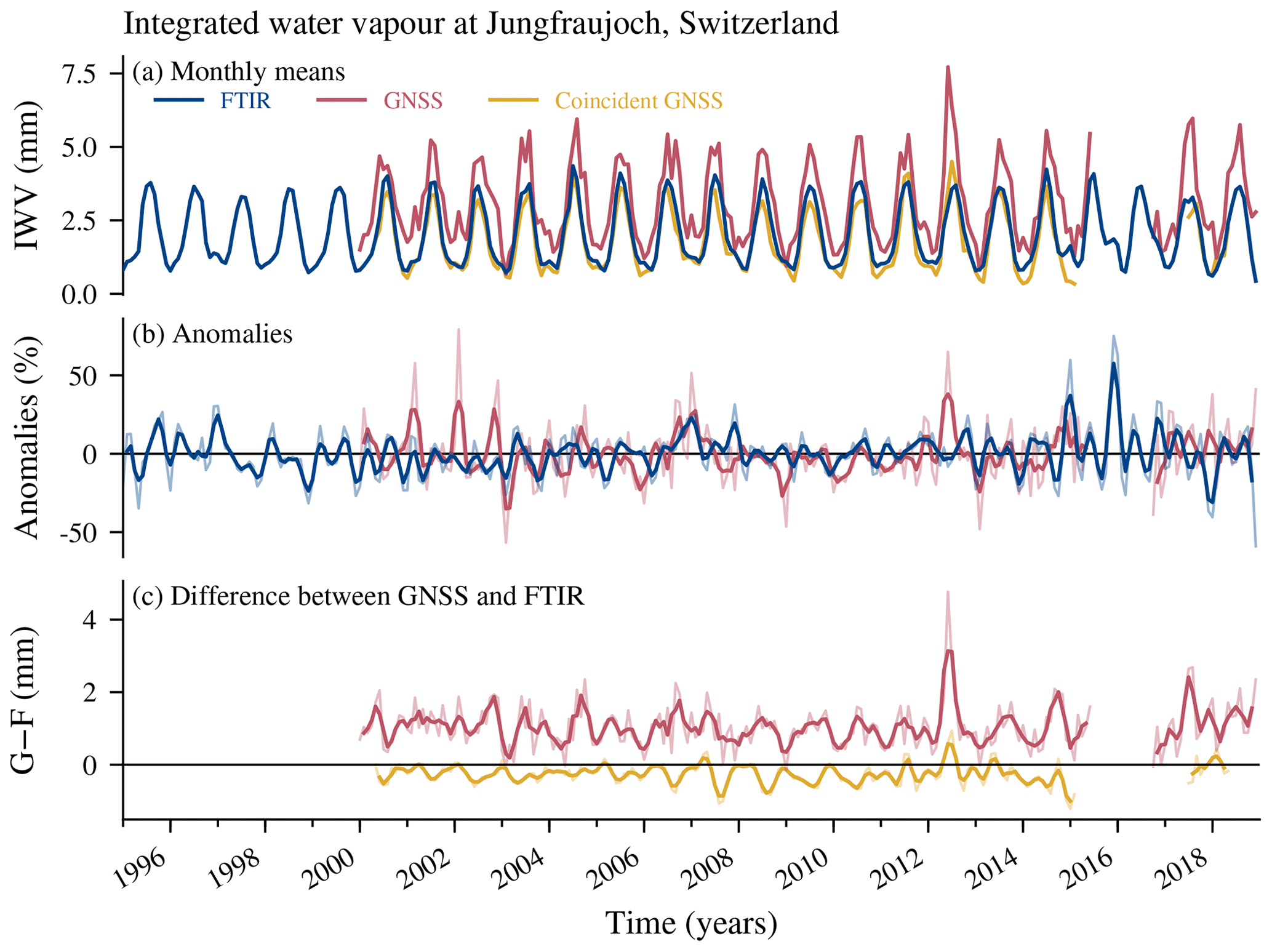
Figure 7(a) Monthly means of IWV from the FTIR spectrometer and the GNSS station at Jungfraujoch (Switzerland). Shown are GNSS means once using the full hourly sampling and once using data only at the same time as the FTIR measured (coincident GNSS). The monthly means of FTIR and coincident GNSS have been resampled to correspond to the 15th of each month. (b) Anomalies from the climatology ((data − climatology)∕climatology) for FTIR data and fully sampled GNSS data. (c) Differences between GNSS (G) and FTIR (F) data, using the full GNSS data and GNSS data coincident with the FTIR. The bold lines in (b) and (c) show the data smoothed with a moving mean window of 3 months; the thin pale lines show the unsmoothed monthly data.
We observe less IWV at Jungfraujoch than at Bern due to the high altitude of the station, with a mean IWV from GNSS of 3 mm (Fig. 7a). The deseasonalized anomalies (Fig. 7b) show that the interannual variability of IWV at Jungfraujoch is larger than in Bern, with anomalies larger than 50 % for some months. Monthly means of coincident GNSS data have a mean dry bias of mm compared to FTIR (GNSScoincident−FTIR) (Fig. 7c). This corresponds to a bias of 15 % when referring to the long-term average of GNSS coincident IWV data. Furthermore, monthly means of fully sampled GNSS have a bias of 1.05±0.61 mm compared to FTIR (GNSS−FTIR), which corresponds to a bias of 34 % (using the mean of the fully sampled GNSS as reference). This larger bias illustrates the sampling effect of the FTIR measurements, leading to a dry bias of FTIR compared to GNSS data. Indeed, the difference results from the restriction that FTIR measurements require clear-sky conditions, preventing measurements during the wettest days.
The remaining bias of −0.26 mm when using coincident GNSS measurements indicates that GNSS measures slightly less IWV than FTIR. This is consistent with results from Schneider et al. (2010), who report that GNSS at the high-altitude Izaña Observatory (Tenerife) systematically underestimates IWV in dry conditions (<3.5 mm). Furthermore, a dry bias has also been observed in previous studies that compared Jungfraujoch GNSS data with precision filter radiometer (PFR) data (Guerova et al., 2003; Haefele et al., 2004; Nyeki et al., 2005; Morland et al., 2006). Guerova et al. (2003) attributed this bias to incorrect modelling of the antenna phase centre and Haefele et al. (2004) to unmodelled multi-path effects of the Jungfraujoch antenna. Brockmann et al. (2019) stated that the old GPS-only antenna used at Jungfraujoch until 2016 was never calibrated. Due to the special radome construction (with circulating warm air to avoid icing), the standard antenna phase centre calibration is not appropriate for use with the Jungfraujoch data. From this point of view the achieved results are good and a possible offset is not relevant for trend analyses as long as it is constant over the whole trend period. The use of this antenna was stopped in summer 2015, and it was replaced by a new multi-GNSS antenna in October 2016 (Brockmann et al., 2016). Furthermore, the complete antenna-radome construction was individually calibrated for GPS and GLONASS signals (Galileo and BeiDou are assumed to be identical to GPS). We found that the bias to FTIR has been reduced to −0.07 mm ± 0.28 (4 %) after the antenna change in 2016, suggesting that the GNSS antenna update improved the consistency of the measurements at Jungfraujoch.
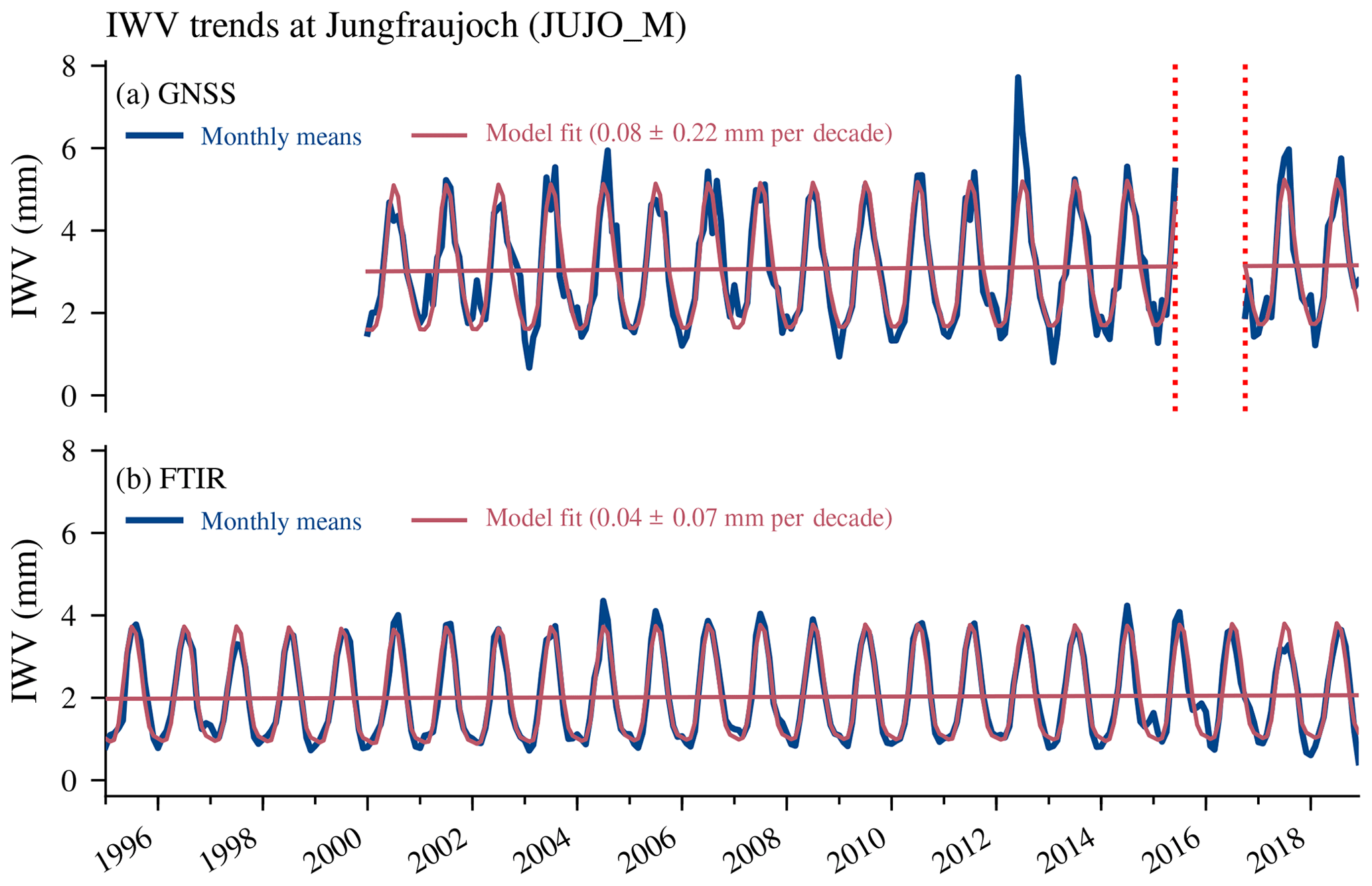
Figure 8Monthly means and their trend fits for (a) GNSS and (b) FTIR data at Jungfraujoch. The given trend uncertainty corresponds to 2 σ uncertainties. GNSS antenna changes are indicated by vertical red dotted lines.
IWV trends at Jungfraujoch
The IWV trends at the Jungfraujoch station from FTIR and fully sampled GNSS data are presented in Fig. 8. The GNSS antenna update has been considered in the trend estimate as described in Sect. 3.1.2. We observe IWV trends of 0.08 mm per decade (2.6 % per decade) for GNSS and 0.04 mm per decade (1.8 % per decade) for FTIR. However, both trends are insignificant. The difference between both trends can partly be explained by the dry sampling bias of the FTIR spectrometer, which measures only during clear-sky day conditions. Indeed, the absolute GNSS trend is comparable with the FTIR trend when we use GNSS data coincident with FTIR measurements, with 0.05 mm per decade (not shown). Our IWV trends at Jungfraujoch are similar to the trend by Sussmann et al. (2009), who reported insignificant FTIR trends at the same station of 0.08 mm per decade in the time period 1996 to 2008. In contrast to these results, Nyeki et al. (2019) found larger trends at Jungfraujoch that were significantly different from zero. They decided not to use GNSS IWV data from Jungfraujoch due to the high IWV variability and the missing calibration of the antenna before the replacement in 2016. Therefore, they derived their trends from IWV data based on a parameterization from surface temperature and relative humidity measurements. However, they admit that this approximation is prone to large uncertainties (Gubler et al., 2012), which might explain parts of the differences compared to our trends.
6.1 Swiss GNSS trends
The GNSS data generally report positive IWV trends throughout Switzerland (Fig. 9). Using data for the whole year (Fig. 9a), 50 % of the stations show trends between 2.3 % per decade and 5.1 % per decade (0.27 and 0.74 mm per decade). The trends of all stations range between 0.1 % per decade and 7.2 % per decade (0.01 mm per decade and 1.09 mm per decade), with exception of three stations that show negative trends (ANDE, HOHT and MART_M). The mean trend value of all GNSS stations is 3.6 % per decade (0.49 mm per decade), and the median is 4.4 % per decade (0.57 mm per decade).
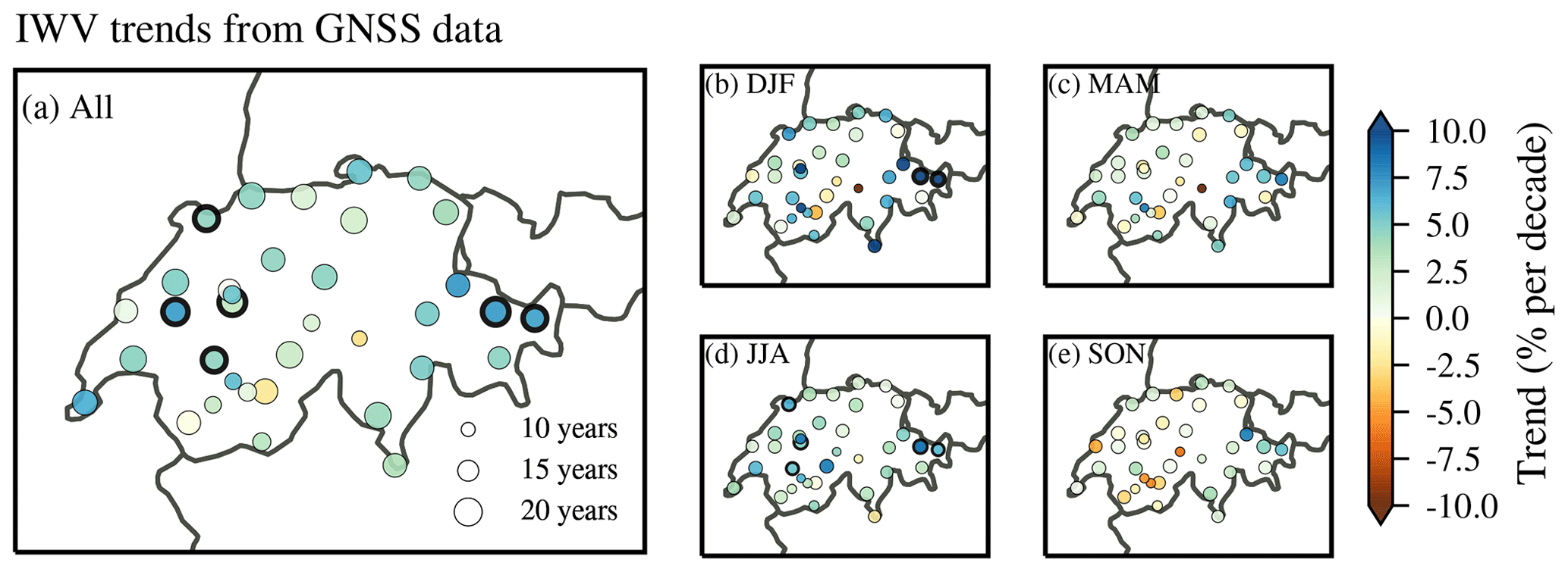
Figure 9Trends of IWV in Switzerland for the different GNSS stations for (a) the whole year, (b) winter (December, January, February), (c) spring (March, April, May), (d) summer (June, July, August) and (e) autumn (September, October, November). The length of the GNSS time series (Table 1) is indicated by the size of the markers. Stations with trends that are significantly different from zero at the 95 % confidence interval are marked with a bold edge.
Only three stations (9 % of all stations) show negative IWV trends and none of them is significantly different from zero at the 95 % confidence interval. Significant positive trends are reported at 17 % of the stations (six stations), being generally stations with long time series and lying mostly in western and south-eastern Switzerland. Most significant trends are observed in summer (Fig. 9d), with significant positive trends at five stations. In winter, only two north-eastern Swiss station trends are significant (Fig. 9b). In spring (Fig. 9c) and autumn (Fig. 9e), none of the IWV trends are significantly different from zero. Autumn trends tend to be negative, especially in the south-western part (Rhône valley in the canton of Valais), but they are all insignificant.
Our trend range covered by all GNSS stations is consistent with results from Nilsson and Elgered (2008), who observed in Sweden and Finland IWV trends between −0.2 and 1 mm per decade. However, they concluded that their study period was too short (10 years) to obtain stable trends. Our trends also lie within the range of trends observed in Germany by Alshawaf et al. (2017). Their trends vary even more between different stations, with trends ranging between −1.5 and 2.3 mm per decade. Note, however, that both studies use different trend period lengths than in our study, which makes trend comparisons difficult. The recent study by Nyeki et al. (2019) reports IWV trends from GNSS data at three Swiss stations for the period 2001 to 2015. Using Sen's slope trend method, they found positive all-sky trends in Davos (0.89 mm per decade), Locarno (0.42 mm per decade) and Payerne (0.80 mm per decade).
Our GNSS trends for these stations are slightly different (Davos: 0.71 mm per decade, Locarno: 0.72 mm per decade, Payerne: 1.09 mm per decade), which might be due to the three additional years in our analysis, but also due to our bias correction in the trend model. Furthermore, our GNSS-derived ZTD data were reprocessed until 2014 (see Sect. 2.3), whereas Nyeki et al. (2019) still used the old GNSS data.
Note that most bias-corrected GNSS trends are larger than the uncorrected trends. This suggests that earlier GNSS data overestimate IWV compared to recent measurements. A possible explanation might be the enhancement from GPS-only to multi-GNSS antennas that was performed on AGNES stations in spring 2015. In our example case (Fig. 3b), this update improved GNSS IWV measurements compared to ERA5 data, suggesting that IWV was overestimated by GNSS in earlier years. This overestimation would then lead to a smaller trend, whereas the trend would increase when the jump is corrected in the trend estimation.
The altitude dependence of the GNSS trends is shown in Fig. 10. We observe that most of the stations that show significant positive trends lie at higher altitudes. Indeed, 83 % of the stations showing significant trends lie at altitudes above 850 m a.s.l., whereas less than half of the stations lie above 850 m. This is consistent with the expectation of Pepin et al. (2015) that the rate of warming is larger at higher altitudes. Due to the direct link between temperature and water vapour content, an increased warming at higher altitudes would lead to larger IWV trends. The increasing significance with altitude provides some observational evidence for this suggestion. However, the altitude dependence is less visible in absolute trends (not shown), which indicates that, due to less IWV at higher altitudes, these trends are more sensitive to changes when calculating trends in percent. Also, the IWV trends of the six stations with highest altitudes (>1650 m a.s.l.) are not significantly different from zero.
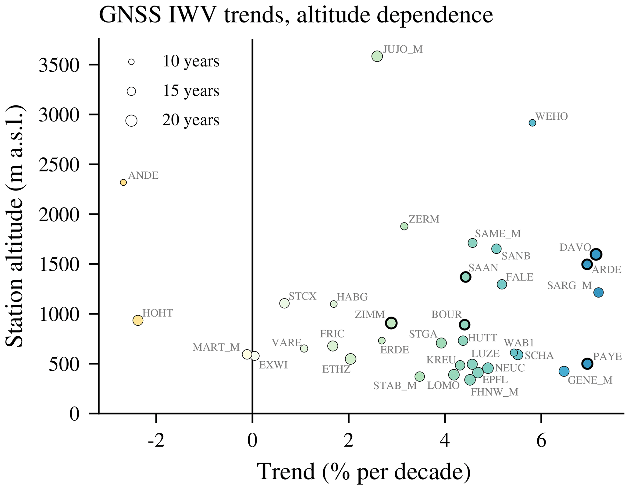
Figure 10IWV trends from GNSS stations in Switzerland with the station altitude. For merged stations (see Table 1), the averaged altitude of both stations is used. The colours correspond to the trend in percent per decade and are the same as in Fig. 9; the length of the time series is indicated by the size of the markers. Trends that are significantly different from zero are shown with bold edges. The station abbreviations are explained in Table 1.
We conclude that Swiss GNSS stations generally show positive IWV trends, with a mean value of 3.6 % per decade (0.49 mm per decade) and a tendency for more significant percentage trends at higher altitudes.
6.2 Swiss reanalysis trends
Reanalysis trends of IWV for Switzerland are presented in Figs. 11 and 12. The trends are on average 2.6 % per decade (0.35 mm per decade) for ERA5 (Fig. 11a) and 3.6 % per decade (0.52 mm per decade) for MERRA-2 (Fig. 12a). Both reanalysis trends show only small spatial variability. The seasonal trends are positive, with the largest values in summer (Figs. 11d and 12d). This is consistent with our observed GNSS trends, which are mostly positive in summer. The smallest and partly negative reanalysis trends are observed in winter (Figs. 11b and 12b), which contrasts with our GNSS trends that showed the smallest (but insignificant) trends in autumn and not in winter. In spring and autumn, the reanalysis trends are spatially more variable. Both data sets report slightly larger autumn trends in south-eastern Switzerland and northern Italy (Figs. 11e and 12e). In spring, ERA5 shows larger IWV trends in south-western Switzerland.

Figure 11IWV trends from ERA5 reanalysis data in Switzerland from 1995 to 2018 for the whole year (a) and for the different seasons (b to e). GNSS trends are additionally shown in panel (a) (same as in Fig. 9a but restricted to stations with longest time series of 18 and 19 years).
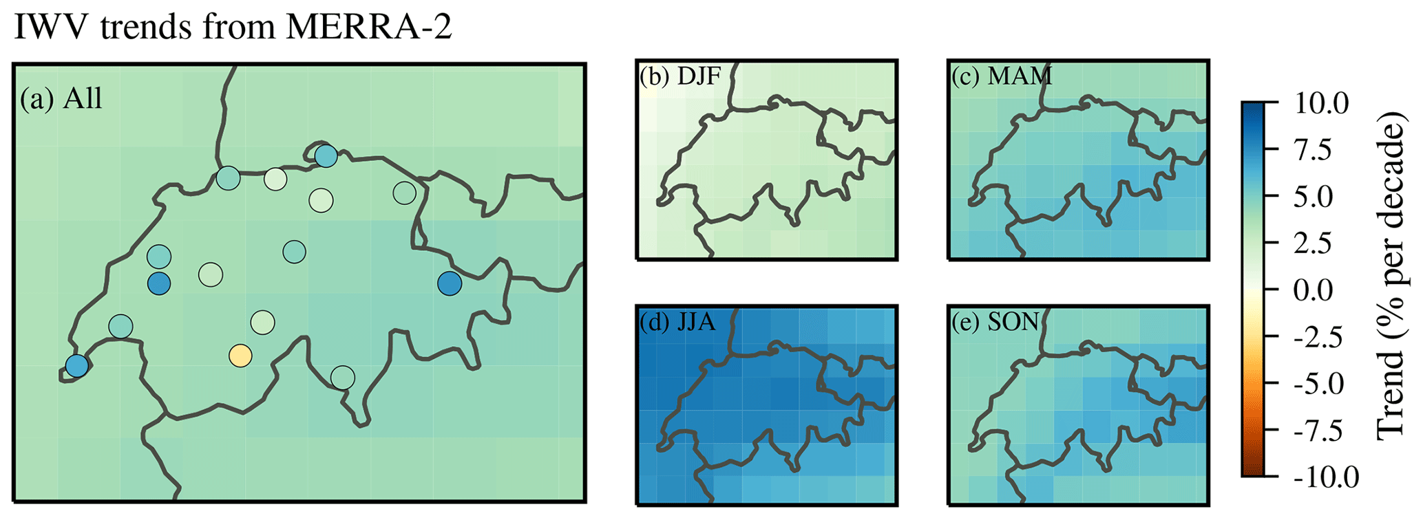
Figure 12Same as Fig. 11 but for MERRA-2 reanalysis data (1995–2018).
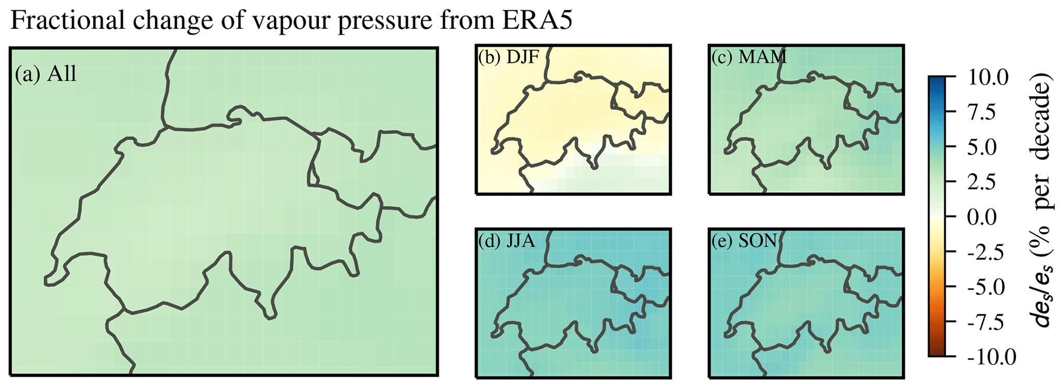
Figure 13Fractional change in water vapour pressure (es) derived from temperature trends from ERA5 (1995–2018) for the whole year (a) and different seasons (b to e). The temperature data were averaged below 500 hPa.
The averaged MERRA-2 trend agrees with our averaged GNSS trend (both 3.6 % per decade), which is slightly larger than the averaged ERA5 trend (2.6 % per decade). However, the reanalyses do not resolve small-scale variability, which can explain the differences compared to some GNSS station trends. Furthermore, the GNSS point measurements are generally more variable than the gridded reanalyses data. Alshawaf et al. (2017) also observed larger differences in mountainous regions between GNSS-derived IWV and reanalyses data in Germany. Our mean ERA5 trend for Switzerland of 0.35 mm per decade is consistent with IWV trends from ERA-Interim in Germany reported by Alshawaf et al. (2017) (0.34 mm per decade). The MERRA-2 trends are generally slightly larger than the ERA5 trends. Parracho et al. (2018) also found larger IWV trends for MERRA-2 compared to ERA-Interim reanalysis trends on a global scale, especially in summer.
To determine the relationship between temperature changes and IWV trends for the whole of Switzerland, we present changes in saturation vapour pressure es derived from ERA5 temperature changes below 500 hPa (as described in Sect. 4.2). The fractional change in ERA5 es, which corresponds to the change in IWV (Eq. 12), is presented in Fig. 13. The averaged changes in ERA5 es of 2.9 % per decade are similar to our ERA5 IWV trends described before (2.6 % per decade), which indicates that IWV is on average following the temperature change as expected from the Clausius–Clapeyron equation. The ERA5 es changes are spatially more uniform than the ERA5 IWV trends but agree well in all seasons, except in winter (Figs. 13b and 11b). ERA5 es is decreasing in winter, whereas ERA5 IWV winter trends are increasing. These conflicting results indicate that factors other than temperature might dominate IWV changes in winter, as already discussed in Sect. 4.2. Furthermore, it indicates that the assumption of constant relative humidity might not be valid in winter. This is confirmed by the ERA5 RH trends (Fig. 14), which are around zero for the whole of Switzerland in all seasons but slightly positive in winter. Even though these positive winter RH trends are not significantly different from zero, they raise the question of whether it is justified to assume RH to be constant.

Figure 14Relative humidity (RH) trends from ERA5 reanalysis data in Switzerland from 1995 to 2018 (averaged below 500 hPa) for the whole year (a) and for the different seasons (b to e).
The partly negative winter changes in es are surprising because they result from a decrease in reanalysis winter temperature. Such a decrease in winter temperature is not consistent with long-term temperature observations in Switzerland, which report a temperature increase also in winter (Begert and Frei, 2018). This difference is due to our short study period. A few cold winters in the past 15 years have hidden the overall positive temperature trend when looking only at the relatively short period from 1995 to 2018 (MeteoSwiss, Federal Institute for Meteorology and Climatology, 2019).
To summarize, the ERA5 IWV trends follow on average the changes expected from temperature changes. The reanalysis IWV trends generally agree well with GNSS trends in Switzerland, but the spatial trend variability is not resolved by the reanalyses. Local measurements of IWV such as microwave radiometer, FTIR or GNSS measurements are therefore crucial to monitor changes in IWV, especially in mountainous regions such as Switzerland.
Our study presents trends of integrated water vapour (IWV) in Switzerland from a ground-based microwave radiometer, an FTIR spectrometer, GNSS stations and reanalysis data. We found that IWV generally increased by around 2 % per decade to 5 % per decade from 1995 to 2018. Using a straightforward trend approach that accounts for jumps due to instrumental changes, we found significant positive IWV trends for some GNSS stations in western and eastern Switzerland. Furthermore, our data show that trend significance tends to be larger in summer and to increase with altitude (up to 1650 m a.s.l.).
Comparing IWV from the radiometer in Bern with GNSS and reanalyses showed a good agreement, with differences within 5 %. The FTIR spectrometer at the high-altitude station Jungfraujoch revealed a constant clear-sky bias of 1 mm compared to GNSS data. Nevertheless, the IWV data and also the trends of both data sets at Jungfraujoch agree within their uncertainties when only coincident measurements are used. We further found that the IWV trends of the Swiss GNSS station network agree on average with the Swiss reanalysis trends (2.6 % per decade to 3.6 % per decade) but that the reanalyses are not able to capture regional variability, especially in the Alps. We conclude that GNSS data are reliable for the detection of climatic IWV trends. However, a few stations may require further quality control and harmonization in the trend analysis.
Measurements in Bern reveal that the IWV trends follow observed temperature changes according to the Clausius–Clapeyron equation. Still, they do not scale to temperature as expected in some months, especially in winter, suggesting that other processes such as changes in dynamical patterns are responsible for IWV changes in winter. However, these winter trends are not significantly different from zero, which prevents us from drawing robust conclusions about temperature-related IWV changes in winter. Also, several colder winters in our study period might hide the long-term winter temperature increase in Switzerland. Nevertheless, ERA5 confirms the departure from Clausius–Clapeyron scaling in winter during our study period.
We did not use lower tropospheric temperature from MERRA-2 in this study because we observed biases in some Alpine grids that we could not explain so far. This reflects the difficulty of using reanalysis data for trend estimates and illustrates that reanalysis data have to be handled with care due to possible changes in observing systems or assimilated data.
Another reason for observed inconsistencies between temperature and IWV changes might be changes in relative humidity (RH). Our temperature–IWV relation assumes that the relative humidity remains constant. However, we found positive RH trends in winter using lower-tropospheric ERA5 data. Even though the RH trends are not significant, they might partly explain the disagreement between observed winter temperature and IWV changes. Wang et al. (2016) states that RH may not be constant because of limited moisture availability over land surfaces. Some studies even found a decrease in relative humidity with increasing temperature at mid-latitudes (O'Gorman and Muller, 2010) or in the subtropics (Dessler et al., 2008). Further analyses with additional data sets would be required to provide more insights into possible RH trends in Switzerland.
It would be necessary to analyse temperature-induced changes at more stations to draw robust conclusions about correlations between temperature and IWV changes. The problem of hidden long-term temperature trends in our study might be solved by using longer temperature time series, but longer IWV time series are sparse. Comparing regional IWV changes with tropospheric temperature changes from observations (e.g. radiosondes) rather than from reanalyses might be another approach to improve understanding of regional temperature–IWV relations. Nevertheless, it is generally difficult to attribute observed climate changes to unambiguous sources and feedbacks (Santer et al., 2007). Only complex attribution studies with multiple model runs can clarify this issue, as done for example by Santer et al. (2007) for IWV over oceans. However, global climate models lack feedbacks on the regional level (Sherwood et al., 2010), and studies based on regional observations are thus necessary.
In summary, our results confirm the increase in water vapour with global warming on a regional scale, stressing the importance of the water vapour feedback. Furthermore, the results emphasize the importance of regional IWV analyses by showing that regional trend differences can be large, especially in mountainous areas. The spatial coverage of long-term IWV measurements from ground stations is sparse. We have shown that homogeneously reprocessed GNSS data have the potential to fill this gap and that they enable monitoring of regional water vapour trends in a changing climate. We further found that water vapour increase follows temperature changes as expected, except in winter. In a changing climate, it is therefore important to assess both regional changes in temperature and water vapour to understand and project possible changes in precipitation patterns and cloud formation on a regional scale.
TROWARA and GNSS-derived IWV data are provided by the STARTWAVE database (http://www.iapmw.unibe.ch/research/projects/STARTWAVE/, STARTWAVE, 2020). The gap-filled TROWARA data used before 2008 are available on request. The Jungfraujoch FTIR data are publicly available from the Network for the Detection of Atmospheric Composition Change (NDACC) at ftp://ftp.cpc.ncep.noaa.gov/ndacc/station/jungfrau/hdf/ftir/ (NDACC, 2019). MERRA-2 data are available online through the NASA Goddard Earth Sciences Data Information Services Center (GES DISC) at https://doi.org/10.5067/KVTU1A8BWFSJ (Global Modeling and Assimilation Office, 2015). ERA5 data are available through the Copernicus Climate Change Service Climate Data Store (CDS) at https://doi.org/10.24381/cds.f17050d7 (Copernicus CDS, 2019a) and https://doi.org/10.24381/cds.6860a573 (Copernicus CDS, 2019b).
The study concept was designed by LB and KH. LB analysed the data and prepared the manuscript. TvC provided the trend programme and GS provided the monthly resampling programme. EM was responsible for the FTIR data, EB for the GNSS data, and CM, NK and KH for the TROWARA data. All co-authors contributed to the manuscript preparation and the interpretation of the results.
The authors declare that they have no conflict of interest.
Leonie Bernet was funded by the Swiss National Science Foundation. We thank the technicians and engineers from the Institute of Applied Physics, University of Bern, who have kept TROWARA working for many years. The University of Liège's involvement has primarily been supported by the F.R.S.–FNRS (Fonds de la Recherche Scientifique) and the Belgian Federal Science Policy Office (BELSPO), both in Brussels, as well as by the GAW-CH programme of MeteoSwiss. The Fédération Wallonie Bruxelles contributed to supporting observational activities. Emmanuel Mahieu is supported by a F.R.S.–FNRS research associate fellowship. We thank the International Foundation High Altitude Research Stations Jungfraujoch and Gornergrat (HFSJG, Bern) for supporting the facilities needed to perform the FTIR observations and the many colleagues who contributed to FTIR data acquisition at that site. The 10.7 cm solar radio flux data were provided as a service by the National Research Council of Canada and distributed in partnership with Natural Resources Canada. Elmar Brockmann from swisstopo provided the GNSS-derived ZTD data (operationally and reprocessed) for all Swiss stations.
This research has been supported by the Swiss National Science Foundation (grant no. 200021-165516).
This paper was edited by Geraint Vaughan and reviewed by two anonymous referees.
Alshawaf, F., Balidakis, K., Dick, G., Heise, S., and Wickert, J.: Estimating trends in atmospheric water vapor and temperature time series over Germany, Atmos. Meas. Tech., 10, 3117–3132, https://doi.org/10.5194/amt-10-3117-2017, 2017. a, b, c, d, e
Armour, K. C., Bitz, C. M., and Roe, G. H.: Time-Varying Climate Sensitivity from Regional Feedbacks, J. Climate, 26, 4518–4534, https://doi.org/10.1175/JCLI-D-12-00544.1, 2013. a
Begert, M. and Frei, C.: Long-term area-mean temperature series for Switzerland–Combining homogenized station data and high resolution grid data, Int. J. Climatol., 38, 2792–2807, https://doi.org/10.1002/joc.5460, 2018. a
Bengtsson, L., Hagemann, S., and Hodges, K. I.: Can climate trends be calculated from reanalysis data?, J. Geophys. Res.-Atmos., 109, D11111, https://doi.org/10.1029/2004JD004536, 2004. a
Bernet, L., von Clarmann, T., Godin-Beekmann, S., Ancellet, G., Maillard Barras, E., Stübi, R., Steinbrecht, W., Kämpfer, N., and Hocke, K.: Ground-based ozone profiles over central Europe: incorporating anomalous observations into the analysis of stratospheric ozone trends, Atmos. Chem. Phys., 19, 4289–4309, https://doi.org/10.5194/acp-19-4289-2019, 2019. a
Bevis, M., Businger, S., Herring, T. A., Rocken, C., Anthes, R. A., and Ware, R. H.: GPS meteorology: Remote sensing of atmospheric water vapor using the global positioning system, J. Geophys. Res., 97, 15787–15801, https://doi.org/10.1029/92JD01517, 1992. a, b, c
Bock, O. and Parracho, A. C.: Consistency and representativeness of integrated water vapour from ground-based GPS observations and ERA-Interim reanalysis, Atmos. Chem. Phys., 19, 9453–9468, https://doi.org/10.5194/acp-19-9453-2019, 2019. a, b
Bock, O., Keil, C., Richard, E., Flamant, C., and Bouin, M. N.: Validation for precipitable water from ECMWF model analyses with GPS and radiosonde data during the MAP SOP, Q. J. Roy. Meteor. Soc., 131, 3013–3036, https://doi.org/10.1256/qj.05.27, 2005. a, b
Brockmann, E.: Positionierungsdienste und Geodaten des Schweizerischen Bundesamtes für Landestopographie, in: Tagungsband – POSNAV 2001, DGON-Symposium Positionierung und Navig. 6. bis 8. März 2001, Dresden, DGON, Bonn, 2001. a
Brockmann, E.: Reprocessed GNSS tropospheric products at swisstopo, GNSS4SWEC workshop, 11–14 May 2015, Thessaloniki, 2015. a
Brockmann, E., Grünig, S., Hug, R., Schneider, D., Wiget, A., and Wild, U.: National Report of Switzerland Introduction and first applications of a Real-Time Precise Positioning Service using the Swiss Permanent Network, in: Subcomm. Eur. Ref. Fram. (EUREF), EUREF Publ. No. 10, edited by: Torres, J. and Hornik, H., 272–276, Mitteilungen des Bundesamtes für Kartographie und Geodäsie, Vol. 23, Frankfurt am Main 2002, available at: http://www.euref.eu/symposia/book2001/nr_28.PDF (last access: 29 September 2020), 2001a. a
Brockmann, E., Guerova, G., and Troller, M.: Swiss Activities in Combining GPS with Meteorology, in: Subcomm. Eur. Ref. Fram. (EUREF), EUREF Publ. No. 10, edited by: Torres, J. and Hornik, H., 95–99, Mitteilungen des Bundesamtes für Kartographie und Geodäsie, Vol. 23, Frankfurt am Main 2002, available at: http://www.euref.eu/symposia/book2001/2_6.pdf (last access: 29 September 2020), 2001b. a
Brockmann, E., Andrey, D., Ineichen, D., Kislig, L., Liechti, J., Lutz, S., Misslin, C., Schaer, S., and Wild, U.: Automated GNSS Network Switzerland (AGNES), International Foundation HFSJG, Activity Report 2016, available at: https://www.hfsjg.ch/reports/2016/pdf/137_Swisstopo_Brockmann.pdf (last access: 29 September 2020), 2016. a, b
Brockmann, E., Andrey, D., Ineichen, D., Kislig, L., Liechti, J., Lutz, S., and Wild, U.: Automated GNSS Network Switzerland (AGNES), International Foundation HFSJG, Activity Report 2019, available at: https://www.hfsjg.ch/reports/2019/pdf/125_Swisstopo_Brockmann.pdf (last access: 29 September 2020), 2019. a
Chen, B. and Liu, Z.: Global water vapor variability and trend from the latest 36 year (1979 to 2014) data of ECMWF and NCEP reanalyses, radiosonde, GPS, and microwave satellite, J. Geophys. Res., 121, 11442–11462, https://doi.org/10.1002/2016JD024917, 2016. a, b, c
Copernicus CDS: ERA5 monthly averaged data on single levels from 1979 to present, https://doi.org/10.24381/cds.f17050d7, 2019a. a, b
Copernicus CDS: ERA5 monthly averaged data on pressure levels from 1979 to present, https://doi.org/10.24381/cds.6860a573, 2019b. a, b
Copernicus Climate Change Service (C3S): ERA5: Fifth generation of ECMWF atmospheric reanalyses of the global climate, available at: https://cds.climate.copernicus.eu/cdsapp#!/home (last access: 29 September 2020), 2017. a
Davis, J. L., Herrinch, T. A., Shapiro, I. I., Rogers, A. E. E., and Elgered, G.: Geodesy by radio interferometry: Effects of atmospheric modeling errors on estimates of baseline length, Radio Sci., 20, 1593–1607, 1985. a, b
Dee, D. P., Uppala, S. M., Simmons, A. J., Berrisford, P., Poli, P., Kobayashi, S., Andrae, U., Balmaseda, M. A., Balsamo, G., Bauer, P., Bechtold, P., Beljaars, A. C., van de Berg, L., Bidlot, J., Bormann, N., Delsol, C., Dragani, R., Fuentes, M., Geer, A. J., Haimberger, L., Healy, S. B., Hersbach, H., Hólm, E. V., Isaksen, L., Kållberg, P., Köhler, M., Matricardi, M., Mcnally, A. P., Monge-Sanz, B. M., Morcrette, J. J., Park, B. K., Peubey, C., de Rosnay, P., Tavolato, C., Thépaut, J. N., and Vitart, F.: The ERA-Interim reanalysis: Configuration and performance of the data assimilation system, Q. J. Roy. Meteor. Soc., 137, 553–597, https://doi.org/10.1002/qj.828, 2011. a
Dessler, A. E., Yang, P., Lee, J., Solbrig, J., Zhang, Z., and Minschwaner, K.: An analysis of the dependence of clear-sky top-of-atmosphere outgoing longwave radiation on atmospheric temperature and water vapor, J. Geophys. Res., 113, D17102, https://doi.org/10.1029/2008JD010137, 2008. a
Eckert, E., von Clarmann, T., Kiefer, M., Stiller, G. P., Lossow, S., Glatthor, N., Degenstein, D. A., Froidevaux, L., Godin-Beekmann, S., Leblanc, T., McDermid, S., Pastel, M., Steinbrecht, W., Swart, D. P. J., Walker, K. A., and Bernath, P. F.: Drift-corrected trends and periodic variations in MIPAS IMK/IAA ozone measurements, Atmos. Chem. Phys., 14, 2571–2589, https://doi.org/10.5194/acp-14-2571-2014, 2014. a
Elgered, G., Davis, J. L., Herring, T. A., and Shapiro, I. I.: Geodesy by Radio Interferometry: Water Vapor Radiometry for Estimation of the Wet Delay, J. Geophys. Res., 96, 6541–6555, 1991. a
Gelaro, R., McCarty, W., Suárez, M. J., Todling, R., Molod, A., Takacs, L., Randles, C. A., Darmenov, A., Bosilovich, M. G., Reichle, R., Wargan, K., Coy, L., Cullather, R., Draper, C., Akella, S., Buchard, V., Conaty, A., da Silva, A. M., Gu, W., Kim, G. K., Koster, R., Lucchesi, R., Merkova, D., Nielsen, J. E., Partyka, G., Pawson, S., Putman, W., Rienecker, M., Schubert, S. D., Sienkiewicz, M., and Zhao, B.: The Modern-Era Retrospective Analysis for Research and Applications, version 2 (MERRA-2), J. Climate, 30, 5419–5454, https://doi.org/10.1175/JCLI-D-16-0758.1, 2017. a, b
Gerber, C.: Combining measurements from the microwave radiometers TROWARA and GROMOS for improved trend analysis of the integrated water vapour, Bachelor thesis, University of Bern, 2009. a
Global Modeling and Assimilation Office (GMAO): MERRA-2 instM_2d_int_Nx: 2d, Monthly mean, Instantaneous, Single-Level, Assimilation, Vertically Integrated Diagnostics V5.12.4, Goddard Earth Sciences Data and Information Services Center (GES DISC), Greenbelt, MD, USA, https://doi.org/10.5067/KVTU1A8BWFSJ, 2015. a, b
Gradinarsky, L. P., Johansson, J. M., Bouma, H. R., Scherneck, H. G., and Elgered, G.: Climate monitoring using GPS, Phys. Chem. Earth, 27, 335–340, https://doi.org/10.1016/S1474-7065(02)00009-8, 2002. a
Gubler, S., Gruber, S., and Purves, R. S.: Uncertainties of parameterized surface downward clear-sky shortwave and all-sky longwave radiation., Atmos. Chem. Phys., 12, 5077–5098, https://doi.org/10.5194/acp-12-5077-2012, 2012. a
Guerova, G., Brockmann, E., Quiby, J., Schubiger, F., and Mätzler, C.: Validation of NWP Mesoscale Models with Swiss GPS Network AGNES, J. Appl. Meteorol., 42, 141–150, https://doi.org/10.1175/1520-0450(2003)042<0141:vonmmw>2.0.co;2, 2003. a, b, c
Haefele, P., Martin, L., Becker, M., Brockmann, E., Morland, J., Nyeki, S., Mätzler, C., and Kirchner, M.: Impact of radiometrie water vapor measurements on troposphere and height estimates by GPS, in: Proc. 17th Int. Tech. Meet. Satell. Div. Inst. Navig. ION GNSS 2004, 2289–2302, Long Beach, CA, 2004. a, b
Hagemann, S., Bengtsson, L., and Gendt, G.: On the determination of atmospheric water vapour from GPS measurements, Tech. Rep. 340, Max Planck Institute for Meteorology, Hamburg, Germany, 2002. a
Hartmann, D., Tank, A. K., Rusticucci, M., Alexander, L., Brönnimann, S., Charabi, Y., Dentener, F., Dlugokencky, E., Easterling, D., Kaplan, A., Soden, B., Thorne, P., Wild, M., and Zhai, P. M.: Observations: Atmosphere and Surface, in: Clim. Chang. 2013 Phys. Sci. Basis. Contrib. Work. Gr. I to Fifth Assess. Rep. Intergov. Panel Clim. Chang., edited by: Stocker, T., Qin, D., Plattner, G.-K., Tignor, M., Allen, S., Boschung, J., Nauels, A., Xia, Y., Bex, V., and Midgley, P., chap. 2, 159–254, Cambridge University Press, Cambridge, https://doi.org/10.1017/CBO9781107415324.008, 2013. a, b
Heise, S., Dick, G., Gendt, G., Schmidt, T., and Wickert, J.: Integrated water vapor from IGS ground-based GPS observations: initial results from a global 5-min data set, Ann. Geophys., 27, 2851–2859, https://doi.org/10.5194/angeo-27-2851-2009, 2009. a
Held, I. M. and Soden, B. J.: Water Vapor Feedback and Global Warming, Annu. Rev. Energy Environ., 25, 441–475, https://doi.org/10.1146/annurev.energy.25.1.441, 2000. a, b
Hersbach, H., De Rosnay, P., Bell, B., Schepers, D., Simmons, A., Soci, C., Abdalla, S., Balmaseda, A., Balsamo, G., Bechtold, P., Berrisford, P., Bidlot, J., De Boisséson, E., Bonavita, M., Browne, P., Buizza, R., Dahlgren, P., Dee, D., Dragani, R., Diamantakis, M., Flemming, J., Forbes, R., Geer, A., Haiden, T., Hólm, E., Haimberger, L., Hogan, R., Horányi, A., Janisková, M., Laloyaux, P., Lopez, P., Muñoz-Sabater, J., Peubey, C., Radu, R., Richardson, D., Thépaut, J.-N., Vitart, F., Yang, X., Zsótér, E., and Zuo, H.: Operational global reanalysis: progress, future directions and synergies with NWP including updates on the ERA5 production status, in: ERA Rep. Ser. No. 27, European Centre for Medium Range Weather Forecasts (ECMWF), Reading, England, https://doi.org/10.21957/tkic6g3wm, 2018. a, b
Hicks-Jalali, S., Sica, R. J., Martucci, G., Maillard Barras, E., Voirin, J., and Haefele, A.: A Raman lidar tropospheric water vapour climatology and height-resolved trend analysis over Payerne, Switzerland, Atmos. Chem. Phys., 20, 9619–9640, https://doi.org/10.5194/acp-20-9619-2020, 2020. a
Ho, S.-P., Peng, L., Mears, C., and Anthes, R. A.: Comparison of global observations and trends of total precipitable water derived from microwave radiometers and COSMIC radio occultation from 2006 to 2013, Atmos. Chem. Phys., 18, 259–274, https://doi.org/10.5194/acp-18-259-2018, 2018. a
Hocke, K., Kämpfer, N., Gerber, C., and Mätzler, C.: A complete long-term series of integrated water vapour from ground-based microwave radiometers, Int. J. Remote Sens., 32, 751–765, https://doi.org/10.1080/01431161.2010.517792, 2011. a, b, c, d, e, f, g, h
Hocke, K., Navas Guzmán, F., Cossu, F., and Mätzler, C.: Cloud Fraction of Liquid Water Clouds above Switzerland over the Last 12 Years, Climate, 4, 48, https://doi.org/10.3390/cli4040048, 2016. a, b, c, d
Hocke, K., Navas-Guzmán, F., Moreira, L., Bernet, L., and Mätzler, C.: Oscillations in atmospheric water above Switzerland, Atmos. Chem. Phys., 17, 12121–12131, https://doi.org/10.5194/acp-17-12121-2017, 2017. a
Hocke, K., Bernet, L., Hagen, J., Murk, A., Renker, M., and Mätzler, C.: Diurnal cycle of short-term fluctuations of integrated water vapour above Switzerland, Atmos. Chem. Phys., 19, 12083–12090, https://doi.org/10.5194/acp-19-12083-2019, 2019. a
Ingold, T., Peter, R., and Kämpfer, N.: Weighted mean tropospheric temperature and transmittance determination at millimeter-wave frequencies for ground-based applications, Radio Sci., 33, 905–918, https://doi.org/10.1002/zaac.200400263, 1998. a
Ingold, T., Schmid, B., Mätzler, C., Demoulin, P., and Kämpfer, N.: Modeled and empirical approaches for retrieving columnar water vapor from solar tranmittance measurements in the 0.72, 0.82, and 0.94 µm absorption bands, J. Geophys. Res., 105, 24327–24343, 2000. a
IPCC: Summary for Policymakers, in: Clim. Chang. 2013 Phys. Sci. Basis. Contrib. Work. Gr. I to Fifth Assess. Rep. Intergov. Panel Clim. Chang., edited by: Stocker, T., Qin, D., Plattner, G.-K., Tignor, M., Allen, S., Boschung, J., Nauels, A., Xia, Y., Bex, V., and Midgley, P., Cambridge University Press, Cambridge, United Kingdom and New York, NY, USA, https://doi.org/10.1017/CBO9781107415324.004, 2013. a
John, V. O., Holl, G., Allan, R. P., Buehler, S. A., Parker, D. E., and Soden, B. J.: Clear-sky biases in satellite infrared estimates of upper tropospheric humidity and its trends, J. Geophys. Res.-Atmos., 116, D14108, https://doi.org/10.1029/2010JD015355, 2011. a
Kämpfer, N.: Introduction, in: Monit. Atmos. Water Vapour. Ground-Based Remote Sens. In-situ Methods, edited by: Kämpfer, N., chap. 1, 1–7, Springer New York, New York, NY, https://doi.org/10.1007/978-1-4614-3909-7_1, 2013. a
Mätzler, C. and Morland, J.: Refined physical retrieval of integrated water vapor and cloud liquid for microwave radiometer data, IEEE T. Geosci. Remote Sens., 47, 1585–1594, https://doi.org/10.1109/TGRS.2008.2006984, 2009. a, b, c
MeteoSwiss (Federal Institute for Meteorology and Climatology): Temperature and precipitation trends, available at: https://www.meteoswiss.admin.ch/home/climate/climate-change-in-switzerland/temperature-and-precipitation-trends.html?filters=ths200m0_swiss_djf_1864-smoother (last access: 29 September 2020), 2019. a
Mieruch, S., Noël, S., Bovensmann, H., and Burrows, J. P.: Analysis of global water vapour trends from satellite measurements in the visible spectral range, Atmos. Chem. Phys., 8, 491–504, https://doi.org/10.5194/acp-8-491-2008, 2008. a
Möller, F.: On the influence of changes in the CO2 concentration in air on the radiation balance of the Earth's surface and on the climate, J. Geophys. Res., 68, 3877–3886, https://doi.org/10.1029/jz068i013p03877, 1963. a
Morland, J.: TROWARA – Tropospheric Water Vapour Radiometer. Radiometer review and new calibration model, Tech. rep., University of Bern, Bern, Switzerland, 2002. a, b
Morland, J., Deuber, B., Feist, D. G., Martin, L., Nyeki, S., Kämpfer, N., Mätzler, C., Jeannet, P., and Vuilleumier, L.: The STARTWAVE atmospheric water database, Atmos. Chem. Phys., 6, 2039–2056, https://doi.org/10.5194/acp-6-2039-2006, 2006. a, b
Morland, J., Collaud Coen, M., Hocke, K., Jeannet, P., and Mätzler, C.: Tropospheric water vapour above Switzerland over the last 12 years, Atmos. Chem. Phys., 9, 5975–5988, https://doi.org/10.5194/acp-9-5975-2009, 2009. a, b, c, d, e, f, g, h, i, j, k
National Research Council of Canada: Latest Solar Radio Flux Report from DRAO, Penticton, available at: https://www.spaceweather.gc.ca/solarflux/sx-5-mavg-en.php (last access: 19 December 2019), 2019. a
NCCS: CH2018 – Climate Scenarios for Switzerland, p. 271, Technical Report, National Centre for Climate Services, Zurich, 2018. a
NDACC: Network for the Detection of Atmospheric Composition Change, NDACC, Measurements at the Jungfraujoch, Switzerland Station, FTIR Spectrometer, available at: ftp://ftp.cpc.ncep.noaa.gov/ndacc/station/jungfrau/hdf/ftir/, last access: 8 November 2019. a
Nilsson, T. and Elgered, G.: Long-term trends in the atmospheric water vapor content estimated from ground-based GPS data, J. Geophys. Res.-Atmos., 113, D19101, https://doi.org/10.1029/2008JD010110, 2008. a, b
Ning, T., Wang, J., Elgered, G., Dick, G., Wickert, J., Bradke, M., Sommer, M., Querel, R., and Smale, D.: The uncertainty of the atmospheric integrated water vapour estimated from GNSS observations, Atmos. Meas. Tech., 9, 79–92, https://doi.org/10.5194/amt-9-79-2016, 2016a. a
Ning, T., Wickert, J., Deng, Z., Heise, S., Dick, G., Vey, S., and Schöne, T.: Homogenized time series of the atmospheric water vapor content obtained from the GNSS reprocessed data, J. Climate, 29, 2443–2456, https://doi.org/10.1175/JCLI-D-15-0158.1, 2016b. a
Nyeki, S., Vuilleumier, L., Morland, J., Bokoye, A., Viatte, P., Mätzler, C., and Kämpfer, N.: A 10-year integrated atmospheric water vapor record using precision filter radiometers at two high-alpine sites, Geophys. Res. Lett., 32, L23803, https://doi.org/10.1029/2005GL024079, 2005. a
Nyeki, S., Wacker, S., Aebi, C., Gröbner, J., Martucci, G., and Vuilleumier, L.: Trends in surface radiation and cloud radiative effect at four Swiss sites for the 1996–2015 period, Atmos. Chem. Phys., 19, 13227–13241, https://doi.org/10.5194/acp-19-13227-2019, 2019. a, b, c, d, e, f
O'Gorman, P. A. and Muller, C. J.: How closely do changes in surface and column water vapor follow Clausius-Clapeyron scaling in climate change simulations?, Environ. Res. Lett., 5, 025207, https://doi.org/10.1088/1748-9326/5/2/025207, 2010. a, b
Pacione, R., Araszkiewicz, A., Brockmann, E., and Dousa, J.: EPN-Repro2: A reference GNSS tropospheric data set over Europe, Atmos. Meas. Tech., 10, 1689–1705, https://doi.org/10.5194/amt-10-1689-2017, 2017. a, b
Parracho, A. C., Bock, O., and Bastin, S.: Global IWV trends and variability in atmospheric reanalyses and GPS observations, Atmos. Chem. Phys., 18, 16213–16237, https://doi.org/10.5194/acp-18-16213-2018, 2018. a, b, c, d, e, f
Pepin, N., Bradley, R. S., Diaz, H. F., Baraer, M., Caceres, E. B., Forsythe, N., Fowler, H., Greenwood, G., Hashmi, M. Z., Liu, X. D., Miller, J. R., Ning, L., Ohmura, A., Palazzi, E., Rangwala, I., Schöner, W., Severskiy, I., Shahgedanova, M., Wang, M. B., Williamson, S. N., and Yang, D. Q.: Elevation-dependent warming in mountain regions of the world, Nat. Clim. Chang., 5, 424–430, https://doi.org/10.1038/nclimate2563, 2015. a
Peter, R. and Kämpfer, N.: Radiometric Determination of Water Vapor and Liquid Water and Its Validation With Other Techniques, J. Geophys. Res., 97, 18173–18183, 1992. a
Ross, R. J. and Elliot, W. P.: Radiosonde-based Northern Hemisphere tropospheric water vapor trends, J. Climate, 14, 1602–1612, https://doi.org/10.1175/1520-0442(2001)014<1602:RBNHTW>2.0.CO;2, 2001. a, b
Saastamoinen, J.: Atmospheric Correction for the Troposphere and Stratosphere in Radio Ranging Satellites, in: Use Artif. Satell. Geod., edited by: Henriksen, S. W., Mancini, A., and Chovitz, B. H., Vol. 15, 247–251, Geophys. Monogr. Ser., Washington, D.C., https://doi.org/10.1029/GM015p0247, 1972. a
Santer, B. D., Mears, C., Wentz, F. J., Taylor, K. E., Gleckler, P. J., Wigley, T. M. L., Barnett, T. P., Boyle, J. S., Bruggemann, W., Gillett, N. P., Klein, S. A., Meehl, G. A., Nozawa, T., Pierce, D. W., Stott, P. A., Washington, W. M., and Wehner, M. F.: Identification of human-induced changes in atmospheric moisture content, P. Natl. Acad. Sci. USA, 104, 15248–15253, https://doi.org/10.1073/pnas.0702872104, 2007. a, b, c
Schneider, D., Brockmann, E., Marti, U., Schlatter, A., and Wild, U.: National Report of Switzerland Introduction of a Precise Swiss Positioning Service “swipos” and Progress in the Swiss National Height Network ” LHN95 ”, in: Rep. Symp. IAG Subcomm. Eur. held Tromsø, 22–24 June 2000, edited by: Torres, J., 315–322, 2000. a
Schneider, M., Romero, P. M., Hase, F., Blumenstock, T., Cuevas, E., and Ramos, R.: Continuous quality assessment of atmospheric water vapour measurement techniques: FTIR, Cimel, MFRSR, GPS, and Vaisala RS92, Atmos. Meas. Tech., 3, 323–338, https://doi.org/10.5194/amt-3-323-2010, 2010. a
Schneider, M., Barthlott, S., Hase, F., González, Y., Yoshimura, K., García, O. E., Sepúlveda, E., Gomez-Pelaez, A., Gisi, M., Kohlhepp, R., Dohe, S., Blumenstock, T., Wiegele, A., Christner, E., Strong, K., Weaver, D., Palm, M., Deutscher, N. M., Warneke, T., Notholt, J., Lejeune, B., Demoulin, P., Jones, N., Griffith, D. W. T., Smale, D., and Robinson, J.: Ground-based remote sensing of tropospheric water vapour isotopologues within the project MUSICA, Atmos. Meas. Tech., 5, 3007–3027, https://doi.org/10.5194/amt-5-3007-2012, 2012. a
Sherwood, S. C., Roca, R., Weckwerth, T. M., and Andronova, N. G.: Tropospheric water vapor, convection, and climate, Rev. Geophys., 48, RG2001, https://doi.org/10.1029/2009RG000301, 2010. a, b
STARTWAVE: Studies in Atmospheric Radiative Transfer and Water Vapour Effects, University of Bern, available at: http://www.iapmw.unibe.ch/research/projects/STARTWAVE/, last access: 29 September 2020. a
Stocker, T. F., Clarke, G., Treut, H. L., Lindzen, R., Meleshko, V., Mugara, R., Palmer, T., Pierrehumbert, R., Sellers, P., Trenberth, K., and Willebrand, J.: Physical Climate Processes and Feedbacks, in: Clim. Chang. 2001 Sci. Basis. Contrib. Work. Gr. I to Third Assess. Rep. Intergov. Panel Clim. Chang., edited by: Houghton, J., Ding, Y., Griggs, D., Noguer, M., van der Linden, P., Dai, X., Maskell, K., and Johnson, C., chap. 7, 417–470, Cambridge University Press, Cambridge, United Kingdom and New York, NY, USA, 2001. a
Sussmann, R., Borsdorff, T., Rettinger, M., Camy-Peyret, C., Demoulin, P., Duchatelet, P., Mahieu, E., and Servais, C.: Technical Note: Harmonized retrieval of column-integrated atmospheric water vapor from the FTIR network – first examples for long-term records and station trends, Atmos. Chem. Phys., 9, 8987–8999, https://doi.org/10.5194/acp-9-8987-2009, 2009. a, b, c, d, e
Swisstopo: Automated GNSS Network for Switzerland (AGNES), available at: http://pnac.swisstopo.admin.ch/pages/en/agnes.html (last access: 29 September 2020), 2019. a
Thayer, G. D.: An improved equation for the radio refractive index of air, Radio Sci., 9, 803–807, https://doi.org/10.1029/RS009i010p00803, 1974. a
Trenberth, K. E., Fasullo, J., and Smith, L.: Trends and variability in column-integrated atmospheric water vapor, Clim. Dynam., 24, 741–758, https://doi.org/10.1007/s00382-005-0017-4, 2005. a, b
Urban, J.: Satellite Sensors Measuring Atmospheric Water Vapour, in: Monit. Atmos. Water Vapour. Ground-Based Remote Sens. In-situ Methods, edited by: Kämpfer, N., chap. 9, 175–214, Springer New York, New York, NY, https://doi.org/10.1007/978-1-4614-3909-7, 2013. a
Vey, S., Dietrich, R., Fritsche, M., Rülke, A., Steigenberger, P., and Rothacher, M.: On the homogeneity and interpretation of precipitable water time series derived from global GPS observations, J. Geophys. Res.-Atmos., 114, D10101, https://doi.org/10.1029/2008JD010415, 2009. a
von Clarmann, T., Grabowski, U., and Kiefer, M.: On the role of non-random errors in inverse problems in radiative transfer and other applications, J. Quant. Spectrosc. Ra., 71, 39–46, https://doi.org/10.1016/S0022-4073(01)00010-3, 2001. a
von Clarmann, T., Stiller, G., Grabowski, U., Eckert, E., and Orphal, J.: Technical Note: Trend estimation from irregularly sampled, correlated data, Atmos. Chem. Phys., 10, 6737–6747, https://doi.org/10.5194/acp-10-6737-2010, 2010. a, b, c
Wagner, T., Beirle, S., Grzegorski, M., and Platt, U.: Global trends (1996–2003) of total column precipitable water observed by Global Ozone Monitoring Experiment (GOME) on ERS-2 and their relation to near-surface temperature, J. Geophys. Res.-Atmos., 111, D12102, https://doi.org/10.1029/2005JD006523, 2006. a
Wang, J., Dai, A., and Mears, C.: Global water vapor trend from 1988 to 2011 and its diurnal asymmetry based on GPS, radiosonde, and microwave satellite measurements, J. Climate, 29, 5205–5222, https://doi.org/10.1175/JCLI-D-15-0485.1, 2016. a, b, c, d
Wehrli, C.: Calibrations of filter radiometers for determination of atmospheric optical depth, Metrologia, 37, 419–422, https://doi.org/10.1088/0026-1394/37/5/16, 2000. a
Wentz, F. J. and Schabel, M.: Precise climate monitoring using complementary satellite data sets, Nature, 403, 414–416, https://doi.org/10.1038/35000184, 2000. a
Wentz, F. J., Ricciardulli, L., Hilburn, K., and Mears, C.: How much more rain will global warming bring?, Science, 317, 233–235, https://doi.org/10.1126/science.1140746, 2007. a
Wilhelm, S., Stober, G., and Brown, P.: Climatologies and long-term changes in mesospheric wind and wave measurements based on radar observations at high and mid latitudes, Ann. Geophys., 37, 851–875, https://doi.org/10.5194/angeo-37-851-2019, 2019. a
Zander, R., Mahieu, E., Demoulin, P., Duchatelet, P., Roland, G., Servais, C., Mazière, M. D., Reimann, S., and Rinsland, C. P.: Our changing atmosphere: Evidence based on long-term infrared solar observations at the Jungfraujoch since 1950, Sci. Total Environ., 391, 184–195, https://doi.org/10.1016/j.scitotenv.2007.10.018, 2008. a
Zhang, Y., Xu, J., Yang, N., and Lan, P.: Variability and Trends in Global Precipitable Water Vapor Retrieved from COSMIC Radio Occultation and Radiosonde Observations, Atmosphere, 9, 174, https://doi.org/10.3390/atmos9050174, 2018. a