the Creative Commons Attribution 4.0 License.
the Creative Commons Attribution 4.0 License.
 | 29 Sep 2020
Meteorology-normalized impact of the COVID-19 lockdown upon NO2 pollution in Spain
Dene Bowdalo
Albert Soret
Marc Guevara
Oriol Jorba
Kim Serradell
Carlos Pérez García-Pando
The spread of the new coronavirus SARS-CoV-2 that causes COVID-19 forced the Spanish Government to implement extensive lockdown measures to reduce the number of hospital admissions, starting on 14 March 2020. Over the following days and weeks, strong reductions in nitrogen dioxide (NO2) pollution were reported in many regions of Spain. A substantial part of these reductions was obviously due to decreased local and regional anthropogenic emissions. Yet, the confounding effect of meteorological variability hinders a reliable quantification of the lockdown's impact upon the observed pollution levels. Our study uses machine-learning (ML) models fed by meteorological data along with other time features to estimate the “business-as-usual” NO2 mixing ratios that would have been observed in the absence of the lockdown. We then quantify the so-called meteorology-normalized NO2 reductions induced by the lockdown measures by comparing the estimated business-as-usual values with the observed NO2 mixing ratios. We applied this analysis for a selection of urban background and traffic stations covering the more than 50 Spanish provinces and islands.
The ML predictive models were found to perform remarkably well in most locations, with an overall bias, root mean square error and correlation of +4 %, 29 % and 0.86, respectively. During the period of study, from the enforcement of the state of alarm in Spain on 14 March to 23 April, we found the lockdown measures to be responsible for a 50 % reduction in NO2 levels on average over all provinces and islands. The lockdown in Spain has gone through several phases with different levels of severity with respect to mobility restrictions. As expected, the meteorology-normalized change in NO2 was found to be stronger during phase II (the most stringent phase) and phase III of the lockdown than during phase I. In the largest agglomerations, where both urban background and traffic stations were available, a stronger meteorology-normalized NO2 change is highlighted at traffic stations compared with urban background sites. Our results are consistent with foreseen (although still uncertain) changes in anthropogenic emissions induced by the lockdown. We also show the importance of taking the meteorological variability into account for accurately assessing the impact of the lockdown on NO2 levels, in particular at fine spatial and temporal scales.
Meteorology-normalized estimates such as those presented here are crucial to reliably quantify the health implications of the lockdown due to reduced air pollution.
- Article
(7130 KB) - Full-text XML
-
Supplement
(2553 KB) - BibTeX
- EndNote


The rapid spread of the new coronavirus SARS-CoV-2 that causes COVID-19 has led numerous countries worldwide to put their citizens on various forms of lockdown, with measures ranging from light social distancing to almost complete restrictions on mobility (Anderson et al., 2020). Spain has been among the countries most severely affected by COVID-19; therefore, proportional (drastic) containment measures have been implemented. Spanish authorities declared a constitutional state of alarm on 13 and 14 March 2020, to be enforced on the 14th. During this period (phase I) residents had to remain inside their primary residence except when purchasing food and medicines, working or attending emergencies. Nonessential shops and businesses, including bars, restaurants and commercial businesses had to close. Due to the persistent rise in hospital admissions, an even more severe second phase (phase II) of the lockdown was implemented between 30 March and 9 April, during which only essential activities including food trade, healthcare services, and some industries were authorized. A third phase (phase III) began on 10 April, when some nonessential sectors, including construction and industry, were allowed to return to work.
The shutdown of both social and economic activities in Spain has reduced anthropogenic pollutant emissions. Among the sectors presumably most affected, road transport, which is a dominant source of air pollution in urban areas, and air traffic have fallen to unprecedentedly low levels. The impact on the industrial sector is presumably more contrasted, as some essential industries (e.g., fuel- and energy-related industry and petrochemical plants) were authorized to continue their production, while others were forced to halt their activity.
While such an extraordinary situation has obviously impacted the levels of air pollution in the country, as seen in both surface and satellite observations (Tobías et al., 2020; Bauwens et al., 2020), the extent of such reductions remains uncertain. Besides emissions, air pollution is strongly influenced by meteorological conditions that drive their dispersion and short- to long-range transport and affect their removal and chemical evolution. As highlighted by Tobías et al. (2020) in Barcelona, this makes the quantification of air pollution reductions during the lockdown unreliable when solely based on the analysis of in situ observations. Chemistry transport models (CTMs) are an essential tool for investigating both actual and alternative states of the atmosphere under different emission scenarios. Actually, the lockdown offers unique opportunities for so-called dynamical CTM evaluations (Rao et al., 2011), i.e., testing the ability of CTMs to reproduce the observed changes in concentrations under unusually different emission scenarios (Guevara et al., 2020a; Menut et al., 2020). However, given the difficulty of accurately estimating the changes in emissions induced by the lockdown along with the inherent limitations of CTMs, particularly in urban areas, estimating the reductions with this method remains a complex task that is sullied by substantial uncertainties that are difficult to quantify.
The need to attribute changes in pollutant concentrations to changes in emissions recently motivated the development of so-called weather normalization techniques based on machine-learning (ML) algorithms (Grange et al., 2018; Grange and Carslaw, 2019). The idea consists of training ML models to predict pollutant concentrations at air quality (AQ) monitoring stations based on a set of features including meteorological data and other time variables. This allows for the building of ML models that learn the influence of meteorology upon pollutant concentrations under a given average emission forcing. These ML models can then be used to predict pollutant concentrations under a range of meteorological conditions, with the associated average referred to as meteorology-normalized time series in Grange et al. (2018) and Grange and Carslaw (2019). In addition, such ML models can be used to predict business-as-usual pollutant concentrations during periods with presumably different emissions, i.e., estimating the pollutant concentrations that would have been experienced without the change in emissions.
Following the ideas introduced in Grange et al. (2018) and Grange and Carslaw (2019), the present study uses ML models to investigate the reduction in nitrogen dioxide (NO2) concentrations in Spain due to the COVID-19 lockdown. Since road transport and industry are major sources of NO2 emissions, the impact of the lockdown on this primary pollutant is expected to be strong and, thus, easier to detect and quantify. Due to its short lifetime and relatively simple chemistry, NO2 is likely more directly impacted by meteorological conditions than other pollutants, such as particulate matter, that depend upon more numerous and complex processes.
2.1 NO2 data
This study primarily relies on hourly NO2 measurements performed routinely in Spanish AQ surface monitoring stations. We considered the time period from 1 January 2013 to 23 April 2020. We used the NO2 data available from the GHOST (Globally Harmonised Observational Surface Treatment) project developed at the Earth Sciences Department of the Barcelona Supercomputing Center. GHOST is a project dedicated to the harmonization of global surface atmospheric observations and metadata for the purpose of facilitating quality-assured comparisons between observations and models within the atmospheric chemistry community (Bowdalo, 2020). GHOST ingests numerous publicly available AQ observational datasets. In this study, we used the NO2 data from the European Environmental Agency (EEA) AQ e-Reporting (EEA, 2020). We prioritized the validated data (E1a) and used the near-real-time data (E2a) only when necessary. The fraction of E1a data is 0 % in 2020, 99 % in 2019 and 100 % in 2013–2018.
All NO2 measurements taken into account here are operated using chemiluminescence with an internal molybdenum converter. Although predominantly used over Europe for measuring NO2, this measurement technique is well known to have potentially strong positive artifacts due to interference from NOz compounds (e.g., nitric acid, peroxyacetyl nitrates and organic nitrates), especially during daytime when these species are photochemically formed, of up to a factor of 2–4 as observed during summertime in urban atmospheres (e.g., Dunlea et al., 2007; Villena et al., 2012). In our case, the positive artifacts at urban background stations are probably lower because the period of study (late winter and early spring) is less photochemically active than summertime. Even lower interference is expected at traffic stations where the NOz∕NOx ratio is typically lower due to the proximity to fresh NOx emissions. In any case, the present study focuses on the relative changes in NO2 due to the lockdown, so biases in the NO2 measurements are of lower importance.
GHOST provides a wide range of harmonized metadata and quality assurance (QA) flags for all pollutant measurements. In this study, we took advantage of these flags and used them to apply an exhaustive QA screening. More details on the QA flags used can be found in Appendix A.
NO2 measurements are available over the period from 2013 to 2020 at 551 stations in Spain. This study aims at investigating the reduction in NO2 over a variety of environments and geographical locations. Thus, we designed an algorithm for automatically selecting (when possible) one urban/suburban background station and one traffic station in each Nomenclature of Territorial Units for Statistics level 3 (NUTS-3; Ceuta and Melilla excluded), which corresponds to Spanish provinces over the mainland and individual islands over the Balearic and Canary islands (hereafter referred to as provinces for convenience). After the QA screening of NO2 data, we set different thresholds for minimum data availability over different periods of interest, namely 50 % of daily data over the entire period of study, 50 % over the period from 1 January 2017 to 1 January 2019 (used for training the ML models, see below), 25 % over the period from 1 January to 13 March 2020 (used for testing the ML models) and 10 % during the lockdown period. Stations in each province were then selected to maximize the surrounding population density (within a geodesic radius of 5 km) and the data availability (both before and during the lockdown). The population density at AQ monitoring stations was retrieved through GHOST, which ingests the Gridded Population of the World (GPW) version 4 dataset (Center for International Earth Science Information Network – CIESIN – Columbia University, 2018). Stations fulfilling the different criteria were identified in 50 Spanish provinces and are considered in this study (38 provinces with urban background stations and 37 provinces with traffic stations). No appropriate stations were found in Palencia, Ávila or on some islands (La Palma, La Gomera, El Hierro, Lanzarote, Eivissa and Formentera). A map of the entire NO2 monitoring network and the stations selected in each Spanish province are shown in Fig. 1. The names and geographical locations of the stations are reported in Table C1 in the Appendix.
2.2 Meteorological data
Meteorological data are taken from the ERA5 reanalysis dataset (Hersbach et al., 2020). ERA5 data have a spatial resolution of about 31 km. At all AQ monitoring surface stations, we extracted the following variables at the daily scale: daily mean 2 m temperature, minimum and maximum 2 m temperature, surface wind speed, normalized 10 m zonal and meridian wind speed components, surface pressure, total cloud cover, net solar radiation at the surface, downward solar radiation at the surface, downward UV radiation at the surface and the boundary layer height.
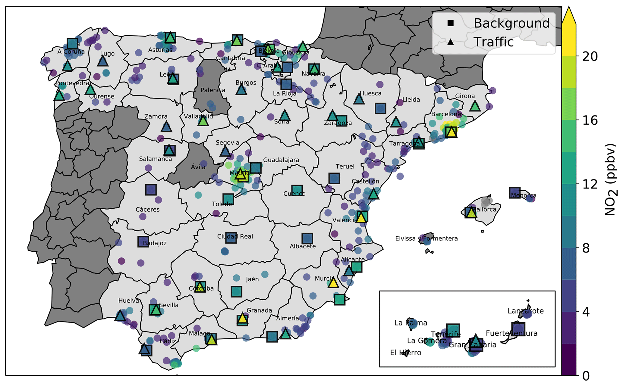
Figure 1Mean NO2 mixing ratios (ppbv; 2013–2020) at all (circles) and selected (squares and triangles) stations. Administrative borders show the NUTS-3 administrative units, which correspond to the Spanish provinces over the mainland and to individual islands. Dark gray areas indicate provinces and islands with a lack of stations that fulfill the selection criteria.
2.3 Methodology
We implement and train ML models to estimate the daily NO2 mixing ratios that would have been observed without the implementation of the lockdown in each selected station, i.e., under business-as-usual emission forcing. Hereafter, we will refer to these mixing ratios as business-as-usual NO2.
2.3.1 Machine-learning model
In this study, we retain the gradient boosting machine (GBM), a popular decision-tree-based ensemble method belonging to the boosting family (Friedman, 2001). More information on this model is given in Appendix B. ML models based on decision trees offer several interesting attributes. First, they internally handle the process of feature selection, which allows for the inclusion of potentially useless features without strong deterioration of the prediction skills. Second, they provide useful information about the importance of the different features. Third, in contrast to most parametric methods that derive a unique (more or less sophisticated) function supposedly valid over the whole features' space, nonparametric methods based on decision trees internally rely on successive splitting operations (a mother branch being divided into two daughter branches), which may be convenient for designing one single model that is able to work efficiently under different seasonal and weather regimes.
2.3.2 Choice of features and modeling strategy
Following the work of Grange and Carslaw (2019), the idea here is to use past recent data to train an ML model that is able to reproduce the NO2 mixing ratios based on a combination of meteorological features and other time features. The features used in this study are the daily mean 2 m temperature, minimum and maximum 2 m temperature, surface wind speed, normalized 10 m zonal and meridian wind speed components, surface pressure, total cloud cover, net solar radiation at the surface, downward solar radiation at the surface, downward UV radiation at the surface, boundary layer height, date index (days since 1 January 2013), Julian date and weekday. All of the data used in this study are daily. Some pollutant concentrations are known to strongly vary depending on the season and day of the week, notably due to the variability in emissions and chemistry. The two last time features act as proxies for these processes and aim to representing their climatological variations. Over longer (multi-annual) timescales, air pollutant concentrations cannot typically be considered as stationary due to substantial trends (especially in emissions), which is intrinsically problematic for training ML models. Following Grange et al. (2018) and Grange and Carslaw (2019), we introduced the date index as a proxy for this potential trend. Including such a feature with unique values (from 0 for 1 January 2013 to 2669 for 23 April 2020) is not expected to directly help the ML model to learn about NO2 variability; however, it allows us to train one single ML model over a relatively long and, thus, potentially nonstationary time series. In contrast to linear regression, GBM does not learn equations relating the target variable to the different features but rather builds nonparametric relationships between the target and features. As a consequence, such a model will always make NO2 predictions within the range of NO2 values used in the training, regardless of the inclusion of the aforementioned date index feature or the feature values it uses to make the predictions. However, if NO2 strongly increases (decreases) with time in the training dataset, the GBM model is able to split the data using the trend feature and, therefore, predict NO2 in the range of the higher (lower) mixing ratios reached by the end of the training period. We note that even with a trend feature, such a model is not expected to stay valid very far in time relative to the training data when the training data follow an overly strong trend. Our sensitivity tests have clearly shown that the behavior of the ML models substantially improves when including the trend feature.
In our study, the GBM models are trained and tuned over the 3 last full years, namely 2017–2019, and then used to predict business-as-usual NO2 mixing ratios over the 4 following months, from January to April 2020. This ML experiment is hereafter referred to as EXP2020. Such a duration for training is expected to allow for a substantial part of the interannual variability of NO2 mixing ratios and meteorological conditions to be captured and ensures some past data are available for quantifying the uncertainties of our ML modeling strategy (as explained later in Sect. 2.3.3). Note that no improvement was found with extended training periods of 4 or 5 years. Although our interest is to predict NO2 during the lockdown period, the 2.5 preceding months were kept to test the validity of our predictions and uncertainty estimates.
The machine-learning modeling in this study is performed using the “scikit-learn” Python package (Pedregosa et al., 2011). The GBM model comprises a number of hyperparameters to be tuned. Since features are temporal variables, instances cannot be considered as independent due to autocorrelation. Thus, we tuned our ML models using the so-called time series cross-validation with five splits, which corresponds to a rolling-origin cross-validation in which data used for the validation are always posterior to the data used for the training (“TimeSeriesSplit” in scikit-learn). Over a selection of the most important hyperparameters, we applied a so-called “randomized search” over a range of possible hyperparameter values. Compared with the so-called “grid search” in which all combinations of hyperparameters are tested, the randomized approach tests only a certain number (20 in our case) of tuning configurations that are chosen randomly. This allows for the exploration of a large part of the hyperparameters' space at a greatly reduced computational cost, and it tends to be less prone to overfitting. More details on the tuning of the GBM model can be found in Appendix C.
2.3.3 Uncertainty estimation
In order to quantify our prediction uncertainty, we replicated four similar experiments over the past years since 2013, i.e., training ML models over 2013–2015, 2014–2016, 2015–2017 and 2016–2018 and testing them over the 4 first months of 2016, 2017, 2018 and 2019, respectively. These ML experiments are hereafter referred to as EXP2016, EXP2017, EXP2018 and EXP2019, respectively. We obtained on average 538 daily residuals (predicted minus observed NO2 daily mixing ratios) for each station, and we took the associated 5th and 95th percentiles as the uncertainty interval for our ML-based predictions of daily NO2 mixing ratios. Therefore, for each station, we obtained a fixed asymmetric 90 % confidence interval used to characterize the uncertainty of our predictions during the first 4 months of 2020. Averaged over all Spanish provinces, the uncertainty interval is [−5.1, +5.3] ppbv at urban background stations and [−6.6, +6.7] ppbv at traffic stations.
In 2020, the period before the lockdown, namely 1 January to 13 March, is used to check the performance of the ML models trained over the period from 2017 to 2019 against the observed NO2 mixing ratios, given the aforementioned uncertainty. Ideally, we expect the differences between observed and predicted NO2 mixing ratios to remain within the estimated uncertainty during that period. Conversely, after 14 April, due to the reduction in NO2 emissions caused by the lockdown, we expect the observed NO2 mixing ratios to quickly decrease compared with the business-as-usual NO2 mixing ratios predicted by the ML model, eventually down to a level at which the differences are statistically significant.
These uncertainties are suited for our ML-based daily NO2 predictions. Because these daily uncertainties are likely at least partly uncorrelated, NO2 daily predictions averaged over time periods longer than 1 d are expected to have smaller uncertainties due to error compensations. We estimated the uncertainty affecting our ML predictions at the weekly scale. We used a similar approach to that previously described for the daily uncertainty but based on the 7 d running average of the daily residuals (by requiring a minimum of 5 over 7 d with available data). The 5th and 95th percentiles were computed based on the entire set of residuals (514 residuals on average at each station from 2016 to 2019). On average over all provinces, the weekly uncertainty intervals obtained are [−3.8, +3.6] ppbv at urban background stations and [−4.9, +4.7] ppbv at traffic stations, which represents a reduction of 28 % for both types of stations with respect to the daily uncertainties.
Our main interest in this study is to quantify the mean NO2 changes during the lockdown period. We decided to keep the weekly scale uncertainties for the predictions of business-as-usual NO2 mixing ratios averaged over its different phases (10–13 d each) and over the entire lockdown period (41 d). The use of weekly uncertainties is likely conservative when used for the entire lockdown average but accounts for potential data gaps, particularly when estimating the shorter phases therein.
Note that the ancillary ML experiments used here for quantifying the uncertainties also allow for the evaluation of the performance of our modeling strategy during the period of the year of the lockdown (as explained later in Sect. 3.1).
In this section, we first evaluate the ML-based predictions of business-as-usual NO2 mixing ratios (Sect. 3.1). We then illustrate our methodology in the two provinces with the largest population density, namely Madrid and Barcelona (Sect. 3.2). Time series for the other 48 Spanish provinces can be found in the Supplement. We then analyze the meteorology-normalized changes in NO2 obtained for all Spanish provinces (Sect. 3.3). In Sect. 3.4, we discuss the potential relationships with emission reductions. Finally, in Sect. 3.5, we discuss the advantages of our ML-based approach for estimating the baseline NO2 pollution compared with the climatological approach.
3.1 Evaluation of machine-learning predictions
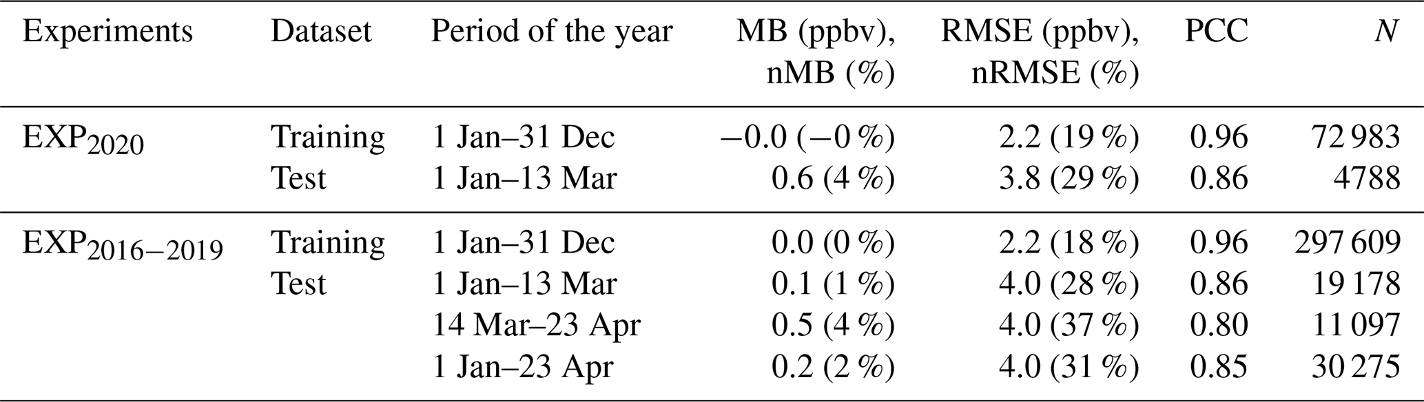
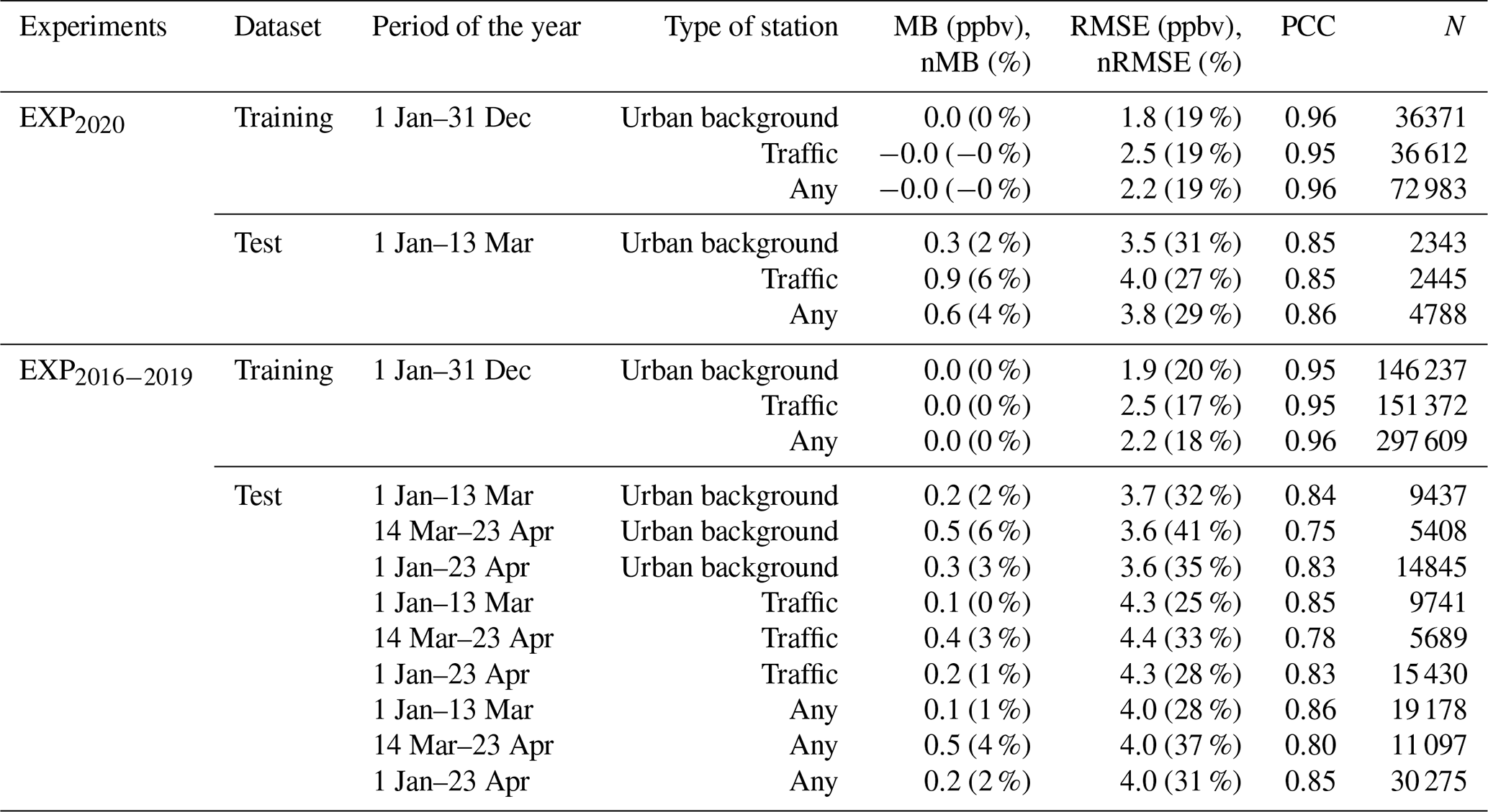
The performance of the ML predictions for each Spanish province and station type is shown in Fig. 2, and the statistics over all Spanish provinces are reported in Table 1. The statistical results in Table 1 are given for both the reference ML experiment (EXP2020) and the other experiments combined (EXP2016, EXP2017, EXP2018 and EXP2019, hereafter referred to as EXP2016−2019). Besides providing a broader view of the performance of our modeling strategy, considering these past experiments also allows for an assessment of the performance of the ML predictions during the period of the year of the lockdown (14 March–30 April for years 2016 to 2019), which may be important given the potential seasonality of prediction errors. The statistics obtained at urban background and traffic stations are given in Table C2 in the Appendix. Results are evaluated using the following metrics, which are calculated based on daily NO2 mixing ratios: mean bias (MB), normalized mean bias (nMB), root mean square error (RMSE), normalized root mean square error (nRMSE) and Pearson correlation coefficient (PCC).
For information purposes, we included the statistical results obtained over the training dataset (1 January 2017–31 December 2019 in EXP2020). Checking results over the training data may be useful for highlighting obvious situations of overfitting, when the performance is almost perfect. At both urban background and traffic stations, results show no bias, a low nRMSE (always below 35 %; 19 % when considering all provinces) and a high PCC of 0.96. Similar results are obtained when considering the ensemble of all past experiments (EXP2016−2019). Although such performance is very good, there are no clear signs of overly prejudicial overfitting at this stage.
On the test dataset of the EXP2020 reference experiment (1 January–13 March 2020, before the lockdown), the performance remains reasonably good in most provinces. Over all of the Spanish provinces, the nMB increases to +4 %, the nRMSE increases to 29 % and the PCC is reduced to 0.86, which is in very close agreement with the performance obtained with EXP2016−2020 (nMB of +1 %, nRMSE of 28 % and PCC of 0.86). In comparison, the performance obtained in EXP2016−2019 during the period of the year of the lockdown (14 March–23 April) is a bit lower but remains reasonable, with a nMB of +4 %, a nRMSE of 37 % and a PCC of 0.80. Although moderate, such a deterioration in performance after mid-March might reflect some seasonality in the ML model errors and/or could be related to the presence of trends in the NO2 concentrations. Concerning this last point, as previously discussed in Sect. 2.3.2, including the date index feature in the ML model aims to limit this potential issue but likely cannot completely solve it. Generally, only minor differences in performance are found between urban background and traffic stations (Table C2).
Results of EXP2020 per province (Fig. 2) highlight some interregional variability in the performance, with poorer statistics in some provinces, at least for one type of station. At most stations, the bias remains below ±20 % while the nRMSE ranges between 15 % and 45 % (highest nRMSE around 50 % in Teruel, Tenerife and Fuerteventura). Most provinces show a PCC of around 0.6–0.9, with only a few exceptions below 0.6 (urban background sites in Bizkaia, Fuerteventura and Huesca, and traffic sites in Granada and Gran Canaria).
Table 1 Performance of the ML predictions of NO2 mixing ratios. Results are shown for the reference experiment EXP2020 and for the ensemble of past experiments (EXP2016−2019).
Several factors may explain the poorer statistical results obtained at some stations. First and foremost, it may be due to deficiencies in the ML modeling, in particular to some overfitting. This seems to be the case for Fuerteventura and Huesca, given the good performance obtained with the training data (note also that the data availability of test data in Fuerteventura is among the poorest). Since we consider numerous stations in this study, we need a fixed procedure that can be applied similarly to all ML models to be trained. As described in Sect. 2.3.2, we designed our training and tuning procedure in order to limit this common issue as much as possible, using rolling-origin cross-validation and randomized search in the hyperparameters space. Overall the results are satisfactory, but some overfitting can still persist in some cases.
Second, although moderately, some of the biases and errors may be partly due to trends and/or interannual variability in NO2. As previously explained (Sect. 2.3.2), by model design, if the NO2 levels in the first months of 2020 are outside of the NO2 range in the 2017–2019 training dataset, our predictions over the lockdown period could be equally biased. The different NO2 time series indeed show some cases where NO2 mixing ratios are lower than in the past years (since 2013). In the framework of our study, it is important to mention that, although the lockdown was officially implemented on 14 March, COVID-19 started to perturb the business-as-usual situation in the days and weeks before – first through the cancellation of numerous events and, later, through unusual movements of a part of the population (e.g., to second homes). Although complicated to assess more precisely in each of the Spanish provinces, this likely explains part of the biases noticed in the second half of the test period.
Third, poor performance for some stations may be due to weaker relationships between meteorological input data and NO2 mixing ratios. This points to uncertainties in the ERA5 meteorology data. For example, the relatively coarse spatial resolution (31 km) of ERA5 data may only capture part of the meteorological variability existing at a given station. This is especially true when considering stations located in urban areas where the complex urban morphology (e.g., presence of buildings, canyon streets) is known to locally distort the mesoscale circulation. Decision-tree-based ML methods like GBM offer some interpretability by providing a measure of the importance of the different features included as input data. In our case, on average over all ML models, the most important feature is the boundary layer height (18±6 %) followed by the surface wind speed (12±5 %). These two parameters drive the ventilation and dispersion of the pollutants emitted at the surface, and their variability at some stations may be only partly captured by the ERA5 data at some urban stations. Also, the ERA5 data may poorly capture the meteorological conditions at some stations located on small islands with complex orography, like in the Canary Islands (e.g., Tenerife and Fuerteventura).
The chosen training and tuning procedures applied in this study were designed to limit some of these different sources of uncertainty, but persistent errors cannot be excluded. This is why we added another layer of analysis in which we estimated the uncertainties of our ML predictions by replicating exactly the same procedure over the past years since 2013 (as explained in Sect. 2.3.3). Computed as the 5th and 95th percentiles of the daily residuals obtained over a large test period extending over several years (2016–2019), the uncertainty intervals are expected to cover most (90 %) of the errors caused by these different sources of uncertainties. Indeed, considering all stations, our results indicate that 89 % (4240 points over 4788) of the daily NO2 observations in 2020 before the lockdown fall within the corresponding prediction uncertainty interval at each station, which is very close to 90 %. This demonstrates that the daily uncertainty estimated in this study is well quantified.
All in all, we have shown that our ML predictions and associated uncertainties are qualified for estimating the business-as-usual NO2 mixing ratios during the lockdown.

Figure 2Statistical results of the ML-predicted business-as-usual NO2 mixing ratios (EXP2020 reference experiment) over the training dataset (2017–2019, in gray) and test dataset before lockdown (1 January–13 March 2020, in blue). Metrics are mean bias (MB), normalized mean bias (nMB), root mean square error (RMSE), normalized root mean square error (nRMSE) and Pearson correlation coefficient (PCC). For information purposes, the uncertainties (90 % confidence interval) at the daily scale are added to the MB (horizontal blue bars).
3.2 Illustration of the results in specific provinces
3.2.1 Madrid
The daily NO2 mixing ratios observed and predicted in the province of Madrid are shown in Fig. 3 for both the urban background station and the traffic station, with station codes (names) ES1941A (Ensanche de Vallecas) and ES1938A (Castellana), respectively. The NO2 mixing ratios observed over the past years since 2013 are also included. Since days of the week are not consistent from one year to another, we also show the NO2 7 d running mean time series where a minimum of 5 over 7 d is required to compute the average.
In Madrid, the ML reproduces the variability in NO2 mixing ratios at the urban background and traffic stations before the lockdown remarkably well (nMB of −3 and +6 %, nRMSE of 19 % and 22 %, PCC of 0.87 and 0.85, respectively). Importantly, prediction errors remain within the uncertainty interval. The two subperiods with lower NO2 mixing ratios, during the second half of January and early March, occur concomitantly with strong wind speeds in Madrid, above 6 m s−1 on a daily average (above the 95th percentile of the ERA5 daily wind speed from 2013 to 2020 during this season), and relatively high boundary layer heights (up to 1000–1500 m on a daily average). It is worth mentioning that a low emission zone (LEZ) with relatively strict vehicle restrictions applied for entering a limited area of about 5 km2, corresponding to the heart of the city center, was implemented in early January 2020. Such a change in emissions may, in principle, directly impact the performance of the ML predictions by inducing a positive bias (as the ML models are designed precisely for highlighting such events). In our case, we expect a limited impact because the LEZ was still in its transition phase (strict enforcement via fines for offending motorists was not expected until 1 April and was finally postponed until 15 September 2020 due to the COVID-19 situation) and the two stations selected in Madrid province are located outside of the LEZ (9 and 3 km from the city center, respectively).
After the implementation of the lockdown, the observed NO2 mixing ratios decreased down to about 11 and 7 ppbv on average, and they reached daily minimum mixing ratios of 6 and 3 ppbv, respectively, over the entire period. Compared with the previous years, the NO2 mixing ratios at the urban background site are clearly in the lower tail of the distribution. At the traffic site, NO2 levels had not been that low for such an extended period of time since at least 2013. In comparison, business-as-usual NO2 mixing ratios at these two sites would have remained at around 17–18 ppbv on average. After the lockdown, the differences between the observed and business-as-usual NO2 are found to progressively increase, becoming more and more statistically significant. This demonstrates unambiguously that the lockdown considerably reduced the NO2 pollution in Madrid, regardless of the meteorological conditions, which points to a drastic decrease in the business-as-usual emission forcing.
We computed the meteorology-normalized change in NO2 during the lockdown period covered by this study (from 14 March to 23 April) as the mean difference between ML-based business-as-usual and observed NO2 daily mixing ratios. The uncertainty at the weekly scale is used here as an estimate of the uncertainty at a 90 % confidence level (by construction, given that they are computed as the 5th and 95th percentiles of the weekly residuals, see Sect. 2.3.3) affecting the mean NO2 change. On average over the entire lockdown period, NO2 levels have decreased by ppbv at the urban background station, which corresponds to % in relative terms. The impact is faster, stronger and more statistically significant at the traffic station than at the urban background site, with a mean NO2 reduction of ppbv, or % in relative terms. This result is consistent with a lockdown most strongly affecting the traffic emissions sector. At the daily scale, the reduction in NO2 in Madrid reached its maximum at the end of the second and more stringent lockdown phase, while a strong reduction persisted during the third phase.
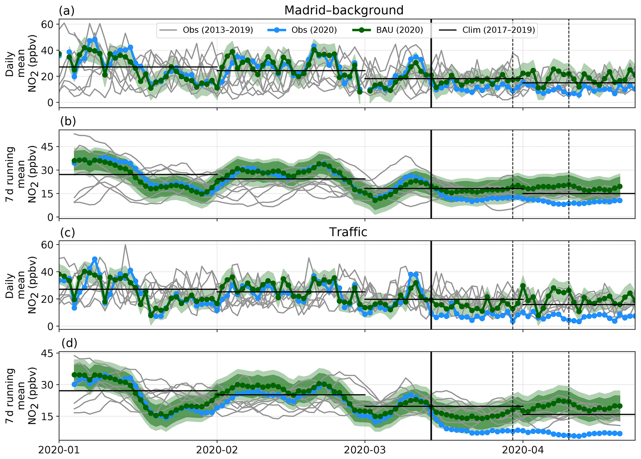
Figure 3NO2 mixing ratios in Madrid province. Panels (a) and (b) show the daily mean and the 7 d running mean at the urban background station, respectively. Panels (c) and (d) show the time series at the traffic station. Each panel displays the NO2 mixing ratios observed in 2020 (in blue) and during the past years (2013–2019, in gray), and the NO2 mixing ratios predicted in 2020 by the ML model (business-as-usual – BAU, in green). The uncertainties of the ML predictions are given at a 90 % confidence level at the daily (light green) and weekly scales (medium green). The climatological monthly averages computed over the period from 2017 to 2019 are also shown (in black). The vertical black line identifies the beginning of the lockdown, and the next dotted lines separate the different lockdown phases (phase I: 14–29 March 2020; phase II: 30 March–9 April 2020; phase III: 10–23 April 2020).
3.2.2 Barcelona
Figure 4 presents the results for Barcelona for both the urban background and traffic stations, with station codes (names) ES1396A (Sants) and ES1480A (L'Eixample), respectively. Compared with Madrid, the ML predictions in Barcelona have relatively similar errors (nRMSE of 25 %) and correlations (PCC of 0.72). The bias is very low at the urban background station (+0 %), and it reaches +8 % at the traffic station, which largely remains within the uncertainty interval. The positive bias in the traffic station started in early February and persisted during the following weeks, particularly after the second week of February. The ML model failed to reproduce these low NO2 mixing ratios, notably because some of the observed NO2 mixing ratios during that period were lower than during the previous years. As in Madrid, a LEZ was implemented in Barcelona, starting in early January 2020, with less stringent vehicle restrictions but over a larger area (95 km2). Both the urban background and traffic stations selected in Barcelona are included in this LEZ. The potentially stronger effect of the LEZ on traffic stations could at least partly explain this positive bias. As in the case of Madrid, fines for noncompliance with the LEZ restrictions were not planned to start before 1 April (postponed to 15 September 2020 due to the COVID-19 situation). Therefore the effect of the LEZ is expected to be progressive, which is consistent with the absence of a bias at the beginning of the period. In addition, the 2020 World Mobile Congress (the largest annual event in Barcelona, with 109 000 visitors in 2019) that takes place every year by the end of February was officially canceled by the organizers due to the risks posed by the emerging COVID-19 pandemic. Therefore, we hypothesize that this cancellation contributed to the reduction in NO2 levels in the city and to the slight positive bias of the ML prediction before the lockdown.
After the lockdown, NO2 mixing ratios decreased down to 8 and 11 ppbv on average at the urban background and traffic stations, respectively, both reaching minimum daily mixing ratios of 4 ppbv. These results highlight strong and statistically significant differences with the business-as-usual situation in which NO2 levels would have remained at around 15–21 ppbv during that period. As in Madrid, the strongest differences are found in April, during phases II and III of the lockdown. Note that these differences greatly exceed the aforementioned positive bias encountered after February. Interestingly, besides the strong reduction, observed NO2 mixing ratios followed a very similar variability to business-as-usual NO2, which highlights the major influence of meteorological conditions on the levels of pollution, as previously mentioned by Tobías et al. (2020). For instance, the increase in NO2 mixing ratios between 6 and 9 April appears linked to unusually low wind speeds over Barcelona (1.7 m s−1 on average over these days), which is slightly below the climatological (2013–2020) 5th percentile of wind speed in April (1.8 m s−1). Without the lockdown, this stagnant situation associated with the business-as-usual emission forcing would have increased NO2 by about 5–10 ppbv, according to the ML predictions. Observed NO2 also slightly increased during the episode of stagnant meteorological conditions, but due to the lockdown, NO2 remained at very low levels. This event illustrates the usefulness of considering an ML model fed by meteorological data for quantifying the baseline air pollution during the lockdown.
Over the entire lockdown period, NO2 in Barcelona decreased by ppbv ( %) at the urban background station, regardless of the meteorological conditions. As in Madrid, a stronger reduction is found at the traffic station, with ppbv ( %). Therefore, in relative terms, the lockdown induced a relatively similar decrease in NO2 in both Madrid and Barcelona.

3.3 Meteorology-normalized changes in NO2 mixing ratios over Spain
We computed the meteorology-normalized changes in NO2 for all of the selected stations. The results are presented in Fig. 5, along with the weekly uncertainty of our ML predictions (colored lines). For information purposes, we also display the daily uncertainty (black lines). Results are colored as a function of their degree of significance, here computed as the distance between the NO2 change best estimate and the upper limit of the weekly uncertainty interval, normalized by the distance between the best estimate and zero. Thus, a degree of significance of 1 indicates an NO2 change significant at a 90 % confidence level. Statistics regarding the changes in NO2 obtained in all provinces are reported in Table 2. A map of best estimates of NO2 changes at each station is also given in Fig. 6.
Results highlight that the reduction previously described in Madrid and Barcelona extends to most Spanish provinces, although with some interregional variability in the extent of the change and the degree of statistical significance. During the lockdown period, 96 % (2734 points over 2844) of the observed daily NO2 mixing ratios are lower than the ML-based business-as-usual NO2 estimates. On average over all urban background stations during the entire lockdown period, NO2 has decreased by ppbv (] % in relative terms), independently of the meteorological conditions. The 5th and 95th percentiles (computed based on the mean NO2 changes obtained in all provinces) are −7 ppbv (−65 %) and −1 ppbv (−31 %). The NO2 change is significant with more than 90 % confidence in 22 out of 38 provinces, with many of the remaining sites being relatively close to that confidence level. A similar yet more statistically significant reduction is found at traffic stations, with a mean NO2 decrease of ppbv (or %) and 26 out of 37 stations exceeding the 90 % confidence level. The spread of NO2 change between the different provinces is also quite similar between the two types of stations, with 5th and 95th percentiles of −69 % and −29 %, respectively. Generally, the meteorology-normalized NO2 reductions in the provinces of the southern half of the country appear stronger and in more cases statistically significant.
As previously observed in Madrid and Barcelona, the results in Table 2 highlight noticeable differences between the different phases of the lockdown. The corresponding figures (with both absolute and relative changes) can be found in the Appendix (Figs. C1, C2, C3 and C4). The mean reduction in NO2 during phase I was about −42 % at both station types, and it further increased to about −54 % during phases II and III. The lower reduction during the first phase is partly explained by the fact that NO2 concentrations started at their business-as-usual levels and took a few days to reach their minimum. During the two last phases, NO2 was found to be reduced in many more provinces, as shown by the 95th percentile that ranges between −20 and −40 % depending on the type of station during phases II and III, compared with only −9 % to −19 % during phase I.

Figure 5Meteorology-normalized mean NO2 changes at urban background (squares) and traffic (triangles) stations during the COVID-19 lockdown. Changes are shown during the entire lockdown period and during the second and most stringent phase. Best estimates and weekly uncertainties are colored according to the degree of significance (a value of 1 indicates a change that is statistically significant at a 90 % confidence level, see text for more details). For information purposes, daily uncertainties are also indicated (black lines). For comparison, the mean NO2 changes obtained using the climatological average (from 2017 to 2019) rather than the ML-based business-as-usual NO2 concentration are also shown (stars), as well as the relative difference between both approaches (circles).
Table 2 Meteorology-normalized changes in NO2 mixing ratios in Spain during the lockdown (phase I: 14–29 March 2020, phase II: 30 March–9 April 2020, phase III: 10–23 April 2020). Statistics are computed based on the mean NO2 changes in the different Spanish provinces.
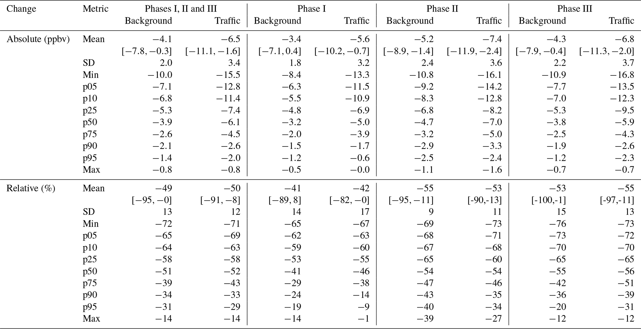
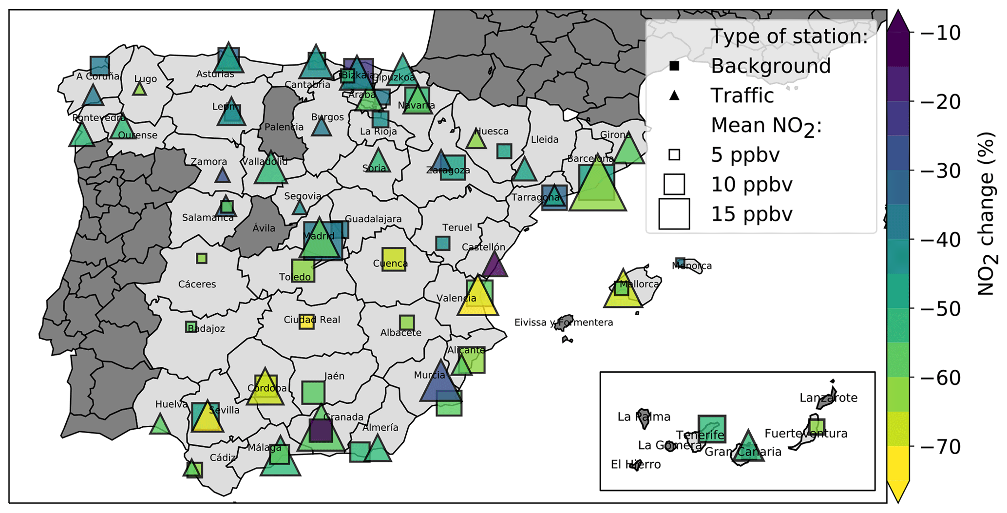
Figure 6Meteorology-normalized mean NO2 changes at selected urban background and traffic stations during the COVID-19 lockdown in Spain. The size of symbols is proportional to the annual average NO2 mixing ratio (from 2013 to 2020).
3.4 Relationship to emission reductions
We contrasted our results with a detailed NOx anthropogenic emission inventory at 4 km×4 km resolution over Spain available through the bottom-up module of the HERMESv3 emission model, developed at the Earth Sciences Department of the Barcelona Supercomputing Center (Guevara et al., 2020b). Averaged over the different stations considered in this study, road transport emissions are the dominant source, with 66 and 69 % of the total NOx emissions in the vicinity of urban background and traffic stations, respectively. The other emission sources are the residential and commercial combustion sector (14 % and 15 %), industrial point sources (8 % and 13 %), and shipping and port activities (11 % and 3 %). In Spain, the public agency in charge of monitoring traffic (Dirección General del Tráfico) reported progressive reductions in total traffic down to levels about −60 % to −90 % lower than usual, with substantial day-to-day variability and strongest reductions during weekends. Assuming to first order a linear relationship between NO2 urban background mixing ratios and local surrounding NOx emissions (within a 4 km×4 km cell) and applying a 70 % (80 %) reduction in road transport would lead to a NO2 reduction of about 47 % (54 %), which is consistent with our findings. Our knowledge about the impact of the lockdown on the other emission sectors remains quite limited at this stage. NOx emissions from industry likely also decreased but quantifying this reduction, even roughly, is more complex as some industries were considered to be essential and, thus, were not affected by the lockdown. Although 9 %–13 % of the surrounding emissions (in the 4 km×4 km cell of the inventory) are associated with this sector, the impact of idling industrial activities on the pollution levels observed at the selected stations may be relatively small considering that none of these stations are classified as “industrial”. The residential and commercial emission sector represents another unknown, as the expected emission increment caused by a population spending more time at home may be compensated for by the closure of most shops, schools and offices. A more detailed analysis of the activity data in these different emission sectors is required to better quantify how the emission forcing has been modified by the lockdown (Guevara et al., 2020a) and to understand the reductions in NO2 obtained in this study.
Concerning traffic stations, although HERMESv3 gives a quite similar contribution of the different emission sectors compared to urban background stations, a larger contribution of road transport emissions is evidently expected as measurement instruments are deployed under the direct influence of vehicles. As a consequence, assuming that road transport is the emission sector most impacted by the lockdown (along with air traffic, although this last sector does not emit strong amounts of NOx around our set of stations), we could expect a stronger relative reduction in NO2 at traffic stations, compared with urban background stations. At first glance, Table 2 does not highlight such a difference between the two types of stations. This seems to be due to the fact that we gather urban background and traffic stations that are not always co-located in the same cities and/or that are located in cities of very different sizes. In both Madrid and Barcelona provinces, the two selected stations are located in the same agglomeration, and the results do highlight substantial differences in NO2 reductions (Sect. 3.2). In total, urban background and traffic stations are co-located in the same agglomeration in 16 provinces. On average over this set of provinces, the NO2 reduction is −44 % and −53 % at the urban background and traffic stations, respectively, showing a noticeable but still relatively small difference. Focusing on the six largest cities within this group of provinces (Madrid, Barcelona, Valencia, Sevilla, Málaga and Mallorca), the difference in NO2 reductions increases, with −50 % and −63 % at urban background and traffic stations, respectively. Focusing on the two largest cities, namely Madrid and Barcelona, the discrepancy further increases, with NO2 reductions of −43 % and −60 %, respectively. Therefore, results suggest that the lockdown has more strongly impacted the business-as-usual NO2 levels at traffic stations than those at urban background sites and that this difference tends to be stronger in the largest cities.
3.5 Machine-learning-based business-as-usual NO2 versus climatological average NO2
We developed the ML-based approach arguing that it allows for avoiding potentially erroneous assessment of the lockdown-related NO2 changes caused by the variability of meteorological conditions. In this section, we quantitatively illustrate the benefits of our method. Besides the business-as-usual NO2 daily concentrations obtained with our ML-based approach, we consider the mean NO2 concentrations observed in the period from 2017 to 2019 during the time of the year in which the lockdown took place (this approach hereafter being referred to as the climatological average approach). We compared the mean NO2 concentrations obtained in each province with both approaches during the different phases of the lockdown. Taking the ML-based approach as a reference, we computed the bias of the climatological average approach. In this frame, in a given province, a small bias between the two approaches should indicate that the meteorological conditions prevailing during a given phase of the lockdown are relatively close to their climatological values at this time of the year. For convenience, both urban background and traffic stations are gathered in this analysis.
The NO2 changes obtained with the climatological average approach are reported in Fig. 5 (and for the different phases in Figs. C1, C2, C3, C4 in the Appendix). Considering the entire lockdown period, the mean business-as-usual NO2 mixing ratio predicted by the ML models averaged over all provinces is 10.3 ppbv, which is in close agreement with the corresponding climatological mean NO2 of 10.6 ppbv. This corresponds to a mean bias (of the climatological average approach) of only +0.3 ppbv (or +2 % in relative terms). This shows that under a business-as-usual scenario, the NO2 concentrations during the lockdown period should have been close to the values typically observed at this time of the year. However, this holds at a relatively large temporal (the entire lockdown period in this case, i.e., 41 d) and spatial (all Spanish provinces) scale. These relative biases between both approaches are shown for all stations in Fig. 5 (black circles). Among the different provinces, they range between −41 and +33 %, with 5th and 95th percentiles of −22 and +27 %, which is greatly larger than its average of +2 %. This highlights the presence of substantial departures from the climatology at the province scale. For instance, in Barcelona province, the ML-based business-as-usual and climatological mean urban background NO2 mixing ratios during the lockdown period are 15 and 19 ppbv, respectively, which corresponds to a climatological approach that is positively biased by +27 %. Such a result is not surprising, as encountering the same climatological conditions simultaneously in all Spanish provinces is very unlikely.
Although it is higher when considered at the province scale, the bias of the climatological average approach can also further increase when computed over shorter time periods. Indeed, during the three phases of the lockdown, it reaches +12 %, +2.3 % and +1.8 %, respectively, when averaged over all provinces. Among the different provinces, the corresponding 5th and 95th percentiles reach −21 and +52 %, −34 and +44 %, and −41 and +36 % during phases I, II and III, respectively. For the case of Barcelona province, these relative biases are +35 %, +19 % and 22 % for the three respective phases of the lockdown.
This analysis demonstrates the need to take the meteorological variability into account (with ML or other techniques) in order to accurately estimate the baseline pollution and assess the changes in pollution induced by an altered emission forcing, which appears all the more crucial when pollution changes are investigated at a fine temporal and/or spatial scale.
The fast spread of the COVID-19 coronavirus disease pushed Spanish authorities to implement a severe lockdown of the population, with drastic restrictions of social and economic activities starting on 14 March 2020. This situation had an impact on the anthropogenic emissions from numerous activity sectors, some of them unambiguously (road transport and air traffic, and to a lesser extent the industrial sector) and others with a still unclear response (residential and commercial sector). Concomitantly, a reduction in NO2 mixing ratios was reported in many locations based on in situ NO2 measurements operated by air quality monitoring stations or space-based remote sensing (e.g., TROPOMI). Part of the reduction in NO2 pollution is likely explained by the modified emission forcing caused by the lockdown. However, the potential confounding impact of the meteorological variability (a major driver of the NO2 variability) prevents one from directly relating the reduction in NO2 mixing ratios to the lockdown-related reduction in emissions.
To tackle this issue, we used ML models fed by meteorological data and time variables (Julian date, day of week and date index) to estimate the NO2 mixing ratios that would have been normally observed during the COVID-19 lockdown period under a business-as-usual emission forcing and meteorological conditions prevailing during that period. We also estimated (conservative) uncertainties affecting our ML predictions. This allowed us to quantify the changes in NO2 during the lockdown that are not directly related to the variability of meteorological conditions. On average over Spain, NO2 mixing ratios at urban background and traffic stations were found to decrease by about −50 % due to the lockdown, with stronger reductions in phases II and III (about −55 %) than in phase I (about −40 %). We also demonstrated the benefits of our meteorology-normalized approach compared with a simple climatological-based approach, especially at smaller temporal and spatial scales.
Due to the peculiarities of NO2 (e.g., primary pollutant, short chemical lifetime and simple chemistry), we expect these changes to be mainly driven by the reduction in NOx anthropogenic emissions. Considering that the lockdown also impacted the emissions of numerous other chemical compounds, an alteration of the business-as-usual chemical fate of NO2 (via a modification of its oxidation into nitric acid) cannot be excluded. However, here we consider urban stations located close to the NOx emission sources, where this effect is likely small compared with the reduction in direct emissions.
Regarding our methodology, we note that the COVID-19 lockdown and the associated changes in pollutants, such as particulate matter, should have also altered the meteorological conditions by perturbing the radiative fluxes and clouds. Indeed, this methodology precludes the remote and local influences of lockdown-related air pollution changes upon local weather. In any case, given the chaotic nature of the atmosphere and the long duration of the lockdown, it would indeed be impossible to know the weather conditions that would had been observed during the lockdown in a business-as-usual scenario.
It is also worth noting that the quality of the ERA5 meteorological data may have deteriorated during the lockdown due to the strong reduction in air traffic. Indeed, although satellites remain the dominant provider of meteorological observations, commercial aircraft provide valuable amounts of in situ meteorological observations in the troposphere and lower stratosphere, especially regarding wind speed. However, some meteorological services are currently operating additional atmospheric soundings to compensate for this loss of data. In any case, the impact on the meteorological conditions close to the surface is probably limited.
In this work, we analyzed the NO2 data available in Spain over the first 41 d of lockdown, which includes the phase of most stringent lockdown in early April. At the date of submission of this study, the lockdown was still on-going in Spain, with restrictions planned to be progressively relaxed until late June at least. Indeed, the impact of the lockdown upon air pollution levels will likely extend far beyond the period considered in this study. Besides the direct effects of the lockdown-related restrictions, the foreseen economic downturn – the size, length and characteristics of which are still uncertain – may also substantially affect the levels of NO2 pollution, as has already observed following the 2008–2009 economic recession, with 1-year recession-driven NO2 reductions of 10 %–30 % across Spain and Europe (Castellanos and Boersma, 2012).
The results of the present study provide a valuable reference for validating similar assessments of the impact of the COVID-19 lockdown on air quality based on chemistry transport models and emission scenarios derived from activity data during the lockdown (e.g., Guevara et al., 2020a; Menut et al., 2020).
In a separate study, our meteorology-normalized estimates are used to quantify the circumstantial reduction in the mortality attributable to the short-term effects of NO2 during the lockdown (Achebak et al., 2020).
Using the information provided by GHOST (Globally Harmonised Observational Surface Treatment; Bowdalo, 2020), we applied numerous QA screening flags to the NO2 dataset, in order to remove the following: missing measurements (flag 0), infinite values (flag 1), negative measurements (flag 2), zero measurements (flag 4), measurements associated with data quality flags given by the data provider which have been decreed by the GHOST project architects to suggest that the measurements are associated with substantial uncertainty or bias (flag 6), measurements for which no valid data remain to average in the temporal window after screening by key QA flags (flag 8), measurements showing persistently recurring values (rolling seven out of nine data points; flag 10), concentrations greater than a scientifically feasible limit (above 5000 ppbv; flag 12), measurements detected as distributional outliers using adjusted boxplot analysis (flag 13), measurements manually flagged as too extreme (flag 14), data with an overly coarse reported measurement resolution (above 1.0 ppbv; flag 17), data with an overly coarse empirically derived measurement resolution (above 1.0 ppbv; flag 18), measurements below the reported lower limit of detection (flag 22), measurements above the reported upper limit of detection (flag 25), measurements with inappropriate primary sampling for preparing NO2 for subsequent measurement (flag 40), measurements with inappropriate sample preparation for preparing NO2 for subsequent measurement (flag 41) and measurements with erroneous measurement methodology (flag 42).
Among the myriad of ML models available nowadays, we opted for decision-tree-based ensemble methods. The general idea of ensemble methods is to combine an ensemble of independent base learners (or weak learners). Base learners here designate simple models that perform only slightly better than a random guessing. Decision trees are currently the base learner most commonly used in ML ensemble methods (but other types of learners could be possible). Given a training dataset and a regression problem, one characteristic of decision trees lies in the fact that it is always possible to reach a high accuracy (by growing a large enough tree) but at the cost of very poor generalization skills. In ML terminology, such large trees are said to have a small bias but a large variance. Thus, to be appropriate base learners, decision trees used in ensemble methods are constrained to have a low number of branches (sometimes referred to as trunks), which increases the bias but reduces the variance. The strength of ensemble methods then stems from the fact that combining a sufficiently large number of base learners (of quite poor performance individually) allows one to obtain enhanced performance in addition to better generalization skills, with the corresponding ensemble being less unstable to the addition of new data.
Once the form of the base learner is chosen, a strategy is required for building this ensemble of “independent” base learners. Three main approaches have been proposed in the past: (i) bagging, (ii) boosting and (iii) random forests (RF). Bagging consists of aggregating base learners trained on a bootstrap sample of the training dataset. Boosting consists of aggregating base learners trained on different labels: the first base learner is trained on the dataset, the second is trained on the errors left by the previous one, the third on the errors left by the two previous ones and so on. RF, used by Grange et al. (2018) and Grange and Carslaw (2019), consists of aggregating base learners trained on random subsets of the training dataset based on a random subset of features.
The training of the model is conducted along with a search of the optimal hyperparameter tuning. We retained a so-called randomized search in which a range of values is given for each hyperparameter of interest and a total number of hyperparameter combinations to test (20 in our case). Compared with the so-called grid search in which all combinations of hyperparameters are tested; this choice allows for the exploration of a large part of the hyperparameters space for a greatly reduced computational cost, and it is less prone to overfitting.
We used the scikit-learn Python package. The learning rate was fixed to 0.05, and the number of features to consider when looking for the best split was fixed to the square root of the number of features (“max_features” in scikit-learn, set to “sqrt”). In addition, the tuning of the GBM model was done over the following set of hyperparameters: the tree maximum depth (“max_depth” in the scikit-learn Python package: values from 1 to 5 by 1), the subsample (“subsample”: values from 0.3 to 1.0 by 0.1), the number of trees (“n_estimators”: values from 50 to 1000 by 50) and the minimum sample in terminal leaves (“min_samples_leaf”: values from 1 to 30). The maximum depth (or the maximum number of subsequent splits in the individual decision trees) controls how much interaction between the features can be taken into account. The subsample hyperparameter represents the fraction of samples to be used for fitting an individual base learner. Values below unity correspond to the so-called “stochastic gradient boosting” and usually allow for a decrease in the variance at the cost of an increased bias (low values also allow for the training phase to be sped up). The minimum sample leaf hyperparameter controls the minimum number of samples that are allowed in a terminal node (larger values limit the risk of overfitting).
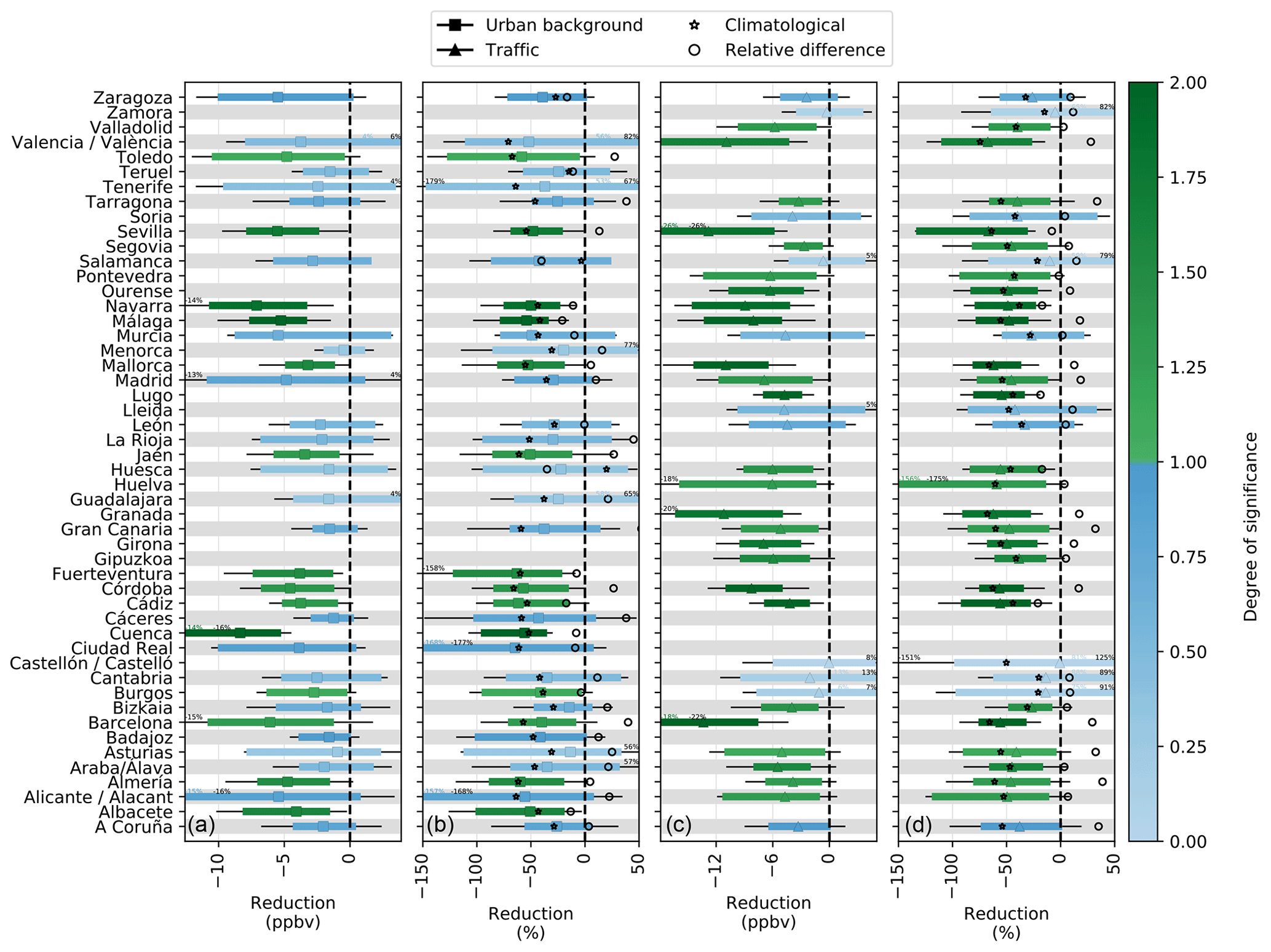
Figure C1Absolute and relative meteorology-normalized NO2 changes during phase I of the lockdown (14–29 March 2020) at urban background (a, b) and traffic stations (c, d). The uncertainties shown with colored bars correspond to the 90 % confidence level interval computed at the weekly scale. For information purposes, the uncertainties affecting the ML-based daily predictions are also shown (black bars). For comparison, the mean NO2 changes obtained using the climatological average (from 2017 to 2019) rather than ML-based business-as-usual NO2 concentration are also shown (stars), as well as the relative difference between both approaches (circles).
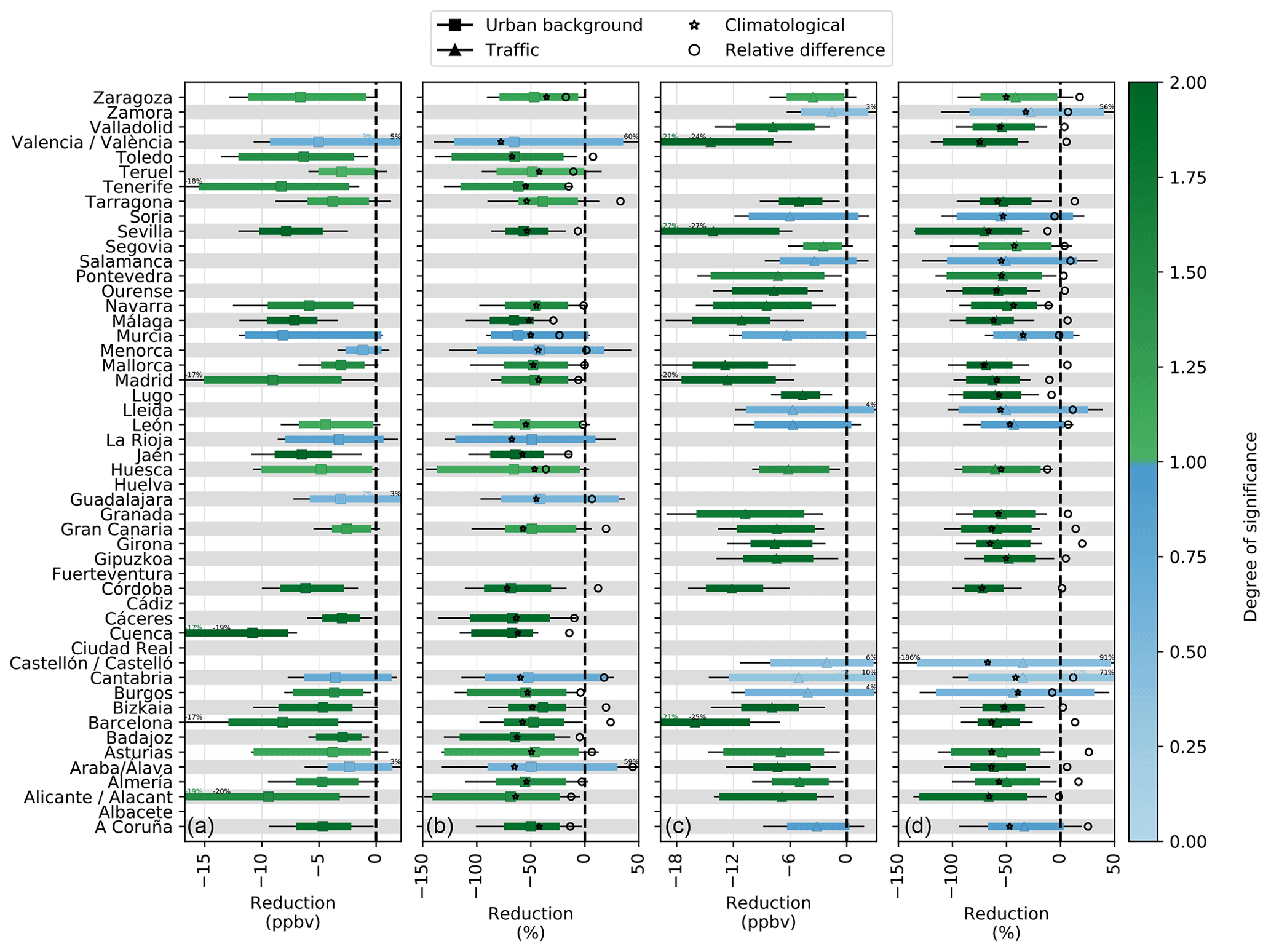
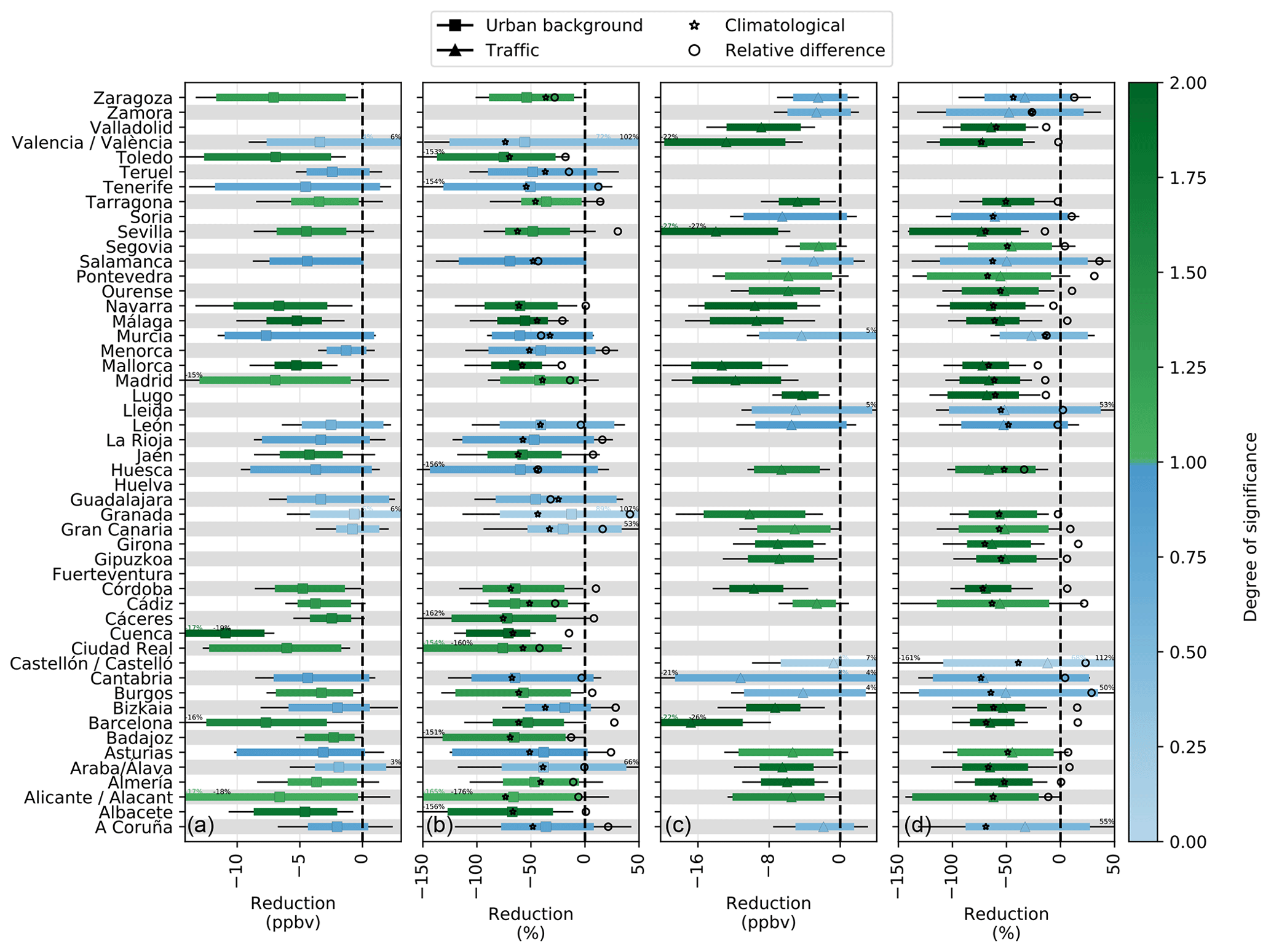
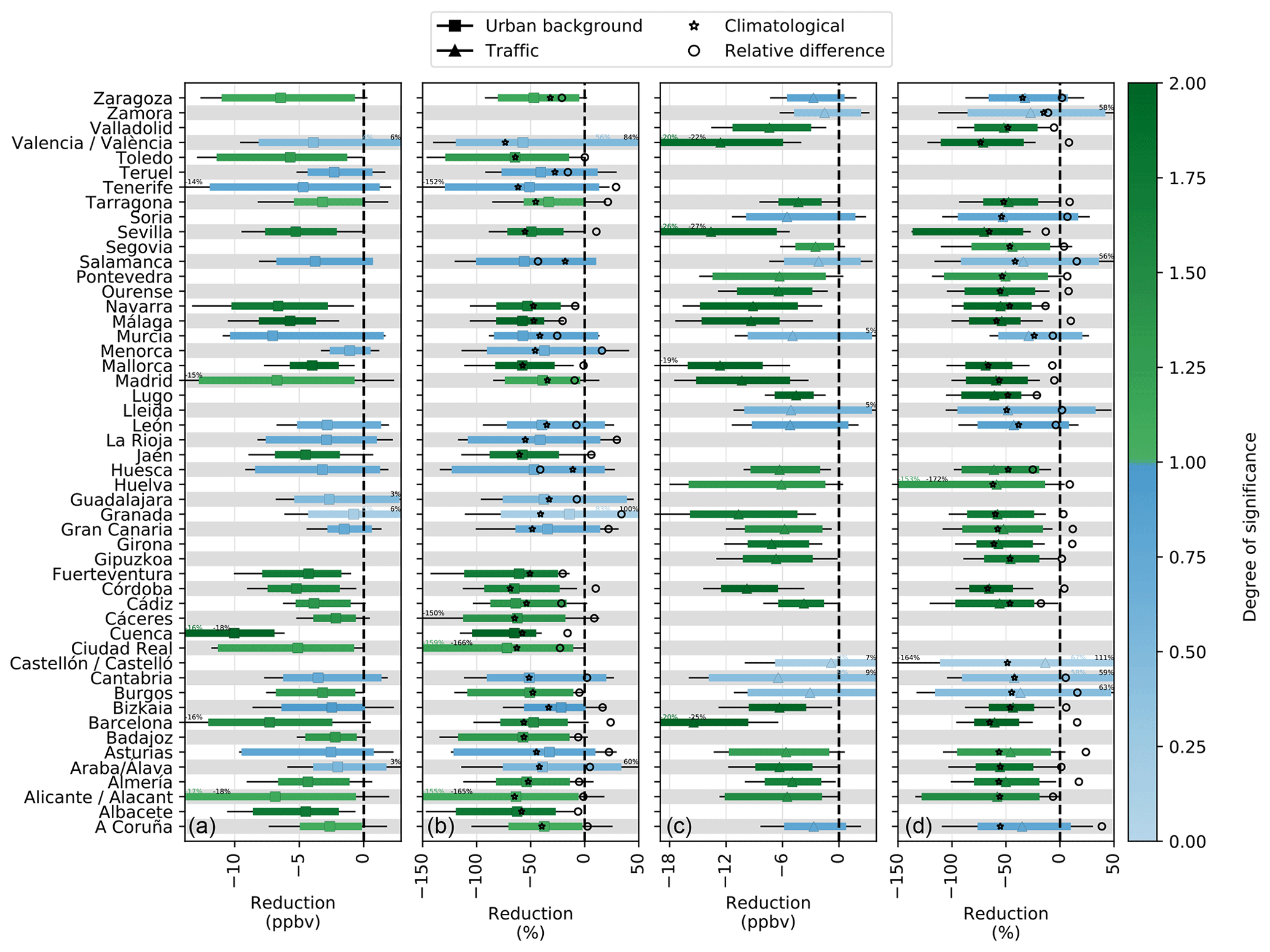

Table C2 Performance of the ML predictions of NO2 mixing ratios. Results are shown for both the reference experiment EXP2020 and for the ensemble of past experiments (EXP2016−2019).
The EEA AQ e-Reporting, ERA5 and Gridded Population of the World (GPW; version 5) datasets used in this study are publicly available. The HERMESv3_BU (bottom-up) code package with its documentation is publicly available at the following GitLab repository: https://earth.bsc.es/gitlab/es/hermesv3_bu (last access: 20 April 2020) (https://doi.org/10.5281/zenodo.3521897, Guevara et al., 2019).
The supplement related to this article is available online at: https://doi.org/10.5194/acp-20-11119-2020-supplement.
HP and CPGP contributed to the conception and design of the study. DB and KS were responsible for the acquisition of data. HP, DB, CPGP, MG, AS and OJ carried out the analysis and interpretation of data. HP and CPGP were responsible for writing the article.
The authors declare that they have no conflict of interest.
This project has received funding from the European Union's Horizon 2020 (H2020) research and innovation program under the Marie Skłodowska-Curie Actions (grant no. H2020-MSCA-COFUND-2016-754433) and the H2020 ACTRIS IMP project (grant no. 871115). We also acknowledge support from the European Research Council (grant no. 773051; FRAGMENT); the AXA Research Fund; the Spanish Ministry of Science, Innovation and Universities (grant nos. RYC-2015-18690, CGL2017-88911-R, RTI2018-099894-B-I00 and Red Temática ACTRIS España CGL2017-90884-REDT); and the BSC-CNS “Centro de Excelencia Severo Ochoa 2015-2019” program (grant no. SEV-2015-0493). The authors are grateful to PRACE for awarding us access to MareNostrum Supercomputer in the Barcelona Supercomputing Center.
This research has been supported by the H2020 Marie Skłodowska-Curie Actions (grant no. STARS 754433).
This paper was edited by Stelios Kazadzis and reviewed by two anonymous referees.
Achebak, H., Petetin, H., Quijal-Zamorano, M., Bowdalo, D., García-Pando, C. P., and Ballester, J.: Reduction in air pollution and attributable mortality due to COVID-19 lockdown, The Lancet Planetary Health, 4, e268, https://doi.org/10.1016/S2542-5196(20)30148-0, 2020. a
Anderson, R. M., Heesterbeek, H., Klinkenberg, D., and Hollingsworth, T. D.: How will country-based mitigation measures influence the course of the COVID-19 epidemic?, The Lancet, 395, 931–934, https://doi.org/10.1016/S0140-6736(20)30567-5, 2020. a
Bauwens, M., Compernolle, S., Stavrakou, T., Müller, J., Gent, J., Eskes, H., Levelt, P. F., van der A, R., Veefkind, J. P., Vlietinck, J., Yu, H., and Zehner, C.: Impact of Coronavirus Outbreak on NO2 Pollution Assessed Using TROPOMI and OMI Observations, Geophys. Res. Lett., 47, 11, https://doi.org/10.1029/2020GL087978, 2020. a
Bowdalo, D.: Globally Harmonised Observational Surface Treatment: Database of global surface gas observations, in preparation, 2020. a, b
Castellanos, P. and Boersma, K. F.: Reductions in nitrogen oxides over Europe driven by environmental policy and economic recession, Sci. Rep., 2, 265, https://doi.org/10.1038/srep00265, 2012. a
Center for International Earth Science Information Network – CIESIN – Columbia University: Gridded Population of the World, Version 4 (GPWv4): Population Density, Revision 11 [data set], Tech. rep., Palisades, NY, NASA Socioeconomic Data and Applications Center (SEDAC), https://doi.org/10.7927/H49C6VHW, 2018. a
Dunlea, E. J., Herndon, S. C., Nelson, D. D., Volkamer, R. M., San Martini, F., Sheehy, P. M., Zahniser, M. S., Shorter, J. H., Wormhoudt, J. C., Lamb, B. K., Allwine, E. J., Gaffney, J. S., Marley, N. A., Grutter, M., Marquez, C., Blanco, S., Cardenas, B., Retama, A., Ramos Villegas, C. R., Kolb, C. E., Molina, L. T., and Molina, M. J.: Evaluation of nitrogen dioxide chemiluminescence monitors in a polluted urban environment, Atmos. Chem. Phys., 7, 2691–2704, https://doi.org/10.5194/acp-7-2691-2007, 2007. a
EEA: Air Quality e-Reporting Database, European Environment Agency, available at: http://www.eea.europa.eu/data- and-maps/data/aqereporting-8, last access: 1 May 2020. a
Friedman, J. H.: Greedy function approximation: A gradient boosting machine., Ann. Stat., 29, 1189–1232, https://doi.org/10.1214/aos/1013203451, 2001. a
Grange, S. K. and Carslaw, D. C.: Using meteorological normalisation to detect interventions in air quality time series, Sci. Total Environ., 653, 578–588, https://doi.org/10.1016/j.scitotenv.2018.10.344, 2019. a, b, c, d, e, f
Grange, S. K., Carslaw, D. C., Lewis, A. C., Boleti, E., and Hueglin, C.: Random forest meteorological normalisation models for Swiss PM10 trend analysis, Atmos. Chem. Phys., 18, 6223–6239, https://doi.org/10.5194/acp-18-6223-2018, 2018. a, b, c, d, e
Guevara, M., Tena, C., Jorba, O., and García-Pando, C. P.: HERMESv3_BU model (Version v0.1.1), Zenodo, https://doi.org/10.5281/zenodo.3521897, 2019. a
Guevara, M., Jorba, O., Soret, A., Petetin, H., Bowdalo, D., Serradell, K., Tena, C., Denier van der Gon, H., Kuenen, J., Peuch, V.-H., and Pérez García-Pando, C.: Time-resolved emission reductions for atmospheric chemistry modelling in Europe during the COVID-19 lockdowns, Atmos. Chem. Phys. Discuss., https://doi.org/10.5194/acp-2020-686, in review, 2020. a, b, c
Guevara, M., Tena, C., Porquet, M., Jorba, O., and Pérez García-Pando, C.: HERMESv3, a stand-alone multi-scale atmospheric emission modelling framework – Part 2: The bottom–up module, Geosci. Model Dev., 13, 873–903, https://doi.org/10.5194/gmd-13-873-2020, 2020. a
Hersbach, H., Bell, B., Berrisford, P., Hirahara, S., Horányi, A., Muñoz-Sabater, J., Nicolas, J., Peubey, C., Radu, R., Schepers, D., Simmons, A., Soci, C., Abdalla, S., Abellan, X., Balsamo, G., Bechtold, P., Biavati, G., Bidlot, J., Bonavita, M., De Chiara, G., Dahlgren, P., Dee, D., Diamantakis, M., Dragani, R., Flemming, J., Forbes, R., Fuentes, M., Geer, A., Haimberger, L., Healy, S., Hogan, R. J., Hólm, E., Janisková, M., Keeley, S., Laloyaux, P., Lopez, P., Lupu, C., Radnoti, G., de Rosnay, P., Rozum, I., Vamborg, F., Villaume, S., and Thépaut, J.-N.: The ERA5 Global Reanalysis, Q. J. Roy. Meteor. Soc., 146, 730, 1999–2049, https://doi.org/10.1002/qj.3803, 2020. a
Menut, L., Bessagnet, B., Siour, G., Mailler, S., Pennel, R., and Cholakian, A.: Impact of lockdown measures to combat Covid-19 on air quality over western Europe, Sci. Total Environ., 741, 140426, https://doi.org/10.1016/j.scitotenv.2020.140426, 2020. a, b
Pedregosa, F., Varoquaux, G., Gramfort, A., Michel, V., Thirion, B., Grisel, O., Blondel, M., Prettenhofer, P., Weiss, R., Dubourg, V., Vanderplas, J., Passos, A., Cournapeau, D., Brucher, M., Perrot, M., and Duchesnay, E.: Scikit-learn: Machine Learning in Python, J. Mach. Learn. Res., 12, 2825–2830, 2011. a
Rao, S. T., Galmarini, S., and Puckett, K.: Air Quality Model Evaluation International Initiative (AQMEII): Advancing the State of the Science in Regional Photochemical Modeling and Its Applications, B. Am. Meteorol. Soc., 92, 23–30, https://doi.org/10.1175/2010BAMS3069.1, 2011. a
Tobías, A., Carnerero, C., Reche, C., Massagué, J., Via, M., Minguillón, M. C., Alastuey, A., and Querol, X.: Changes in air quality during the lockdown in Barcelona (Spain) one month into the SARS-CoV-2 epidemic, Sci. Total Environ., 726, 138540, https://doi.org/10.1016/j.scitotenv.2020.138540, 2020. a, b, c
Villena, G., Bejan, I., Kurtenbach, R., Wiesen, P., and Kleffmann, J.: Interferences of commercial NO2 instruments in the urban atmosphere and in a smog chamber, Atmos. Meas. Tech., 5, 149–159, https://doi.org/10.5194/amt-5-149-2012, 2012. a
- Abstract
- Introduction
- Data and methods
- Results and discussion
- Conclusions
- Appendix A: Quality assurance (QA) applied to the NO2 dataset
- Appendix B: Decision-tree-based ensemble methods
- Appendix C: Tuning of the GBM model
- Code and data availability
- Author contributions
- Competing interests
- Acknowledgements
- Financial support
- Review statement
- References
- Supplement