Aerosol pollution maps and trends over Germany with hourly data at four rural background stations from 2009 to 2018

A total of 10 years of hourly aerosol and gas data at four rural German stations have been combined with hourly back trajectories to the stations and inventories of the European Emissions Database for Global Atmospheric Research (EDGAR), yielding pollution maps over Germany of PM₁₀, particle number concentrations, and equivalent black carbon (eBC). The maps reflect aerosol emissions modified with atmospheric processes during transport between sources and receptor sites. Compared to emission maps, strong western European emission centers do not dominate the downwind concentrations because their emissions are reduced by atmospheric processes on the way to the receptor area. PM₁₀, eBC, and to some extent also particle number concentrations are rather controlled by emissions from southeastern Europe from which pollution transport often occurs under drier conditions. Newly formed particles are found in air masses from a broad sector reaching from southern Germany to western Europe, which we explain with gaseous particle precursors coming with little wet scavenging from this region.

Annual emissions for 2009 of PM₁₀, BC, SO₂, and NO_x were accumulated along each trajectory and compared with the corresponding measured time series. The agreement of each pair of time series was optimized by varying monthly factors and annual factors on the 2009 emissions. This approach yielded broader summer emission minima than published values that were partly displaced from the midsummer positions. The validity of connecting the ambient concentration and emission of particulate pollution was tested by calculating temporal changes in eBC for subsets of back trajectories passing over two separate prominent emission regions, region A to the northwest and B to the southeast of the measuring stations. Consistent with reported emission data the calculated emission decreases over region A are significantly stronger than over region B.

1 Introduction

Atmospheric aerosol is known to influence the Earth's radiation budget because it directly scatters and absorbs solar radiation (Schwartz, 1996; Bond et al., 2013) and acts as cloud condensation nuclei, thus modulating the optical properties and lifetimes of clouds (Twomey, 1974; Penner et al., 2004). In many regions of the globe that underwent industrialization early on, anthropogenic aerosol concentrations are currently in decline (Leibensperger et al., 2012; Zanatta et al., 2016). With respect to declining concentrations and emissions, Samset al. (2018) suggest that removing present-day anthropogenic aerosol emissions, assuming constant greenhouse gas emissions, could lead to a global mean surface heating as high as 0.5–1.1 ^∘C.

Besides climate, atmospheric aerosol has been acknowledged to influence human health through respiratory and cardiovascular health end points (Anderson et al., 2012). Lelieveld et al. (2015) quantified the worldwide burden of disease (premature mortality) due to outdoor pollution, a large part of which was attributed to airborne particulate matter. It is apparent that the distribution of adverse health effects is very uneven among the worldwide population, depending on the local level of outdoor pollution.

In view of the described human-driven effects it seems imperative to develop instruments to reliably monitor changes in anthropogenic aerosol concentrations as well as an understanding of the balance between aerosol sources and measured concentrations. Researchers have strived to obtain a spatial picture of the distribution of pollutants and to achieve a connection between the sources of pollution and concentrations downwind. A widely used method has been the extrapolation of concentrations measured in one or several locations into two-dimensional space through the use of meteorological dispersion approaches: the first maps of particulate air pollutants over Europe were constructed in the 1970s with the help of coarse emission data and simple trajectory models (Eliassen, 1978). Statistical methods were developed to connect pollution sources and ensuing aerosol concentrations at receptor sites (Miller et al., 1972; Friedlander, 1973; Cass and McRae, 1983). By combining statistics with back-trajectory data sectorial information about sources controlling the composition of the aerosol over southern Sweden was derived by Swietlicki et al. (1988). Later the approach of using back trajectories to map aerosol sources was refined by Stohl (1996) and tested with 1-year sulfate data from the cooperative program for monitoring and evaluation of the long-range transmission of air pollutants in Europe (EMEP, http://www.emep.int, last access: 18 September 2020). In a similar approach with 5 years of aerosol data from a single Siberian receptor site, Heintzenberg et al. (2013) identified potential source regions over Eurasia with aerosol data from four Swedish icebreaker expeditions over the central Arctic (Heintzenberg et al., 2015). Charron et al. (2008) constructed concentration field maps to identify the source regions of specific types of aerosol particle size distributions arriving in England. All these works share the approach that time-dependent information on concentrations measured at receptor site(s) is transformed into space, thus allowing for conclusions on the potential source regions of gaseous and/or particulate emissions.

With more comprehensive air quality models, concentrations of specific aerosol were mapped over Europe together with short temporal developments (e.g., Schell et al., 2001). For specific episodes high-spatial-resolution aerosol concentration maps in urban and nonurban European areas have been generated with sophisticated chemistry transport models (e.g., Beekmann et al., 2015; Riemer et al., 2004; Wolke et al., 2004). For the years 2002 and 2003 Marmer and Langman (2007) analyzed the spatial and temporal variability of the aerosol distribution over Europe with a regional atmosphere–chemistry model. They found that meteorological conditions play a major role in spatial and temporal variability in the European aerosol burden distribution. Regionally, the year-to-year variability of modeled monthly mean aerosol burden reached up to 100 % because of different weather conditions.

In the present study 10 years of hourly aerosol data at four German stations were available for the identification of potential source regions. As it appears unrealistic to analyze such a large database with advanced chemical transport models we resorted to the well-proven approach of utilizing back trajectories as cited above and connected the results to emission fields. We define the resulting concentration maps of particulate and gas parameters as ambient pollutant concentration maps because they represent long-term average emissions of air pollutants modified by the controlling atmospheric processes along the pathways to the receptor sites. In Charron et al. (2008) this approach is termed the “concentration field map method”. With a much larger dataset spanning a much tighter network of 1500 stations, Rohde and Muller (2015) used the kriging interpolation approach (Krige, 1951) to construct air pollution maps over China. Another approach to constructing pollution maps over the province Henan, China, was used by Liu et al. (2018). They combined an emission inventory with chemical modeling and back trajectories to derive high-resolution maps of particulate and gaseous pollution components and find that emissions from neighboring provinces are important contributors to local air pollution levels.

Recent political, economic, and technological developments in Europe have caused substantial changes in the emission of air pollutants. Lavanchy et al. (1999) deduced a trend in atmospheric black carbon from preindustrial times to 1975. Strong downward trends in major aerosol components before and after the German reunification (1983–1998) over rural East Germany were reported by Spindler et al. (1999). For the years 2003–2009 Kuenen et al. (2014) published trends in the development of aerosol emissions as elaborated from reported emissions. The German Environmental Agency (GEA) publishes trends in air pollution as measured at a number of ca. 380 federal and state air quality stations (Minkos et al., 2019). According to these records, PM₁₀ mass concentrations declined by approximately 25 % over the period 2000–2019.

Combining long-term aerosol and gas data at the four stations in the present study provides an excellent database for identifying both the most important source regions and possible temporal changes. During the 10 recent years covered by our data we expected noticeable systematic changes in our time series that can be interpreted in terms of emissions. As a side result in the process of deriving long-term emission trends of major air pollutants over Germany, information on the monthly disaggregation of annual aerosol emissions can be derived.

2 Aerosol and trace gas data

The core data for the present study have been measured at the stations Melpitz (ME), Neuglobsow (NG), and Waldhof (WA) of the German Ultrafine Aerosol Network (GUAN) network (Birmili et al., 2016) and at Collmberg (CO) station operated by the Saxonian Environment Agency. These four rural background stations lie in the northeastern lowlands of Germany at distances between 30 and 205 km from each other. The 10-year average particle mass concentrations under 10  µm particle diameter (PM₁₀) and their standard deviations at the four stations are rather similar: 15±13, 22±12, 14±10, and 15±11 µg m⁻³ at CO, ME, NG, and WA, respectively. The corresponding long-term average particle number concentrations between 10 and 800 nm particle diameter (N₁₀₋₈₀₀) and their standard deviations at the three GUAN stations are 5400±4100, 3600±2300, and 4300±2800 cm⁻³, respectively. Basic statistics on particle number and equivalent black carbon (eBC) mass concentrations of the three GUAN stations were presented in Sun et al. (2019), whereas details about instrumentation and their maintenance can be found in Birmili et al. (2016). The ensemble of hourly data at the four stations is the basis of the pollution maps derived in this work.

TROPOS-type mobility particle size spectrometers (MPSSs; Wiedensohler et al., 2012) were used to record particle number size distributions across the particle size range 10–800 nm. Quality assurance of the long-term measurements followed the recommendations of Wiedensohler et al. (2018), including weekly inspections as well as monthly and annual maintenance intervals. Once a year the MPSSs were intercompared against a reference MPSS from the WCCAP (World Calibration Center for Aerosol Physics) on-site and/or at the calibration facility. The lower detection limit of the MPSS is around 30 cm⁻³ for a time resolution of 30 min. Equivalent black carbon (eBC) was determined by multi-angle absorption photometers (MAAPs) using a mass absorption cross section of 6.6 m² g⁻¹ (Petzold et al., 2013; Nordmann et al., 2013; Birmili et al., 2016). An intercomparison of multiple MAAP instruments resulted in an inter-device variability of less than 5 % (Müller et al., 2011). While the MAAP deployed at the TROPOS station Melpitz was biannually compared to the reference absorption photometer at the WCCAP in Leipzig, the instruments at the UBA stations Waldhof and Neuglobsow were serviced by the manufacturer. For hourly measurements of PM₁₀, continuous oscillating microbalances (Thermo Scientific TEOM 1400) were utilized at stations CO, NG, and WA. At station ME PM₁₀ was determined in daily filter samples (00:00 to 24:00 CET; Spindler et al., 2013). The TEOM1400 instrument and gravimetric filter sampling are different methods for particle mass concentrations. The TEOM collects particulate mass on a vibrating substrate (tapered element) and registers the change in the oscillation frequency that is decreasing with mass loading (Patashnick and Rupprecht, 1991). The TEOM operates at a constant temperature setting above ambient (typically 30–50 ^∘C) to prevent contraction and expansion of the tapered element and reduce interferences from water vapor condensation. However, heating the ambient air enhances volatilization of particle-bound semivolatile compounds (e.g., ammonium nitrate and some organic species), resulting in an underestimation of PM when semivolatile material dominates the particulate phase during cold seasons. The condensation and evaporation of ammonium nitrate and organic species can also influence the filter sampling under ambient conditions. Here the effect can be partly balanced by the temperature variation during the daily filter sampling. However, the results of both methods are mostly in good agreement (e.g., Zhu et al., 2007).

Hourly aerosol data from the three GUAN stations during 2009–2015 (NG ≥ 2011) have been utilized in a previous study (Heintzenberg et al., 2018) to understand aerosol processes during air mass transport between the stations. In the present study the dataset was enlarged to include the additional station Collmberg and data at all stations from the year 2016 through 2018. The integral aerosol parameters particle number concentration (N₁₀₋₈₀₀, cm⁻³), light-absorption-equivalent mass concentration of black carbon (eBC, µg m⁻³), and particle mass concentrations under 10 µm particle diameter (PM₁₀, µg m⁻³) were utilized. N₁₀₋₈₀₀ is based on the integral over measured particle size distributions from 10 to 800 nm.

NO_x and SO₂ emitted by anthropogenic combustion processes are transformed in the atmosphere and add to the anthropogenic aerosol. At the three GUAN stations both are measured with the same temporal resolutions as the aerosol data. Additionally, at Collmberg NO_x data could be utilized in the interpretation of the aerosol data. The trace gas analyzers for NO_x and SO₂ were calibrated with test gases for NO (NO in N₂) and SO₂ (SO₂ in N₂, both Air Liquide, Germany). NO₂ was produced in a gas-phase titration device (GPT APMC370, Horiba, Germany) by quantitative oxidation of NO test gas (Rehme, 1976). The trace gas analyzers were used in an optimal range, and all registered values (also below the detection limit) were used for this long-term study. As is the case for most particle numbers in polluted continental environments, tropospheric ozone is a secondary atmospheric pollutant. We utilized hourly ozone data taken at all four stations throughout the studied time period as ancillary information in the discussion of particle-number-related results. For the ozone measurements a common trace gas ozone monitor was used (Horiba APOA-350). This device quantifies tropospheric ozone by UV absorption and uses the cross-flow modulation principle. Ambient air with and without ozone (elimination by a selective scrubber) was used alternatively in the measuring cuvette, yielding a very stable ozone signal. The devices were calibrated using an ozone standard (Ozone Calibrator, Thermo Environmental Instruments 49PS).

Table 1 Characteristics of the four stations in the present study; see the text for instrumental details. The number of validated data hours is given for each component.

¹ MPSS – scanning mobility particle size spectrometer, TROPOS (10–800 nm); ² MAAP – multi-angle absorption photometer 5012, Thermo Fisher Scientific; ³ TEOM-FDM – tapered element oscillating microbalance fitted with a filter dynamics measuring system 1405, Thermo Fisher Scientific; ⁴ SCHARP – synchronized hybrid ambient real-time particulate monitor, 5030 Thermo Fisher Scientific; ⁵ HVS – high-volume sampler, DIGITEL DH-80; ⁶ TLA-NOx – trace-level NOx analyzer 42i-TL, Thermo Fisher Scientific; ⁷ TLA-SO2 – trace-level SO₂ analyzer 43i-TLE; ⁸ Thermo Fisher Scientific.

Table 1 gives an overview of the instrumental characteristics of all stations and the total number of validated data hours for each utilized component. The minimum is 57 962 h for validated MPSS data at the three GUAN stations, and the maximum is 88 838 validated data hours for NO_x at all four stations. Strictly concurrent numbers (by the hour) are less validated data hours. For MPSS, eBC, and SO₂ data at the GUAN stations, these numbers are 48 533, and 48 114, and 47729 h, respectively, for PM₁₀ and NO_x data at all four stations. However, these reduced strictly concurrent numbers do not substantially affect the 10-year average maps discussed below.

3 Back trajectories

With the HYSPLIT4 model (Stein et al., 2015) and based on the meteorological fields from the Global Data Assimilation System with 1^∘ resolution (GDAS1, https://www.emc.ncep.noaa.gov/gmb/gdas/, last access: 18 September 2020), three-dimensional trajectories were calculated arriving every hour at a height of 500 m above ground level at the four stations. The trajectories were calculated backward for up to 5 d using the meteorological fields from the server at the Air Resources Laboratory (ARL), NOAA (http://ready.arl.noaa.gov, last access: 18 September 2020), where more information about the GDAS dataset can be found. In the pollution maps constructed with extrapolated measurements at the stations and in any comparisons with emissions along the back trajectories, only trajectory points under 1000 m of altitude above the ground were utilized. Turbulent atmospheric mixing is included in parameterized form in HYSPLIT4. The present study utilizes the default version of this parameterization according to Draxler and Hess (1998). The back trajectories are calculated with the base version of HYSPLIT4 that does not include any specific dispersion and scavenging of atmospheric trace substances. Precipitation along the trajectories was used in the interpretation of the pollution maps. The precipitation values mapped in the present study and the temperature values used in the trend discussion of N₁₀₋₈₀₀ are those listed by HYSPLIT4 at each point of a trajectory. They are meteorological parameters at the nearest grid cell of the assimilated global meteorological fields provided by the US National Weather Service's National Centers for Environmental Prediction (NCEP) (Kanamitsu, 1989). Average horizontal wind speeds between two 1 h trajectory steps were calculated from the distance covered by a trajectory between two successive steps. With the 350 593 hourly back trajectories from the four stations the time series of N₁₀₋₈₀₀, PM₁₀, and eBC were extrapolated over Germany and part of the neighboring countries. At Melpitz PM₁₀ data were only available as daily averages. Thus, the daily average concentrations were extrapolated along each hourly trajectory of the respective day.

4 Emission data

For the interpretation of the pollution maps we used the emission dataset version 4.3.2 for 2009 of the component particle mass concentrations below 10 µm (PM₁₀), BC, NO_x, and SO₂ as compiled in the Emissions Database for Global Atmospheric Research (EDGAR, https://edgar.jrc.ec.europa.eu/overview.php?v=432_AP, last access: 18 September 2020, DOI https://doi.org/10.2904/JRC_DATASET_EDGAR, Janssens-Maenhout et al., 2011). This dataset concerns primary emissions only and has been introduced by Crippa et al. (2018). All human activities, except large-scale biomass burning and land use, land use change, and forestry, are included in the database. Emissions of coarse particles from agricultural surfaces are not included. They are, in fact, very sensitive to soil and weather conditions and thus not trivial to quantify. Primary aerosol emission data are generally characterized by rather high uncertainties. For EDGAR Crippa et al. (2018) report a range of variation in 2012 between 57.4 % and 109.1 % for PM₁₀ and between 46.8 % and 92 % for BC. Even higher uncertainties in PM emissions might come from super-emitting vehicles that are not considered in this database (Klimont et al., 2017). In our maps and trend calculations we applied the grid values of emission data that were listed in the EDGAR inventories no more than 30 km away from any trajectory time step.

5 Results and discussion

5.1 Aerosol concentration maps (pollution maps)

The trajectory-extrapolated N₁₀₋₈₀₀, PM₁₀, and eBC from the four stations yielded pollution maps averaged over the period 2009–2018, which are collected in Figs. 1 and 2. Both the particle-number-related N₁₀₋₈₀₀ and the particle-mass-related PM₁₀ and eBC exhibit systematic seasonal variations. Most events of new particle formation (NPF) over the continents occur during the photochemically active summer months (Kulmala et al., 2004), whereas the particle-mass-related aerosol parameters due to combustion processes exhibit the highest concentrations during the winter months (Matthias et al., 2018). Consequently, we constructed two maps for each discussed component: one of averages over the months April through October and one of averages over the months November through March. Only map cells with at least 300 trajectory hits are discussed. Interpreting these hits in terms of Poisson statistics would then yield a maximum uncertainty of 5.8 % per cell. In terms of a Gaussian statistic the arithmetic cell averages displayed in the maps exhibit standard deviations of cell averages that are less than 6 %.

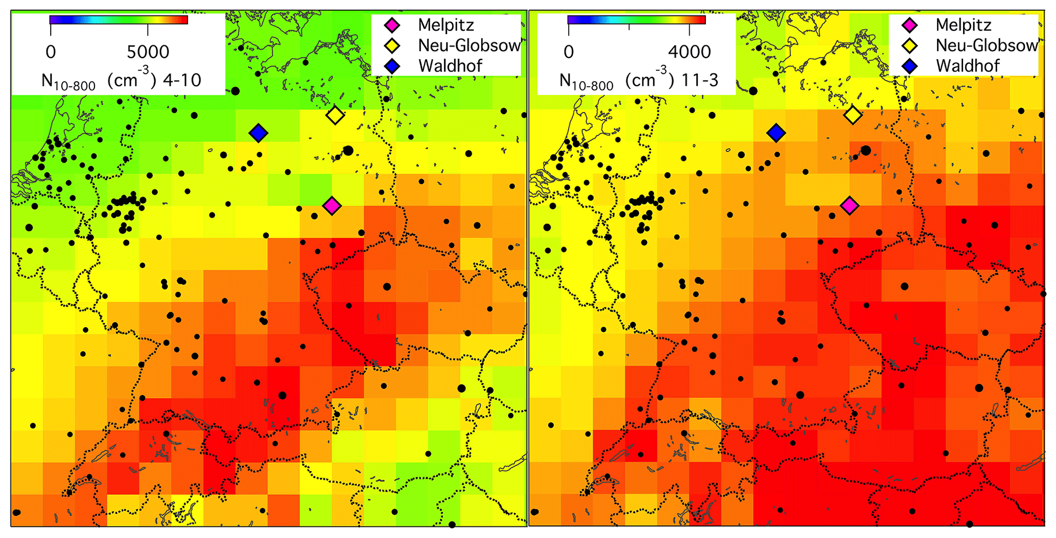
Figure 1 Maps of particle number concentration N₁₀₋₈₀₀ (cm⁻³) extrapolated under 1000 m of height along 5 d back trajectories from hourly data at the four stations from 2009 to 2018; left: months April through October; right: months November through March. The GUAN stations are marked with colored diamonds. The Collmberg station lies 30 km southeast of Melpitz station. Here and in the following maps the black dots represent cities larger than 100 000 inhabitants, with the size of the dots being proportional to the number of inhabitants.

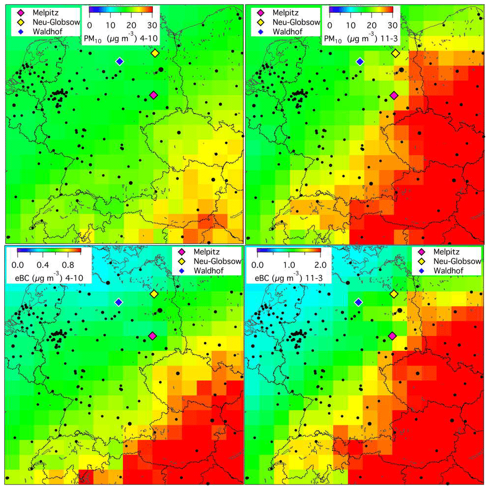
Figure 2 As Fig. 1 but for particle mass concentrations (top, PM₁₀; µg m⁻³) and black carbon concentrations (bottom, eBC; µg m⁻³).

The maps of N₁₀₋₈₀₀ in Fig. 1 show distributions of air masses over Germany and adjacent countries related to particle numbers instead of particulate mass. There are two arguments for showing maps of number-related results. First, particle number concentrations are connected with cloud processes, their formation (Pruppacher and Klett, 1978), radiative effects, e.g., albedo (Twomey, 1974), and precipitation (Li et al., 2011). Second, in the area of aerosol health issues, ultrafine particles (<100 nm diameter) have been gaining attention in recent years (Wichmann and Peters, 2000); i.e., an increasing number of health effects is attributed to particle number rather than to particle mass. The fact that NPF events occur concurrently in or near the top of the continental planetary boundary layer over wide geographical regions (e.g., Wehner et al., 2007) is partly due to concurrent advantageous photochemical conditions allowing for the formation of condensable vapors, in particular global radiation (Birmili et al., 2001). Two other factors constraining NPF are the availability of gaseous particle precursors and the concurrent preexisting aerosol.

The summer map (4-10) of N₁₀₋₈₀₀ exhibits high values in the southwest to northeast sector of the map. The highest values are concentrated in a belt reaching from Burgundy through Switzerland, southern Germany, and the Czech Republic to southwestern Poland. Interestingly, this belt of high N₁₀₋₈₀₀ is collocated to large extent with a belt of high summer ozone concentrations (see Fig. S1 in the Supplement). This photochemically controlled pollutant (Monks et al., 2015) exhibits the highest summer concentrations in air masses from southwestern Poland and the northern Czech Republic, a region from which high ozone values are reported (Struzewska and Jefimow, 2013; Hůnová, 2003; Hůnová and Bäumelt, 2018). However, the summer map of N₁₀₋₈₀₀ does not show the highest values in air masses from the region with the highest ozone pollution. High particle numbers in air masses coming over the Alps from northern Italy may be related to the high emissions of air pollutants in the Po Valley that are known to be reached frequently through so-called alpine pumping (Winkler et al., 2006; Lugauer and Winkler, 2005; Reitebuch et al., 2003) over the mountains. The high NO_x concentrations in air masses from northern Italy in both the summer and winter maps (see Fig. S2 in the Supplement) indicate that pollution from south of the Alps can even reach northeastern Germany. In the winter map of N₁₀₋₈₀₀ (11-3 in Fig. 1) the belt of highest summer values is apparently complemented by more transalpine pollution transport and by transport from the southeast. The lower photochemical activity in winter is reflected in the lower winter ozone concentrations in Fig. S1 in the Supplement, although transalpine pollution transport is still visible in the winter map of NO_x in Fig. S2 in the Supplement. Northwestern Italy also shows up as an emission hot spot in the maps of trajectory-summed emissions in Fig. S4 in the Supplement.

In both summer and winter the maps of PM₁₀ and eBC in Fig. 2 exhibit a clear northwest-to-southeast structure with the cleanest sector being in the northwest, covering the coastal area of the North Sea and the BENELUX countries Belgium, the Netherlands, Luxembourg, and northwestern Germany. The strongest contrast between the cleanest northwesterly and the most polluted southeasterly map sectors is seen in the winter map of eBC. The highest average concentrations are measured in air masses from the southeastern half of the map, most strongly expressed in PM₁₀ and eBC with maxima in a region leading from southwest Poland through the Czech Republic, Slovakia, Austria, and former Yugoslavia to northeastern Italy. The back trajectories in the southeastern sector of the maps for PM₁₀ and eBC point towards countries in which emissions of air pollution in the past 20 years developed very differently compared to those in western Europe. According to the European Environment Agency (https://www.eea.europa.eu/data-and-maps/dashboards/air-pollutant-emissions-data-viewer-2, last access: 18 September 2020) parts of western Europe experienced a strong and nearly monotonous decrease in emissions of PM₁₀, whereas the emissions in Poland, the Czech Republic, Slovakia, Austria, former Yugoslavia, and Italy stayed nearly constant or even increased in recent years after dramatic decreases in the course of political developments of the 1990s. The seasonal maps of combustion-derived SO₂ in Fig. S3 in the Supplement look very similar to the those of the particle-mass-related maps of PM₁₀ and eBC, again with the strongest NW–SE contrast visible in winter.

5.2 Pollutant emissions and atmospheric processes

In Fig. 3 annual average emissions of PM₁₀, BC, SO₂, and NO_x are mapped for 2009 according to EDGAR. Except for the absolute numbers, the maps for SO₂ and NO_x look rather similar to those for particulate emissions. They all emphasize highly populated and industrialized emission centers. Beyond that, the SO₂ map accentuates individual large combustion sources such as conventional power plants. Whereas the strong emissions in northern Italy are seen in the maps of PM₁₀, BC, and NO_x, emissions in the countries in the southeastern sector of the maps by no means reflect the high concentrations of particulate components seen in the pollution maps in Figs. 1 and 2.

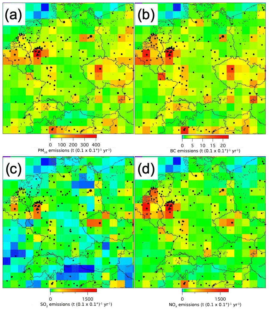
Figure 3 As Fig. 1 but (a) for PM₁₀ emissions ($\mathrm{t}(\mathrm{0.1}\times \mathrm{0.1}{}^{\circ }{)}^{-\mathrm{1}}{\mathrm{yr}}^{-\mathrm{1}}$), (b) BC emissions, (c) SO₂ emissions, and (d) NO_x emissions ($\mathrm{t}(\mathrm{0.1}\times \mathrm{0.1}{}^{\circ }{)}^{-\mathrm{1}}{\mathrm{yr}}^{-\mathrm{1}}$) according to EDGAR (https://doi.org/10.2904/JRC_DATASET_EDGAR) for 2009 averaged over the geogrid of the present study.

The seeming discrepancy between the pollution maps in Figs. 1 and 2 and the emission maps in Fig. 3 can be resolved. For that purpose, the EDGAR emissions of PM₁₀, BC, SO₂, and NO_x along all 350 593 hourly back trajectories to the four stations during the 10 studied years were summed up. Then the sums were extrapolated back along each trajectory. In Fig. S4 in the Supplement 10-year average maps of these extrapolated emission sums are displayed. As in Fig. 3, except for the absolute numbers, there is a strong similarity between the four mapped component sums. Because of the integral nature of the mapped results one cannot expect the maps in Fig. S4 to correctly locate specific emission centers. However, they certainly indicate the map sectors from which the most substantial emissions could have reached the stations. As in Figs. 1 and 2 the southeastern sectors of the maps of integrated emissions most prominently show up. Interestingly, the maps in Fig. S4 in the Supplement also indicate the highly polluted region of northwestern Italy (Diémoz et al., 2019a, b). Emissions from the emission centers in northwestern Europe are hardly discernible in Fig. S4 in the Supplement. They do show up (most strongly in Fig. S4c in the Supplement for SO₂ emission sums) as apparent emissions over the adjacent North Sea. We interpret the “misplaced” emissions over the North Sea as air mass transport from the North Sea via the emission region in the BENELUX countries to the receptor sites that was not compensated for by other low-pollution air transport from the North Sea to the stations that had not passed over the northwestern European emission centers.

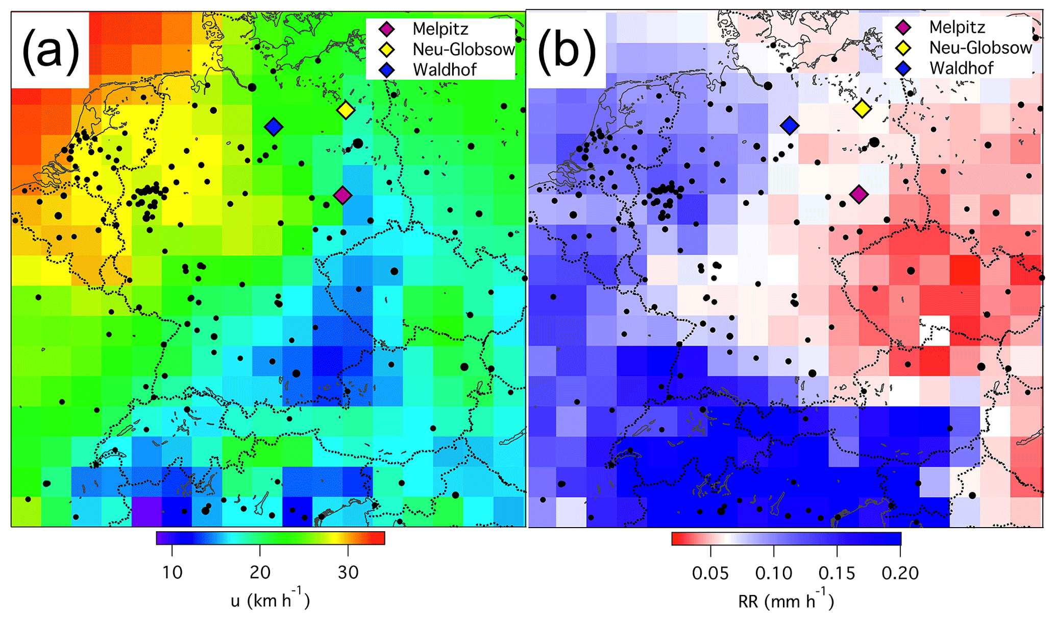
Figure 4 (a) Map of horizontal wind speed (u, km h⁻¹) as reported by HYSPLIT along hourly 5 d back trajectories to the four stations marked in the graph averaged over the time period 2009 to 2018; (b) as (a) but for precipitation (RR, mm h⁻¹).

Two major atmospheric processes will reduce the concentrations of emitted or in situ formed aerosol particles: dilution through mixing with cleaner air masses and wet scavenging through in-cloud and sub-cloud processes. As a tracer of the first of these two processes, Fig. 4a gives the long-term average geographical distribution of trajectory-derived wind speed over the study area. The highest average wind speeds and ensuing atmospheric mixing are seen over the major emission centers of northwestern Germany, the BENELUX countries, and adjacent seas, whereas the lowest wind speeds are seen over northern Germany and the southeastern neighboring countries. The long-term average geographical distribution of precipitation as taken by HYSPLIT from the GDAS meteorological fields in Fig. 4b corroborates the results for atmospheric cleaning processes indicated in Fig. 4a. The small absolute numbers in Fig. 4b are due to the episodic nature of precipitation: most of the time it does not rain or snow. The blue crescent reaching from the North Sea through the BENELUX countries, eastern France, Switzerland, and the alpine region exhibits maximum precipitation values, while southern and eastern Germany with the adjoining countries to the east and southeast show minimum precipitation values. Thus, in the long term we expect much of the high western European emissions to be substantially scavenged by wet processes. In addition, air masses arriving from western and northwestern directions at the stations usually cross the western European emission centers with much lower pollution burdens than air masses coming from the polluted countries of southeastern Europe arriving at the corresponding map borders (see the figure labeled PM₁₀ – 36th maximum daily average value (µg m⁻³) for 2005; EEA, 2009).

5.3 Pollution trends for air from specific source regions

As mentioned in the Introduction, the pollutant emissions reported by European and national environment agencies represent a synthesis of known pollutant sources combined with assumed emission factors. These emissions are typically used as input for air quality modeling and subsequent assessment, as well as for trend analyses. However, it remains unclear to what extent these reported emissions are realistic and whether their trends represent the trend in true emissions. Here, we attempt to assess spatially resolved trends in real particulate emissions by an analysis of measured concentrations (pollution) in air masses traveling over source-specific regions.

To test our method, we selected two pronounced source regions in Europe located within 1000 km of distance from our observation sites. These regions were defined by emission hot-spot regions that can be seen in the EDGAR emission maps in Fig. 3a and b: region A (Be-NL-NRW; comprising most of Belgium, southern parts of the Netherlands, and much of the German state North Rhine-Westphalia) and region B (CZ-PL-SK; comprising the central parts of the Czech Republic, southern parts of Poland, and adjacent areas of Slovakia). According to the European Environment Agency (EEA) these are regions where reported particulate emissions have developed differently during the past 10 years. Our goal is to verify this through an analysis of real atmospheric observations over this period.

Temporal trends were computed using the customized Sen–Theil trend estimator (Sen, 1968; Theil, 1992). The Sen–Theil estimator is the median of many slopes calculated in a continuous or noncontinuous time series, with its robustness against outliers being one of its main assets. For a detailed description of this trend estimator we refer to Sun et al. (2020, Sect. 2.3.1). Here we computed the Sen–Theil estimator for hourly observation data at stations ME, NG, and WA. Subsets of back trajectories were selected that spent at least 1, 3, 6, or 12 h over source regions A and B. Depending on that criterion, different subsets were analyzed. The difference in median eBC mass concentration between air masses arriving from source region A and B is obvious, as could already be determined in the corresponding pollution maps (Fig. 2c and d). As we learned from Sect. 5.2 these pollution maps are strongly influenced by the different meteorological conditions governing atmospheric dispersion in different wind directions, so these values allow no direct conclusion on the strength of emission sources located upwind.

Table 2 Median concentrations of eBC (µg m⁻³) and temporal trends (2009–2018) of eBC in terms of Sen–Theil slope (% yr⁻¹) as determined for air masses passing over regions A and B as analyzed at the stations Melpitz (ME), Neuglobsow (NG), and Waldhof (WA). For comparison the national annual decreases in BC emissions for 2009–2017 in percent according to the European Environmental Agency are added.

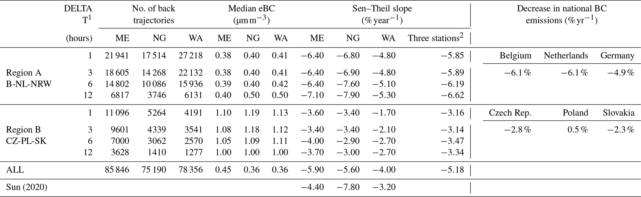
¹ Minimum time spent over the specified source region. ² Weighted mean according to the available number of back trajectories.

We analyzed the temporal trends in eBC over the period 2009–2018 for the subsets belonging to regions A and B – assuming that these systematic differences in meteorological conditions should even out over such long observation periods. Table 2 shows that the Sen–Theil slope estimator for region A is between −7.6 % and −5.1 % for the three observation sites and the requirement of a back trajectory to have spent at least 6 h over region A. For region B, the corresponding Sen–Theil slope estimators are between −4.0 % and −2.7 % for the observation sites. As we can read from these results, the annual decrease in eBC is more pronounced for air masses that have traveled over region A.

Table 3 Percental decreases in anthropogenic emissions of PM₁₀, BC, SO₂, and NO_x relative to 2009 as reported by the European Environment Agency (EEA, https://www.eea.europa.eu/data-and-maps/dashboards/air-pollutant-emissions-data-viewer-2), the German Environment Agency (GEA), and calculated in the present study. The EEA and GEA only report data until 2017.

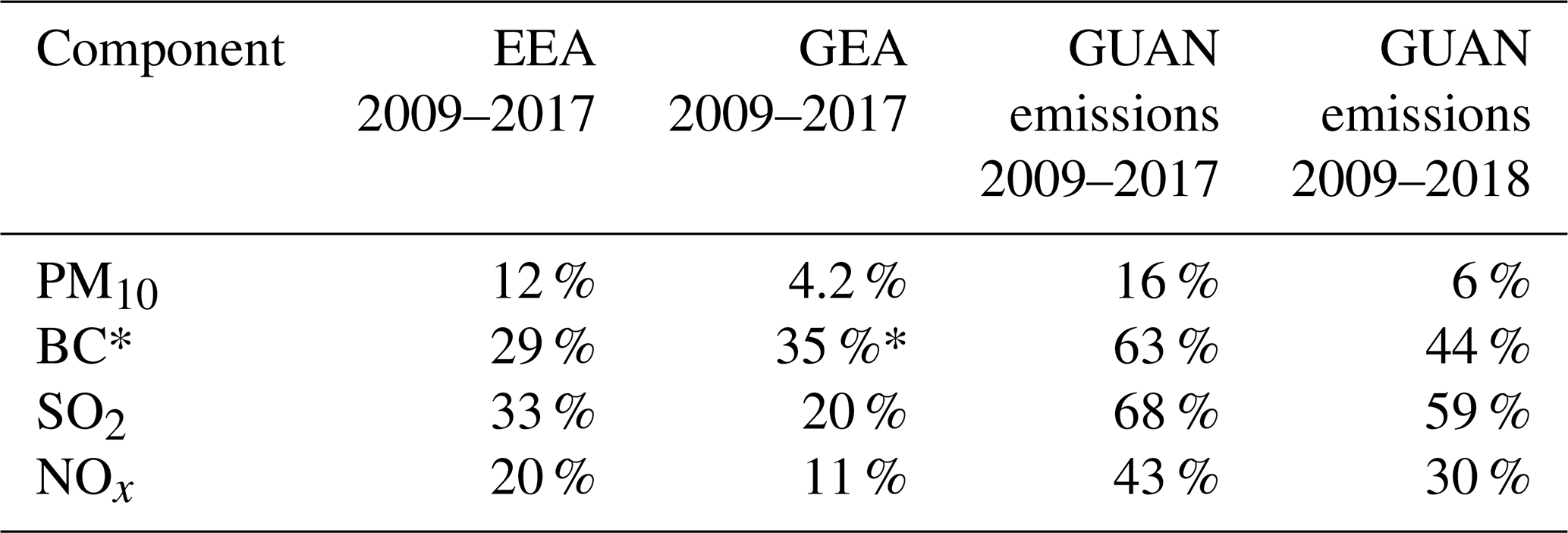
* BC until 2016.

Between 2009 and 2017 for the EU member states of Belgium, the Netherlands, Germany, the Czech Republic, Poland, and Slovakia the annual rates of decrease in reported emissions were between −4.9 % and −6.1 % for the first three countries and between +0.5 % and −2.8 % for the latter three (https://www.eea.europa.eu/data-and-maps/dashboards/air-pollutant-emissions-data-viewer-2). As compiled in Table 3 these reported trends are largely consistent with the rates of change derived from our eBC pollution trends. Although we need to keep in mind that the six nations only partially contribute to our regions A and B, it seems valid to conclude that BC emissions in region A indeed decreased more rapidly in the past decade compared to region B. Our approach seems able to differentiate between concentration trends in air masses that have passed over rather different source regions. This might represent a step towards the assessment of changes in real-world emissions allocated in specific source regions over multi-annual periods.

5.4 Comparison of pollution and emission trends

Besides the map comparison a second approach was used to connect emission data with the measured aerosol time series. Along each of the hourly back trajectories the emissions according to EDGAR were summed up. Then monthly medians of the emission sums and the measured parameters were formed. EDGAR reports annual average emissions. PM₁₀, black carbon, and other combustion-related air pollutants show substantial annual variations, with high winter and low summer values at nonurban sites (e.g., Heintzenberg and Bussemer, 2000). In emission modeling the temporal variation of annually reported emissions is considered by disaggregating the annual values with monthly, weekly, and daily factors (Matthias et al., 2018). For the time-resolved comparison of PM₁₀ and BC emissions with PM₁₀ and eBC concentrations at the GUAN sites, monthly medians of PM₁₀ and eBC values at the stations were formed and plotted in Fig. 5. We expected both seasonal variations and a long-term trend in the emissions. For M hours per month of measured components at the four stations the annual average EDGAR emissions $E_{\text{PM10}},E_{\text{BC}},E_{\text{SO2}}$, and E_NOx were summed up along the 121 trajectory steps leading to the stations. Then monthly medians ${\stackrel{\mathrm{̃}}{E}}_{i=\mathrm{1},\mathrm{4}}$ were formed according to Eq. (1) (exemplified for BC). Medians were chosen to reduce the effect of outliers due to local emission and scavenging events.

$$\begin{array}{}\text{(1)}& {\displaystyle }{\stackrel{\mathrm{̃}}{E}}_{\text{BC}}=\text{Median}{\left(\sum _{n=\mathrm{1}}^{\mathrm{121}}{E}_{\text{BC}}\right)}_{m=\mathrm{1},M}\end{array}$$

The monthly median emission sums ${\stackrel{\mathrm{̃}}{E}}_{i=\mathrm{1},\mathrm{4}}$ were modified with a monthly (f_m) and an annual factor (g_y) in order to simulate respective median monthly measured concentrations taken over all stations. Thus, for each component 12 monthly and 10 annual trend factors determined the agreement of modified summed emissions and measured concentrations. As an objective or utility function, χ², the sum of squared deviations between annually and monthly modified emission sums and monthly median measured concentrations, was formed taken over the 120 months of the present study (exemplified for BC in Eq. 2).

$$\begin{array}{}\text{(2)}& {\displaystyle }{\mathit{\chi }}_{\text{BC}}^{\mathrm{2}}=\sum _{j=\mathrm{1}}^{\mathrm{120}}{\left(f_{m=\mathrm{1},\mathrm{12}}\times g_{y=\mathrm{1},\mathrm{10}}\times {\stackrel{\mathrm{̃}}{E}}_{\text{BC}}-\mathrm{eBC}\right)}^{\mathrm{2}}\end{array}$$

χ² was minimized with a generalized reduced gradient (GRG) solver (Lasdon et al., 1978) that optimized the 12 monthly and 10 annual factors for each of the four measured components. We used Excel's^® implementation of the GRG solver procedure for the optimization. After optimizing month and trend factors the average relative deviation between emission-simulated and measured monthly median curves is 14 %, 21 %, 25 %, and 18 % for PM₁₀, eBC, SO₂, and NO_x, respectively. The optimized monthly median emission sums for all four parameters are displayed in Fig. 5 together with the measured monthly median concentrations.

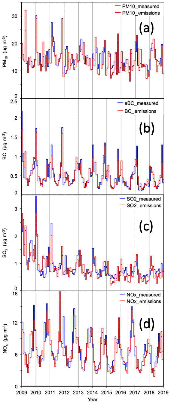
Figure 5 (a) Monthly medians of PM₁₀ concentrations at the four stations in the present study (blue) and monthly medians of optimized sums of PM₁₀ emissions along back trajectories leading to the stations (red). Panel (b) is as (a) but for measured eBC concentrations and BC emissions along back trajectories. Panel (c) is as (a) but for measured SO₂ concentrations and SO₂ emissions along back trajectories. Panel (d) is as (a) but for measured NO_x concentrations and NO_x emissions along back trajectories.

A 10-year trend in emissions of PM₁₀, BC, SO₂, and NO_x, as well as average monthly factors for the respective parameters are the two essential results derived from the optimization approach. The 10-year trends relative to 2009 are collected in Fig. 6. Annual averages of the relative differences between the monthly median measured parameters and the corresponding emission-derived parameters were formed and applied to the GUAN trend values displayed in Fig. 6. The resulting error bars on the trends serve as estimates of the uncertainties of the optimization approach. The general trend in Fig. 6 is downward to minima between 30 % and 70 % of the 2009 values in 2016–2017 after which all parameters exhibit increases, most strongly PM₁₀. SO₂ shows the strongest decrease, whereas PM₁₀ and NO_x emissions diminished the least. In 2010–2011 the trend curves of PM₁₀ and NO_x in Fig. 6 show a slight increase that can be linked to a recovery of economic activity after the worldwide financial and economic crisis during the period 2007-2009. The increase in PM₁₀ is also visible in the trend curves relative to 2005 published by the German Environment Agency (https://www.umweltbundesamt.de/daten/luft/luftschadstoff-emissionen-in-deutschland/emissionen-prioritaerer-luftschadstoffe, last access: 18 September 2020).

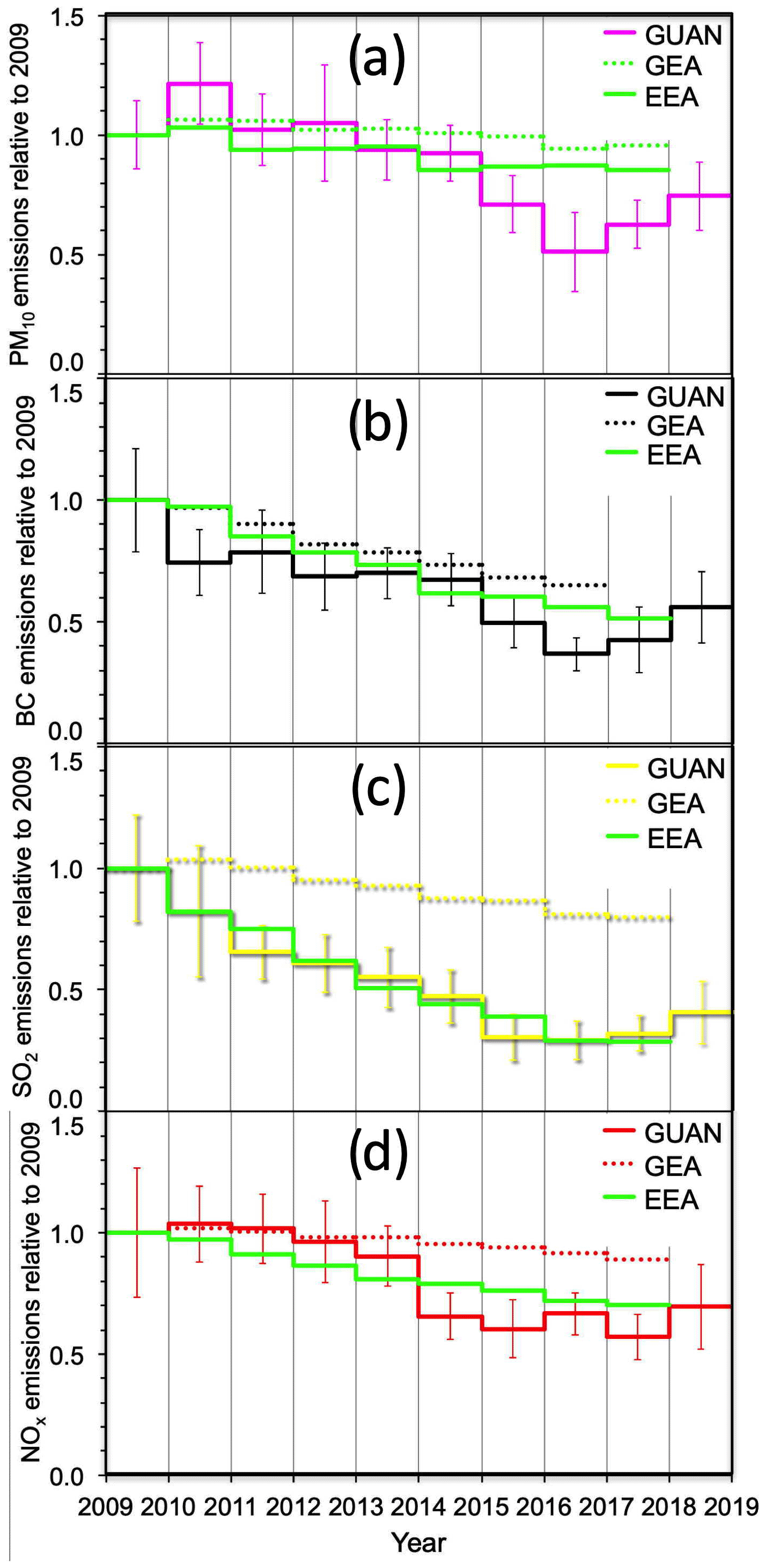
Figure 6 GUAN: trends in the emissions of (a) PM₁₀, (b) BC, (c) SO₂, and (d) NO_x relative to 2009 as calculated by optimizing the agreement between 2009 EDGAR emissions and concentrations measured at the four stations in the present study. The error bars represent annual average relative deviations between measured and simulated data. GEA: trends as reported for Germany by the German Environment Agency. EEA: trends as optimized from combinations of trends over Germany and neighboring countries (see the text for details).

The results of two comparisons of our trends with data reported by the German and European environment agencies are added to Fig. 6. In general, the trends reported by the German Environment Agency for all German emissions exhibit weaker reductions than the results of the present study. Only for PM₁₀ in 2011 and 2013 does the present study yield higher values than GEA. We note that primary PM₁₀ emissions may have substantial contributions from wind erosion of agricultural soils (Panagos et al., 2015) that are not incorporated in present anthropogenic inventories. SO₂ exhibits the strongest trend discrepancies, with much stronger reductions of the trend in the present study compared to GEA results. As Germany has been reducing SO₂ emissions systematically since the 1980s one would not expect any further strong trends during the time period of the present study. As other studies have demonstrated before (e.g., van Pinxteren et al., 2019), the maps in Fig. 1 indicate the possibility of imported pollution, in particular from the southeast. Consequently, we searched for similar trends in emission data reported by the EEA for neighboring countries until 2017 directly west, south, and east of Germany, going east all the way to Romania. Excel's solver optimized combinations of the EEA trends for Germany and neighboring countries in order to fit the trends derived in the present study. The solver did not choose German trends for any of the four parameters PM₁₀, BC, SO₂, and NO_x. For PM₁₀ a combination of emission trends for the BENELUX countries and France was optimum, albeit without being able to simulate the relative maxima in 2011 and 2013 and the minimum around 2016. For BC the emission trend for the BENELUX countries came closest to the trend of the present study. For SO₂, emissions in Romania, with minor contributions from French and BENELUX trends, simulated the trends observed over Germany best. NO_x trends were best simulated by emissions over the Czech Republic and Slovakia. Emissions trends over Switzerland, Austria, Hungary, and Poland were not utilized by the solver. All simulated trends are displayed as curves in Fig. 6. We do not claim that these simulated trends numerically correspond to imported pollution over Germany. However, the good fit of the SO₂ trend to emissions over Romania corroborates our finding of pollution import from southeastern Europe to northeastern Germany, while the development of BC appears to better follow emission trends over western neighboring countries than over Germany.

Sun et al. (2020) investigated trends of size-resolved number and eBC mass concentrations at 16 observational sites in Germany from 2009 to 2018, including the three GUAN sites in the present study. Based on monthly median time series they report average decreases for ME, NG, and WA of −5.5 %, −6.1 %, and −3.9 %, respectively. The corresponding result for eBC in the present study is −4.6 %, albeit with a high variability (see Fig. 6) of 20 % units expressed in terms of an SD.

Over the polluted continent the particle-number-based parameter N₁₀₋₈₀₀ is largely secondary in nature; i.e., its concentrations are controlled by atmospheric constituents and processes. Thus, there is no primary emission database with which a similar trend analysis as with PM₁₀, BC, SO₂, and NO_x could be attempted. Instead we chose the 10-year grand averages (GAs) taken over the whole time period of the present study as references from the deviations of annual averages are discussed. Sun et al. (2020) report very minor trends (between −3.5 % and 0.1 %) for N₂₀₋₈₀₀ at the three GUAN stations used in the present study. The 10-year interannual variation of our N₁₀₋₈₀₀ in Fig. 7a bears out why only a minor trend if any can be expected. For the first 4 years the annual averages are substantially higher than average. Then annual values decrease down to a minimum in the years 2016–2017 before they increase again to a level slightly above the 10-year average.

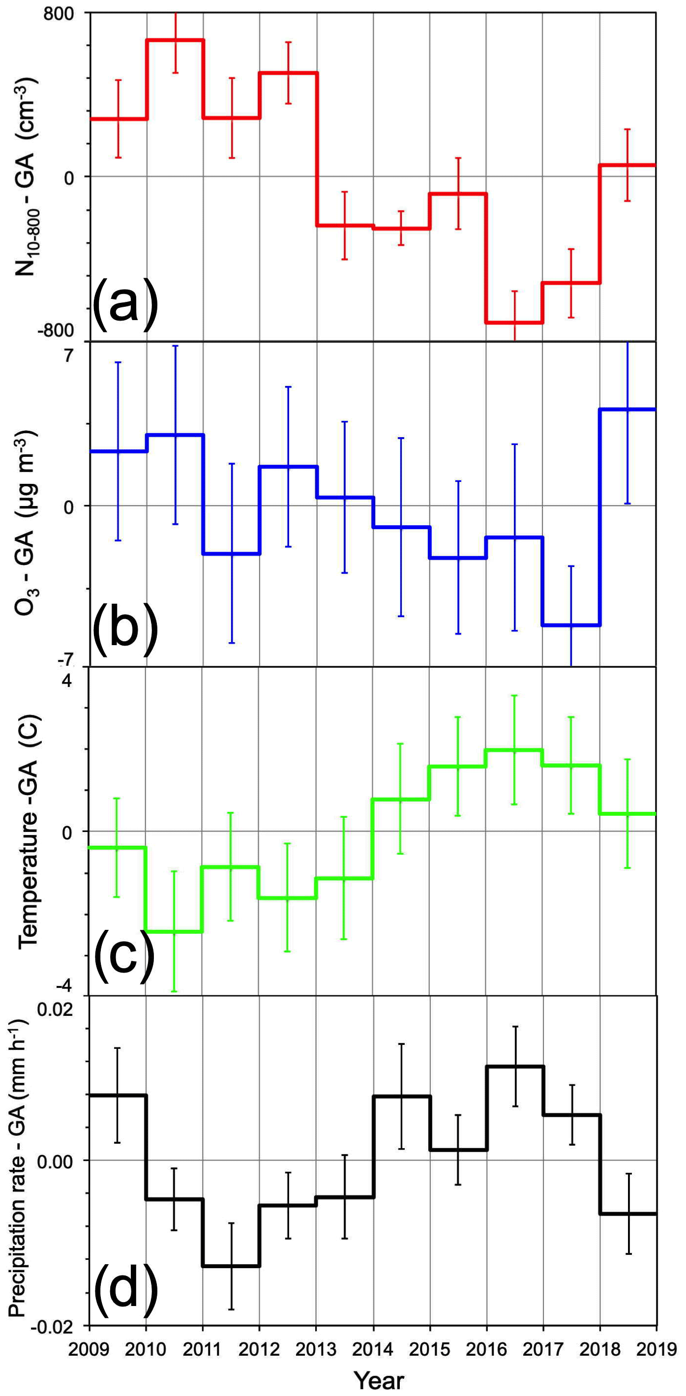
Figure 7 Trends in annual average deviations of (a) ΔN₁₀₋₈₀₀, (b) ΔO₃, and (c) temperature ΔT along the trajectories 5 d back in time, as well as (d) precipitation rate ΔRR along the trajectories 3 d back in time. The deviations are taken relative to the respective 10-year grand average (GA). The error bars represent the SDs of the annual averages.

In Fig. 7b–d annual deviations from the respective GAs are displayed that can be connected to the 10-year course of N₁₀₋₈₀₀. Ozone concentrations averaged over the data from the three GUAN stations can be interpreted as an indicator for photochemical activity that also controls NPF. The annual deviations of O₃ in Fig. 7b rather closely follow those of N₁₀₋₈₀₀. In Fig. 7c and d annual deviations of ambient temperature and precipitation rates are displayed that have been averaged over the meteorological data along the back trajectories leading to the four stations. For the temperature an averaging period of 120 trajectory hours yielded the highest (negative) correlation with N₁₀₋₈₀₀ of $r=-\mathrm{0.8}$. After a dip in 2009 annual average trajectory temperatures reached a maximum in 2016 before returning to near average in 2018. For the precipitation rates along the trajectories the highest (negative) correlation with N₁₀₋₈₀₀ was found with an averaging period of 3 d ($r=-\mathrm{0.6}$) before arrival at the stations. The results displayed in Fig. 7c and d illustrate the complexity of the processes and conditions controlling atmospheric particle number concentrations. On one hand, a scavenging effect of precipitation can be used as an argument for the high values of N₁₀₋₈₀₀ in the years 2010–2013 and the low values in the years 2014 through 2018. On the other hand, lower annual temperatures during years of relatively high N₁₀₋₈₀₀ and higher-than-GA temperatures during years of relatively high N₁₀₋₈₀₀ are harder to interpret. Possibly, the nucleation of condensable vapors is furthered by lower air temperatures upwind of the stations.

An important result of trend analysis is the average monthly factors disaggregating the annual emissions. In general the summer minima of the month factors determined in the present study are broader than the curve given by Matthias et al. (2018) for combustion emissions. The decrease in the month factor of PM₁₀, BC, and NO_x in December and the late winter maxima of PM₁₀ and SO₂ are not reflected in the Matthias et al. (2018) results. Interestingly, both PM₁₀ and SO₂ show a minor secondary peak in June. As an example of the seasonal variability of eBC within an urban source region we averaged the relative annual variation of eBC concentrations at the station Leipzig Eisenbahnstraße (plotted as curve L-EBS in Fig. 8), exhibiting a smaller seasonal swing than all other curves. The curve for PM₁₀ comes closest to that for L-EBS, probably because of agricultural noncombustion emissions in summer.

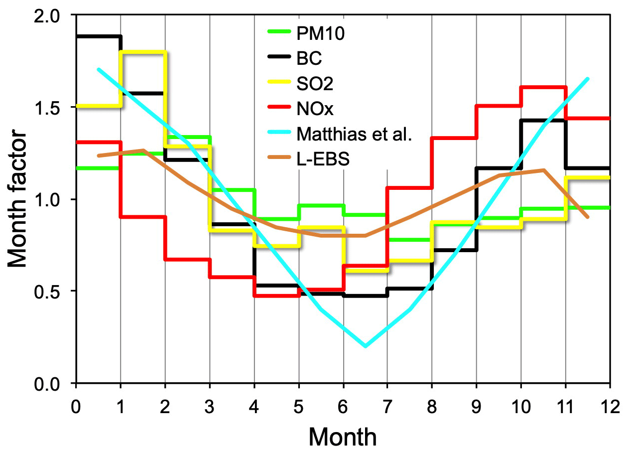
Figure 8 Month factors for emissions of PM₁₀, BC, SO₂, and NO_x as determined by optimizing the agreement between EDGAR emissions and concentrations measured at the four stations in the present study. For comparison the month factors of Matthias et al. (2018) for combustion emissions are plotted, and the relative annual variation of eBC concentrations measured at the station Leipzig Eisenbahnstraße (L-EBS) are averaged over the time period of the present study.

In general the downward trends in particulate parameters determined in the present study are similar to temporal trends of particle number and black carbon mass concentrations at 16 observational sites in Germany from 2009 to 2018 (Sun et al., 2020). The long-term emission decrease in PM₁₀ as determined in the present study from 2009 to 2018 is smaller than the corresponding number published by the EEA as an average over all 28 EU member states but similar to the figures published by the GEA through 2017 (see Table 3). For BC, SO₂, and NO_x the present study yields substantially stronger emission reductions than both the GEA and EEA. These findings are emphasized when considering 2017 to be the end point of the trend calculation (see Table 3) at and after which our study shows consistent emission increases of all studied parameters. Comparing the calculated trends with emission trends in neighboring countries as published by the European Environment Agency supports the explanation that the observed trends are to some extent due to changes in imported air masses. This holds most strongly for SO₂, the trend of which follows that of Romanian emissions rather well.

The last issue we take up in this discussion concerns the frequent residual difference between measured and emission-simulated time series. In Fig. 5, e.g., in most winters, there are months when optimized BC emissions remain substantially lower than the measured monthly medians of eBC. Some information can be gleaned from the “Großwetterlagen” (GWL), representing 29 classifications of large-scale weather types after Hess and Brezowsky for central Europe (Gerstengarbe and Werner, 1993), provided by the German Weather service for each day (http://www.dwd.de/DE/leistungen/grosswetterlage/grosswetterlage.html, last access: 18 September 2020). During the winter months with the strongest difference between measured and simulated time series the probabilities of high-pressure systems over Fennoscandia with south-to-southeasterly flow to the four stations are substantially higher than the respective probabilities averaged over the whole 10-year period of the study. This GWL information is consistent with the back trajectories during the high-pollution winter months coming predominantly from the southeasterly sector of the map. While the classified large-scale weather situation with weak dilution of pollution during the winter months is conducive to high particulate concentrations at the receptor sites, it does not explain the discrepancy. In principle our simplistic approach of accumulating emissions along back trajectories may be flawed during certain weather situations. However, an alternative explanation could be that the emissions inventories over eastern and southeastern Europe in EDGAR are somewhat lower than the real emissions.

6 Summary and conclusions

A total of 10 years of hourly aerosol and gas data at three stations of the German Ultrafine Aerosol Network (GUAN) and one station of the Saxonian Environment Agency have been combined with hourly back trajectories to the stations and emission inventories. Measured PM₁₀, particle number concentrations between 10 and 800 nm, and equivalent black carbon were extrapolated along the trajectories. This process yielded what we termed pollution maps of these aerosol parameters over Germany. They reflect aerosol emissions modified with atmospheric processes along the air mass transport between sources and the four receptor sites at which the potential effects of particulate air pollution would be realized.

The 10-year average pollution maps do not simply show the distribution of pollution sources upwind of the receptor sites. The comparison with emission data based on the European EDGAR shows that strong western European emission centers do not dominate the downwind concentrations because their emissions often are reduced by wet scavenging and dilution processes on the way to the receptor area. Maps of average precipitation and wind as they occurred along the trajectories illustrate these processes. In the receptor region mass-related aerosol parameters, such as PM₁₀, equivalent black carbon, and to some extent also the particle number concentration, are instead rather controlled by emissions from eastern and southeastern Europe from which pollution transport often occurs under drier meteorological conditions in continental high-pressure air masses. This finding corresponds to the air mass results derived for the submicrometer particle number size distribution by Birmili et al. (2001), by Engler et al. (2007) for the size distribution of non-volatile particles, by Ma et al. (2014) for optical particle properties all evaluated at the Melpitz station, and by van Pinxteren et al. (2019) for the transboundary transport of PM₁₀ to 10 stations in eastern Germany from neighboring countries. Newly formed particles, on the other hand, are found in air masses from a broad belt reaching from Burgundy to the western Czech Republic and southern Poland, a region with high photochemical activity in summer that is affected by emissions in northern Italy.

Annual EDGAR emissions for 2009 of PM₁₀, BC, SO₂, and NO_x were accumulated along each trajectory and compared to the calculated emission sums with the corresponding measured time series on a monthly basis. With a generalized reduced gradient solver the agreement of each pair of monthly time series, e.g., measured eBC and BC emissions, was optimized by letting the solver determine both monthly emission factors disaggregating the annual EDGAR emission fields and adjusting the emissions with annual factors modifying the 2009 fields. Relative to 2009 the annual averages of the analyzed air pollutants were lower in 2018 by values between 6 % for PM₁₀ and 60 % for SO₂. In general, the 10-year reductions determined in the present study were stronger than those reported by the German and the European environmental agencies. N₁₀₋₈₀₀ exhibited substantial interannual variability but no net decrease over the 10 studied years.

The validity of the present approach of connecting the ambient concentration and emission of particulate pollution was tested by calculating temporal changes in eBC for subsets of back trajectories passing over two separate prominent emission regions, region A to the northwest and B to the southeast of the measuring stations. Consistent with reported emission data the calculated pollution decreases over region A are significantly stronger than over region B.

Compared to published emission monthly factors by Matthias et al. (2018) the present approach yielded broader summer minima that were partly displaced from the midsummer positions given by Matthias et al. (2018). As an aside we note that during the winter months with extremely high particulate pollution the emissions accumulated along back trajectories are often substantially lower than the measured concentrations, which raises the question of the validity of the emission figures in eastern and southeastern European source regions.

There are clear limits to the methodology in the present study. Air mass trajectories have inherent uncertainties that increase with their distance traveled (Stohl, 1998). Meteorological processes affecting aerosol during air mass transport are only considered rather coarsely, whereas aerosol dynamics are not considered at all. Possible future improvements concern ensemble trajectories with higher resolution, better meteorological information along the trajectories, e.g., radar-derived precipitation as used in Heintzenberg et al. (2018), more comprehensive emission inventories with higher spatiotemporal resolution, and higher numbers of analyzed stations.