Small-scale variability of stratospheric ozone during the sudden stratospheric warming 2018/2019 observed at Ny-Ålesund, Svalbard

Middle atmospheric ozone, water vapour and zonal and meridional wind profiles have been measured with the two ground-based microwave radiometers GROMOS-C and MIAWARA-C. The instruments have been located at the Arctic research base AWIPEV at Ny-Ålesund, Svalbard (79^∘ N, 12^∘ E), since September 2015. GROMOS-C measures ozone spectra in the four cardinal directions with an elevation angle of 22^∘. This means that the probed air masses at an altitude of 3 hPa (37 km) have a horizontal distance of 92 km to Ny-Ålesund. We retrieve four separate ozone profiles along the lines of sight and calculate daily mean horizontal ozone gradients which allow us to investigate the small-scale spatial variability of ozone above Ny-Ålesund. We present the evolution of the ozone gradients at Ny-Ålesund during winter 2018/2019, when a major sudden stratospheric warming (SSW) took place with the central date at 2 January, and link it to the planetary wave activity. We further analyse the SSW and discuss our ozone and water vapour measurements in a global context. At 3 hPa we find a distinct seasonal variation of the ozone gradients. The strong polar vortex during October and March results in a decreasing ozone volume mixing ratio towards the pole. In November the amplitudes of the planetary waves grow until they break in the end of December and an SSW takes place. From November until February ozone increases towards higher latitudes and the magnitude of the ozone gradients is smaller than in October and March. We attribute this to the planetary wave activity of wave numbers 1 and 2 which enabled meridional transport. The MERRA-2 reanalysis and the SD-WACCM model are able to capture the small-scale ozone variability and its seasonal changes.

1 Introduction

In the Arctic, the polar vortex dominates the dynamics of the wintertime middle atmosphere. The polar vortex is a cyclonic wind system which forms in autumn from the balance between the Coriolis force and the pressure gradient force between the pole and the midlatitudes, which results from the radiative cooling of the polar middle atmosphere in the absence of solar heating. The polar vortex maintains a transport barrier between polar and midlatitude air which leads to gradients in trace gas concentrations across the polar vortex edge. Interactions of enhanced planetary waves with the mean flow can disturb this stable wind system (Matsuno, 1971) and cause a sudden stratospheric warming (SSW, Scherhag, 1952), which is one of the most dramatic meteorological phenomena in the middle atmosphere. Thereby the polar vortex can shift off the pole or even split into two or more sub-vortices (Charlton and Polvani, 2007). The zonal mean wind reverses and in the stratosphere adiabatic descent leads to temperature increases up to 60 K or more within a few days, whereas in the mesosphere adiabatic ascent leads to temperature decreases (e.g. Hocke et al., 2015; Manney et al., 2009). Meridional transport and irreversible mixing across the polar vortex edge are enhanced during an SSW (Calisesi et al., 2001; Manney et al., 2009; Tao et al., 2015; de la Cámara et al., 2018).

Changes in dynamics and temperature during an SSW lead to drastic changes in the distribution of trace gases like ozone and water vapour. Ground-based microwave radiometry provides continuous profile measurements of these trace species and horizontal winds in the middle atmosphere with a high time resolution of the order of hours for the trace species and 1 d for wind. It is therefore a valuable technique for the investigation of the temporal changes in trace gas concentrations and dynamics on small timescales.

During an SSW the polar vortex often moves away from the pole to the midlatitudes. In the Arctic, this leads to the advection of midlatitude air to the pole and sudden changes in the trace gas concentration. With ground-based microwave radiometry increases in stratospheric ozone of up to 100 % and increases in mesospheric water vapour of the order of 50 % were observed (Scheiben et al., 2012; Tschanz and Kämpfer, 2015; Ryan et al., 2016; Schranz et al., 2019). Traces of SSWs were also observed at the midlatitudes. At Bern, Switzerland, stratospheric ozone decreased by 30 % during the major SSW in 2008. In the lower stratosphere the polar vortex passed at Bern and the decrease is explained by the advection of ozone-poor polar vortex air. In the upper stratosphere the polar vortex did not reach Bern and the ozone decreased, mainly because increasing temperatures led to faster ozone destruction via the NO_x cycle (Flury et al., 2009). During the 2008 SSW an altered transport pattern led to an anticorrelation of mesospheric water vapour between Seoul, South Korea, and Bern, Switzerland (De Wachter et al., 2011). In Bern water vapour increased by 15 % (Flury et al., 2009), whereas at Seoul a water vapour decrease of 40 % was observed (De Wachter et al., 2011). The zonal wind reversals could be observed during several SSWs at midlatitudes and in the Arctic (Wang et al., 2019; Rüfenacht et al., 2014; Schranz et al., 2019).

The aforementioned studies observed a single profile per location and investigated the variability of trace species on small temporal scales. With the measurements from the GROMOS-C ground-based microwave radiometer we are for the first time able to investigate the variability of ozone on small spatial scales. GROMOS-C measures ozone spectra in the four cardinal directions under an elevation angle of 22^∘. From these spectra we retrieve four separate ozone profiles along the lines of sight of GROMOS-C. This means that e.g. at an altitude of 37 km we observe ozone at four different locations which each have a horizontal distance to Ny-Ålesund of 92 km.

Measurements of the spatial variability of trace gases on scales of a few hundred kilometres are rare. For ozone it was analysed by Sparling et al. (2006) in the upper troposphere and lower stratosphere to investigate the impact of small-scale variability on satellite data validation. They used high-resolution aircraft data and found that in general ozone varies about 4 %–12 % at 18–21 km in the lower stratosphere and about 15 %–25 % at 8–13 km in the upper troposphere across a scale of 150 km. Inside of the North and South Pole vortices the variability is about 5 %, whereas in the winter Northern Hemisphere (NH) outside of the polar vortex and poleward of 30^∘ N the variability is 12 %–13 % across the same scale. Anisotropy effects seem to be small on these scales even in the winter NH; however, flight paths at high latitudes were mostly across the polar vortex edge when it was distorted or off the pole, which could introduce a sampling bias, as the authors note.

The GROMOS-C and MIAWARA-C ground-based microwave radiometers have been located at the Arctic research base AWIPEV at Ny-Ålesund, Svalbard (79^∘ N, 12^∘ E), since September 2015 (Schranz et al., 2018, 2019). The instruments measure the thermal emission lines of ozone and water vapour, from which we retrieve middle-atmospheric volume mixing ratio (VMR) profiles and zonal and meridional wind profiles. In this paper we present the evolution of the small-scale ozone gradients above Ny-Ålesund during winter 2018/2019 and especially during the SSW and link it to the planetary wave activity. To support the discussion of the small-scale ozone gradients, we analyse the SSW which took place in the beginning of January 2019 and present the measurements from our microwave radiometers in a global context.

The remainder of this article is organized as follows. Section 2 introduces the ground-based microwave radiometers and the model and reanalysis datasets used. Characteristics of the SSW 2018/2019 and the measurements from Ny-Ålesund are presented in Sect. 3. The small-scale spatial variability of ozone is discussed in Sect. 4. Summary and conclusion are given in Sect. 5.

2 Instruments and models

In this article we used ozone, zonal and meridional wind and water vapour measurements from our two ground-based microwave radiometers GROMOS-C and MIAWARA-C. The instruments were both built at the University of Bern and are specifically designed for campaigns. This means that they are compact and operate autonomously with very little maintenance. Since September 2015 the instruments have been located at the Arctic research base AWIPEV at Ny-Ålesund, Svalbard (79^∘ N, 12^∘ E), in the framework of a collaborative campaign of the University of Bremen and the University of Bern. Additionally we used temperature measurements from EOS-MLS onboard the Aura satellite, ozone and wind data from the MERRA-2 reanalysis and ozone and water vapour from the SD-WACCM model.

2.1 GROMOS-C

GROMOS-C (GRound-based Ozone MOnitoring System for Campaigns) is a microwave radiometer which measures the pressure broadened rotational emission line of ozone at 110.8 GHz. GROMOS-C has an uncooled single-side-band heterodyne receiver system and a fast Fourier transform (FFT) spectrometer with 1 GHz bandwidth and 30.5 kHz spectral resolution. The system noise temperature of the instrument is about 1080 K. A detailed description of GROMOS-C is presented in Fernandez et al. (2015).

From the ozone spectra we retrieve 2-hourly ozone profiles which cover an altitude range of 23–70 km. We use the QPACK software (Eriksson et al., 2005) and ARTS2 (Eriksson et al., 2011) to perform the retrieval according to the optimal estimation method by Rodgers (1976). From the ozone spectra measured in the four cardinal directions we retrieve zonal and meridional wind profiles with the Doppler microwave radiometry method described in Hagen et al. (2018) and Rüfenacht et al. (2012). The retrieved wind profiles have a time resolution of 1 day and cover an altitude range from 75 km down to 60–45 km depending on the tropospheric opacity.

Before the Ny-Ålesund campaign GROMOS-C was located at La Reunion (21^∘ S), where a comparison with measurements from EOS-MLS showed an agreement within 5 % (Fernandez et al., 2016). At Ny-Ålesund Schranz et al. (2019) performed a thorough intercomparison over 3 years with the EOS-MLS and ACE-FTS satellite instruments, with the SD-WACCM model and the ERA5 reanalysis and with OZORAM a ground-based microwave radiometer also located at Ny-Ålesund (Palm et al., 2010) and with balloon-borne ozonesonde measurements. On average the GROMOS-C measurements are within 6 % of the other datasets.

2.1.1 Measurement geometry

The main purpose of GROMOS-C is to measure ozone spectra which allow the retrieval of ozone profiles in the middle atmosphere. From ozone spectra measured in opposite directions at a low elevation angle, it is possible to retrieve a wind profile (Rüfenacht et al., 2012). Therefore GROMOS-C has a special observation system and ozone spectra are consecutively measured in all four cardinal directions with a repetition time of 4 s. The beam has a full width at half maximum of 5^∘ and the measurements are performed under an elevation angle of 22^∘. This means that at an altitude of 37 km (3 hPa) the probed air mass is already 92 km away from the instrument location as shown in Fig. 1. The ozone profiles are retrieved separately in the four cardinal directions. With this dataset of continuous ozone measurements at four different locations we investigate small-scale ozone gradients in the middle atmosphere during winter 2018/2019. We compare the results to ozone gradients from the MERRA-2 reanalysis and the SD-WACCM model; the locations of the model grid points are also indicated in Fig. 1.

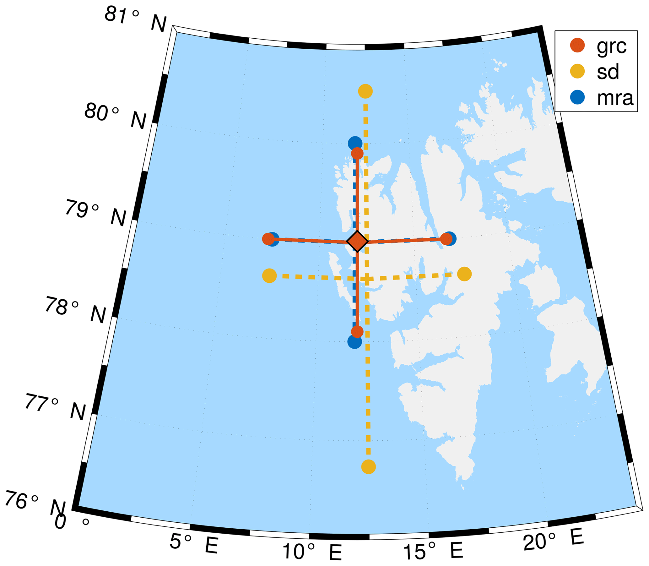
Figure 1 Location of the data points of GROMOS-C, MERRA-2 and SD-WACCM at 3 hPa (37 km) which are used to calculate the ozone gradient above Ny-Ålesund (indicated with a red square).

2.1.2 GROMOS-C wind measurements

From the ozone spectra measured in the four cardinal directions we retrieve daily mean zonal and meridional wind profiles with the same method as described in Hagen et al. (2018). Figures 2 and 3 show the time series of zonal and meridional wind speeds retrieved from the GROMOS-C spectra. The grey horizontal lines in Figs. 2a and 3a indicate the upper and lower bounds of a measurement response of 0.5 which we define as the trustworthy altitude range of the measurement. The measurement response is defined as the area below the averaging kernel of a given altitude and indicates the sensitivity of the retrieval (Rodgers, 2000). For wind retrievals the a priori profile is 0 m s⁻¹ to allow positive and negative wind speeds with the same probability. This is especially important for the observation of sudden wind reversals in the context of extreme events. The grey background indicates data gaps or days where the retrieval did not converge because of too high noise levels when the opacity of the troposphere was high or when the measurement response was smaller than 0.5 for the whole profile.

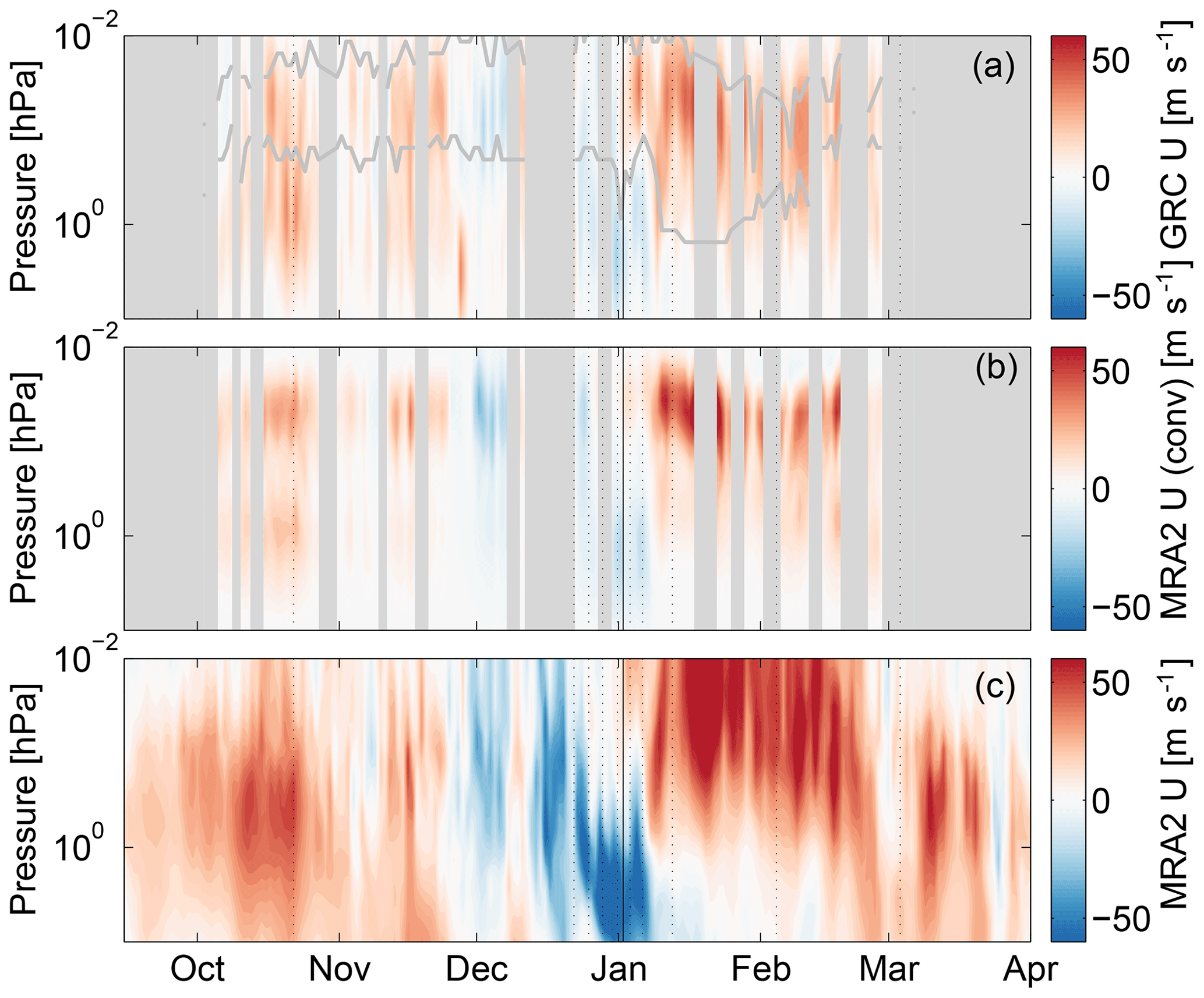
Figure 2 Zonal wind at Ny-Ålesund measured with GROMOS-C (a) and from the MERRA-2 reanalysis convolved with the averaging kernels of GROMOS-C (b) and unconvolved (c) for winter 2018/2019. The grey background indicates data gaps and the grey lines indicate the area where the measurement response is larger than 0.5. The dotted lines indicate the dates of the polar vortex snapshots in Fig. 6 and the solid line shows the central date of the SSW.

Figure 3 Same as in Fig. 2 but for meridional wind.

Compared to the microwave radiometers (WIRA, Rüfenacht et al., 2012, and WIRA-C, Hagen et al., 2018), which were specifically designed for wind measurements, GROMOS-C has a lower measurement response and the wind profiles cover a smaller altitude range. This is because they measure the ozone line at a higher frequency (142 GHz) where the Doppler shift is larger, the instrument noise temperature is lower and the used spectrometers have a higher spectral resolution.

The comparison of zonal and meridional wind measurements with convolved MERRA-2 data shows a good agreement (Figs. 2 and 3). Several wind reversals in the mesosphere from November to January are captured. Even in the stratosphere, where the measurement response is below 0.5, the westward wind in the beginning of January and the predominantly eastward winds in October and November are captured as well as the strong northward wind components before and after the SSW.

2.2 MIAWARA-C

MIAWARA-C (MIddle Atmospheric WAter vapour RAdiometer for Campaigns) is a ground-based microwave radiometer which measures the pressure-broadened rotational emission line of water vapour at 22 GHz. The instrument has an uncooled heterodyne receiver system and an FFT spectrometer with 400 MHz bandwidth and a spectral resolution of 30.5 kHz. The system noise temperature of MIAWARA-C is about 150 K. From the measured spectra we retrieve water vapour profiles with QPACK (Eriksson et al., 2005) and ARTS2 (Eriksson et al., 2011), using an optimal estimation method (Rodgers, 1976). The profiles cover an altitude range of 37–75 km with a time resolution of 2–4 h, depending on the opacity of the troposphere. A detailed description of the instrument and the retrieval algorithm is given in Straub et al. (2010) and Tschanz et al. (2013).

MIAWARA-C was located at Sodankylä and Bern in the years 2010–2013 and has been located at Ny-Ålesund since September 2015. At Bern and Sodankylä an offset of +13 % compared to satellite measurements was seen in the mesosphere, but in the upper stratosphere the measurements agreed mostly within ±5 % (Tschanz et al., 2013). A comparison at Ny-Ålesund with EOS-MLS over 3 years shows an average offset over the full altitude range of 10 %–15 %, depending on altitude but constant in time. The median relative difference of MIAWARA-C measurements to SD-WACCM simulations and measurements from the ACE-FTS satellite instrument is within ±5 % on average (Schranz et al., 2019).

2.3 EOS-MLS

EOS-MLS is the Earth Observing System Microwave Limb Sounder onboard NASA's Aura satellite (Waters et al., 2006). It was launched in 2004 into a sun-synchronous orbit with 98^∘ inclination and a period of 98.8 min. At Ny-Ålesund it passes twice a day at about 04:00 and 10:00 UT. We use the version 4.2 temperature product (Schwartz et al., 2015). The temperature profiles are derived from the 118 and 240 GHz radiometers and cover an altitude range from 10 to 90 km.

2.4 SD-WACCM

SD-WACCM (Brakebusch et al., 2013) is the specified dynamics version of NCAR's Whole Atmosphere Community Climate Model (WACCM, Marsh et al., 2013) and the atmospheric component of the Community Earth System Model (CESM). The model grid extends from ground to 145 km altitude using 88 levels with a vertical resolution of 0.5–4 km. The spatial resolution is 1.9^∘ latitude × 2.5^∘ longitude and the temporal resolution is 30 min. In SD-WACCM the dynamics is constrained by meteorological analysis fields from GEOS5 (Rienecker et al., 2008). This means that at every model time step horizontal winds, temperature, surface wind stress, surface pressure and specific and latent heat flux are nudged towards the analysis fields in order to keep a realistic representation of the dynamics. The nudging strength is 10 %, and it is performed up to an altitude of 70 km with a transition from 10 % to 0 % nudging between 70 and 75 km. The chemistry module is based on MOZART the model for ozone and related chemical tracers (Emmons et al., 2010). The ozone variability in the Arctic middle atmosphere related to photochemical reactions is represented realistically (Schranz et al., 2018).

A previous comparison with GROMOS-C and MIAWARA-C at Ny-Ålesund over 3 years between 2015 and 2018 showed a median relative difference of 5 % up to 0.7 hPa for ozone, and for water vapour it is within ±5 % up to 0.1 hPa (Schranz et al., 2019).

2.5 MERRA-2

The Modern-Era Retrospective Analysis for Research and Applications, version 2 (MERRA-2, Gelaro et al., 2017) is the latest atmospheric reanalysis from NASA's GMAO (2015). It is calculated on a cubed-sphere grid with a resolution of $\mathrm{0.5}{}^{\circ }\times \mathrm{0.625}{}^{\circ }$ and spans from the surface up to 0.01 hPa using 72 vertical levels. Measurements are assimilated in a 3D-Var assimilation scheme. Temperature and ozone profile measurements from EOS-MLS are used to also assimilate data in the upper stratosphere and mesosphere. EOS-MLS temperature profiles are assimilated above 5 hPa and ozone profiles at 215–0.02 hPa. For the period when primarily EOS-MLS data were assimilated in the reanalysis (2003–2012), a comparison with MIPAS measurements was performed. It shows that MERRA-2 underestimates ozone VMRs by up to 5 % compared to MIPAS during winter (DJF) in the Arctic stratosphere (100–1 hPa) (Wargan et al., 2017).

3 Characteristics of the SSW in winter 2018/2019

During winter 2018/2019 a major SSW took place. It was first discussed by Rao et al. (2019), and they stated that the SSW is neither a typical displacement nor a typical split event. According to the zonal mean zonal wind data from MERRA-2, the central date of the SSW is 2 January 2019. It is defined as the first day when the zonal mean zonal wind reverses from eastward to westward at 60^∘ N and 10 hPa (Charlton and Polvani, 2007). In this section we give an overview of the meteorological background situation and discuss the observations at Ny-Ålesund in a global context.

3.1 Meteorological background situation

An overview of the zonal mean temperatures measured with EOS-MLS and zonal mean zonal wind from MERRA-2 at 10 hPa in the stratosphere (Fig. 4) and at 0.1 hPa in the mesosphere (Fig. 5) for winter 2018/2019 reveals the signatures of the SSW. At 10 hPa the latitudinal temperature gradient from 60 to 90^∘ N reversed on 25 December and stayed reversed for 1 month. At 80^∘ N the zonal mean temperature increased by about 45 K in less than a week. The reversal of the latitudinal temperature gradient at 10 hPa was accompanied by a reversal of the zonal mean zonal wind between 60 and 90^∘ N which classifies the warming event as a major sudden stratospheric warming according to the definition of McInturff (1978). The zonal mean zonal wind also stayed reversed for about 1 month. In the stratosphere the polar vortex recovered in February and stayed undisturbed until the end of March. In the mesosphere at 0.1 hPa the zonal mean temperature dropped by about 35 K at 80^∘ N. The wind reversed for about a week at 60^∘ N and for about 2.5 weeks at 80^∘ N. Already in mid January the polar vortex recovered in the mesosphere and gained high wind speeds.

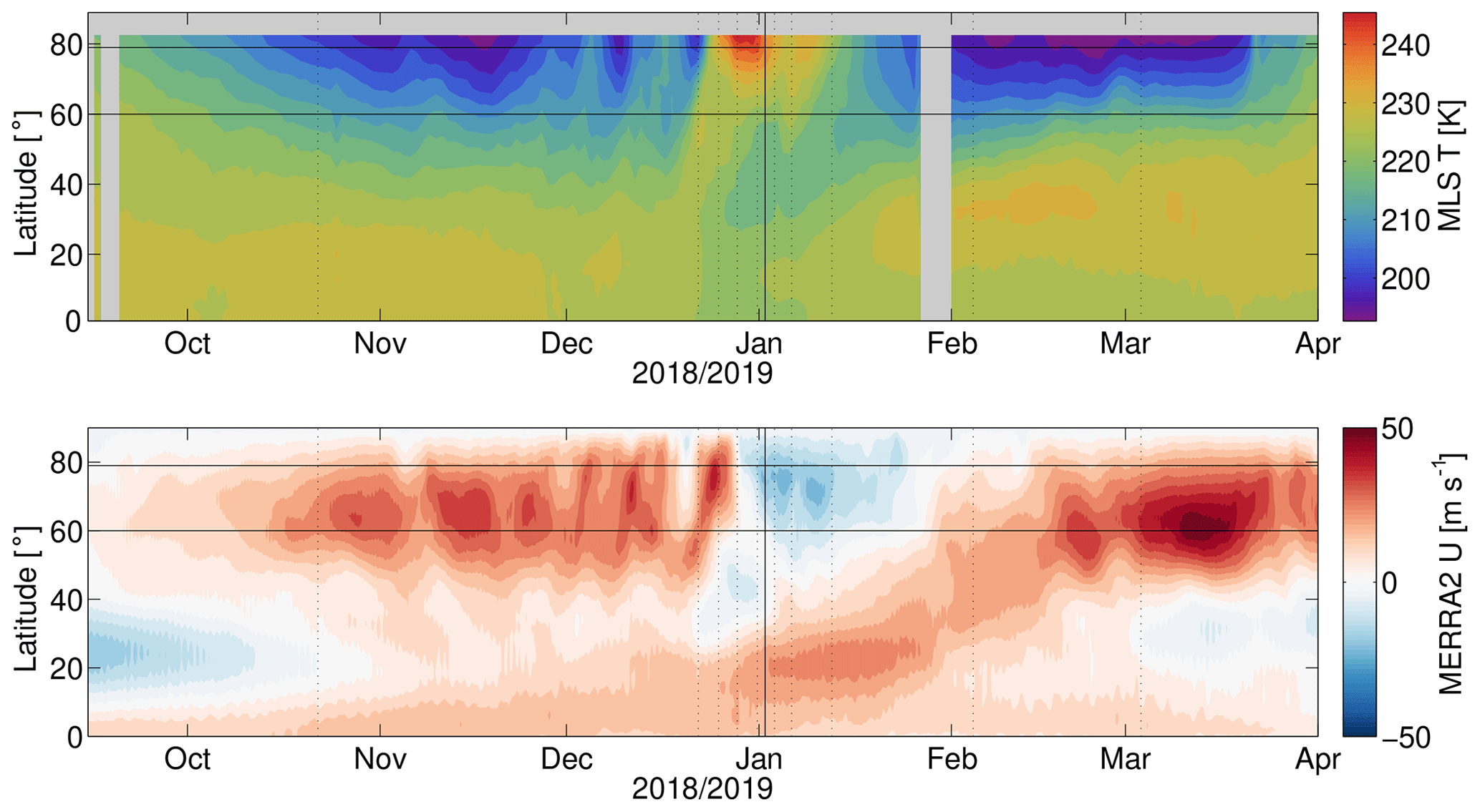
Figure 4 Zonal mean temperature from MLS and zonal mean zonal wind from MERRA-2 at 10 hPa in the stratosphere for winter 2018/2019. The dotted lines indicate the dates of the polar vortex snapshots in Fig. 6 and the solid line shows the central date of the SSW. The horizontal lines indicate 60 and 79^∘ N.

Figure 5 Same as in Fig. 4 but at 0.1 hPa in the mesosphere.

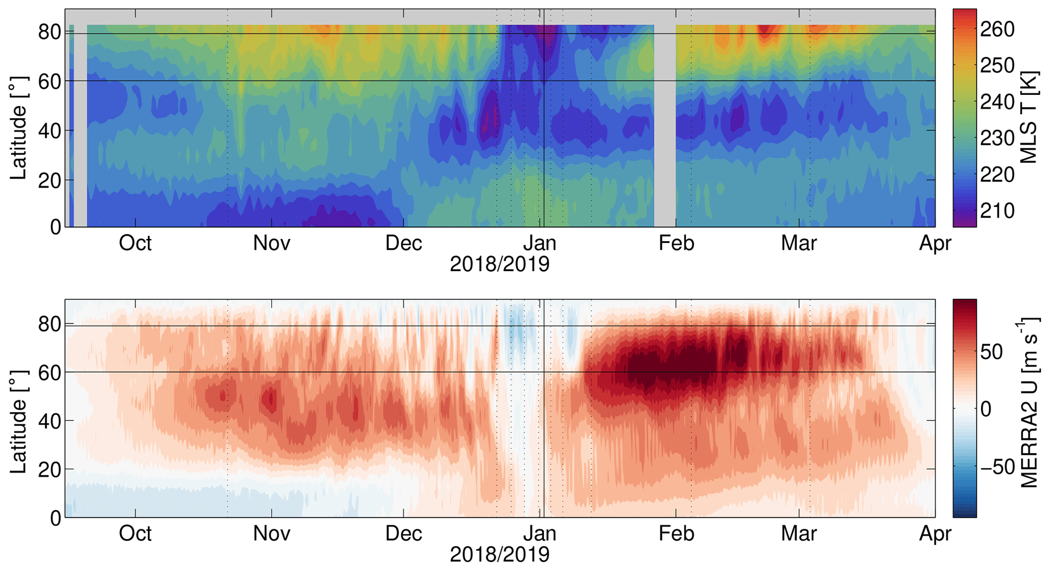
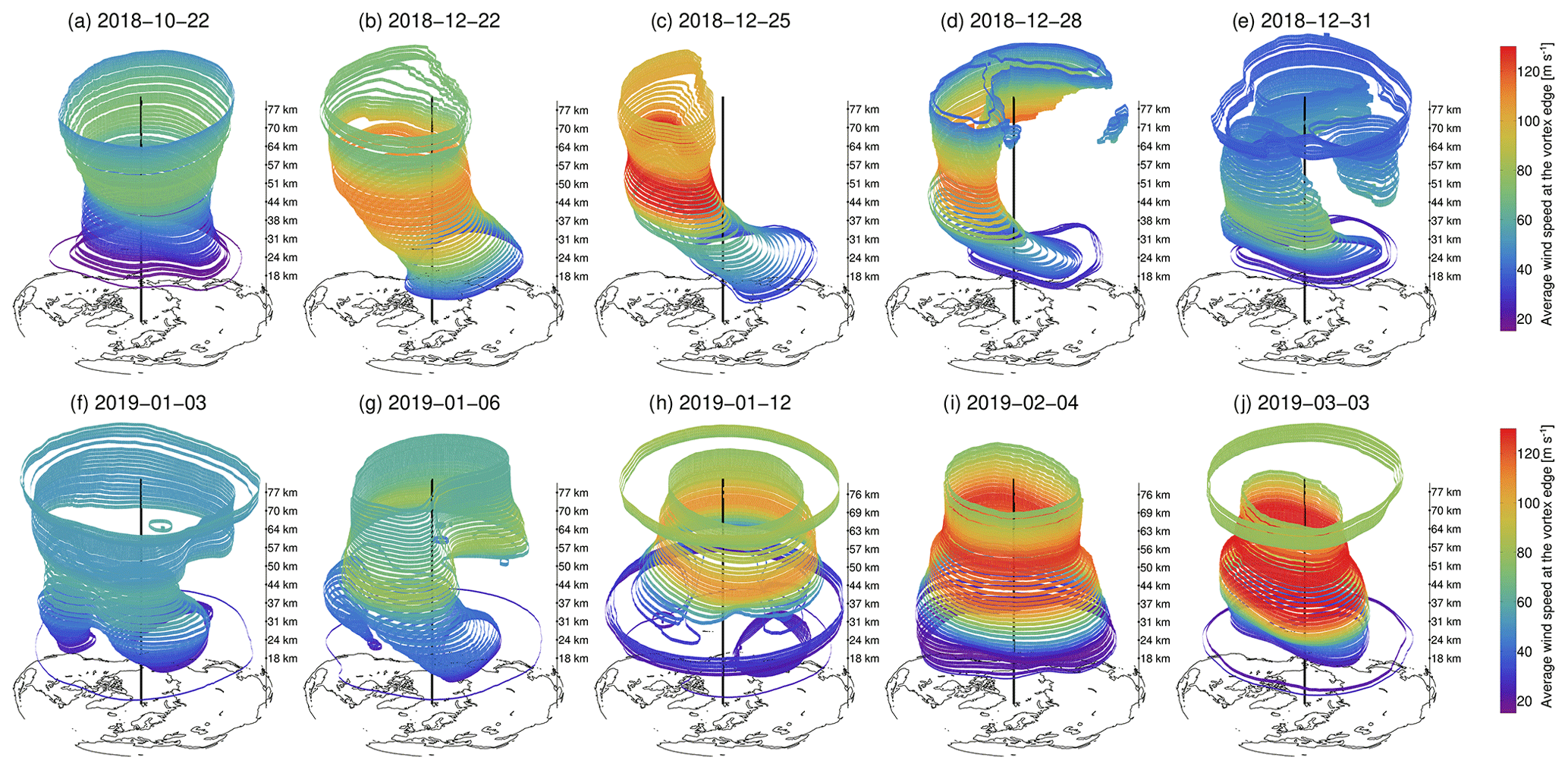
Figure 6 Contours of the polar vortex during winter 2018/2019. The central date of the SSW is 2 January 2019. The vertical black line is positioned at Ny-Ålesund.

The evolution of the polar vortex during the SSW of winter 2018/2019 is visualized in Fig. 6. For a given pressure level the polar vortex is determined as the geopotential height (GPH) contour north of 15^∘ N with the highest absolute wind speed compared to other GPH contours at the same pressure level. The GPH and wind data are taken from ECMWF and the method is discussed in detail in Scheiben et al. (2012). For altitudes below 10 hPa (about 30 km) the SSW was already discussed in Rao et al. (2019, 2020). In the middle atmosphere the vortex started to shift notably around 20 December. It was shifted towards Greenland in the mesosphere, whereas the stratospheric part was shifted towards Siberia. In the mesosphere the polar vortex started to be torn apart towards the end of December and split in three sub-vortices on 31 December. In the stratosphere it eventually split on 3 January, which is shortly after the central date of the SSW. At the same time in the mesosphere, the polar vortex already regained a circular shape and the wind speed started to increase. On 12 January the polar vortex was reestablished in the mesosphere, whereas in the stratosphere wind speeds are still very low and the algorithm detected the polar vortex edge at a latitude of 20^∘ N, which indicates a complete breakdown of the polar vortex system after the SSW in the stratosphere.

3.2 Observations at Ny-Ålesund

At Ny-Ålesund we were measuring ozone, water vapour and zonal and meridional wind profiles in the middle atmosphere with our ground-based microwave radiometers. The SSW during winter 2018/2019 was clearly visible in our data from Ny-Ålesund. Temperature measurements from EOS-MLS at Ny-Ålesund (Fig. 7, top) show that within 1 week stratospheric (10 hPa) temperatures increased by 50 K and the stratopause descended from about 0.15 to 1.5 hPa. The temperature in the mesosphere (0.1 hPa) decreased by 50 K. After the SSW the stratopause was first indistinct and then re-formed at a much higher altitude around 0.02 hPa. The stratopause height was then gradually decreasing until it reached about 1 hPa at the end of March. The elevated stratopause is a phenomenon which can occur after an SSW and has been previously observed (e.g. Manney et al., 2008). In a model climatology Chandran et al. (2013) found that 68 % of the SSWs with elevated stratopause are split-type events and that the remaining 32 % are displacement events. Matthias et al. (2012) compiled a composite of SSW events with an elevated stratopause between 1998 and 2011 using ECMWF data and MF-radar observations revealing the formation of an elevated stratopause in the mesospheric wind as strong zonal wind enhancement after the SSW. Later, Limpasuvan et al. (2016) made a composite analysis of SSWs with an elevated stratopause using WACCM data and explained the occurrence of an elevated stratopause with strong, wave-induced downwelling in the mesosphere which leads to adiabatic warming.

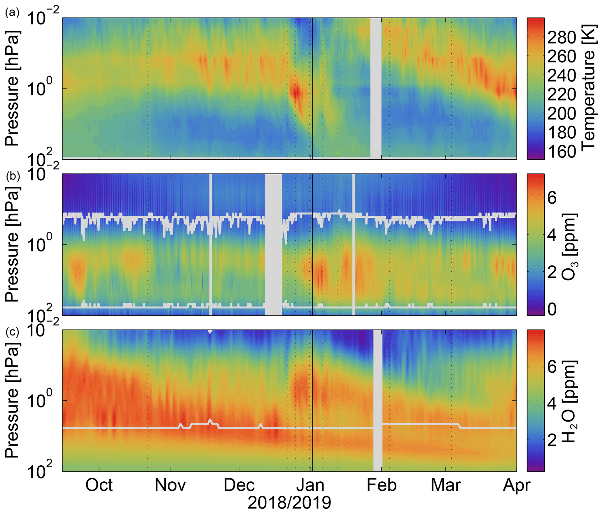
Figure 7 EOS-MLS temperature (a), GROMOS-C ozone VMR (b) and MIAWARA-C water vapour VMR (c) time series at Ny-Ålesund for winter 2018/2019. The dotted lines indicate the dates of the polar vortex snapshots in Fig. 6 and the solid line shows the central date of the SSW. The grey background indicates data gaps and the grey lines indicate the upper and lower bounds of the area where the measurement response is larger than 0.8 for GROMOS-C and the lower bound of this area for MIAWARA-C.

The zonal and meridional winds at Ny-Ålesund were retrieved from the GROMOS-C ozone spectra and compared to convolved and unconvolved MERRA-2 data (Figs. 2 and 3). The zonal wind was predominantly eastward in October and November. In the beginning of December it reversed to a westward direction. Except for a few days in mid December, it stayed westward for the whole month in the stratosphere and lower mesosphere. At the time of the stratospheric vortex split (Fig. 6f) we see strong westward winds in the stratosphere, whereas in the mesosphere the wind already reversed to an eastward direction. After the SSW a strong and stable vortex reestablishes in the mesosphere where higher wind speeds are measured than before the SSW, which is in agreement with MF-radar observations at Andenes, Norway (69^∘ N) (Matthias et al., 2012). The wind speeds in the stratosphere stay low until the polar vortex starts to recover in mid February.

The meridional wind speeds in autumn are low compared to the zonal wind speed because the polar winter cyclone which dominates the dynamics in the Arctic is centred at the pole (Fig. 6a). When the vortex shifted away from Ny-Ålesund towards Greenland and Canada at the end of December (Fig. 6d), very strong northward wind components were measured from the mesosphere down to the stratosphere. Shortly after the central date of the SSW, the stratospheric vortex split and meridional wind speeds were low. When the edge of the newly formed vortex was above Ny-Ålesund (Fig. 6g), this led to a very strong northward wind component for a second time. This was followed by southward winds in mid January because the polar vortex was slightly shifted towards Siberia. From mid January on the meridional wind speeds are similar to the autumn period.

Figure 7 (middle) presents the ozone VMR time series measured with GROMOS-C in the eastward direction. The ozone layer is clearly visible and the maximum of the ozone VMR is at about 3 hPa (37 km). During the SSW the ozone VMR increased in the upper and middle stratosphere and reached up to 6.5 ppm. Except for a short ozone decrease in the upper stratosphere around 12 January, the ozone VMR stays visibly enhanced compared to November until the end of February. In October and February/March a prominent diurnal cycle is present in the mesosphere. Signatures of wave activity are found during November and again in March, with the largest amplitudes around 2 hPa. Using a wavelet-like approach which is described in Hocke and Kämpfer (2008) and Hocke (2009), we find peak-to-peak amplitudes of 0.8 ppm and periods of 3–4 d in November. In March we find peak-to-peak amplitudes of 1 ppm and periods of 1.5–2.5 d. The wave activity in November is also seen in the water vapour time series.

The water vapour measurements from MIAWARA-C are shown in Fig. 7 (bottom). In autumn the water vapour is descending inside the polar vortex. For the period of 15 September–1 November 2018 the effective descent rate of water vapour calculated from the 5.5 ppm isopleth is 360 m d⁻¹. This is slightly lower than in the years 2015–2017, when the average effective descent rate was 433 m d⁻¹ (Schranz et al., 2019). During the SSW we observe a sudden increase of 2.5 ppm around 0.3 hPa, whereas at the same time in the stratosphere at 3 hPa the water vapour VMR dropped by 1 ppm. After the SSW the mesospheric vortex reestablishes and we find again a vertical descent of the mesospheric water vapour.

3.3 O₃ and H₂O measurements in a global context

To show the local ozone and water vapour measurements from our microwave radiometers in a global context, we use Northern Hemisphere ozone and water vapour data from the SD-WACCM model and indicate the contour of the polar vortex in Figs. 8 and 9.

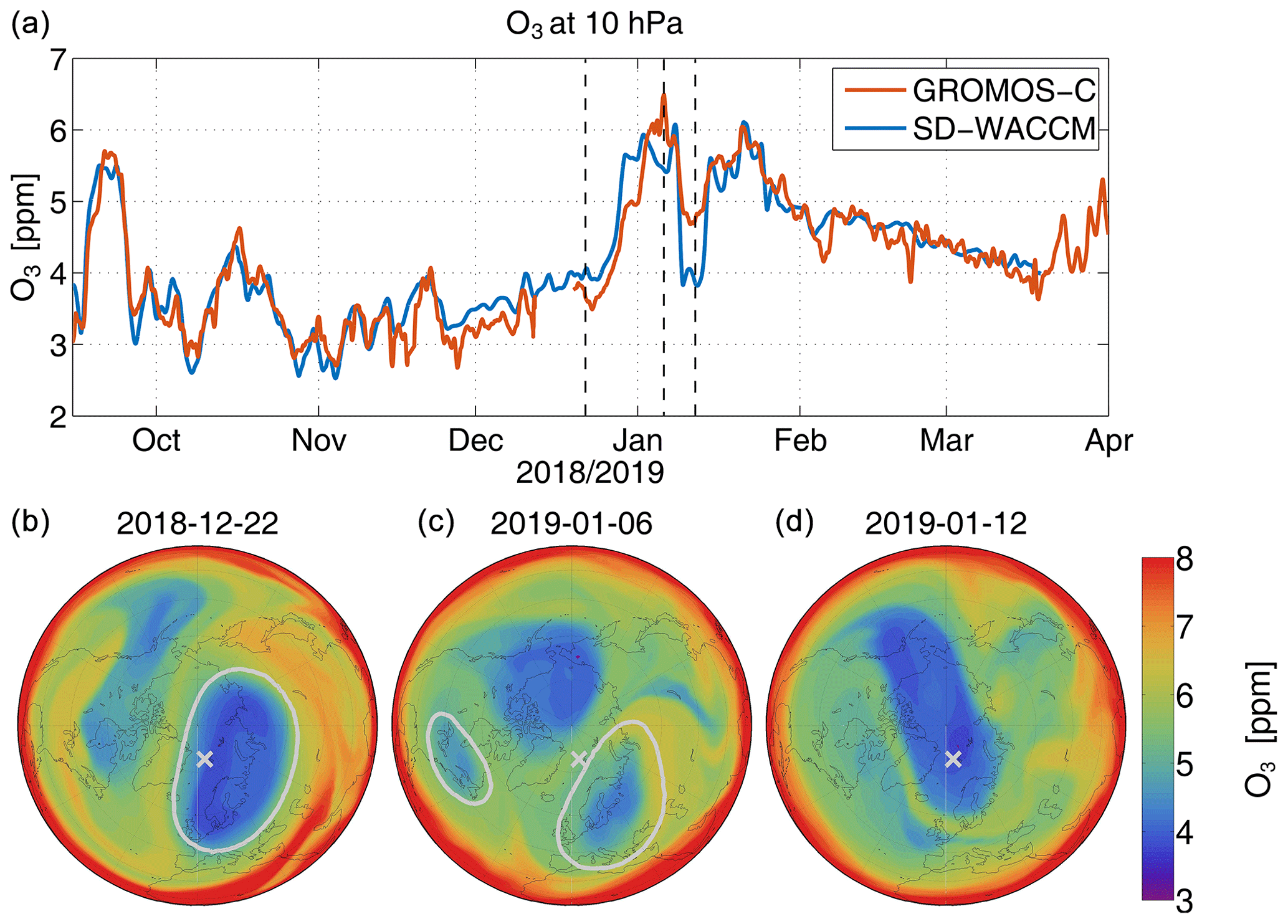
Figure 8 GROMOS-C and SD-WACCM ozone VMR time series at 10 hPa smoothed by a 1 d running mean (a) and SD-WACCM ozone VMR at 10 hPa in the Northern Hemisphere (b–d) for three dates which are indicated with dashed lines in panel (a). In the NH plots (b–d) the location of Ny-Ålesund and the polar vortex edge are indicated in grey.

Figure 9 Same as in Fig. 8 but for MIAWARA-C water vapour VMR time series at 0.3 hPa.

For ozone we chose an altitude of 10 hPa, which lies within the main ozone VMR layer in the stratosphere (Fig. 8). Prior to the SSW in November and December, Ny-Ålesund was inside of the polar vortex and the ozone VMR was about 2.5–4 ppm. After the central date when the polar vortex split and was shifted away from Ny-Ålesund, ozone VMR reached 6.5 ppm. At the same time the Aleutian anticyclone is moving to the pole and the absence of sunlight leads to a low-ozone pocket inside of the anticyclonic wind system at about 10 hPa. This effect was observed by Manney et al. (1995) and explained by Morris et al. (1998) and Nair et al. (1998): the air inside of the Aleutian anticyclone is dynamically isolated at high latitudes long enough such that the ozone VMR decreases and approaches the local photochemical equilibrium. These low-ozone pockets were previously observed at Thule, Greenland, with ground-based microwave radiometers and a correlation between the ozone VMR and the solar exposure time of the air parcel within the last 10 d was found (Muscari et al., 2007). The polar vortex completely breaks down at this altitude after the split and the elongated Aleutian anticyclone passes over Ny-Ålesund, where the ozone VMR drops to 4.7 ppm above 15 hPa for 5 d. Below 15 hPa, where ozone lifetimes are longer, no ozone decrease is seen. The ozone VMR then continuously decreases until it reaches a minimum of 3.6 ppm in mid March. The ozone VMR of SD-WACCM in the polar plots differs from the GROMOS-C measurements (e.g. inside of the Aleutian high the SD-WACCM ozone VMRs are lower than for GROMOS-C) because of the difference in the altitude resolution of the two datasets. In the upper stratospheric water vapour measurements we see that the overpass of the Aleutian anticyclone does not affect the water vapour VMR.

For water vapour we show the MIAWARA-C measurements in a global context at 0.3 hPa in the mesosphere in Fig. 9. Prior to the SSW Ny-Ålesund was inside of the polar vortex. Shortly before the central date of the SSW, the polar vortex moved away from Ny-Ålesund and the water vapour VMR increased by 2.5 ppm within 4 d. The vortex regains its circular shape soon and water vapour is descending, leading to a decrease in VMR at 0.3 hPa and to a growing water vapour gradient across the vortex edge. The minimum VMR is reached in mid February, and in March air masses are again rising inside of the summer anticyclone and VMRs increase. SD-WACCM captures the water vapour variation at 0.3 hPa nicely during the SSW. It however reaches the minimum VMR already at the beginning of February.

Since September 2015, when GROMOS-C and MIAWARA-C were installed at Ny-Ålesund, three major SSWs have taken place in the Northern Hemisphere. The major final warming of March 2016 and the major SSW of February 2018 were discussed in Schranz et al. (2019). The evolution of ozone and water vapour above Ny-Ålesund during the SSW of winter 2018/2019 and the stratospheric final warming of March 2016 were similar. Both SSWs led to stratospheric ozone increases when the polar vortex moved away from Ny-Ålesund and an ozone decrease above 15 hPa when a low ozone pocket inside of the Aleutian anticyclone passed Ny-Ålesund. In February 2018 ozone VMRs doubled when the polar vortex split. Increases in mesospheric water vapour were observed during all three SSWs. A pronounced elevated stratopause only developed after the SSW in winter 2018/2019.

4 Small-scale spatial variability of O₃

GROMOS-C measures ozone spectra in the four cardinal directions under an observation angle of 22^∘ and a time resolution of 2 h (see Sect. 2.1.1). From these spectra, four separate ozone profiles are retrieved along the lines of sight. At an altitude of 3 hPa (37 km) the distance between the E–W and N–S measurement locations is 184 km. We use the measurements at these four locations to calculate daily mean horizontal ozone gradients above Ny-Ålesund. For intercomparison we also used ozone data from the SD-WACCM model and the MERRA-2 reanalysis. Figure 1 shows the measurement locations of GROMOS-C at 3 hPa and the grid points of SD-WACCM and MERRA-2. The ozone profiles of SD-WACCM and MERRA-2 were convolved with the averaging kernel of GROMOS-C before the gradients were calculated.

4.1 Ozone gradients at Ny-Ålesund

Figure 10 shows magnitude and angle of the daily mean horizontal ozone gradients above Ny-Ålesund over the course of winter 2018/2019 and at an altitude of 3 hPa. An angle of φ=0^∘ indicates an eastward-pointing gradient, meaning that ozone VMRs are increasing towards the east. An angle of $\mathit{\phi }=+\mathrm{90}$^∘ indicates a northward-pointing gradient. The gradients from the GROMOS-C data show a clear seasonal variation. In October ozone is increasing towards lower latitudes with on average 0.2 ppm / 184 km. During November the gradients start to point to higher latitudes occasionally, and in December they mainly reversed and indicate higher ozone VMR at higher latitudes. From December on the ozone gradients predominantly point northwards to eastwards until mid February, when the gradients suddenly turn southward and the magnitude increases and reaches up to 0.8 ppm / 184 km. During the SSW the gradients first point in northeastern directions and then in northwestern directions. This is followed by strong eastward-pointing gradients in the end of January. During the first half of February the gradients are again mostly pointing towards higher latitudes and are with a magnitude of 0.1 ppm / 184 km smaller than the average magnitude of 0.2 ppm / 184 km. The magnitude relative to the mean ozone VMR of the four cardinal directions is 4 % / 184 km on average.

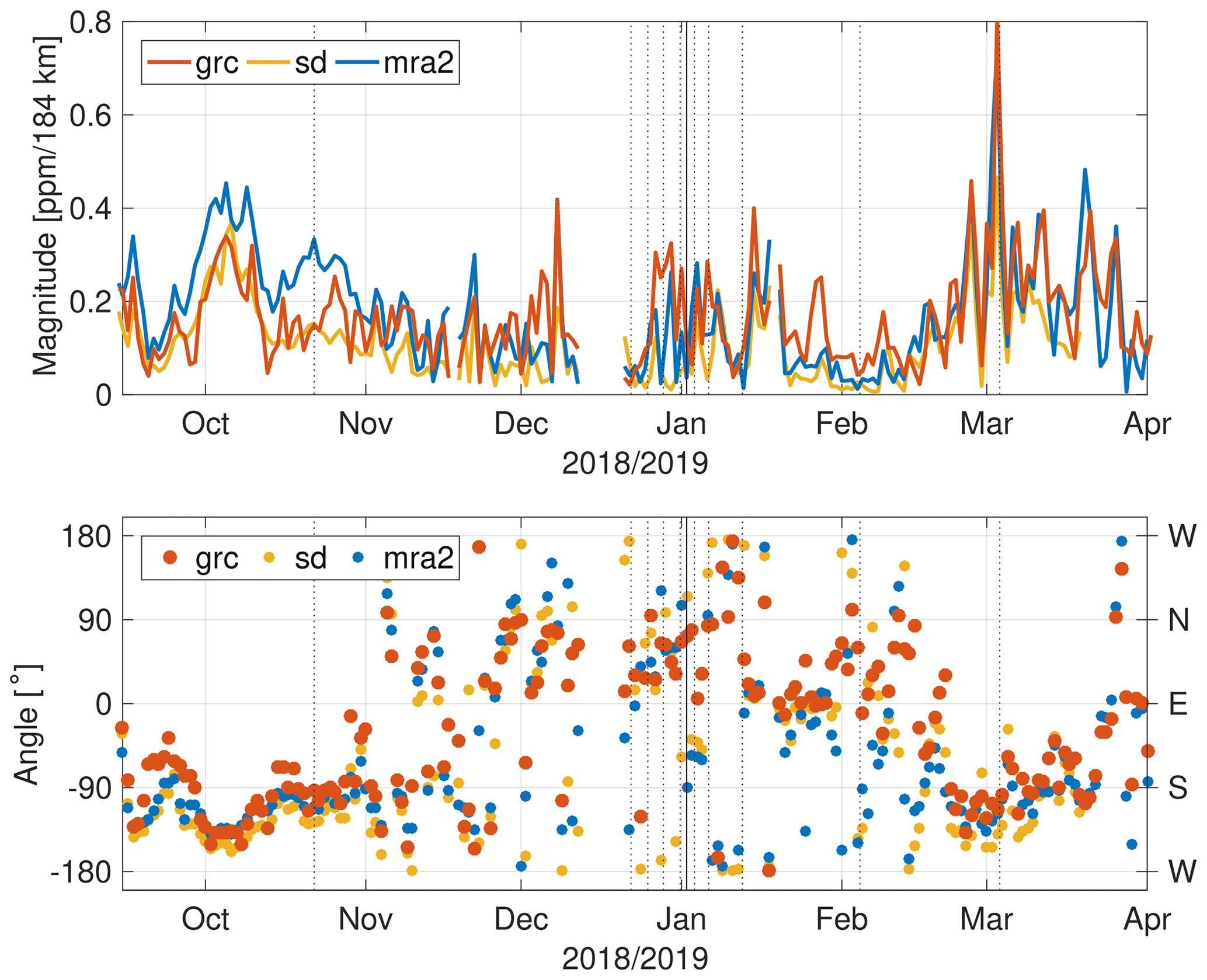
Figure 10 Magnitude and angle of the ozone gradients at 3 hPa above Ny-Ålesund from GROMOS-C, SD-WACCM and MERRA-2 data during winter 2018/2019. The dotted lines indicate the dates of the polar vortex snapshots in Fig. 6 and the solid line shows the central date of the SSW. The cardinal directions which correspond to an angle are indicated on the right.

The general pattern of the ozone gradients at 3 hPa has already been seen in the 3 previous years of GROMOS-C observations at Ny-Ålesund. The mean over every day of the year of the north–south gradients from 4 years of GROMOS-C measurements shows that the gradients at 3 hPa are mainly pointing to lower latitudes from September until the beginning of November and then again during March. During summer and winter the gradients point mainly towards higher latitudes. This seasonal pattern is observed in the upper stratosphere at altitudes between about 10 and 1 hPa.

Sparling et al. (2006) analysed the small-scale variability of ozone from measurements with a UV absorption instrument mounted on an aircraft. At 18–21 km altitude and inside of the NH polar vortex they found average relative differences of 4 % across a scale of 100 km. Differences in the magnitudes of N–S and E–W gradients were not found at this altitude and at latitudes >30^∘ in winter. For GROMOS-C at 20 km altitude the distance between the N–S and E–W measurement locations is 100 km. In the period where Ny-Ålesund was located inside of the polar vortex (October–March, except January) we find magnitudes of 0.1 ppm / 100 km on average, which corresponds to a relative difference of 4 % and is in exact agreement with the measurements of Sparling et al. (2006).

4.2 Comparison with SD-WACCM and MERRA-2

We compared the evolution of the horizontal ozone gradients at 3 hPa, measured by GROMOS-C with MERRA-2 and SD-WACCM (Fig. 10). The comparison shows that the reanalysis and the model capture the prominent features of the magnitude time series, for example the low magnitudes in the beginning of February and the subsequent variability in March. On average the magnitude of the SD-WACCM gradients is 28 % lower, and MERRA-2 is 11 % higher than GROMOS-C. The correlation coefficient with GROMOS-C is 0.7 for both SD-WACCM and MERRA-2. We use Pearson's correlation coefficient, which is defined as the covariance of the two datasets divided by the product of the standard deviations of the two datasets: $\mathit{\rho }=\mathrm{cov}(A,B)/\left({\mathit{\sigma }}_A{\mathit{\sigma }}_B\right)$. In October MERRA-2 shows about 0.11 ppm / 184 km (about 60 %) higher magnitudes, while the angles are still captured well. The angles agree again well in the end of January when the gradients were eastward pointing and then again in the end of February and during March. From November until the end of February the angles are less stable, but in December and January they are mainly >0 for GROMOS-C, whereas SD-WACCM and MERRA-2 also show negative angles. During October and March the angles of SD-WACCM and MERRA-2 are on average smaller than the angles of GROMOS-C by 22 and 10^∘ respectively.

4.3 Influence of planetary waves on local ozone gradients

The horizontal ozone gradients measured by GROMOS-C show strong variations throughout the observation period. Eixmann et al. (2020) investigated the temporal variability of the stratopause region temperatures using nightly averaged lidar and reanalysis data and found that the day-to-day variability was mostly driven by stationary planetary waves 1, 2 and 3. Large amplification of the planetary wave amplitude was observed prior to and during SSWs (e.g. Lawrence and Manney, 2020; Matthias and Ern, 2018). To characterize the influence of the planetary waves on the variability of the ozone gradients, we calculated amplitude and phase of the stationary planetary waves in the MERRA-2 zonal and meridional wind fields using the wave diagnostics algorithm described in Baumgarten and Stober (2019). We first present the evolution of the stationary planetary waves and discuss the dominant gradient patterns throughout winter 2018/2019 in the context of the planetary wave activity. We further demonstrate the influence of stationary planetary waves 1 and 2 on the ozone gradients by means of reconstructing local wind fields from the planetary waves.

Figure 11 shows amplitude and phase of the stationary planetary waves 1 and 2 in the zonal wind field of MERRA-2 at 79^∘ N and 3 hPa. Waves with higher wave numbers have low amplitudes and are not considered here. The amplitudes of waves 1 and 2 start to increase in November and reach 60 and 25 m s⁻¹ respectively with a stable phase. The amplitude of wave 2 already decreases in mid December, whereas wave 1 is stable during December and shows a period of about 10 d. At the end of December wave 1 breaks down and the SSW takes place. After the SSW the wave amplitudes stay below 20 m s⁻¹ until mid March.

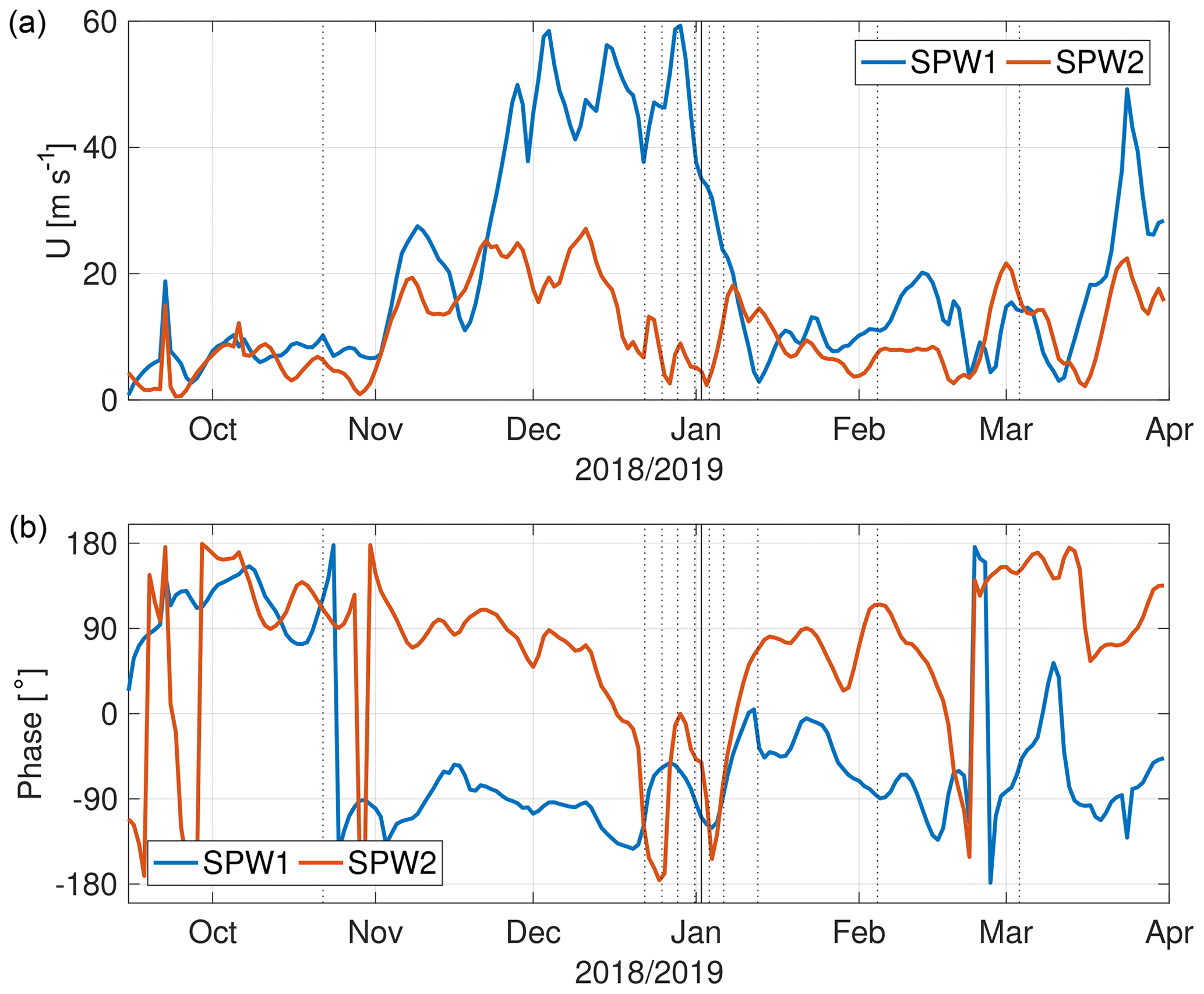
Figure 11 Amplitude (a) and phase (b) of the stationary planetary waves 1 and 2 calculated from the MERRA-2 zonal wind. The dotted lines indicate the dates of the polar vortex snapshots in Fig. 6 and the solid line shows the central date of the SSW.

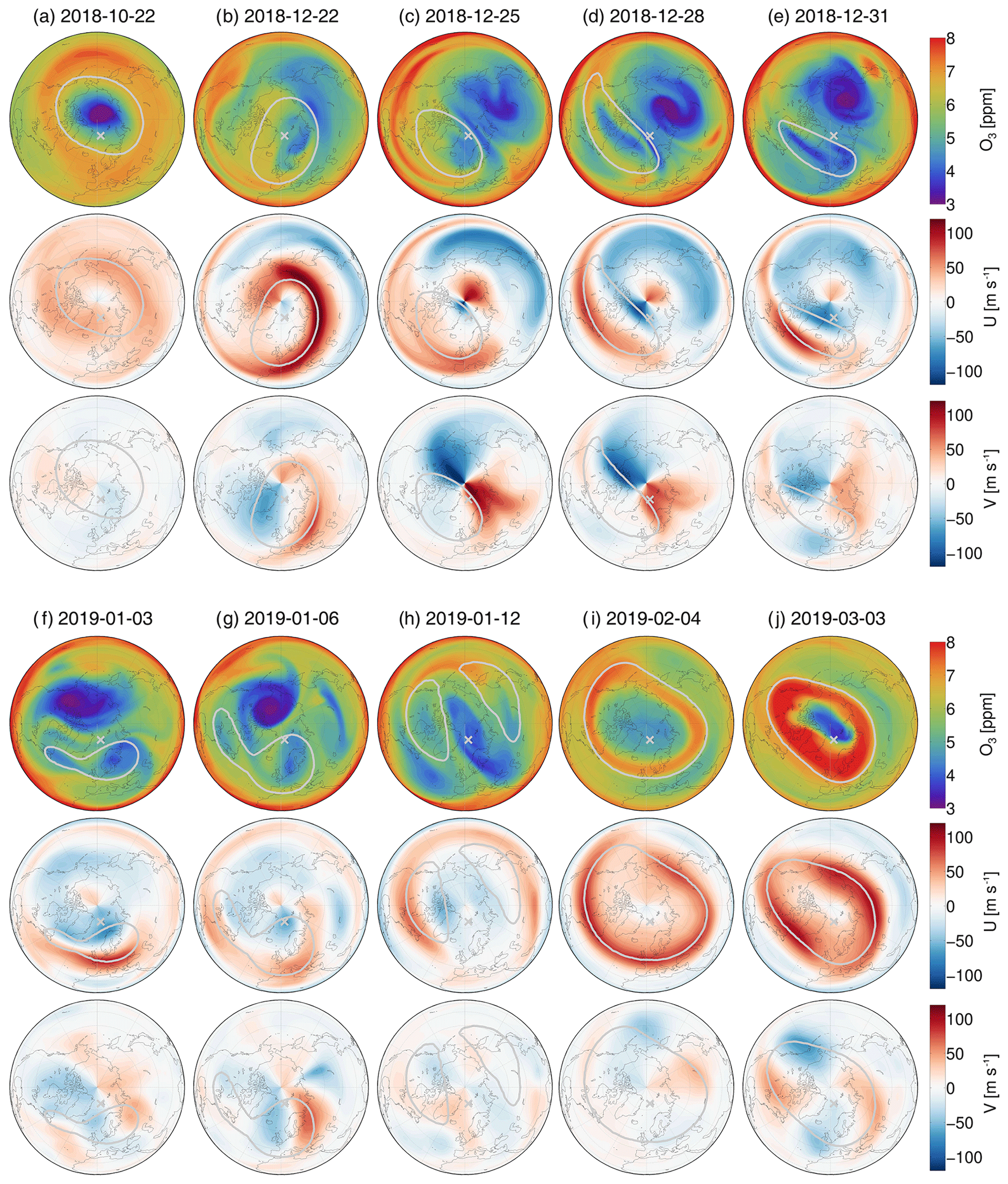
Figure 12 SD-WACCM ozone VMR, zonal wind and meridional wind at 3 hPa. The edge of the polar vortex and the location of Ny-Ålesund are indicated in grey. The dates correspond to the polar vortex snapshots in Fig. 6.

Figure 12 shows SD-WACCM ozone at 3 hPa in the Northern Hemisphere, illustrating the different gradient patterns observed throughout winter 2018/2019 at Ny-Ålesund. The dates correspond to the polar vortex snapshots in Fig. 6. Additionally, the zonal and meridional wind components from SD-WACCM are shown for the same dates, and the contour of the polar vortex is indicated.

We use amplitude and phase of the planetary wave in Fig. 11 and the ozone and wind plots in Fig. 12 to discuss the different gradient patterns observed with GROMOS-C at Ny-Ålesund throughout the winter (see Fig.10). In October the amplitudes of the planetary waves 1 and 2 are low and the polar vortex is mainly centred at the pole and the zonal wind field is zonally symmetric (Fig. 12a), which leads to a transport barrier between midlatitude and polar air (see e.g. Meek et al., 2017; Manney et al., 1994). At the latitude of Ny-Ålesund and at 3 hPa there is no net chemical ozone production during the winter season (October–mid March), which leads to a stable southward-pointing ozone gradient. The net chemical ozone production is the difference between the chemical ozone production and loss rate from SD-WACCM (not shown). In November the amplitudes of waves 1 and 2 start to increase and the polar vortex is shifted towards Asia or Europe, which leads to enhanced meridional transport and reverses the direction of the ozone gradients at Ny-Ålesund. The increasing wave activity reduces the latitudinal mixing barrier and the average magnitude of the ozone gradients decreases compared to October. During the SSW Fig. 12b–g) shows the inflow of midlatitude air into the polar region and filamentary structures in the ozone field lead to variations in the magnitude and angle of the ozone gradients. In mid January a low ozone pocket crosses Ny-Ålesund (Fig. 12h) which shows very low gradient magnitudes. In the beginning of February a weak polar vortex reestablished. Ozone is well mixed inside the newly formed vortex (Fig. 12i) and the gradient magnitudes drop again. Towards March the planetary wave amplitudes are low, the polar vortex gains speed and is again centred at the pole, the ozone gradients point southward again and the magnitude increases. In March the polar vortex is centred at the pole but does not have a circular shape as in October (Fig. 12j), which leads to southward gradients with a large variability of the magnitudes.

To demonstrate the influence of the planetary waves 1 and 2 on the ozone gradients at Ny-Ålesund, we reconstructed the zonal and meridional wind fields for Ny-Ålesund from the amplitude and phase of the planetary waves according to

$$\begin{array}{}\text{(1)}& u,v\left(t\right)=u_{\mathrm{0}},v_{\mathrm{0}}\left(t\right)+\sum _{s=\mathrm{1}}^{\mathrm{2}}{A}_{u_s,v_s}\left(t\right)\cdot \cos \left(\mathit{\lambda }\cdot s-{\mathit{\varphi }}_{u_s,v_s}\left(t\right)\right),\end{array}$$

where u₀ and v₀ are the zonal mean zonal and meridional wind for the latitude of Svalbard, $A_{u_s,v_s}$ and ${\mathit{\varphi }}_{u_s,v_s}$ are zonal and meridional amplitude and phase of the stationary planetary wave with wave number s and λ is the longitude of Ny-Ålesund. The reconstructed wind fields contain only information about the zonal mean wind and waves 1 and 2 and therefore allow us to check whether these components alone can explain the observed ozone gradients.

Figure 13 shows the angle of the reconstructed wind vector and the ozone gradients during winter 2018/2019. The correlation coefficient between the two angles time series is 0.4. The angle plot illustrates how the planetary wave activity and the ozone gradients are connected. At the beginning of the winter season in October a stable polar vortex evolves with a strong zonal wind, which blocks the meridional transport of ozone from the mid-latitudes into the polar cap resulting in a 90^∘ angle difference between the ozone gradients and the wind vector (e.g. towards the end of October the ozone gradient points southward and the wind vector points eastward). During November the stationary planetary waves 1 and 2 start to grow in amplitude which leads to a more disturbed polar vortex. This is reflected in the angle difference between the ozone gradients and the wind vector which more or less disappeared towards the end of November. The planetary waves disrupt the blockage of the polar vortex and allow either that ozone rich air is transported into the polar cap or ozone poor air is advected to the mid-latitudes. Both processes affect the observed ozone gradients at Ny-Ålesund. This ozone mixing due to the planetary waves occurs more or less during the whole winter season from December to February. The SSW event lasts not long enough that the westward wind regime in the stratosphere could again establish a stable blocking of the meridional transport of ozone. However, during the SSW the angle shows again a 90^∘ offset relative to the ozone gradients, but opposite in sign. After the SSW the polar vortex remains rather weak and, although the planetary waves 1 and 2 do not reach the same strength as before the SSW, they sustain the mixing of air between the mid and polar latitudes. This is reflected by the measured ozone gradients, which no longer point southwards but are rather variable after the SSW. At the end of February and in March the polar vortex recovers and reestablishes again the blockage of the meridional ozone transport due to strong eastward zonal winds. This is described by the 90^∘ angle difference between wind vector (pointing eastward) and ozone gradients (pointing southward) which is familiar from before the SSW. Considering the SD-WACCM results shown in Fig. 12, it is obvious that the meridional transport of ozone is massively affected by the polar vortex and its distortion due to stationary planetary waves 1 and 2.

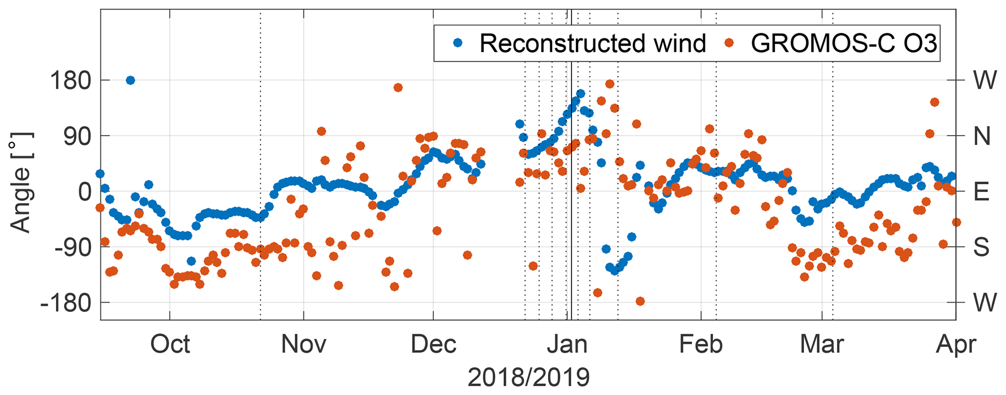
Figure 13 Direction of the horizontal wind field at Ny-Ålesund reconstructed from the stationary planetary waves 1 and 2 and the background wind, and the angle of the GROMOS-C ozone gradients at 3 hPa. The dotted lines indicate the dates of the polar vortex snapshots in Fig. 6 and the solid line shows the central date of the SSW.

5 Conclusions

We presented the co-located observations of middle-atmospheric ozone, water vapour and zonal and meridional wind profiles during the Arctic winter 2018/2019 and discussed the small-scale spatial variability of ozone at an altitude of 37 km (3 hPa). The ozone, water vapour and wind profiles were measured with two ground-based microwave radiometers which are located at the AWIPEV research base at Ny-Ålesund, Svalbard (79^∘ N, 12^∘ E). The ability to retrieve zonal and meridional wind profiles requires the measurement of ozone spectra in the four cardinal directions with a low observation angle. Besides the wind profiles, we retrieve from these spectra four separate ozone profiles along the lines of sight. At an altitude of 37 km the probed air masses in the E–W and N–S directions have a horizontal distance of 184 km. At Ny-Ålesund, which is located at 79^∘ N, this distance between the east and west measurement corresponds to 9.5^∘ longitude. With this unique measurement setup we are for the first time able to continuously monitor the ozone variability on a small spatial scale.

During winter 2018/2019 a major SSW took place. The central date, according to the MERRA-2 zonal wind reversal at 10 hPa, was 2 January. At Ny-Ålesund temperatures were increasing 50 K in the stratosphere at 10 hPa and decreasing by the same amount in the mesosphere at 0.1 hPa. The measured zonal and meridional wind speeds and ozone and water vapour VMRs are highly dependent on the location of the polar vortex during the SSW. At 10 hPa the ozone VMR almost doubled to 6.5 ppm when the polar vortex split. From SD-WACCM simulations we know that the net chemical ozone production is negative from October until mid March. Therefore we can attribute the ozone increase to enhanced meridional transport. The passing of the elongated Aleutian high-pressure system containing a low ozone pocket reduced ozone VMR at Ny-Ålesund by 25 % for a few days. At 0.3 hPa we found strong increases in water vapour VMR of 50 % which were followed by a steady decrease when the polar vortex reestablished and the air masses in the polar region were descending again. The wind field was highly variable because it strongly depends on the location of the polar vortex. The split of the polar vortex is visible in the wind measurements as enhanced meridional wind speeds.

From the ozone measurements in the four cardinal directions we calculated daily mean local ozone gradients for winter 2018/2019. At 20 km altitude (44 hPa) we found a relative magnitude of the ozone gradients of 4 % across a scale of 100 km and when Ny-Ålesund was inside of the polar vortex. This is in agreement with observations of Sparling et al. (2006). At higher altitudes (3 hPa) we found a seasonal variation in the magnitude and the orientation of the ozone gradients. Strong local gradients in the southward direction occurred in October and again in March, when the polar vortex was stable and the planetary wave activity low. From November on the amplitudes of the planetary waves 1 and 2 were growing until they broke down in the end of December and an SSW took place. The ozone gradients mainly point northward to eastward during this time period. The magnitudes decreased from October to November while the wave amplitudes were increasing. During the SSW the rapid mixing of air masses led to filamentary ozone structures and therefore to varying magnitude and angle of the ozone gradients. This was followed by a period of well-mixed ozone in the end of January when the polar vortex started to recover. Towards March the gradient magnitudes increased along with the zonal wind speed. The MERRA-2 reanalysis and the SD-WACCM model capture the seasonal variation in magnitude and angle of the ozone gradients. To link the changes in the ozone gradients with the planetary wave activity, we reconstructed the wind field at Ny-Ålesund from amplitude and phase of the planetary waves 1 and 2. We found a correlation of 0.4 between the angle of the ozone gradients and the direction of the reconstructed wind. Our results indicate that the ozone mixing above Ny-Ålesund during the winter season 2018/2019 was driven by the planetary wave activity of wave numbers 1 and 2, which disturbed the polar vortex and enabled a meridional transport inbound and outbound of the polar cap region, reducing the magnitude and changing the angle of the observed spatial ozone gradients from GROMOS-C. The presented measurements of GROMOS-C and MIAWARA-C point out that the VMR ratio of ozone and water vapour is not only driven by the chemistry in polar stratospheric clouds, but that it is also affected by dynamical processes due to planetary waves.