Global-scale distribution of ozone in the remote troposphere from the ATom and HIPPO airborne field missions

Ozone is a key constituent of the troposphere, where it drives photochemical processes, impacts air quality, and acts as a climate forcer. Large-scale in situ observations of ozone commensurate with the grid resolution of current Earth system models are necessary to validate model outputs and satellite retrievals. In this paper, we examine measurements from the Atmospheric Tomography (ATom; four deployments in 2016–2018) and the HIAPER Pole-to-Pole Observations (HIPPO; five deployments in 2009–2011) experiments, two global-scale airborne campaigns covering the Pacific and Atlantic basins.

ATom and HIPPO represent the first global-scale, vertically resolved measurements of O₃ distributions throughout the troposphere, with HIPPO sampling the atmosphere over the Pacific and ATom sampling both the Pacific and Atlantic. Given the relatively limited temporal resolution of these two campaigns, we first compare ATom and HIPPO ozone data to longer-term observational records to establish the representativeness of our dataset. We show that these two airborne campaigns captured on average 53 %, 54 %, and 38 % of the ozone variability in the marine boundary layer, free troposphere, and upper troposphere–lower stratosphere (UTLS), respectively, at nine well-established ozonesonde sites. Additionally, ATom captured the most frequent ozone concentrations measured by regular commercial aircraft flights in the northern Atlantic UTLS. We then use the repeated vertical profiles from these two campaigns to confirm and extend the existing knowledge of tropospheric ozone spatial and vertical distributions throughout the remote troposphere. We highlight a clear hemispheric gradient, with greater ozone in the Northern Hemisphere, consistent with greater precursor emissions and consistent with previous modeling and satellite studies. We also show that the ozone distribution below 8 km was similar in the extra-tropics of the Atlantic and Pacific basins, likely due to zonal circulation patterns. However, twice as much ozone was found in the tropical Atlantic as in the tropical Pacific, due to well-documented dynamical patterns transporting continental air masses over the Atlantic. Finally, we show that the seasonal variability of tropospheric ozone over the Pacific and the Atlantic basins is driven year-round by transported continental plumes and photochemistry, and the vertical distribution is driven by photochemistry and mixing with stratospheric air. This new dataset provides additional constraints for global climate and chemistry models to improve our understanding of both ozone production and loss processes in remote regions, as well as the influence of anthropogenic emissions on baseline ozone.

1 Introduction

Tropospheric ozone (O₃) plays a major role in local, regional, and global air quality and significantly influences Earth's radiative budget (IPCC, 2013; Shindell et al., 2012). In addition, O₃ drives tropospheric photochemical processes by controlling hydroxyl radical (OH) abundance, which subsequently controls the lifetime of other pollutants including volatile organic compounds (VOCs), methane, and some stratospheric ozone-depleting substances (Crutzen, 1974; Levy, 1971). Sources of O₃ to the troposphere include downward transport from the stratosphere (Junge, 1962) and photochemical production from precursors such as carbon monoxide (CO), methane (CH₄), and VOCs in the presence of nitrogen oxides (NO_x) from natural or anthropogenic sources (Monks et al., 2009). Tropospheric O₃ sinks include photodissociation, chemical reactions, and dry deposition. Owing to its relatively long lifetime (∼23 d in the troposphere; Young et al., 2013), O₃ can be transported across hemispheric scales. Thus, O₃ mixing ratios over a region depend not only on local and regional sources and sinks but also on long-range transport. Further, the uneven density of O₃ monitoring locations around the globe leads to significant sampling gaps, especially near developing nations and away from land (Gaudel et al., 2018). The troposphere over the remote oceans is among the least-sampled regions, despite hosting 60 %–70 % of the global tropospheric O₃ burden (Holmes et al., 2013).

Since the early 1980s, several aircraft campaigns have addressed this paucity of remote observations, most notably under the umbrella of the Global Tropospheric Experiment (GTE), a major component of the National Aeronautics and Space Administration (NASA) Tropospheric Chemistry Program (https://www-gte.larc.nasa.gov, last access: 9 April 2020). Airborne campaigns have targeted both the Pacific and Atlantic oceans, providing novel characterization of O₃ sources, distribution, and photochemistry in the marine troposphere (Browell et al., 1996a; Davis et al., 1996; Jacob et al., 1996; Pan et al., 2015; Schultz et al., 1999; Singh et al., 1996c) and the low-O₃ tropical Pacific pool (Singh et al., 1996b); the pervasive role of continental outflow on O₃ production (Bey et al., 2001; Crawford et al., 1997; Heald et al., 2003; Kondo et al., 2004; Martin et al., 2002; Zhang et al., 2008); and the marked influence of African and South American biomass burning on O₃ production in the Southern Hemisphere (Browell et al., 1996b; Fenn et al., 1999; Mauzerall et al., 1998; Singh et al., 1996a; Thompson et al., 1996). Ozonesondes have been launched from remote sites for more than 3 decades in some places and have provided additional constraints on the sources and photochemical balance of tropospheric O₃, including a deep understanding of the vertically resolved tropospheric O₃ climatology in select locations (Derwent et al., 2016; Diab et al., 2004; Jensen et al., 2012; Kley et al., 1996; Liu et al., 2013; Logan, 1985; Logan and Kirchhoff, 1986; Newton et al., 2018; Oltmans et al., 2001; Parrish et al., 2016; Sauvage et al., 2006; Thompson et al., 2012). Spatially resolved O₃ climatology has been provided from routine sampling by commercial aircraft, which has mostly been limited to the upper troposphere or over continental regions (Clark et al., 2015; Cohen et al., 2018; Logan et al., 2012; Petetin et al., 2016; Sauvage et al., 2006; Thouret et al., 1998; Zbinden et al., 2013), and by satellite observations (Edwards et al., 2003; Fishman et al., 1990, 1991; Hu et al., 2017; Thompson et al., 2017; Wespes et al., 2017; Ziemke et al., 2005, 2006, 2017), which have been somewhat tempered by large uncertainties (Tarasick et al., 2019b). Recent overview analyses depict the current understanding of global tropospheric O₃ sources, distribution, and photochemical balance and underscore the insufficiency of observations in the remote free troposphere (Cooper et al., 2014; Gaudel et al., 2018; Tarasick et al., 2019b) necessary to improve the current representation of tropospheric O₃ in global chemical models (Young et al., 2018). The spatial and temporal representativeness of O₃ observations is currently the biggest source of uncertainty when inferring O₃ climatology in the free troposphere, even in regions where observation are abundant but not ideally distributed (Lin et al., 2015b; Tarasick et al., 2019b). Most studies reporting the global O₃ distribution use satellite observations (Edwards et al., 2003; Fishman et al., 1990, 1991; Thompson et al., 2017; Wespes et al., 2017; Ziemke et al., 2005, 2006, 2017), modeling analyses (Hu et al., 2017), or observations spatially expanded using back trajectory calculations (e.g., Liu et al., 2013; Tarasick et al., 2010). While useful, these studies come with somewhat large uncertainties, as recently noted by reports from the Tropospheric Ozone Assessment Report (TOAR), and thus require additional in situ observations to be used as a validation benchmark (Tarasick et al., 2019b; Young et al., 2018).

The Atmospheric Tomography (ATom, https://espo.nasa.gov/atom, last access: 9 April 2020) mission was a NASA Earth Venture airborne field project to address the sparseness of atmospheric observations over remote ocean regions by systematically sampling the troposphere over the Pacific and Atlantic basins along a global-scale circuit (Fig. 1). ATom deployed an extensive payload on the NASA DC-8 aircraft, measuring a wide range of chemical, microphysical, and meteorological parameters in repeated vertical profiles from 0.2 km to over 13 km in altitude, from the Arctic to the Antarctic over the Pacific and Atlantic oceans, in four separate seasons from 2016 to 2018. ATom built on a previous study, the HIAPER Pole-to-Pole Observations (HIPPO, https://www.eol.ucar.edu/field_projects/hippo, last access: 9 April 2020) mission. The goal of HIPPO was to measure atmospheric distributions of important greenhouse gases and reactive species over the Pacific Ocean, from the surface to the tropopause, five times during different seasons from 2009 to 2011. Together, ATom and HIPPO provide recent and comprehensive information about the altitudinal, latitudinal, and seasonal composition of the remote troposphere over the Pacific, and ATom also provides this information over the Atlantic. In addition, ATom and HIPPO sampling strategies were designed to deliver an objective climatology of key species to enable the modeling of the air parcel reactivity of the remote troposphere (Prather et al., 2017).

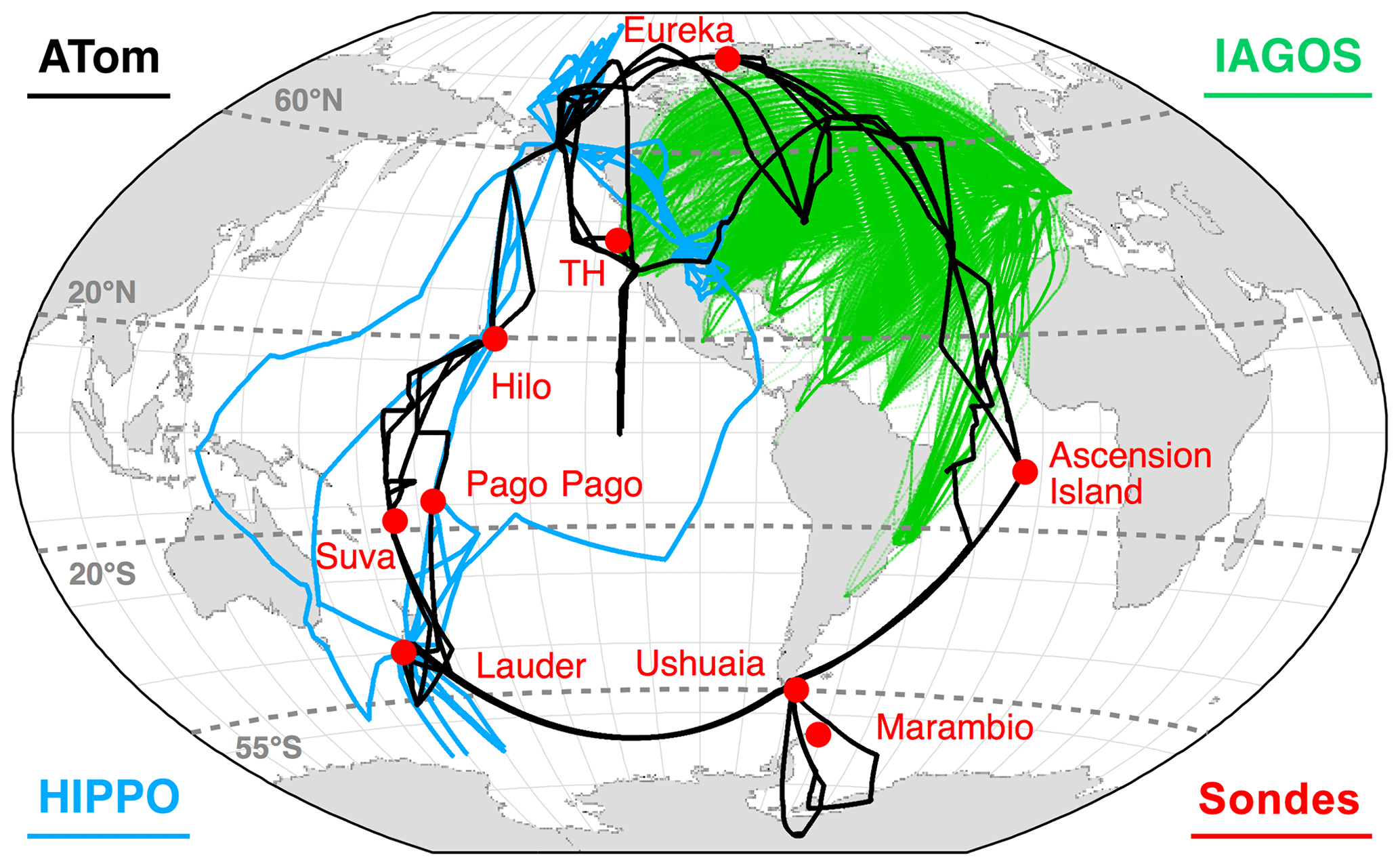
Figure 1 The location and flight tracks of all O₃ monitoring platforms used in this work are illustrated using different markers and colors. The ATom flight track is in black, the HIPPO flight track is in blue, IAGOS flight paths are in green, and the ozonesonde launching sites are indicated by the red markers. The dotted gray lines define the latitudinal bands over which individual ATom and HIPPO profiles were averaged to derive a regional O₃ distribution: the tropics (20^∘ S–20^∘ N), the midlatitudes (55–20^∘ S, 20–60^∘ N), and the high latitudes (90–55^∘ S, 60–90^∘ N). Only data from remote oceanic flight segments of ATom and HIPPO missions were used in this work.

Here we use existing ozonesonde and commercial aircraft observations of O₃ at selected locations along the ATom and HIPPO circuits to provide a climatological context for the altitudinal, latitudinal, and seasonal distributions of O₃ derived from the systematic airborne in situ “snapshots”. Long-term O₃ observations are obtained from decades of ozonesonde vertical profiles (e.g., Oltmans et al., 2013; Thompson et al., 2017) and from ∼60 000 flights using the In-service Aircraft for a Global Observing System (IAGOS) infrastructure (Petzold et al., 2015; http://www.iagos.org, last access: 9 April 2020). Ozonesondes have typically been launched weekly for 2 decades or more, depending on the site, and have sampled a wide range of air masses across the globe, from O₃-poor remote surface locations to the O₃-rich stratosphere. IAGOS commercial aircraft have provided daily measurements in the upper troposphere and lower stratosphere (UTLS) for the past 25 years, especially over the northern midlatitudes between America and Europe. Combined, the ozonesonde and IAGOS datasets offer robust measurement-based climatologies that quantify the full expected range of atmospheric O₃ variability with altitude and season.

The in situ data from temporally limited intensive field studies can be placed in context by comparing them with long-term ozonesonde and commercial aircraft monitoring data. Evaluating the representativeness of in situ observations from airborne campaigns by comparing them to longer-term observational records is a critical exercise never before done at such a global scale. We show that ATom and HIPPO measurements capture the spatial and, in some cases, temporal dependence of O₃ in the remote atmosphere, thereby highlighting the usefulness of airborne observations to fill in the gaps of established but limited O₃ climatologies and other similarly long-lived species. Then, we use the geographically extensive ATom and HIPPO vertical profile data to establish a more complete measurement-based benchmark for O₃ abundance and distribution in the remote marine atmosphere.

2 Measurements

2.1 ATom

The four ATom circuits occurred in July–August 2016 (ATom-1), January–February 2017 (ATom-2), September–October 2017 (ATom-3), and April–May 2018 (ATom-4); thus, they spanned all four seasons in both hemispheres over a 2-year timeframe (Table S1 in the Supplement). In total, the mission consisted of 48 science flights and 548 vertical profiles distributed nearly equally along the global circuit. All four deployments completed roughly the same loop, starting and ending in Palmdale, California, USA (Fig. 1). A notable addition during ATom-3 and ATom-4 were out-and-back flights from Punta Arenas, Chile, to sample the Antarctic troposphere and UTLS.

O₃ was measured using the National Oceanic and Atmospheric Administration (NOAA) nitrogen oxides and ozone (NO_yO₃) instrument. The O₃ channel of the NO_yO₃ instrument is based on the gas-phase chemiluminescence (CL) detection of ambient O₃ with pure NO added as a reagent gas (Ridley et al., 1992; Stedman et al., 1972). Ambient air is continuously sampled from a pressure-building ducted aircraft inlet into the NO_yO₃ instrument at a typical flow rate of 1025.0±0.2 standard cubic centimeters per minute (sccm) in flight. Pure NO reagent gas flow delivered at 3.450±0.006 sccm is mixed with sampled air in a pressure (8.00±0.08 Torr) and temperature (24.96±0.01 ^∘C) controlled reaction vessel. NO-induced CL is detected with a dry-ice-cooled, red-sensitive photomultiplier tube and the amplified digitized signal is recorded using an 80 MHz counter; pulse coincidence corrections at high count rates were applied, but they are negligible for the data presented in this work. The instrument sensitivity for measuring O₃ under these conditions is 3150±80 counts per second per part per billion by volume (ppbv) averaged over the entire ATom circuit. CL detector calibrations were routinely performed both on the ground and during flight by standard addition of O₃ produced by irradiating ultrapure air with 185 nm UV light and were independently measured using UV optical absorption at 254 nm. All O₃ measurements were taken at a temporal resolution of 10 Hz, averaged to 1 Hz, and corrected for the dependence of instrument sensitivity on ambient water vapor content (Ridley et al., 1992). Under these conditions the total estimated 1 Hz uncertainty at sea level is ± (0.015 ppbv +2 %).

A commercial dual-beam photometer (2B Technologies Model 211) based on UV optical absorption at 254 nm also measured O₃ on ATom, with an estimated uncertainty of ± (1.5 ppbv +1 %) at a 2 s sampling resolution. Comparison of the 2B absorption instrument O₃ data to the NO_yO₃ CL instrument O₃ data agreed to within combined instrumental uncertainties, lending additional confidence to the NO_yO₃ CL instrument calibration. For the ATom project, we use NO_yO₃ instrument O₃ data in the following analyses.

Data from two CO measurements were combined in this analysis. The Harvard quantum cascade laser spectrometer (QCLS) instrument used a pulsed quantum cascade laser tuned at ∼2160 cm⁻¹ to measure the absorption of CO through an astigmatic multi-pass sample cell with 76 m path length and detection using a liquid-nitrogen-cooled HgCdTe detector (Santoni et al., 2014). In-flight calibrations were conducted with gases traceable to the NOAA World Meteorological Organization (WMO) X2014A scale, and the QCLS observations have an accuracy and precision of 3.5 and 0.15 ppb for 1 Hz data, respectively. CO was also measured by the NOAA cavity ring-down spectrometer (CRDS, Picarro, Inc., model G2401-m; Karion et al., 2013) in the 1.57 µm region with a total uncertainty of 5.0 ppbv for 1 Hz data. The NOAA Picarro data were also reported on the World Meteorological Organization (WMO) X2014A scale. The combined CO data (CO-X) used here correspond to the QCLS data, with the Picarro measurement used to fill calibration gaps in the QCLS time series.

Water (H₂O) vapor was measured using the NASA Langley Diode Laser Hygrometer (DLH), an open-path infrared absorption spectrometer that uses a laser locked to a water vapor absorption feature at ∼1.395 µm. Raw data are processed at the instrument's native ∼100 Hz acquisition rate and averaged to 1 Hz with an overall measurement accuracy within 5 %.

2.2 HIPPO

The HIPPO mission consisted of five seasonal deployments over the Pacific Basin between 2009 and 2011, from the North Pole to the coastal waters of Antarctica (Wofsy, 2011). HIPPO deployments consisted of two transects, southbound and northbound, and occurred in January 2009 (HIPPO-1), October–November 2009 (HIPPO-2), March–April 2010 (HIPPO-3), June–July 2011 (HIPPO-4), and August–September 2011 (HIPPO-5). The platform used was the NSF Gulfstream V (GV) aircraft. More details can be found in Table S1.

A NOAA custom-built dual-beam photometer based on UV optical absorption at 254 nm was used to measure O₃ (Proffitt and McLaughlin, 1983). The uncertainty of the 1 Hz O₃ data is estimated to be ± (1 ppbv +5 %) for 1 Hz data. A commercial dual-beam O₃ photometer (2B Technologies Model 205) based on UV optical absorption at 254 nm was also included in the HIPPO payload. Comparison of the 2B O₃ data to the NOAA O₃ data showed general agreement within combined instrument uncertainties on level flight legs. For the HIPPO project, we use NOAA O₃ data in the following analyses.

Data from two CO measurements were combined in this analysis. The QCLS instrument was the same instrument as that used during ATom and is described in Sect. 2.1. CO was also measured by an Aero-Laser AL5002 instrument using vacuum UV resonance fluorescence (in the 170–200 nm range) with an uncertainty of ± (2 ppbv +3 %) at a 2 s sampling resolution. The combined CO data (CO-X) used here correspond to the QCLS data, with the Aero-Laser measurement used to fill calibration gaps in the QCLS time series.

2.3 IAGOS

IAGOS is a European Research Infrastructure that provides airborne in situ chemical, aerosol, and meteorological measurements using commercial aircraft (Petzold et al., 2015). The IAGOS Research Infrastructure includes data from both the CARIBIC (Civil Aircraft for the Regular Investigation of the atmosphere Based on an Instrument Container; Brenninkmeijer et al., 2007) and MOZAIC (Measurements of OZone and water vapor by Airbus In-service airCraft; Marenco et al., 1998) programs, providing measurements from ∼60 000 flights since 1994. We note the relative lack of IAGOS data over the Pacific compared with the Atlantic (shorter temporal record, lower flight frequency, and fewer flights with concomitant O₃ and CO measurements) and, therefore, limited the comparison to the Atlantic. Because commercial aircraft cruise altitudes over the ocean are predominantly between 9 and 12 km, the comparison between ATom and IAGOS is further limited to the UTLS (Fig. 1). More details are shown in Table S1.

Identical dual-beam UV absorption photometers measured O₃ aboard the IAGOS flights. An instrument comparison demonstrated that the photometers (standard Model 49, Thermo Scientific, modified for aircraft use) showed good consistency in measuring O₃ (Nédélec et al., 2015). The associated uncertainty is ± (2 ppbv +2 %) at a 4 s sampling resolution (Thouret et al., 1998).

CO measurements were made using infrared absorption photometers (standard Model 48 Trace Level, Thermo Scientific, modified for aircraft use) with an uncertainty of ± (5 ppbv +5 %) at a 30 s sampling resolution (Nédélec et al., 2003, 2015).

2.4 Ozonesondes

Ozonesondes have measured the vertical distribution of O₃ in the atmosphere for decades, and they provide some of the longest tropospheric records that are commonly used to determine regional O₃ trends (Gaudel et al., 2018; Leonard et al., 2017; Oltmans et al., 2001; Tarasick et al., 2019a; Thompson et al., 2017). Ozonesonde launching sites are operated by the NOAA Earth System Research Laboratory (ESRL) Global Monitoring Laboratory (GML), NASA Goddard's Southern Hemisphere Additional OZonesondes (SHADOZ) program, the New Zealand National Institute of Water & Atmospheric Research (NIWA), the National Meteorological Center of Argentina in collaboration with the Finnish Meteorological Institute (FMI), or Environment and Climate Change Canada. A more detailed description of each ozonesonde site and the corresponding dataset can be found in Tables S1 and S2. All sites use electrochemical concentration cell (ECC) ozonesondes that rely on the potassium iodide electrochemical detection of O₃ and that provide a vertical resolution of about 100 m (Komhyr, 1969). The associated uncertainty is usually ± (5 %–10 %) (Tarasick et al., 2019b; Thompson et al., 2019; Witte et al., 2018).

2.5 Data analysis

In this analysis, ATom flight tracks were divided into the Atlantic and Pacific basins and then further subdivided into five regions within those basins: the tropics and the northern and southern middle and high latitudes. Vertical profiles presented graphically in this paper show O₃ median values and the 25th to 75th percentile range within the 0–12 km tropospheric column sampled by the DC-8 aircraft. These medians were obtained by averaging with equal weight the individual profiles within each region over 1 km altitude bins.

HIPPO flight tracks are illustrated in Fig. 1. The flight segments used for comparison with ATom were binned into the same Pacific latitude and longitude bands as for ATom. HIPPO vertical profile data are derived using the same methodology as for ATom.

All IAGOS flight tracks over the northern and tropical Atlantic are represented in Fig. 1 in green. The latitude bands used to parse IAGOS data are consistent with those used for ATom. The longitude bands are 50–20^∘ W in the tropics, 50–10^∘ W in the northern midlatitudes, and 110–10^∘ W in the northern high latitudes. Variation of the longitude band widths does not significantly affect the O₃ distributions measured by IAGOS. Data from all flights from 1994 to 2017 were included in the IAGOS dataset considered here, and they were then divided into two altitude bins (8–10 and 10–12 km) in order to better understand the influence of different O₃ sources (e.g., anthropogenic, stratospheric) on these two layers of the atmosphere.

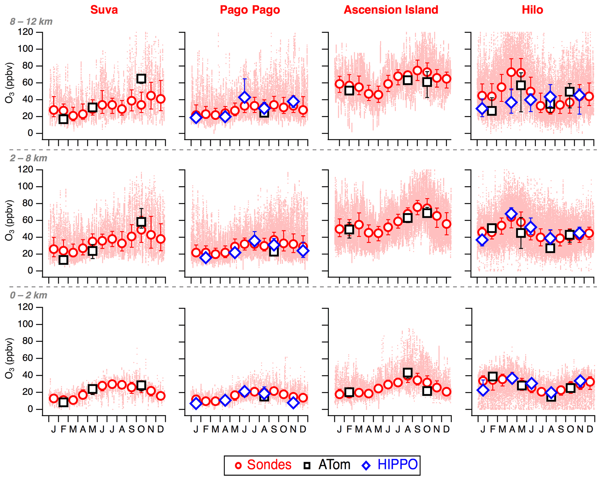
Figure 2 Comparison of ATom (black squares) and HIPPO (blue diamonds) monthly median O₃ with ozonesonde (red circles) records from the four tropical sites. Markers indicate the median, and the bars indicate the 25th and 75th percentiles. The three rows, from bottom to top, correspond to the boundary layer (0–2 km), the free troposphere (2–8 km), and the UTLS (8–12 km). The pink dots show every O₃ data point measured by ozonesondes for the timeframes indicated in Table S2.

We compare the ozonesonde measurements to ATom and HIPPO aircraft data sampled within 500 km of each ozonesonde launching site, as we expect a robust correlation in the free troposphere within this distance (Liu et al., 2009). We used the surface coordinates of the ozonesonde sites because the in-flight coordinates of ozonesondes are not available for all sites. For comparison with ozonesonde long-term records, we consider three regions of the atmosphere: the boundary layer (0–2 km), the free troposphere (2–8 km), and the UTLS (8–12 km). For each layer, we compared monthly O₃ distributions from ozonesondes with the corresponding seasonal O₃ distributions from aircraft measurements using the skill score (S_score) metric (Perkins et al., 2007). The S_score is calculated by summing the minimum probability of two normalized distributions at each bin center; therefore, it measures the overlapping area between two probability distribution functions. If the distributions are identical, the skill score will equal 100 % (see Fig. S1 for further examples). Note that the S_score is positively correlated with the size of the bin used to compare distributions. Here we chose a bin size of 5 ppbv, which is larger than the combined precision of ATom, HIPPO, and IAGOS measurements but is small enough to separate distinct air masses and their influence on the O₃ distribution. Variables such as the distance to each ozonesonde launching site (500 km in this study), the bin size of the O₃ distributions (5 ppbv in this study), and the length of each ozonesonde record (full length in this study) can shift the vertically averaged S_score value by up to 8 % (Table S3). Therefore, we treat this 8 % as a rough estimate of the precision of the S_score values presented here.

All three techniques (chemiluminescence, UV absorption, and ECC) used to measure O₃ for the datasets analyzed in this work have been shown to provide directly comparable accurate measurements with well-defined uncertainties (Tarasick et al., 2019b).

2.6 Back trajectory analysis

Analysis of back trajectories for air masses sampled during airborne missions is useful to examine the air mass source regions and causes of O₃ variability over the Pacific and Atlantic oceans. We calculated 10 d back trajectories using the TRAJ3D model (Bowman, 1993; Bowman and Carrie, 2002) and National Centers for Environmental Prediction (NCEP) global forecast system (GFS) meteorology. Trajectories were initialized each minute along all of the ATom flight tracks.

3 Comparison of ATom and HIPPO O₃ distributions to longer-term observational records

Here we use existing ozonesonde and IAGOS observations of O₃ at selected locations along the ATom and HIPPO circuits to provide a climatological context for O₃ distributions derived from the systematic airborne in situ “snapshots”. We quantify how much of O₃ variability, occurring on timescales ranging from hours to decades, was captured by the temporally limited HIPPO and ATom missions.

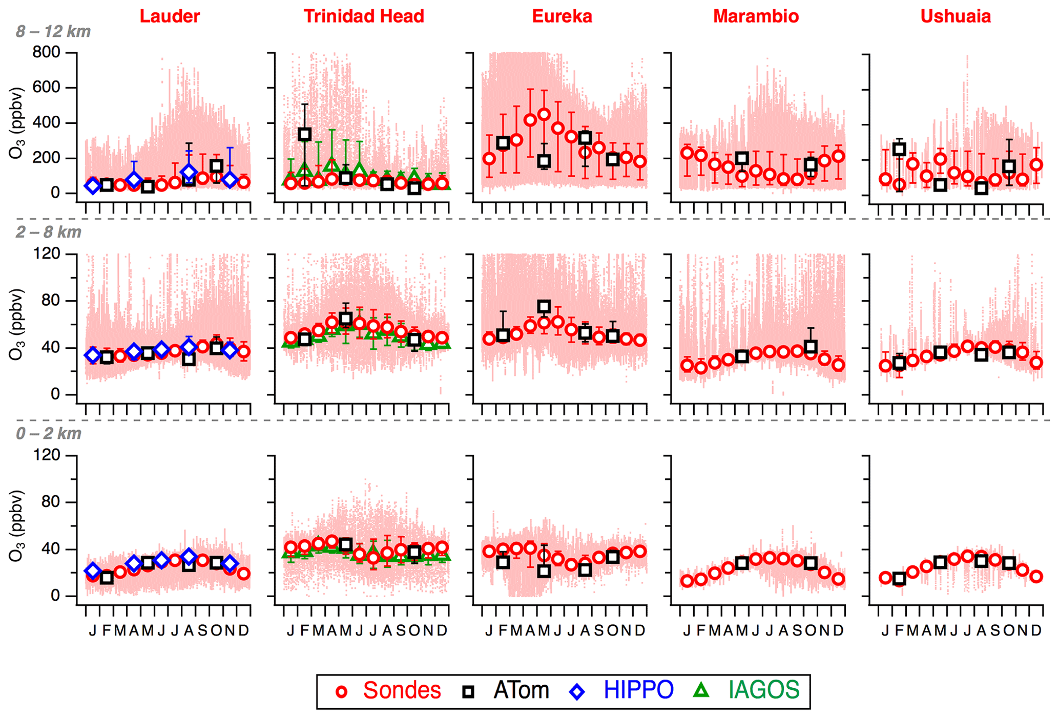
Figure 3 Same as in Fig. 2 but for ozonesonde launching sites located in the middle and high latitudes. O₃ data obtained from the IAGOS program (green triangles) during descents into San Francisco Bay Area airports were also added to the Trinidad Head site for comparison.

3.1 Comparison to ozonesondes

ATom and HIPPO explored the fidelity with which airborne missions represent O₃ climatology in the remote troposphere. Here, we show that aircraft-measured median O₃ follows the seasonal ozonesonde-measured median O₃ cycle at most of the sites studied in this paper, as well as at almost all altitudes – with a few exceptions (Figs. 2, 3). Figure 2 plots the monthly median O₃ measurements from the tropical ozonesonde sites in three altitude bins, along with the median values obtained from HIPPO and ATom measurements. Figure 3 plots the same for the extra-tropical sites. Figure 4 correlates the median O₃ measured by aircraft in Figs. 2 and 3 with those measured by ozonesondes. At the Eureka site, the winter and spring ATom deployments recorded a significantly lower median O₃ compared with the corresponding ozonesonde monthly median O₃ in the 0–2 km range (Fig. 3). Eureka is frequently subject to springtime O₃ depletion events at the surface due to atmospheric bromine chemistry, which is well documented by the ozonesonde record (Fig. 3; Tarasick and Bottenheim, 2002). Sampling during O₃ depletion events significantly lowered the ATom winter and springtime O₃ distributions near this site. In the 2–8 km range, there is a very good seasonal agreement between ATom/HIPPO and the ozonesondes (Fig. 4b). Most seasonal differences are found above 8 km (e.g., ATom in February at Trinidad Head and in May at Eureka; Fig. 3) and can be linked to the occurrence – or absence – of stratospheric air sampling during ATom and HIPPO. In the absence of stratospheric air mixing (<8 km in Fig. 4), ATom/HIPPO successfully capture a large fraction of O₃ climatology everywhere (Fig. 4b, c).

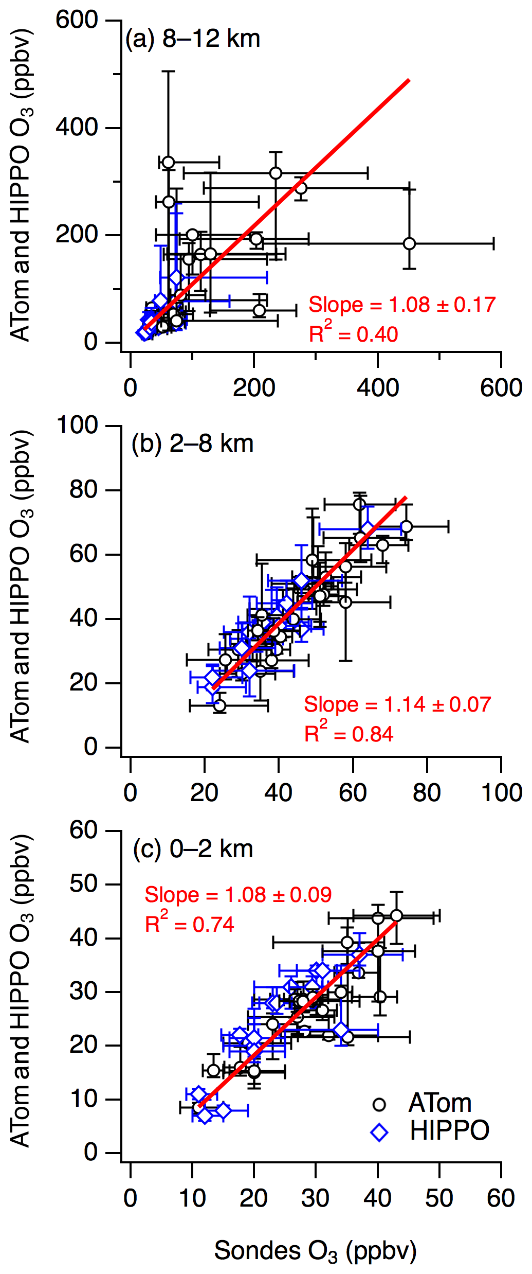
Figure 4 ATom (black circles) and HIPPO (blue diamonds) combined monthly median O₃ vs. monthly median O₃ from ozonesondes at the nine sites considered in this study. The three panels indicate the correlations for (a) the UTLS (8–12 km), (b) the free troposphere (2–8 km), and (c) the boundary layer (0–2 km). The orthogonal regression fits are two-sided but not weighted.

Figures 5 and 6 show vertical profiles of O₃ distributions by season at each ozonesonde site, along with comparisons to HIPPO and ATom vertical profiles. Our analysis reveals that O₃ distributions derived from the ATom and HIPPO seasonal “snapshots” capture 30 %–71 % of the 1 km vertically binned O₃ distribution established by long-term ozonesonde climatologies. For the nine ozonesonde sites considered here, ATom and HIPPO captured on average 53 %, 54 %, and 38 % of the O₃ distribution in the 0–2, 2–8, and 8–12 km altitude bins, respectively.

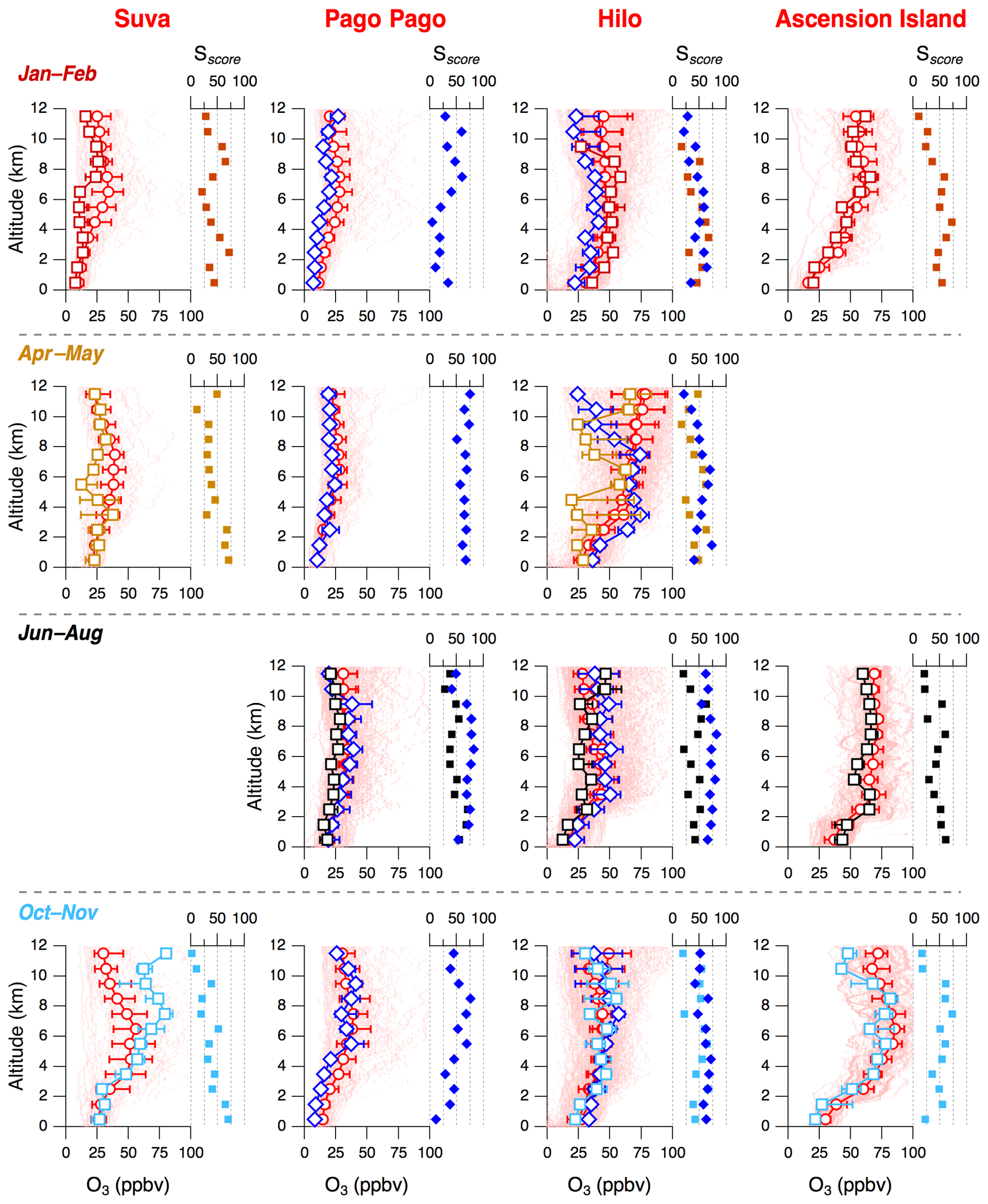
Figure 5 Seasonal comparison of 1 km vertically binned ATom (colored squares) and HIPPO (blue diamonds) median O₃ with ozonesonde (red circles) records at four sites in the tropics (Suva in Fiji, Pago Pago in American Samoa, Hilo in Hawaii, and Ascension Island). Markers indicate the median, and the bars are the 25th and 75th percentiles. The S_score is a metric of how well ATom and HIPPO 1 km binned O₃ probability distribution functions (PDFs) overlap with the corresponding 1 km binned O₃ PDFs from ozonesondes. The S_score shown using squares compares ATom with ozonesondes, and the S_score shown using blue diamonds compares HIPPO with ozonesondes. The pink dots show every O₃ data point measured by ozonesondes for the timeframes indicated in Table S2.

Figure 6 Same as in Fig. 5 but for ozonesonde launching sites located in middle and high latitudes (Lauder in New Zealand, Trinidad Head in the USA, Eureka in Canada, Ushuaia in Argentina, and Marambio in Antarctica). O₃ data obtained from the IAGOS program (green triangles) during descents into San Francisco Bay Area airports were also added to the Trinidad Head site for comparison.

Larger differences between ATom/HIPPO and the ozonesonde records in the UTLS (8–12 km) can be ascribed to O₃ variability from stratospheric–tropospheric exchange, which is not always captured by the ATom and HIPPO missions. This increased O₃ variability in the UTLS is well described by the long-term ozonesonde records at Lauder, Trinidad Head, Eureka, Ushuaia, and Marambio (Figs. 3, 6). In these middle- and high-latitude locations in both hemispheres, O₃ variability is especially pronounced during winter and spring, time periods favorable to more frequent stratospheric air mixing (Greenslade et al., 2017; Lin et al., 2015a; Tarasick et al., 2019a). Furthermore, the probability of sampling stratospheric air masses at the ATom and HIPPO ceiling altitude (12–14 km) increases with latitude, resulting in a lower S_score between the ATom/HIPPO and ozonesonde datasets at the extra-tropical sites than at the tropical sites (Fig. S2a and b in the Supplement).

In the boundary layer (0–2 km) of the remote troposphere, O₃ variability is predominantly impacted by loss mechanisms. Ozonesonde records show instances of O₃ mixing ratios lower than 10 ppbv throughout the year in the boundary layer at the nine sites studied here (Figs. 2, 3). The lowest O₃ mixing ratios are a result of (a) photochemical destruction over the oceans in the tropics (Monks et al., 1998, 2000; Thompson et al., 1993), (b) O₃-destroying halogen emissions in polar regions in springtime (e.g., Fan and Jacob, 1992), and (c) transport of O₃-poor oceanic air over the midlatitude sites (e.g., Neuman et al., 2012).

ATom and HIPPO best describe the O₃ distribution in the free troposphere (2–8 km; Figs. S2a, b). This suggests that airborne campaigns can capture global baseline O₃ values, along with the long-range transport of O₃ pollution plumes that are often lofted to this altitude range and are responsible for O₃ variability.

While ATom consisted of one transect per ocean per season, HIPPO covered the Pacific twice per seasonal deployment (southbound and northbound). The 1 km binned S_score was on average higher when two combined seasonal HIPPO transects (southbound and northbound) were available to compare to ozonesonde records, as opposed to when comparing O₃ profiles from individual HIPPO transects (Fig. S2c). In addition, two seasonal transects during HIPPO reduced the occurrence of low S_score values. The S_score decrease from flying only one Pacific transect during ATom was traded for the increase of vertical profiles over the Atlantic Basin, which was not sampled during HIPPO. Future airborne missions with multiple seasonal vertical profiles over large-scale regions would be ideal to better depict the full range of tropospheric O₃ variability.

3.2 Comparison to IAGOS

IAGOS O₃ and CO observations in the northern Atlantic UTLS provide a measurement-based climatology at commercial aircraft cruise altitudes for comparison to ATom. Simultaneous measurements of O₃ and CO are of particular interest because CO provides a long-lived tracer of continental emissions, which helps to differentiate O₃ sources (Cohen et al., 2018). We note that while IAGOS measurements encompass hundreds of seasonal flights (depending on the region), ATom sampled within each latitude band and season on one or two flights only (Fig. 1). Thus, variability in the UT that occurred on timescales longer than a day was not captured by ATom. Consequently, it is not surprising to see that ATom systematically under-sampled tropospheric O₃ (and CO) variability compared with IAGOS at all latitudes in the northern Atlantic (Figs. 7, 8). ATom captured on average 40 % of the O₃ variability measured by IAGOS in the Atlantic UTLS (Fig. 7), which is on par with the S_score of 38 % obtained when comparing ATom and HIPPO to ozonesonde data (see Sect. 3.1).

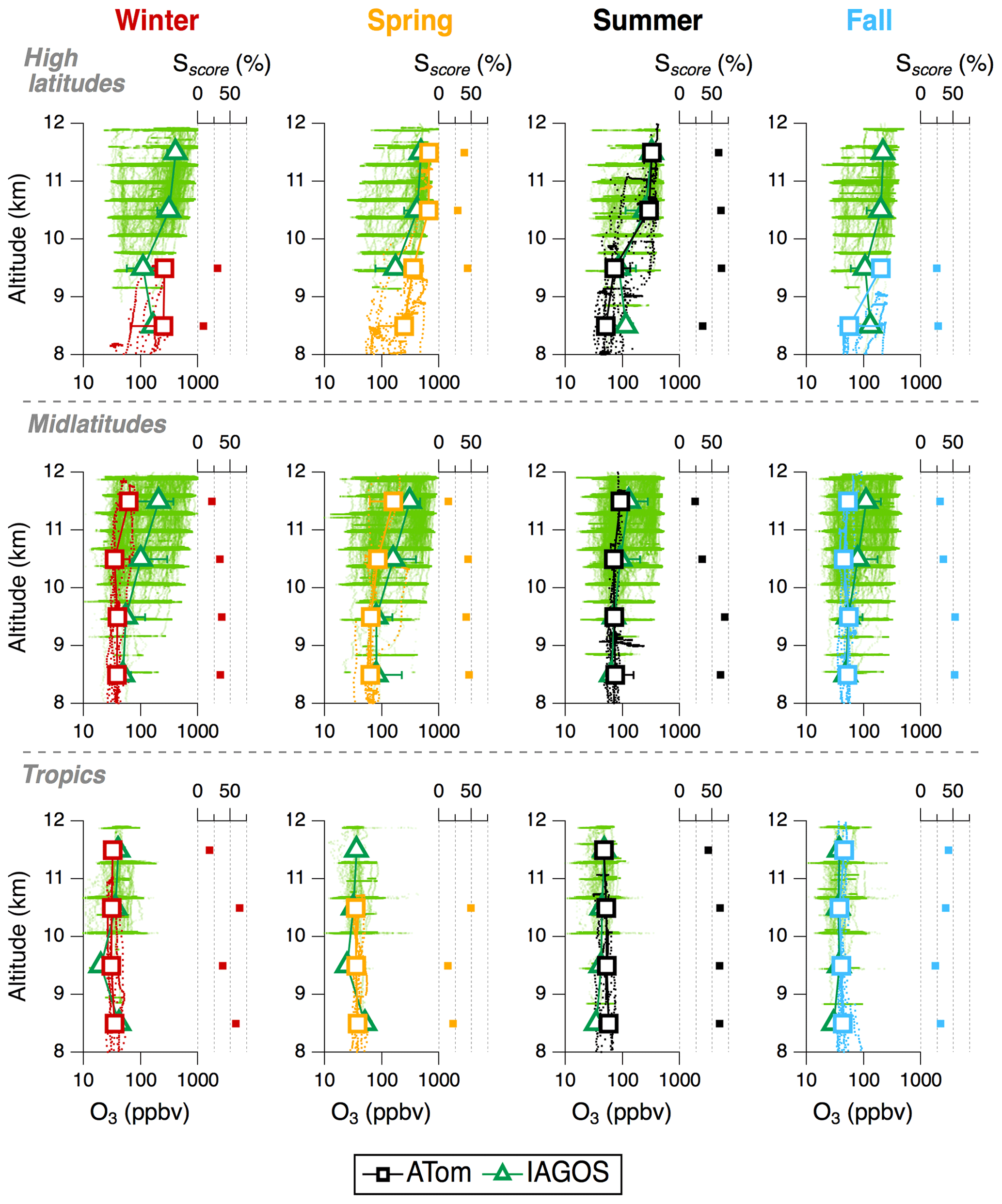
Figure 7 Seasonal comparison of 1 km binned ATom (colored squares) median O₃ with IAGOS (green triangles) in the northern Atlantic UTLS. Markers indicate the median, and the bars are the 25th and 75th percentiles. The three different rows indicate the latitudinal bands. The four columns indicate the seasons. The green dots show every O₃ data point measured by IAGOS flights for the timeframe indicated in Table S1.

In the middle and high latitudes, the shapes of the O₃ vs. CO scatterplots from IAGOS data demonstrate that distinct sources contribute to O₃ levels in the UTLS (Fig. 8a, b; Gaudel et al., 2015). The high O₃ (>150 ppbv)–low CO (<100 ppbv) range corresponds to intrusions of stratospheric air, which were mostly sampled in the spring season during ATom, supporting previous observations of increased stratospheric air mixing during this season (Lin et al., 2015a; Tarasick et al., 2019a). The low O₃ (<50 ppbv)–low CO (<100 ppbv) range corresponds to the tropospheric baseline air, whereas the intermediate O₃ (50–120 ppbv)–high CO (>100 ppbv) range generally represents the influence of air masses transported from continental regions. During ATom, high O₃ and low CO in the middle- and high-latitude UTLS were typical of stratospheric and baseline tropospheric air mixing.

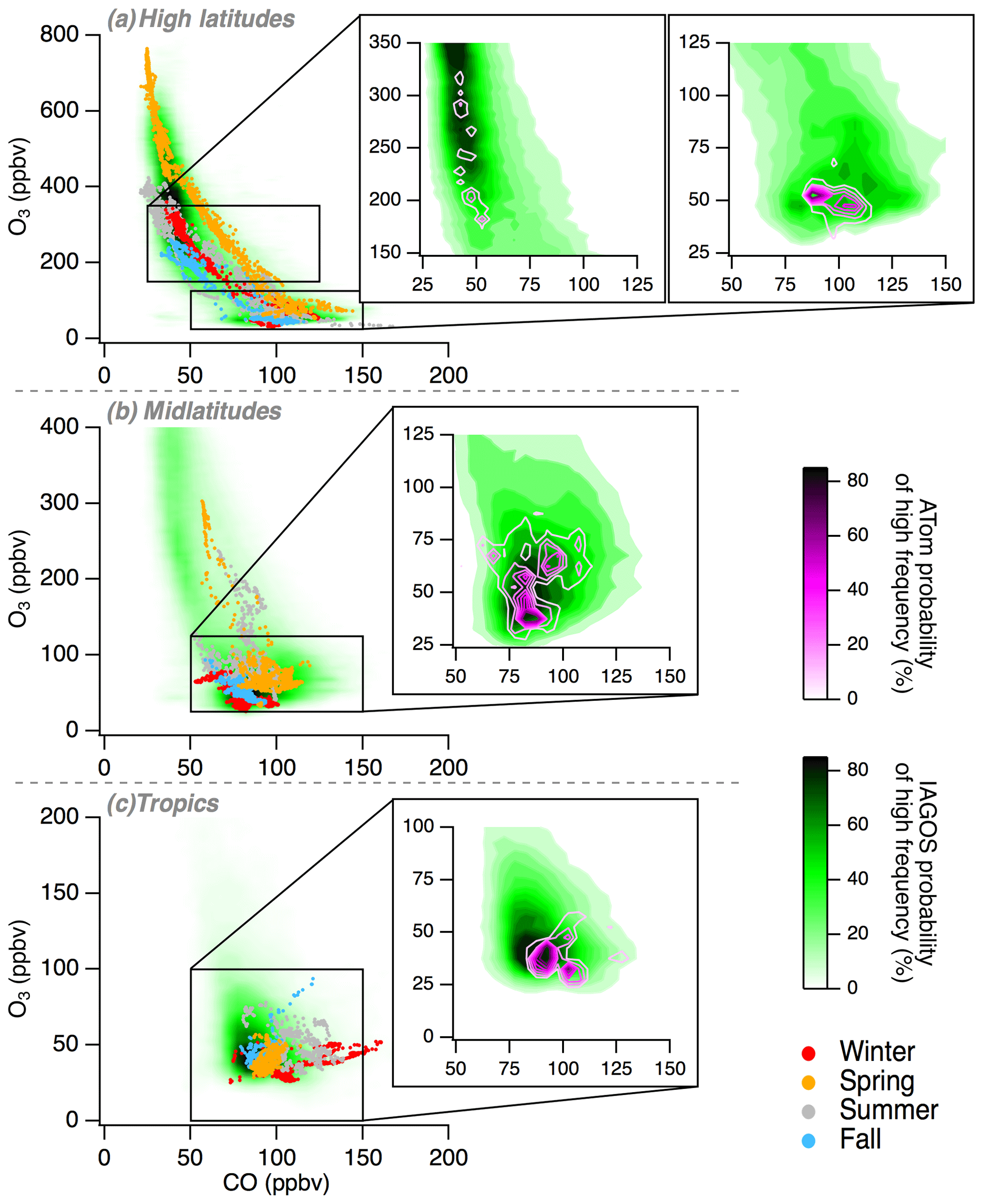
Figure 8 IAGOS and ATom seasonal O₃ vs. CO scatterplots, with insets showing the most frequent O₃ values measured during IAGOS and ATom. ATom seasonal deployments are colored according to the legend. The frequency gradient of the O₃ counts is illustrated by the color scales (green for IAGOS and magenta for ATom). ATom measurements have been combined for the frequency gradients shown in the insets. The probability of high frequency refers to the probability of finding frequently measured O₃ values within the contour boundaries.

O₃ measured during IAGOS rarely exceeds 150 ppbv in the northern tropical Atlantic UTLS (Fig. 8c). This is expected because the tropical tropopause is typically situated between an altitude of 13 and 17 km and IAGOS flights typically cruise below 12 km. Therefore, instances of stratospheric intrusions at IAGOS flight altitudes are limited. O₃ measured during ATom in the tropical Atlantic above 8 km was generally positively correlated with CO, showing the contribution of tropospheric O₃ production from continental sources reaching high altitudes. Given this variability, the ATom data do not capture the extrema of UTLS O₃ variability in the IAGOS measurements (Figs. 7, 8). However, the most frequently measured O₃ and CO values from ATom overlap with the most frequently measured O₃ and CO values from IAGOS (contours in Fig. 8), suggesting that ATom captured the mode of the O₃ and CO distributions from IAGOS in the northern Atlantic UTLS.

4 O₃ distributions in the remote troposphere from ATom and HIPPO

We have established the fidelity of ATom and HIPPO O₃ data by comparison to measurement-based climatologies of tropospheric O₃ from well-established ozonesonde and commercial aircraft monitoring programs. In the following sections, we exploit the systematic nature of the ATom and HIPPO vertical profiles to provide a global-scale picture of tropospheric O₃ distributions in the remote atmosphere. Figure 9 presents the altitudinal, latitudinal, and seasonal distribution of tropospheric O₃ during ATom and HIPPO. Higher O₃ was measured during ATom and HIPPO in the Northern Hemisphere (NH) than in the Southern Hemisphere (SH), both in the Pacific and in the Atlantic. This distribution gradient has previously been shown by global O₃ mapping from modeling, satellite, and ozonesonde analyses (e.g., Hu et al., 2017; Liu et al., 2013). This finding holds true throughout the tropospheric column from 0 to 8 km, both in the middle and high latitudes (Fig. S3). In the midlatitudes below 8 km, median O₃ ranged between 25 and 45 ppbv in the SH and between 35 and 65 ppbv in the NH. In the high latitudes below 8 km, median O₃ ranged between 30 and 45 ppbv in the SH and between 40 and 75 ppbv in the NH. Notable features in the global O₃ distribution are discussed in more detail in the following sections. Figure 10 presents the vertically resolved distribution of tropospheric O₃ from 0 to 12 km for the Atlantic (ATom in green) and for the Pacific (ATom in pink and HIPPO in blue). S_score values resulting from the comparison of the HIPPO and ATom Pacific distributions are shown using blue diamonds, and values resulting from the comparison of ATom Atlantic and Pacific distributions are shown using pink squares. Figure 11 is derived from Fig. 10 and gives the S_score values against altitude in panel (a), as well as the relative difference of median O₃ from 0 to 8 km in panel (b).

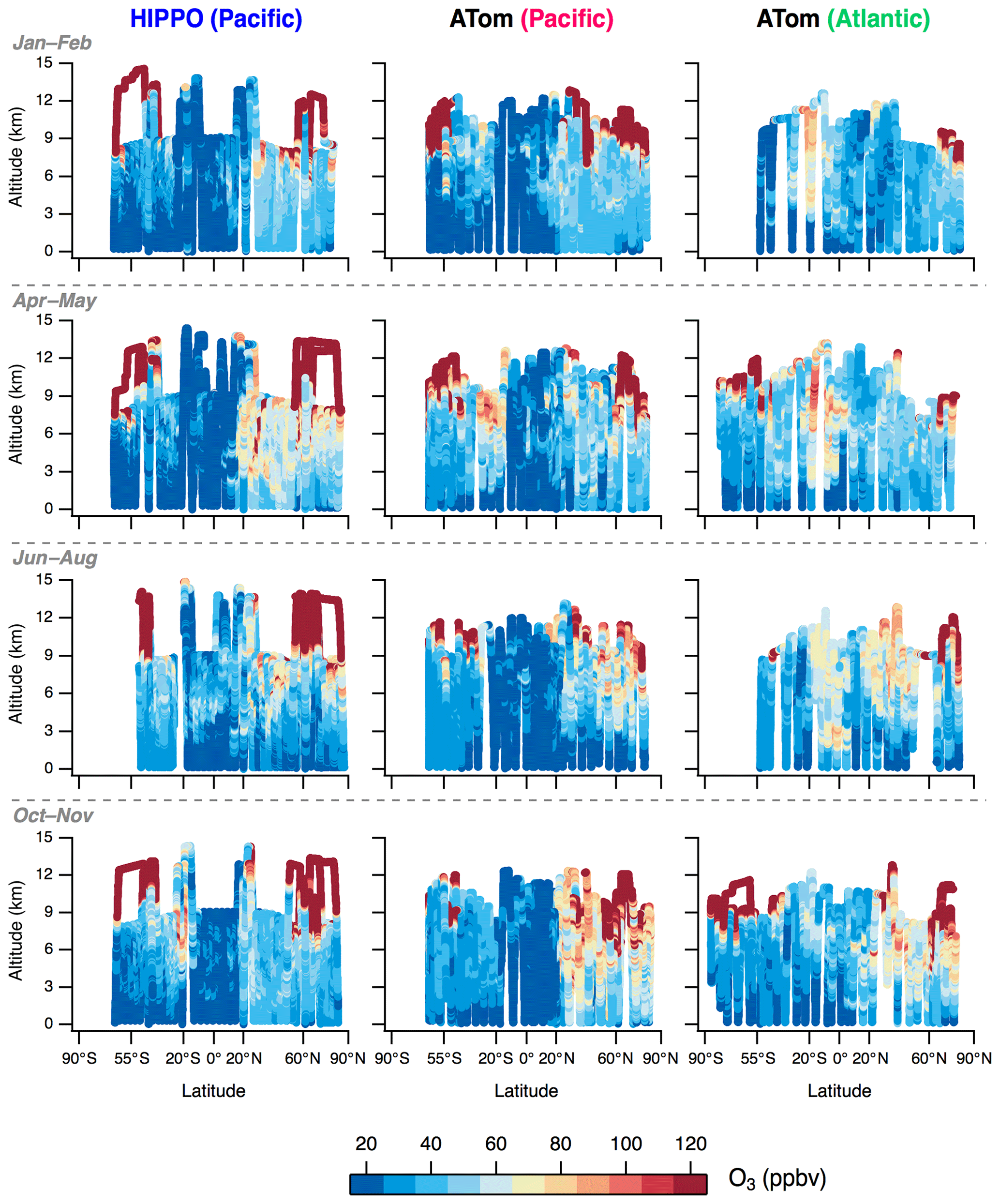
Figure 9 Global-scale distribution of tropospheric O₃ for each ATom and HIPPO seasonal deployment. The rows separate the seasonal deployments, whereas the columns indicate the mission and the ocean basin. The O₃ color scale ranges from 20 to 120 ppbv, and all values outside of this range are shown using the same extremum color (red for values >120 ppbv and blue for values <20 ppbv). HIPPO deployments in June and August were combined.

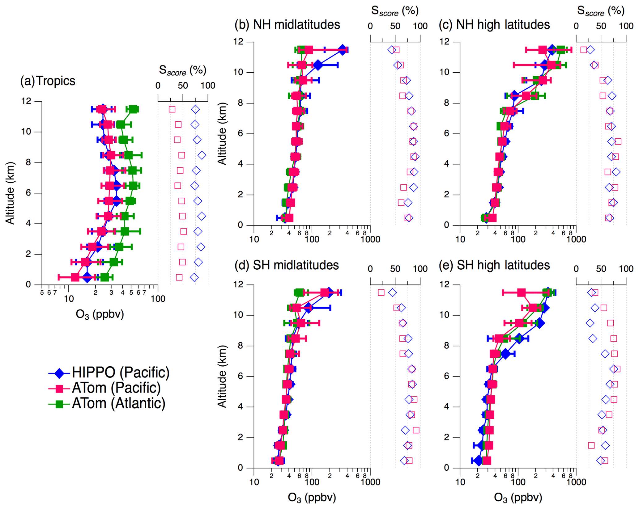
Figure 10 Vertically resolved O₃ distributions from 0 to 12 km are plotted for the Atlantic (ATom in green) and for the Pacific (ATom in pink and HIPPO in blue). The five broad latitude regions correspond to the data parsing illustrated by Fig. 1. Markers indicate median O₃, and bars are the 25th and 75th percentiles, per 1 km altitude bin. Note the log scale on the x axis. S_score values resulting from the comparison of HIPPO and ATom Pacific distributions are shown using blue diamonds, and values resulting from the comparison of ATom Atlantic and Pacific distributions are shown using pink squares.

4.1 Tropics

4.1.1 Vertical distribution

O₃ is at a minimum in the tropical marine boundary layer (MBL), especially over the Pacific (Fig. 10a). The lowest measured O₃ in this region was 5.4 ppbv in May during ATom, and 3.5 ppbv in January during HIPPO. The tropical MBL is a net O₃ sink owing to very slow O₃ production rates – NO levels averaged 22±12 pptv in the Pacific and Atlantic MBL during ATom – and rapid photochemical destruction rates of O₃ in a sunny, humid environment (Kley et al., 1996; Parrish et al., 2016; Thompson et al., 1993). Deep stratospheric intrusions into the Pacific MBL were not observed in ATom or HIPPO, in contrast to reports from previous studies (e.g., Cooper et al., 2005; Nath et al., 2016). In the tropics, marine convection within the intertropical convergence zone (ITCZ) is associated with relatively low O₃ values throughout the tropospheric column, with median O₃ mixing ratios less than 25 ppbv below an altitude of 4 km in the tropical Pacific (Fig. 10a; Oltmans et al., 2001). The relative difference between ATom Atlantic and Pacific median O₃ in the tropics below 8 km is consistently higher than a factor of 1.5, with an average S_score of 43 % (Figs. 10a, 11b). We ascribe this difference to O₃ production from biomass burning (BB) emissions in the continental regions surrounding the tropical Atlantic; back trajectories from the ATom flight tracks show the tropical Atlantic is strongly affected by transport from BB source regions in both Africa and South America (Fig. S4; Jensen et al., 2012; Sauvage et al., 2006; Stauffer et al., 2018; Thompson et al., 2000). In addition, the positive correlation of O₃ enhancements with black carbon (Katich et al., 2018) and reactive nitrogen species (Chelsea Thompson, personal communication, 2017) also indicate BB influence. Although ATom and HIPPO data show evidence of extensive and widespread BB influence on O₃ in the Pacific as well, O₃ mixing ratios are consistently more elevated throughout the tropospheric column in the Atlantic. One reason for this is the closer proximity of the mid-ocean Atlantic flight tracks to O₃ precursor source regions. These findings confirm studies that previously highlighted the impact of African BB emissions on O₃ production in the tropical Atlantic (e.g., Andreae et al., 1994; Fishman et al., 1996; Jourdain et al., 2007; Williams et al., 2010). Lightning NO_x also play a role in the buildup of O₃ over the tropical Atlantic at certain times of year (Moxim and Levy, 2000; Pickering et al., 1996).

4.1.2 Seasonality

The seasonal variation of vertical profiles of O₃ in the tropics is lower throughout the column compared with the extra-tropics (Fig. 12), in part due to less stratospheric influence at the highest tropical altitudes. The remoteness of the tropical Pacific flight paths from continental pollution sources also drives the lower seasonal variability here compared with the tropical Atlantic, where the BB influence peaks in June–August and October–November, characterized by high O₃ (>75 ppbv) and high CO (>100 ppbv) (Fig. 13f), significantly increasing the O₃ vertical distribution compared with the other seasons (Fig. 12c, h, m). Finally, photochemistry, which regulates the O₃ net balance in the troposphere, is less seasonally variable in the tropics than in the extra-tropics, where the photolysis frequency of O₃, j(O₃), and the photochemical production of O₃ fluctuate annually with solar zenith angle.

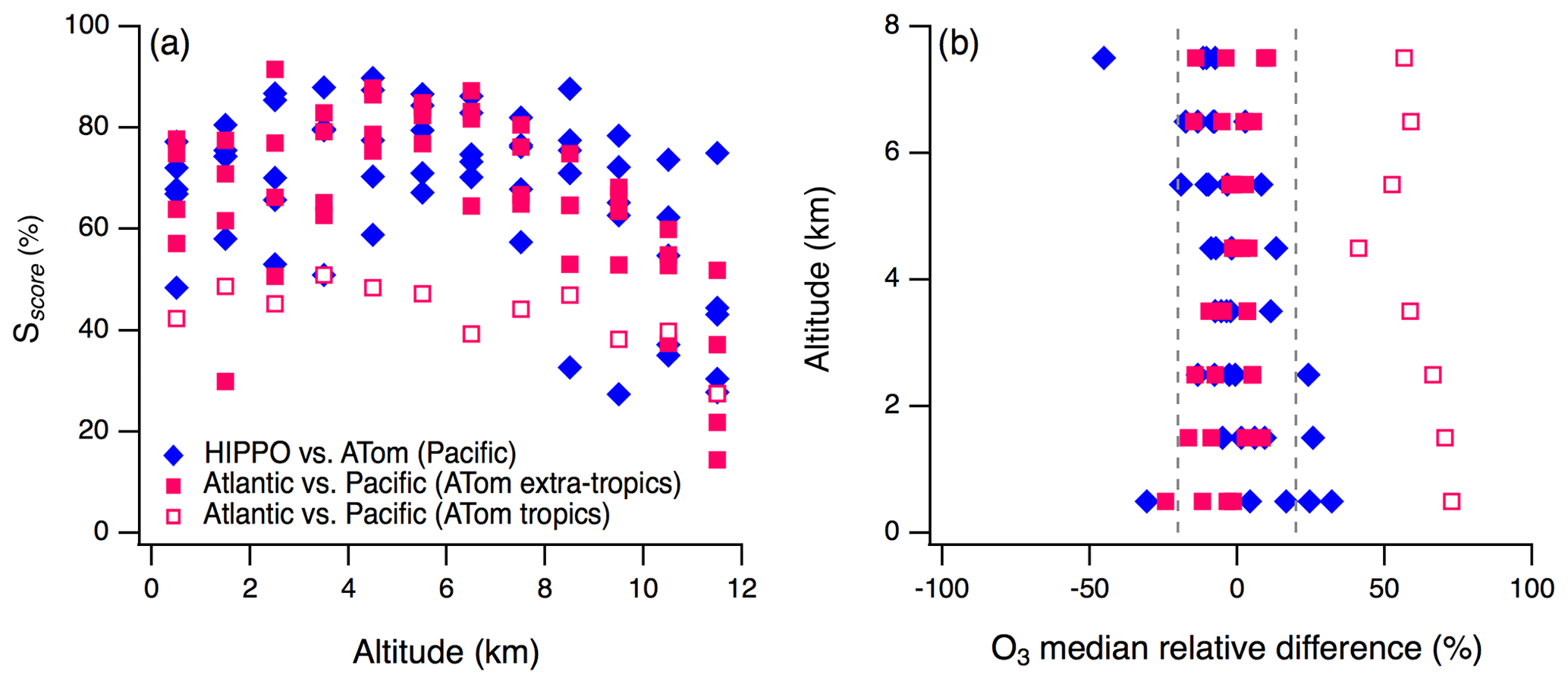
Figure 11 All S_score values from Fig. 10 are shown in panel (a) and are plotted against altitude. The HIPPO and ATom comparison in the Pacific Basin is shown using blue diamonds, and a comparison of the Atlantic and Pacific basins during ATom is shown using filled pink squares for the extra-tropics and open pink squares for the tropics. The relative difference of median O₃ from 0 to 8 km given in Fig. 10 is shown in panel (b), using the same color and marker code as in panel (a). The dotted gray lines indicate a relative difference of 20 %.

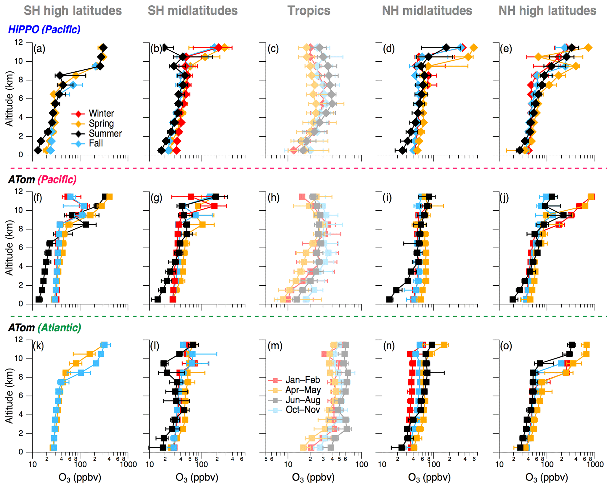
Figure 12 Seasonal variability of the regional O₃ distribution in the Pacific (HIPPO in the top row and ATom in the middle row) and in the Atlantic (ATom in the bottom row). The colors designate the local seasons with red as winter, gold as spring, black as summer, and blue as fall (the corresponding months are indicated for the tropics, using lighter colors). The markers and associated bars correspond to the median, 25th and 75th percentiles, respectively, of the O₃ distribution in every 1 km altitude bin. Note the logarithmic scale on the x axes in all panels and the changing scale with latitudinal bin.

4.1.3 O₃ minima and maxima

Coincident O₃ and CO enhancements were observed in the tropical Atlantic for each ATom circuit (Figs. 9, 13f), suggesting a year-round influence of continental emissions and distinctive dynamics in this region (Krishnamurti et al., 1996; Thompson et al., 1996). In the tropical Pacific, the April–May period stands out due to an O₃ and CO enhancement episode during HIPPO (Fig. 9) that was attributed to the transport of anthropogenic and BB emissions from Southeast Asia (Shen et al., 2014). Deep convection in the tropics brings O₃-poor (<15 ppbv) air to the upper troposphere (Kley et al., 1996; Pan et al., 2015; Solomon et al., 2005). However, the spatial extent of these events remains poorly constrained. Results from ATom and HIPPO suggest that deep convection can loft O₃-poor air at least up to 12 km (the altitude ceiling of this study) in the tropical Pacific and occurred more frequently between January and May (Fig. 12c, h). During the rest of the year, O₃-poor air was typically confined below 4 km. Conversely, O₃-poor air is confined to the first 2 km in the tropical Atlantic (Fig. S5). Meteorological analysis of tropical ozonesondes shows that subsidence of higher-O₃ air aloft over the Atlantic is one reason O₃-poor air is found only in the boundary layer (Thompson et al., 2000, 2012).

4.2 Middle and high latitudes

4.2.1 Vertical distribution

In the middle and high latitudes, tropospheric O₃ was generally at a minimum in the MBL and increased with altitude. Above 8 km, increasing O₃ with altitude (Fig. 10b–e) and its persistent anticorrelation with CO (Fig. 13) points to stratospheric air sampling as the cause for higher O₃ variability in the extra-tropical UTLS, especially at high latitudes where the tropopause is lower and wave breaking of the polar jet streams can lead to stratospheric intrusions. As a result, the S_score decrease above 8 km, summarized in Fig. 11a, is ascribed to variability in the influence of stratospheric air. ATom has detected little change in the O₃ distribution over the Pacific Ocean since HIPPO, with a S_score averaging 74 % in the 0–8 km range. The relative difference between median O₃ values from HIPPO and ATom in the Pacific is generally lower than 20 % (Fig. 11b). Similarly, the relative difference between the median O₃ mixing ratios between ATom Atlantic and Pacific below 8 km is consistently lower than 20 %, with an average S_score of 75 % (Fig. 11b). The southern high latitudes are the only region where the S_score below 8 km occasionally fell below 60 % (Fig. 10e). However, a lower S_score was expected there as the Atlantic vertical profile is based on only two seasonal flights to Antarctica, whereas there were four seasonal flights in the Pacific. Additionally, HIPPO was less spatially extensive – resulting in fewer data points – in this latitude bin compared with ATom (Fig. 1), which could explain the low S_score values when comparing the two missions (Fig. 10e). Nevertheless, the similar O₃ distribution in the extra-tropical free troposphere above the two oceans is consistent with an O₃ lifetime that is sufficiently long for rapid zonal transport to smooth out variations in baseline O₃ distribution in the remote troposphere, across a relatively wide range of longitudes (Fig. 10b–e). The comparison of O₃ seasonal cycles at remote ozonesonde launching sites of the northern midlatitudes yields similar results and further supports this conclusion (Logan, 1985; Parrish et al., 2020). However, the similarity of the O₃ distribution in the extra-tropical free troposphere above the Atlantic and Pacific is not always evident in satellite-, modeling-, or ozonesonde-derived maps (Gaudel et al., 2018; Hu et al., 2017; Ziemke et al., 2017). Additionally, studies of the spatial representativeness of tropospheric O₃ monitoring networks have also concluded that tropospheric O₃ distributions varied significantly with longitude, especially in the northern middle and high latitudes over continents (Liu et al., 2013; Tilmes et al., 2012). In contrast, the ATom findings stem from O₃ measurements predominantly over the oceans, which likely reveal a different picture of O₃ longitudinal distribution away from regional precursor emissions.

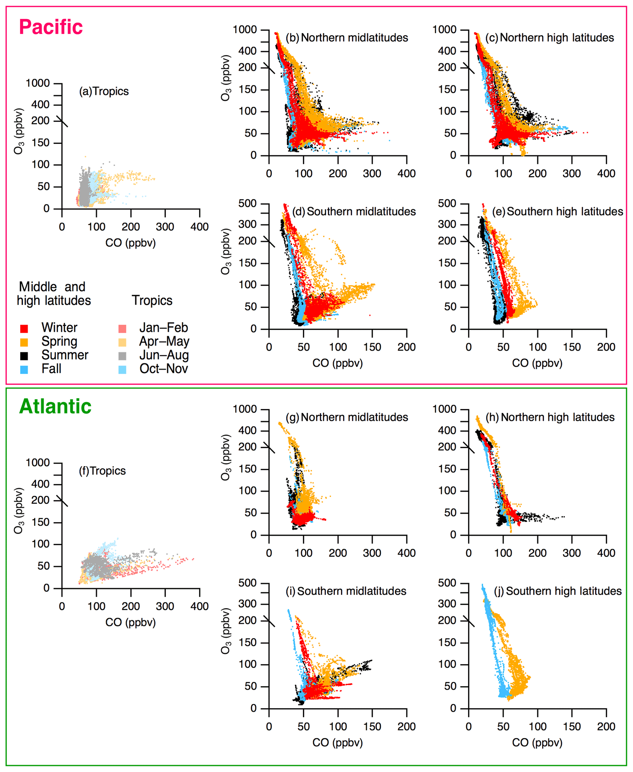
Figure 13 O₃ vs. CO plots using combined ATom and HIPPO data. Each panel denotes a different latitudinal band in each basin. Seasonal deployments are colored according to the legend. Note the logarithmic scale on the y axes in all panels and the changing scale with latitudinal bin.

4.2.2 Seasonality

The extra-tropical vertical profiles of O₃ vary seasonally during ATom and HIPPO. The summer season in the middle and high latitudes was remarkable over both oceans and hemispheres for the steep O₃ gradients in the tropospheric column (Fig. 12 in black). In the MBL, median O₃ was consistently under 25 ppbv in the summer, whereas O₃ was over 25 ppbv in other seasons. Low O₃ in the MBL in summer reflects the enhanced O₃ photochemical destruction in this NO_x-limited region. Photochemical destruction decreases in dry air in the upper troposphere, leading to the steep O₃ gradients observed in this region. The summer O₃ minimum was especially apparent in the high latitudes of the southern Pacific during ATom and extended well above the MBL into the free troposphere (Fig. 12 in black). O₃ mixing ratios were highest in the tropospheric column during springtime in both hemispheres, and over both oceans (Fig. 12 in gold). A notable exception occurred during springtime in the high latitudes of the NH, where several O₃ depletion events were sampled in the lower legs of the Arctic transit. During these events, O₃ mixing ratios lower than 10 ppbv were measured, resulting in a lower 25th percentile of the O₃ distribution at the lowest altitude compared with the other seasons (Fig. 12e and o in gold). A tropospheric O₃ springtime maximum has often been reported in the NH (e.g., Monks, 2000) when meteorology favors efficient transport of O₃ and precursors from continental air from North America and Eurasia (Owen et al., 2006; Zhang et al., 2017, 2008). Another contributing factor is the increased frequency of stratospheric air mixing in spring that significantly contributes to higher O₃ levels (Lin et al., 2015a; Tarasick et al., 2019a). Further, the tropospheric O₃ springtime maximum in the SH is often attributed to BB emissions reaching a peak (Fishman et al., 1991; Gaudel et al., 2018), but stratospheric air mixing also occurs (Diab et al., 1996, 2004; Greenslade et al., 2017). Here, the O₃−CO relationship in spring shows that the enhanced stratospheric mixing with tropospheric air during this season, both in the northern and southern middle and high latitudes, contributes to the increase in column O₃ (Fig. 13). Fall and winter seasons shared similar features in the middle and high latitudes: no strong O₃ gradient was measured in the free troposphere, and O₃ values varied over similar ranges – about 40 ppbv in the NH and about 30 ppbv in the SH – during the two seasons (Fig. 12 in red and blue).

4.2.3 O₃ enhancements

The linear increase of O₃ with CO >100 ppbv highlights the contribution of natural and anthropogenic pollution plumes lofted from continental areas into the remote troposphere. In the NH, these events occur almost year-round (Fig. 13b–c and g–h). Higher CO enhancements in the Pacific (Fig. 13g–h) than in the Atlantic (Fig. 13b–c) have been observed before and have been attributed to sampling bias (Clark et al., 2015). Here, our findings suggest a year-round influence of continental emissions on the Pacific atmosphere despite its remoteness. Modeled back trajectories show that most air masses sampled in the NH during ATom were influenced by long-range transport of continental emissions from Asia, Africa, and North America (Fig. S6). Previous studies have shown that anthropogenic and BB emission outflow from Asia significantly contributed to O₃ pollution events measured over the northern Pacific or in California (e.g., Heald et al., 2003; Jaffe et al., 2004; Lin et al., 2017). Intercontinental transport of anthropogenic emissions from Europe can also contribute to the Asian outflow of anthropogenic pollution (e.g., Bey et al., 2001; Liu et al., 2002; Newell and Evans, 2000). Finally, O₃ enhancements in the northern Atlantic have frequently been observed and have been attributed to midlatitude anthropogenic and boreal forest fire emissions (e.g., Honrath et al., 2004; Martín et al., 2006; Trickl et al., 2003). In the SH, polluted air is encountered more often in spring and summer over the Atlantic, but springtime CO is greater than in other seasons over the Pacific (Fig. 13d–e and i–j). During spring, median O₃ above 50 ppbv was measured throughout the free troposphere in the southern midlatitudes (Fig. 12). Several air masses intercepted during these flights originated from regions that were intensively burning at the time, notably equatorial and southern Africa, Australia, and southern South America, contributing to the observed enhanced O₃ and CO (Fig. S4). Our results expand on previous observation-based but more spatially and temporally limited studies that highlighted co-located enhancements of O₃ and CO at remote locations to show in situ evidence of the frequent, large-scale influence of continental outflow on O₃ in the remote troposphere in both oceans, as well as at almost all latitudes.

5 Conclusions

We present tropospheric O₃ distributions measured over remote regions of the Pacific and Atlantic oceans during two airborne chemical sampling projects: the four deployments of ATom (2016–2018) and the five deployments of HIPPO (2009–2011). The data highlight several regional- and large-scale features of O₃ distributions and provide insight into current O₃ distributions in remote regions. The main findings are as follows:

ATom and HIPPO provide a unique perspective on vertically resolved global baseline O₃ distributions over the Pacific and Atlantic basins and expand upon spatially limited O₃ climatologies from long-term datasets to highlight large-scale features necessary for model output and satellite retrieval validation.

ATom and HIPPO O₃ data are consistent – where they overlap – with measurement-based climatologies of tropospheric O₃ from well-established ozonesonde and commercial aircraft monitoring programs. ATom and HIPPO seasonal median O₃ correlated well with corresponding seasonal median O₃ from ozonesondes (R²>0.7), giving confidence in the accurate depiction of the emerging global O₃ climatology by these diverse research activities. ATom and HIPPO captured 30 %–71 % of O₃ variability measured by ozonesondes launched in the vicinity of the aircraft flight tracks and had the same mode of the O₃ distribution as determined by IAGOS in the northern Atlantic UTLS. This representativeness evaluation on global scales highlights the usefulness of airborne observations to fill in the gaps of established but limited O₃ climatologies. Higher O₃ loading in the NH compared with the SH is consistent with the heterogeneous distribution of O₃ precursor emissions around the globe, mostly concentrated in the NH, which is a result consistent with previous modeling studies and satellite observations. ATom Atlantic vs. Pacific comparison reveals a similar O₃ distribution in the free troposphere up to ∼8 km in the middle and high latitudes, but not in the tropics. Similar O₃ distributions across latitude bands have been suggested in the past, but these studies were limited to the northern midlatitudes. Conversely, other satellite, modeling, and observation-based studies indicated significant O₃ longitudinal gradients. Here, our findings are consistent with zonal transport smoothing the baseline O₃ distribution longitudinally from the Pacific to the Atlantic. In the tropics, median O₃ mixing ratios are about twice as high in the Atlantic as in the Pacific, due to a well-documented mixture of dynamical patterns interacting with the transport of continental air masses.

A comparison of seasonal O₃ vertical profiles did not reveal a marked seasonality in the tropics but instead highlighted the influence of specific events, most notably BB emissions from Africa and South America, which have been extensively documented in the literature. In the extra-tropics, the summer season was characterized by a steeper tropospheric O₃ gradient driven by a very low O₃ abundance in the MBL. Fall and winter seasons generally led to near-constant O₃ mixing ratios from the surface to the upper troposphere, while the highest O₃ abundance was recorded during the spring season when more frequent and intense stratospheric intrusions and transport of air masses from continental regions occur. ATom and HIPPO provide the first airborne in situ vertically resolved O₃ climatology covering both the Atlantic and Pacific oceans in the NH and in the SH. They confirm and extend the current understanding of O₃ variability in the remote troposphere, built over several decades by airborne campaigns, monitoring networks, and satellite observations.

Overall, this paper highlights the value of the ATom and HIPPO datasets, which cover spatial scales commensurate with the grid resolution of current Earth system models and are also useful as a priori estimates for improved retrievals of tropospheric O₃ from satellite remote sensing platforms. In addition, ATom and HIPPO in situ measurements help to establish the quantitative legacy of global pollution transport and chemistry through the evaluation of key, covarying species – in this case O₃ and CO, and reveal the year-round pervasive influence of continental outflow on O₃ enhancements in the remote troposphere. ATom and HIPPO datasets should be critical for improving the scientific community's understanding of O₃ production and loss processes as well as the influence of anthropogenic emissions on baseline O₃ in remote regions. They provide a timely addition to the Tropospheric Ozone Assessment Report (TOAR) effort to characterize the global-scale O₃ distribution and address some of the measurement gaps identified therein.