the Creative Commons Attribution 4.0 License.
the Creative Commons Attribution 4.0 License.
 | 28 Aug 2020
Airborne measurements and large-eddy simulations of small-scale gravity waves at the tropopause inversion layer over Scandinavia
Johannes Wagner
Benjamin Witschas
Coordinated airborne measurements were performed by two research aircraft – Deutsches Zentrum für Luft- und Raumfahrt (DLR) Falcon and High Altitude and Long Range Aircraft (HALO) – in Scandinavia during the GW-LCYCLE II (Investigation of the life cycle of gravity waves) campaign in 2016 to investigate gravity wave processes in the upper troposphere and lower stratosphere (UTLS) region. A mountain wave event was probed over southern Scandinavia on 28 January 2016. The collected dataset constitutes a valuable combination of in situ measurements and horizontal- and altitude-resolved Doppler wind lidar and water vapour measurements with the differential absorption lidar (DIAL). In situ data at different flight altitudes and downward-pointing wind lidar measurements show pronounced changes of the horizontal scales in the vertical velocity field and of the leg-averaged momentum fluxes (MFs) in the UTLS region. The vertical velocity field was dominated by small horizontal scales with a decrease from around 20 to < 10 km in the vicinity of the tropopause inversion layer (TIL). These small scales were also found in the water vapour data and backscatter data of the DIAL. The leg-averaged MF profile determined from the wind lidar data is characterized by a pronounced kink of positive fluxes in the TIL and negative fluxes below. The largest contributions to the MF are from waves with scales > 30 km. The combination of the observations and idealized large-eddy simulations revealed the occurrence of interfacial waves having scales < 10 km on the tropopause inversion during the mountain wave event. The contribution of the interfacial waves to the leg-averaged MF is basically zero due to the phase relationship of their horizontal and vertical velocity perturbations. Interfacial waves have already been observed on boundary-layer inversions but their concept has not been applied to tropopause inversions so far. Our idealized simulations reveal that the TIL affects the vertical trend of leg-averaged MF of mountain waves and that interfacial waves can occur also on tropopause inversions. Our analyses of the horizontal- and altitude-resolved airborne observations confirm that interfacial waves actually do occur in the TIL. As predicted by linear theory, the horizontal scale of those waves is determined by the wind and stability conditions above the inversion. They are found downstream of the main mountain peaks and their MF profile varies around zero and can clearly be distinguished from the MF profile of Kelvin–Helmholtz instability. Further, the idealized large-eddy simulations reveal that the presence of the TIL is crucial in producing this kind of trapped wave at tropopause altitude.
- Article
(12056 KB) - Full-text XML
- BibTeX
- EndNote


Gravity waves (GWs) are an important coupling mechanism between the lower and the middle and upper atmosphere. Propagating GWs transport momentum and energy and deposit them in regions where breaking and dissipation occur. As such, GWs account, for example, for the well-known upper mesospheric wind reversals as well as the cold polar summer mesopause and the warm winter stratopause (Dunkerton, 1978; Lindzen, 1981). So far, different sources for GWs in the troposphere have been identified, e.g. flow over orography, convection, jets and fronts, as well as secondary generation in the region of GW breaking (Smith, 1979; Gill, 1982; Baines, 1995; Fritts and Alexander, 2003; Sutherland, 2010; Plougonven and Zhang, 2014; Vadas et al., 2003). GWs are propagating from their sources in the troposphere and the tropopause region (Sato et al., 2009; Fritts et al., 2016). However, the atmospheric temperature and wind structures influence the propagation of GWs and alter their properties.
Starting with the work of Queney (1948) and Scorer (1949), mountain wave (MW) propagation in the atmosphere was intensively investigated using theoretical and numerical methods. An important and well-known result of these investigations is that the stratospheric solution in a model taking into account a vertically varying background is not dominated by the classical solution of Queney (1948) but by reflected and downstream propagating (trapped) waves in the troposphere (Wurtele et al., 1987; Keller, 1994). The wave spectrum (i.e. wavelengths) is determined by the vertical varying wind and stability and not by the topography spectrum. The topography affects the relative amplitudes (Keller, 1994; Ralph et al., 1997). Fine-scale structures in the atmosphere, such as sharp temperature inversions at the top of the boundary layer (Vosper, 2004; Sachsperger et al., 2015) or in the mesosphere (Fritts et al., 2018), can be wave guides leading to trapped waves which propagate horizontally along the inversions, i.e. interfacial waves. All those findings are in contrast to the fundamental characteristics of the hydrostatic approximation. The fundamental characteristics of the hydrostatic approximation are the absence of a mechanism which allows a wave to propagate horizontally and the consequent upward propagation of energy directly above the obstacle, regardless of the horizontal extent of the generating terrain (Wurtele et al., 1996). Linear non-rotating hydrostatic wave theory is most commonly used by MW parameterizations in weather and climate models to propagate these waves away from the subgrid-scale orography to higher levels (Eckermann et al., 2015).
Currently, much activity using various ground-based, airborne and satellite measurements is going on to get a complete picture of the GW activity and distribution around the globe and to enhance the understanding of source and propagation processes (e.g. Fritts et al., 2016; Podglajen et al., 2016; Wright et al., 2017; Shibuya et al., 2017; Kaifler et al., 2017; Krisch et al., 2017). This knowledge is required to adequately model and parameterize atmospheric GWs in weather and climate models. So far, observational indications of GW behaviour in the tropopause region such as reflection and trapping are rare due to lack of horizontal- and altitude-resolved observations in the tropopause region. Using aircraft measurements, which were taken during the Terrain-Induced Rotor Experiment (T-REX; Grubišić et al., 2008), Smith et al. (2008) were able use in situ data to measure partial reflection of MWs at the tropopause for the first time. Using their linear model, they identified two levels of reflection, one at the altitude where the Scorer parameter, defined as
where N is Brunt–Väisälä frequency, U is the cross-mountain wind speed, z is altitude, and H is scale height (Lane et al., 2000), changes due to changes in static stability, and the other at the altitude with a discontinuity in wind speed but constant Scorer parameter.
In addition, Smith et al. (2008) and Woods and Smith (2010) found signatures of trapped waves with a horizontal wavelength of about 15 km in the in situ measurements in the tropopause inversion layer (TIL) during T-REX. They argue that the Sierra Nevada mountain range is unlikely to be the source of those 15 km waves as such small-scale waves may not reach the tropopause altitude due to the considerable evanescent decay caused by the background conditions. Instead, they suggest that those waves are generated by a nonlinear steepening process. Follow-up model simulations lead to two different explanations. First, the short-wave-like fluctuations observed in the upper troposphere and lower stratosphere (UTLS) region are due to Kelvin–Helmholtz instability along shear lines locally induced by the primary MW; i.e. they are not trapped GWs but instead small-scale wave motions resulting from Kelvin–Helmholtz instability (Mahalov et al., 2011). Second, the downward-propagating GWs, which are created by MW breaking in the middle stratosphere, and their reflection at the tropopause can create a kind of lee wave trapping in the lower stratosphere (Woods and Smith, 2011).
Coordinated airborne measurements were performed by two research aircraft – Deutsches Zentrum für Luft- und Raumfahrt (DLR) Falcon and High Altitude and Long Range Aircraft (HALO) – in Scandinavia during the GW-LCYCLE II (Investigation of the life cycle of gravity waves) campaign in 2016 to investigate GW processes in the UTLS region. A MW event was probed over southern Scandinavia on 28 January 2016. The collected dataset constitutes a valuable combination of in situ measurements and horizontal- and altitude-resolved wind lidar and water vapour lidar measurements in the UTLS. In situ data at different flight altitudes and downward-pointing Doppler wind lidar measurements revealed pronounced changes of the horizontal scales in the vertical velocity field and of the leg-averaged momentum flux (MF) in the UTLS region.
This paper examines the MW case over Scandinavia by means of ECMWF IFS meteorological analyses and the coordinated airborne measurements of the DLR Falcon and HALO which provide horizontal- and altitude-resolved data in the UTLS. The wind data of the downward-pointing Doppler lidar give the opportunity to calculate a continuous profile of MF over a 2 km altitude range in the UTLS. In order to find out what determines the horizontal scales in the vertical velocity field and which process(es) can explain the observed characteristics, we investigate the possible existence of interfacial waves in the TIL (Vosper, 2004; Sachsperger et al., 2015, 2017) similar to their existence on an inversion in the troposphere (Cruette, 1976; Sachsperger et al., 2015; Chouza et al., 2015). The paper is organized as follows. Section 2 describes the models, data and methods used in this paper. Meteorological conditions and observations of the MW event on 28 January 2016 are analysed in Sect. 3.1 and idealized large-eddy simulations of MW propagation in the presence of atmospheric inversions are presented in Sect. 3.2. The results are discussed in Sect. 4, and Sect. 5 concludes the paper.
2.1 ECMWF global analysis
Operational analyses of the ECMWF Integrated Forecast System (IFS) are used to analyse the meteorological conditions on 28 January 2016. These analyses (cycle 41r11) have a horizontal resolution of about 16 km on the reduced linear Gaussian grid (TL1279). The highest of the 137 vertical levels (L137) is located at ∼ 80 km (0.01 hPa). The layer thicknesses gradually increases from ∼ 300 m at ∼ 10 km altitude to ∼ 400 m at ∼ 20 km altitude and ∼ 2 km at ∼60 km altitude2.

Figure 1(a) Topographic map of Scandinavia and area of operation of IOP 6 during the GW-LCYCLE II campaign. The coloured lines indicate Falcon (RF07 and RF08) and HALO (PGS11) flight tracks. The red dots mark the position of Andenes (A), Kiruna (K), Sodankylä (S), Karlstad (Ka) and Stavanger (St). The location of the highest mountain peak on the cross-mountain flight legs is marked with X0. Flight altitudes of Falcon and HALO are shown in panel (b). Falcon flight legs RF07 FL2 and RF08 FL1 and HALO flight legs PGS11 HL1, HL2 and HL4 are cross-mountain flights through X0, which are analysed in this study. Colour shaded areas mark regions covered by the upward-looking HALO water vapour lidar WALES (red) and the downward-looking Falcon Doppler wind lidar in scanning (blue), nadir (green) and flux mode (yellow). The temporal evolution of the ECMWF thermal tropopause height at point X0 is indicated with the thick dashed line.
2.2 Airborne observations
2.2.1 Coordinated research flights on 28 January 2016
The airborne observations took place during Intensive Observation Period 6 (IOP 6) on 28 January 2016 in the framework of the combined missions POLSTRACC (The Polar Stratosphere in a Changing Climate), GW-LCYCLE II and SALSA (Seasonality of Air mass transport and origin in the Lowermost Stratosphere using the HALO Aircraft). An overview of the performed HALO research flights can be found in Oelhaf et al. (2019). In January 2016, the DLR Falcon and HALO operated from the airport of Kiruna (67.82∘ N, 20.33∘ E), northern Sweden, to investigate chemical and dynamical processes in the UTLS region at high latitudes. The goal of IOP 6 was to measure a transient MW event over southern Scandinavia with coordinated cross-mountain flights of both aircraft. Figure 1a shows the operational area and the flight tracks of the research flights. The mountains were crossed at the same latitude two times by the DLR Falcon (flight legs RF07 FL2 and RF08 FL1) and three times by HALO (flight legs HL1, HL2 and HL4; Fig. 1b). The limited range of the DLR Falcon required a refuel stop at Karlstad airport. The DLR Falcon was flying close to the thermal tropopause on all flight legs and measured vertical winds and GW-induced momentum fluxes with the in situ sensor at flight altitude and with the downward-pointing Doppler wind lidar below the aircraft. On the flight legs HL1 and HL2, HALO was flying in the troposphere (HL1 below the DLR Falcon) and measured wave structures at flight level and in the tropopause region with the upward-pointing differential absorption lidar (DIAL) measuring water vapour concentration and backscatter (WALES) (Wirth et al., 2009).
2.2.2 Wind lidar measurements
The DLR Falcon was among others equipped with a downward-looking coherent Doppler wind lidar (DWL) which has been operated by DLR since 1999 and which has been applied in a number of field campaigns (e.g. Chouza et al., 2017; Schäfler et al., 2018; Marksteiner et al., 2018; Lux et al., 2018). The DWL operates at a wavelength of 2 µm and is equipped with a double-wedge scanner which enables to steer the laser beam to any position within a cone angle of 30∘. A more detailed description of the 2 µm DWL instrumental setup, the measurement principle, the applied retrieval algorithms and the accuracy and precision of the derived wind products is given by Chouza et al. (2015), Witschas et al. (2017) and more recently Witschas et al. (2020a).
Usually, the 2 µm DWL is used to either measure the three dimensional wind vector by applying the velocity azimuth display (VAD) scan technique, or to measure vertical wind speeds by pointing the laser beam to nadir direction and compensate any attitude changes of the aircraft by means of the double wedge scanner. As shown and discussed by Witschas et al. (2017), measurements of both horizontal and vertical wind profiles are very useful to characterize the spectral properties of MWs. In order to additionally gain knowledge of the momentum transport of MWs, horizontal wind speed (u) and vertical wind speed (w) need to be measured simultaneously. For this purpose, the 2 µm DWL has been operated with a modified scan pattern during the GW-LCYCLE II campaign for the first time. In particular, the laser beam has alternately been steered forth and back with an off-nadir angle of ±20∘. With that and the knowledge of the laser beam pointing direction, u and w can be derived from a successive pair of line-of-sight (LOS) measurements. It is worth mentioning that u denotes the horizontal wind along flight direction here, which coincided well with the wind direction for the discussed flight (see Sect. 3.1.1). The leg-averaged momentum flux () can then be calculated (Smith et al., 2016). Here, ′ denotes perturbations of the respective quantity. In our analysis, we use spectral filters, namely Butterworth, to determine u′ and w′ for different wave classes (i.e. long, intermediate and short waves) as it was done by Georgelin and Lott (2001). We separate the wave classes based on the dominant horizontal wavelengths occurring in the wavelet power spectra, i.e. long (> 30 km), intermediate (10 to 30 km) and short (< 10 km) waves (Sect. 3.1.2). For these three wave classes, the averaged MF and the corresponding uncertainty is computed. In particular, a thousand sub-legs are created as such that their start (end) point is fixed at the westernmost (easternmost) point of the measurements and the length of the leg is stepwise extended eastward (westward) by 1 km starting with a minimum length of 200 km and going up to 700 km, i.e. the full leg length. This is done to incorporate the sensitivity of the leg-averaged MF with respect to the start/end points of the leg and the corresponding unequal sampling of updrafts and downdrafts as already suggested and analysed in a similar way by Brown (1983). We additionally found differences in the MF from DWL and HALO in situ data at 7.8 km altitude, although one hardly can determine differences in u and w between DWL and HALO in situ data. In particular, the difference in w is 0.0±0.2 m s−1 on average. In the end, the given standard deviation accounts for these uncertainties in the MF profile being a worst-case estimate with sub-legs included which have lengths shorter than λMAX∕2 with theoretically λMAX≈700 km for the discussed measurement flight.
For the applied scan pattern, each LOS measurement took 2 s and the aircraft speed above ground was approximately 200 m s−1. Thus, the horizontal resolution of the measured horizontal and vertical wind is ≈ 800 m. A more detailed explanation of the momentum-flux scan pattern of the 2 µm DWL will be presented in Witschas et al. (2020b).
2.2.3 In situ measurements
Horizontal and vertical velocity data at flight level are provided by the DLR Flight Experiments facility. For the DLR Falcon, the velocity field is determined from data taken by a Rosemount model 858 flow angle sensor and a Honeywell Lasernav YG 1779 inertial reference system (IRS) (Bögel and Baumann, 1991). Measurements on HALO are conducted by the Basic HALO Measurement and Sensor System (BAHAMAS). Recent method and calibration details can be found in Mallaun et al. (2015) and Giez et al. (2017). For the horizontal wind, the measurement uncertainties are smaller than 0.5 m s−1 for HALO and 0.9 m s−1 for Falcon, and smaller than 0.3 m s−1 for the vertical wind (Heller et al., 2017; Bramberger et al., 2018). The data are used at a time resolution of 1 s. Perturbation quantities of the velocity data (u′, v′, w′) for the full-leg analysis are calculated by de-trending the data with a linear least-square fit and subtracting the mean over the leg (Portele et al., 2018). Wavelet spectra of vertical velocity and MF cospectra of (Woods and Smith, 2010) with modifications of Portele et al. (2018) are computed based on Torrence and Compo (1998)3. When combining the MF estimates of DWL and in situ data, in situ horizontal velocity along flight direction is used, and u′ and w′ for the three wave classes are determined and analysed in the same way as described in Sect. 2.2.2.
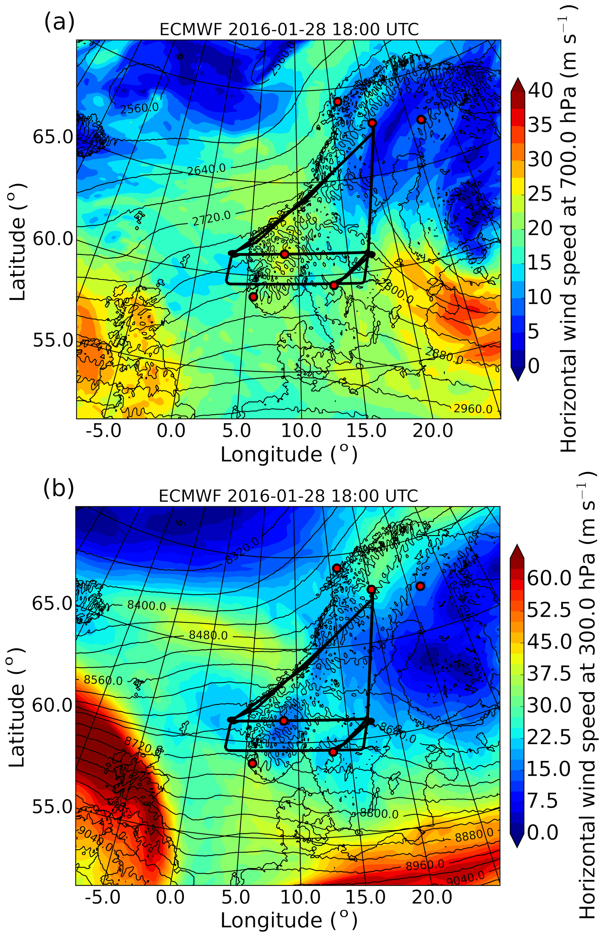
Figure 2Meteorological maps of horizontal wind speed and geopotential height (black contour lines) at (a) 700 hPa and (b) 300 hPa at 18:00 UTC on 28 January 2016 obtained from the ECMWF model. Black lines indicate flight legs of the three research flights and red dots mark the same locations as in Fig. 1.
2.3 Idealized numerical simulations
EULAG4 is a multi-scale computational model for the simulation of geophysical flows. It provides at least second-order accuracy in time and space (Prusa et al., 2008). EULAG solves the governing equations of motion either in an EUlerian or a LAGrangian form. Here, the non-hydrostatic equations of motion,
are used in their Boussinesq approximated ( kg m−3) form for the first set of simulations and decrease of density with altitude () is taken into account for the second set of simulations (Smolarkiewicz et al., 2001; Prusa et al., 2008). is the material derivative, v is the velocity vector, p is pressure, ρ is density, θ is potential temperature, ℳ represents appropriate metric forces, f and g symbolize the vectors of Coriolis parameter and gravity acceleration, z is altitude, and H is scale height. Primes denote deviations from the ambient state and overbars refer to the horizontally homogeneous hydrostatic reference state of the Boussinesq expansion around a constant stability profile (Smolarkiewicz et al., 2001). EULAG has been applied for a broad range of topics in fluid dynamics including orographic GWs (e.g. Prusa et al., 1996; Grubišić and Smolarkiewicz, 1997). The detailed model setup is given in Sect. 3.2.
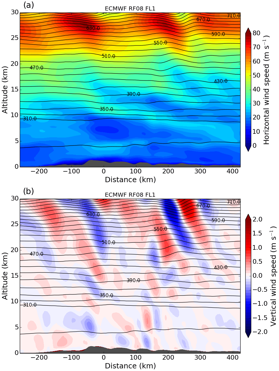
Figure 3ECMWF vertical cross sections of (a) horizontal wind speed and (b) vertical wind speed interpolated in time and horizontal space along flight leg RF08 FL1. Black contour lines indicate potential temperature with an interval of 20 K. The cross-section distance is centred at X0 (see Fig. 1).
3.1 MW event over southern Scandinavia
3.1.1 Meteorological situation
IOP 6 was a transient MW event over southern Scandinavia on 28 January 2016. Two synoptic low-pressure systems over the tip of Greenland and over the Baltic Sea caused moderate southwesterly to westerly winds (10 to 20 m s−1) in the troposphere and the excitation of MWs at the southern Scandinavian mountain range (Fig. 2a). At tropopause level (300 hPa) winds were westerly and below 30 m s−1 over southern Scandinavia as the polar front jet was located over the British Isles and northern Germany. A secondary jet streak occurred over the Norwegian Sea between Iceland and the Norwegian coast (Fig. 2b). The vertical cross section of horizontal wind speed interpolated in time and space along flight leg RF08 FL1 shows increasing wind speed up to 80 m s−1 above 20 km altitude in the stratosphere (Fig. 3a). The cross section of vertical wind shows vertically propagating MWs in the troposphere and increasing wave amplitudes in the stratosphere (Fig. 3b). The resolved MWs in ECMWF are associated with the main mountain peaks of the IFS model topography.
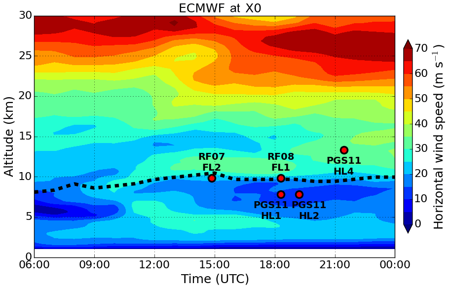
Figure 4ECMWF time–height section of horizontal wind speed at point X0. The dashed black line marks the height of the thermal tropopause. Red dots mark the altitudes of HALO and Falcon at point X0 of the respective flight legs (see also Fig. 1).
In Fig. 4, a time–height section of ECMWF horizontal wind speed located at the mountain ridge at point X0 (Fig. 1a) is plotted. MWs were generated by moderate wind speeds in the lower troposphere on 28 January 2016. However, the MWs were prevented from propagating into the stratosphere until about 08:00 UTC due to weak winds close to 0 m s−1 in the mid-troposphere. After 10:00 UTC, wind speeds above the tropopause and in the mid-troposphere increased which have allowed vertical propagation of tropospheric GWs into the stratosphere. During the time of the research flights (red dots in Fig. 4), wind speeds below the tropopause weakened again (10–15 m s−1).
Vertical profiles of horizontal wind speed and Brunt–Väisälä frequency from an operational sounding5 started from Stavanger (Fig. 1) at 12:00 UTC on 28 January 2016 are shown in Fig. 5a, b. This figure illustrates the moderate winds in the troposphere, the pronounced jump in static stability at the tropopause, which is typical for a TIL (Birner, 2006), and the increasing winds with height in the stratosphere within the polar vortex. The critical horizontal wavelength () which separates evanescent and propagating GWs was mainly larger than 10 km in the troposphere (i.e. only waves with horizontal wavelength > 10 km can propagate), smaller than 10 km in the vicinity of the TIL and increasing towards 20 km above in the stratosphere (Fig. 5d).
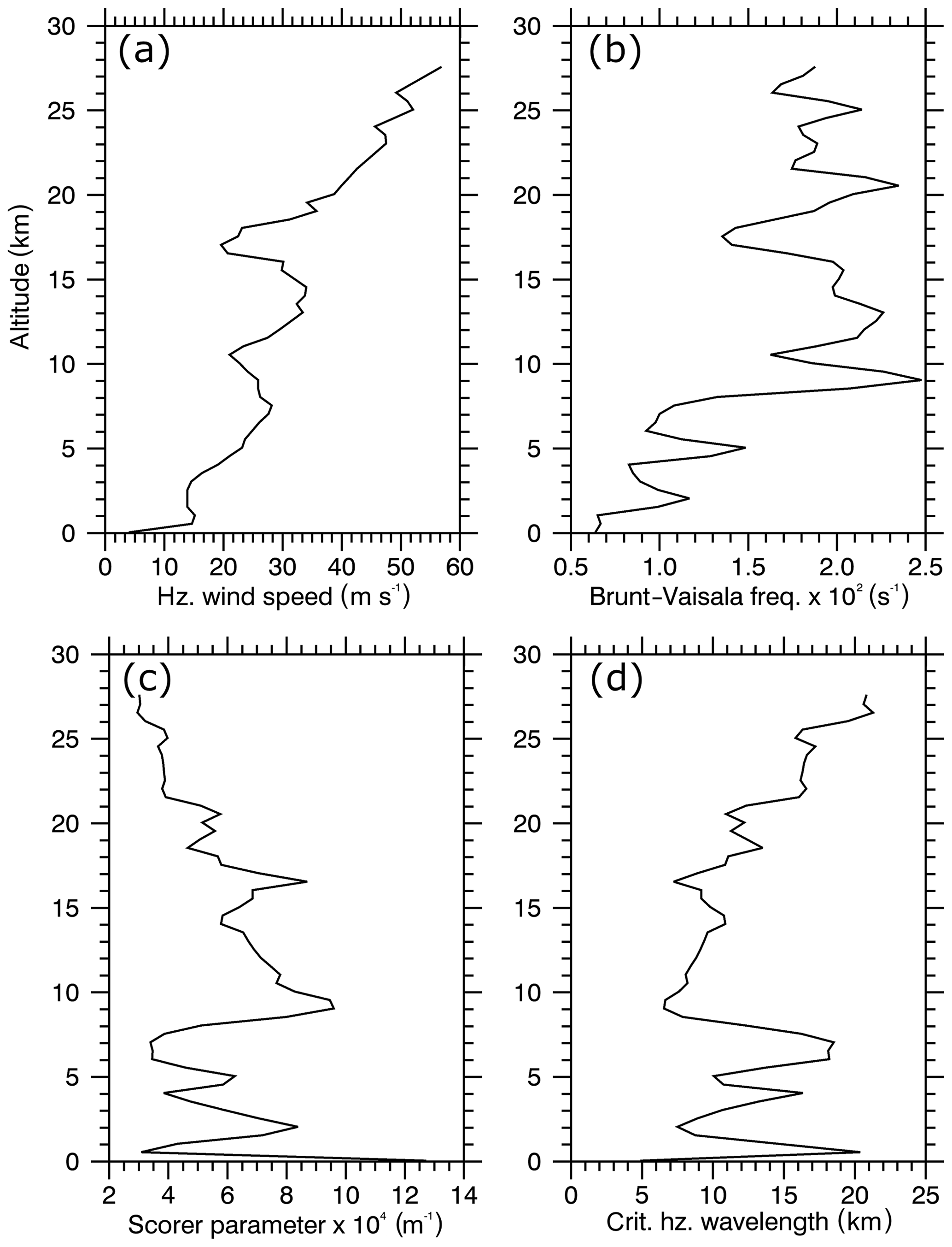
Figure 5Vertical profiles of (a) horizontal wind speed, (b) Brunt–Väisälä frequency, (c) Scorer parameter and (d) critical horizontal wavelength of the radiosonde launched at Stavanger (St) in southern Norway (Fig. 1) at 12:00 UTC on 28 January.
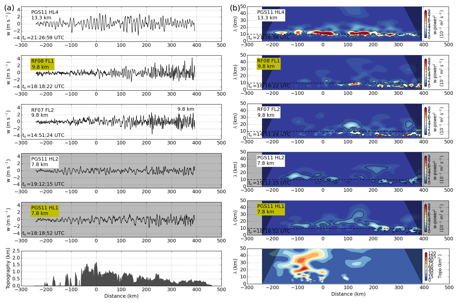
Figure 6Cross-mountain flight legs of Falcon and HALO for panel (a) in situ vertical wind and topography and (b) corresponding wavelets with the horizontal wavelength given on the y axis. The dashed horizontal line marks 10 km horizontal wavelength that separates short and intermediate scale waves. Black contour lines mark regions significant at the 95 % confidence level. The cone of influence is shaded in grey. Flight legs located below the tropopause (see labelled mean flight altitudes) are marked with grey background colour. Time t0 indicates when the aircraft was located at X0 (see Fig. 1) and shows that PGS11 HL1 and RF08 FL1 (labelled with yellow boxes) took place nearly at the same time (HALO was flying 30 s behind Falcon).
3.1.2 Airborne observations
The coordinated flights of HALO and DLR Falcon provided simultaneous measurements of GW-induced perturbations below and in the TIL. Figure 6a shows vertical velocities observed at flight level on all five cross-mountain flight legs. Amplitudes of 2 m s−1 in the troposphere and up to 4 m s−1 in the stratosphere are visible on all legs. Tropospheric measurements (HL1, HL2) show longer horizontal wavelengths compared to the observations at tropopause altitudes (RF07 FL2, RF08 FL1), which means that GW properties change in the vicinity of the tropopause. Wavelet power spectra of the observed vertical winds were computed to analyse the change in horizontal wavelengths (Fig. 6b). Wavelengths in the troposphere were in the order of 10 to 30 km (PGS11 HL1 and HL2), while wavelet analysis shows that shorter wavelengths of 5 to 9 km are dominating the vertical velocity of RF07 FL2 and RF08 FL1 in downstream region. Longer waves with wavelengths of ≥ 10 km are found for the uppermost flight leg in the lower stratosphere (PGS11 HL4). Note that this was the last flight leg and it took place about 2 h later than the other flight legs. The revealed wave signatures are not directly related to the topography spectrum (Fig. 6b) which was computed from the ASTER topography data (Schmugge et al., 2003) along the flight track (shown in Fig. 6a). The wave signatures are influenced by the background conditions.
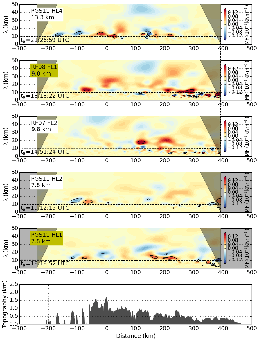
Wavelet cospectra of MF were computed to study the propagation characteristics of the waves in more detail (Fig. 7). Alternating positive and negative MF at wavelengths of 10 to 30 km were observed at distances of −100 to 0 km and 100 to 300 km below and in the tropopause region on the flight legs which took place at nearly the same time (PGS11 HL1 and HL2, RF08 FL1). This alternating pattern is an indication for reflected and trapped waves (Woods and Smith, 2010, see also Sect. 3.2). Significant MF at shorter wavelengths is found in the tropopause region and strongest alternating positive and negative signals occur downstream of the main mountain peaks. No significant positive or negative MF is found for the short scales < 10 km above the tropopause at 13 km altitude (PGS11 HL4). These findings indicate that the short waves are trapped in the tropopause region. Upward-propagating longer waves (negative MF) with horizontal wavelengths of approximately 40 to 50 km are found for RF08 FL1 and PGS11 HL4 at 120 km distance. Positive MF for the long waves is found in RF08 FL1 at 220 km distance which could be caused by partial reflection of these waves. Based on the wavelet spectra, three wave classes can be distinguished according to their horizontal scales: long (> 30 km), intermediate (10 to 30 km) and short (< 10 km) waves.
The DLR Falcon DWL measured in nadir mode on the first cross-mountain flight leg RF07 FL2 (Fig. 8). Measured vertical winds show fine-scale up- and downdrafts over the mountains. The horizontal wavelengths of the GWs are smaller downstream of X0 on the lee side of the mountain and the phase lines are vertical. This again indicates wave trapping.
Lidar and in situ measurements of the coordinated flight legs RF08 FL1 and PGS11 HL1 are shown in Fig. 9. As the DWL operated in flux mode on this leg, both the horizontal wind component in flight direction and the vertical wind component were measured. Contour lines of lidar measurements are overlaid by in situ wind measurements of both aircraft. Wind measurements are complemented by water vapour measurements of the upward-looking DIAL aboard HALO. Horizontal wind speeds in Fig. 9a show large-scale wave structures with upstream tilted phase lines in the troposphere. In situ measurements around the tropopause indicate similar wave structures but with stronger wind speeds compared to tropospheric values. In addition, large-scale wave structures are superimposed by small-scale waves with vertical phase lines. These small-scale waves are more clearly visible in vertical wind measurements, which are more sensitive to smaller-scale waves (Lane et al., 2003; Smith and Kruse, 2017) and show a clear change from intermediate to smaller wavelengths below and in the vicinity of the tropopause (Figs. 8 and 9b). This behaviour was already revealed by the wavelet analysis of the in situ measurements (Fig. 6b). The short horizontal wavelengths are also visible in observations of water vapour mixing ratio (Fig. 9c) and the lidar backscatter ratio at 1064 nm (Fig. 9d) between 8 and 10 km altitude. A backscatter ratio > 1 in the DIAL data reveals the presence of aerosols and clouds.
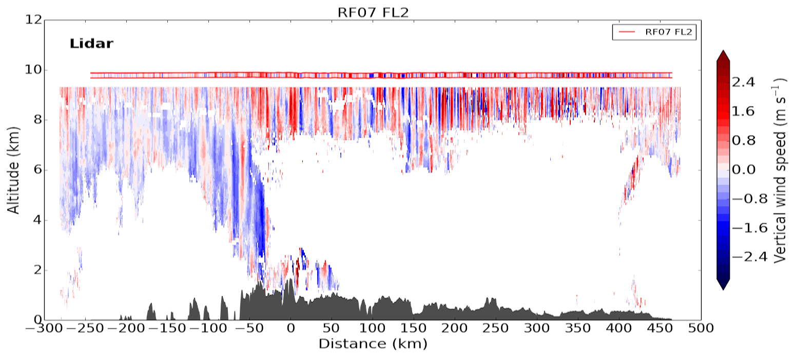
Figure 8Vertical winds along flight leg RF07 FL2 measured by the DWL and in situ instruments (marked by horizontal red lines) at flight level by the DLR Falcon.
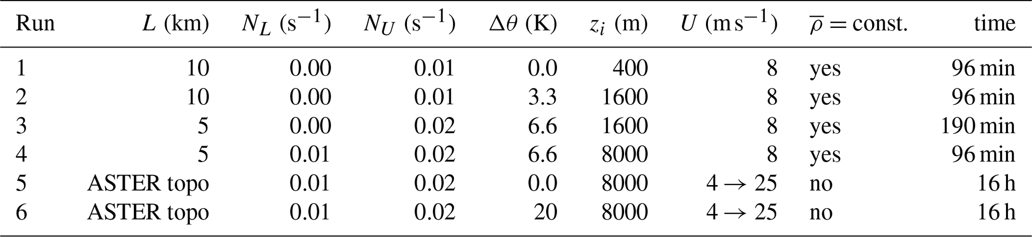
Table 1Mountain width L, static stabilities of the lower and upper layers (NL, NU), strength of the inversion (Δθ) and inversion height (zi), upstream wind conditions, background density and integration time of the EULAG simulations.
Additional information regarding the wave propagation comes with the direct measurements of GW-induced momentum fluxes by the new momentum-flux method of the Falcon DWL. This was done on the coordinated flight leg RF08 FL1. Figure 10 illustrates vertical profiles of leg-averaged momentum fluxes along the cross-mountain flight legs RF08 FL1, PGS11 HL1 and HL4 obtained from lidar and in situ measurements. The MF profiles can be distinguished for the three wave classes defined above. The most prominent feature is the kink reaching positive values for the long waves between 8 and 9 km altitude. Negative fluxes of the same magnitude are found below. This strengthens the previous assumption that waves are partially reflected at the TIL. The mean MF at 7.8 km altitude of the DWL and the HALO in situ data differs but within the range of uncertainty. It is worth mentioning that the uncertainty in the MF from the in situ data is largest at this altitude and larger than the uncertainty derived for the DWL data. This means the MF from in situ data at this altitude could be biased to MF of larger magnitude due to localized peaks in along the leg. The intermediate- and short-scale waves show similar MF profiles with small undulations around zero. The leg-averaged momentum flux of the long waves is positive (around −0.05 Pa) at 13.3 km altitude which could be a hint for wave reflection in the stratosphere or a stratospheric source creating downward-propagating GWs.
3.2 Idealized simulations of MWs and the TIL
In this section, it is investigated if interfacial waves on an inversion found in the lower troposphere can also occur at tropopause altitudes and which conditions are necessary for their occurrence. It is tested if this wave trapping was possible on 28 January 2016 over southern Scandinavia by performing additional two-dimensional simulations with the Scandinavian topography and background profiles which approximate the prevailing conditions on that day. There is no intention to tune the simulations as close to the measurements as possible because the main goal in this study is to identify processes which could explain the observed wave structure in the UTLS.
The computational parameters are chosen similar to Vosper (2004) for the first set of simulations. The two-dimensional domain consists of 1032 and 2000 grid points in x and z directions, respectively, with grid increments of Δx = 100 m and Δz = 10 m (terrain following). This results in a total domain size of about 103 km × 20 km. Open boundaries are applied in the x direction. The model top is a rigid lid. The sponge layers at the horizontal edges of the domain are 8 km wide and the sponge layer at the top of the domain starts at 15 km altitude. As in Vosper (2004), an idealized ridge,
where , and a free-slip lower boundary condition is used. Mountain height h0 is set to 400 m and width L to 10 km or 5 km. The usage of this idealized ridge is considered to be sufficient to investigate the occurrence and changes in the horizontal scale of the GWs in the vicinity of the TIL because it is known that the horizontal wavelength of interfacial waves is independent of the mountain half-width and height (Sachsperger et al., 2017). Four simulations are performed with a vertically constant horizontal velocity U=8 m s−1 and different profiles of potential temperature with the corresponding Brunt–Väisälä frequency as initial conditions. The integration time step Δt is set to 1 s. The total integration time for these simulations is between 96 and 190 min. The initial disturbance created by the mountain during the initialization of the simulations has moved far enough downstream in the region of interest and the simulations have reached quasi-steady state by that time. Table 1 summarizes the relevant initial parameters and total integration time for the different model runs.
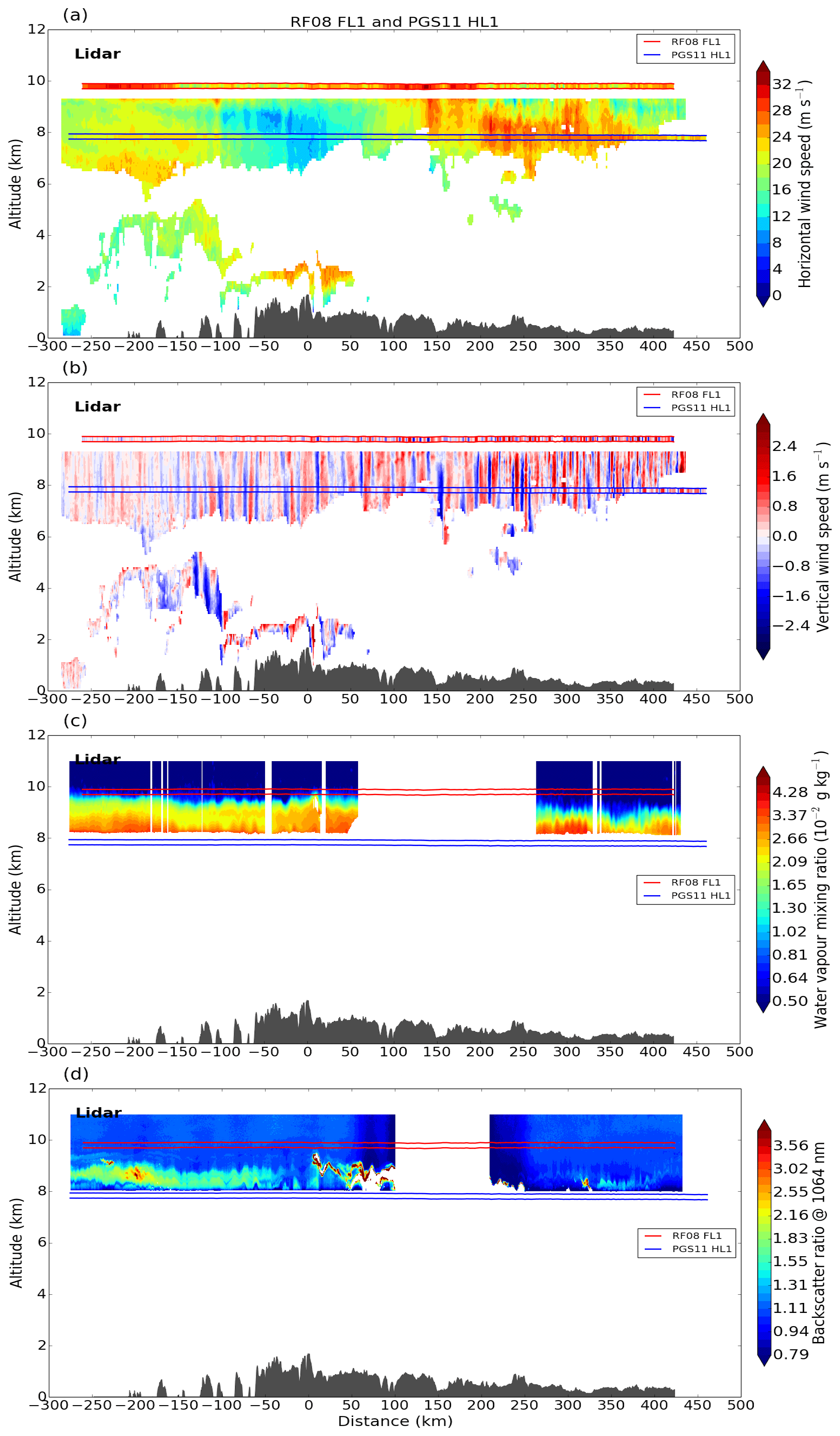
Figure 9DWL measurements of (a) horizontal wind speed and (b) vertical wind speed and WALES measurements of (c) water vapour mixing ratio and (d) lidar backscatter ratio along flight leg RF08 FL1/PGS11 HL1 combined with corresponding in situ measurements of HALO and DLR Falcon at flight level (marked by horizontal blue and red lines).
Figure 11a, b (runs 1 and 2) show that the EULAG model can reproduce the findings of Vosper (2004): an inversion at the top of a neutral boundary layer leads to downstream propagating waves at the altitude of the inversion (Fig. 11b). The horizontal wavelength is approximately 5 km and the largest amplitudes are found in the vicinity of the inversion (Fig. 12c). The signal downstream of the terrain is weak below the inversion (Fig. 12d) and absent if no inversion is present (Fig. 12a, b). If the stability above the inversion is increased to NU=0.02 s−1 (stratospheric stability), the strength of the inversion Δθ must be twice as large to allow for wave trapping and horizontal propagation on the inversion (run 3). The horizontal wavelength of the interfacial waves decreases with increasing stability above the inversion. The horizontal wavelength is approximately 2.5 km for U=8 m s−1 and NU=0.02 s−1 (Fig. 12f). This is because for NU=0.02 s−1 waves with a horizontal wavelength of 5 km are no longer evanescent above the inversion and can propagate vertically (no trapping).
For run 2, wave classes can be defined according to their horizontal scales, i.e. > 6 km for intermediate MWs and <6 km for short waves. Figure 13 shows the MF (profiles) for the two wave classes. In Fig. 13b, it can be seen that the short wave class not only contains interfacial waves but also some upward-propagating non-hydrostatic MWs that are close to the mountain at low levels and propagating further downstream at higher levels. When MF is averaged for the whole domain, the MF profiles of the intermediate and the short waves show a distinctive kink at the altitude of the inversion (Fig. 13e). This is not found when the inversion is absent (Fig. 13a). When MF is averaged for the downstream region, the resulting MF of the interfacial waves depends on the exact start/end points of the downstream region with respect to the wave phase. This is because the interfacial waves show alternating positive and negative fluxes downstream of the mountain (Fig. 13b). In contrast to upward-propagating mountain waves (Fig. 13d), the phase shift between u′ and w′ is −90∘ for interfacial waves below the inversion (Fig. 13c) and changes to +90∘ right above the inversion (not shown). When MF is averaged over a downstream region that only contains full wave cycles, the resulting MF is zero for well-established and totally trapped interfacial waves (Fig. 13e). When the start/end points of the downstream region are chosen such that waves are partly included, MF can be negative (positive) right below the inversion and positive (negative) above the inversion. The sign of MF depends on the cutting location in the wave cycles; i.e. it depends on if more negative (positive) MF is included in the average (Fig. 13b). This MF profile of the interfacial waves differs from the MF profile of Kelvin–Helmholtz instability for which MF is zero below and above the instability (Mahalov et al., 2011).
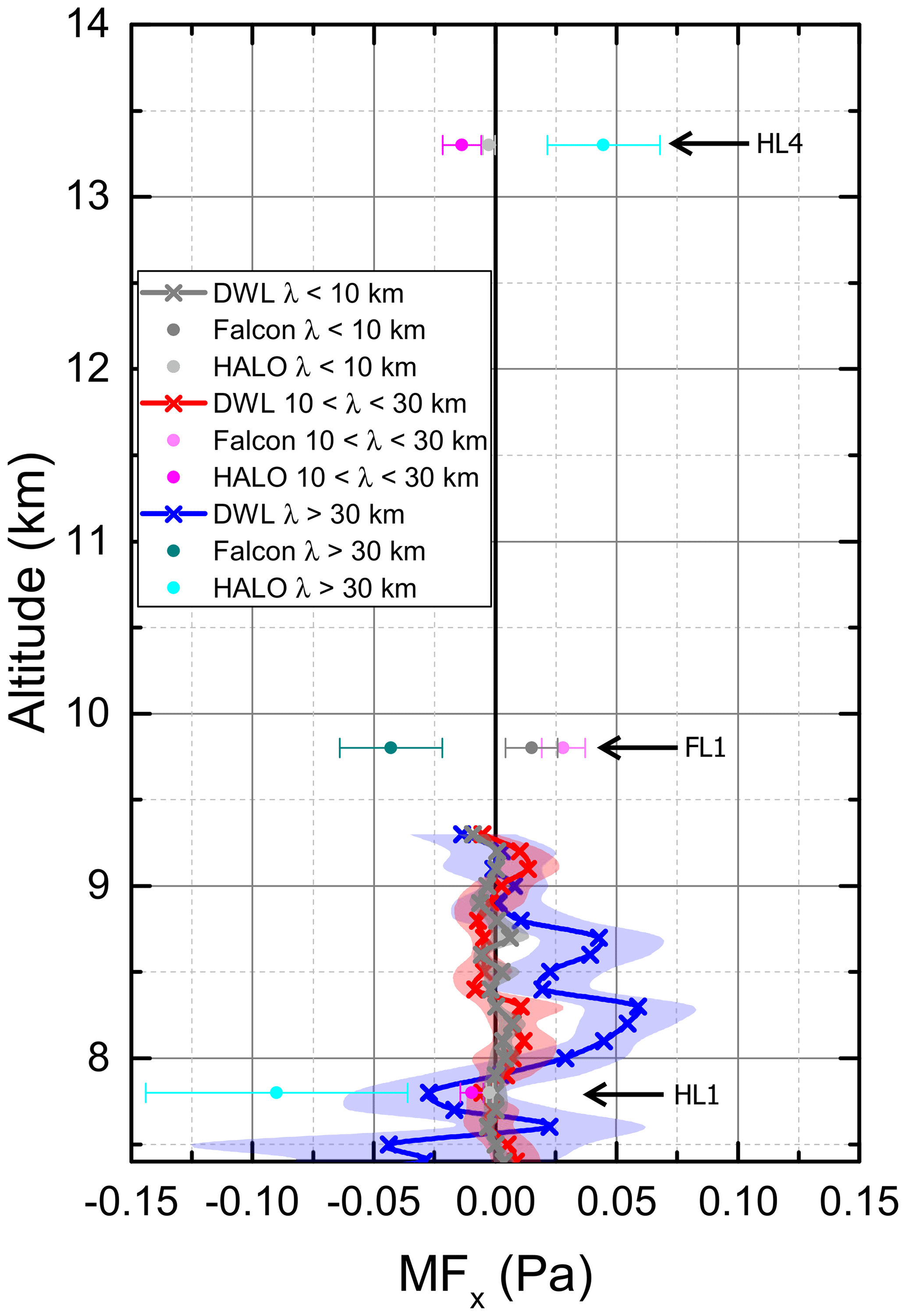
Figure 10Leg-averaged momentum fluxes as mean for varying leg length (solid) with standard deviation (shading, error bars) along flight leg RF08 FL1 obtained from DWL (×) and in situ measurements (•) which include also PGS11 HL1 and HL4. Three wave classes are colour coded and bold black line separates positive and negative fluxes.
Figures 11d and 12h (run 4) show that interfacial waves can also exist in the TIL located between a stably stratified troposphere (NL=0.01 s−1) and the stratosphere (NU=0.02 s−1). The horizontal wavelength is again approximately 2.5 km for U=8 m s−1. Besides the upward-propagating MWs and the interfacial waves, reflected waves with a horizontal wavelength of approximately 5 km exist downstream of the mountain in the troposphere (Figs. 11d and 12j) although the classical trapping condition of a decreasing Scorer parameter with altitude in the troposphere (Scorer, 1949) is not fulfilled. The amplitudes of the reflected waves in the troposphere are found to be larger if an inversion is present at the tropopause than if there is just the jump from tropospheric to stratospheric stability (not shown). The results of these numerical simulations confirm that interfacial waves can exist in the TIL. The mechanism of their trapping (evanescence in the layer above the inversion), the resulting horizontal wavelength and the occurring horizontal propagation match the published results for boundary-layer inversions (Vosper, 2004; Sachsperger et al., 2015).
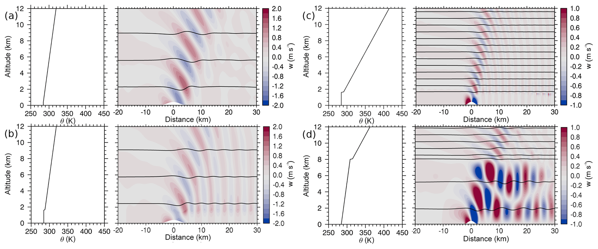
Figure 11Potential temperature and vertical velocity of the idealized simulations of the cases with (a) a neutral boundary layer without inversion and NU=0.01 s−1 (run 1), (b) a neutral boundary layer with an inversion of 3.3 K and NU=0.01 s−1 (run 2), (c) a neutral boundary layer with an inversion of 6.6 K and NU=0.02 s−1 (run 3), and (d) a stable troposphere (N=0.01 s−1) with a TIL of 6.6 K and NU=0.02 s−1 (run 4).
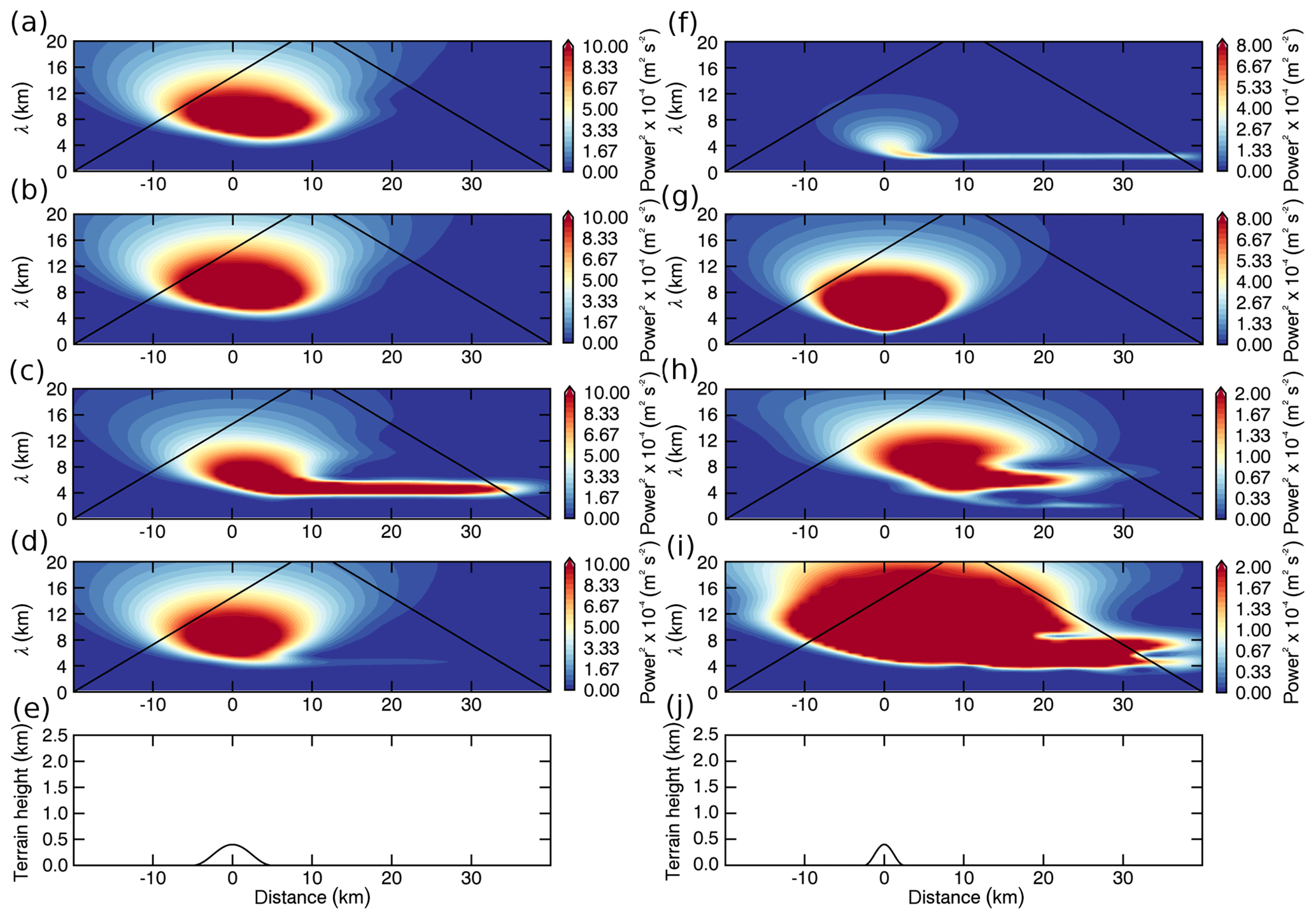
Figure 12Wavelet spectra of the vertical velocity of the idealized simulations shown in Fig. 11 in the vicinity of (a, c, f, h) and below (b, d, g, i) the top of the boundary layer or the inversion layer. Panels (e) and (j) show the idealized terrain. Panels (a, b) are for a neutral boundary layer without inversion and NU=0.01 s−1 (run 1), (c, d) are for a neutral boundary layer with an inversion of 3.3 K and NU=0.01 s−1 (run 2), (f, g) are for a neutral boundary layer with an inversion of 6.6 K and NU=0.02 s−1 (run 3), and (h, i) are for a stable troposphere (N=0.01 s−1) with a TIL of 6.6 K and NU=0.02 s−1 (run 4).
The second set of simulations (runs 5 and 6) uses a two-dimensional domain with 2016 and 1000 grid points in x and z directions, respectively, with grid increments of Δx=500 m and Δz=40 m. This results in a total domain size of about 1008 km × 40 km. The total integration time for these simulations is 16 h. This is longer than for the other set of simulations because it takes longer for the initial disturbance to reach the border of the larger domain. In contrast to the single-mountain simulations, these simulations, having more complex topography, do not reach quasi-steady state due to continuous interaction of waves from the different mountain peaks, reflected and trapped waves in the troposphere, and interfacial waves. Open boundaries are applied in the x direction. The model top is a rigid lid. The sponge layers at the horizontal edges of the domain are 40 km wide and the sponge layer at the top of the domain starts at 25 km altitude. The Scandinavian topography is interpolated on the 500 m grid from ASTER data. The initial profiles approximate the background conditions over southern Scandinavia given by the Stavanger radiosonde on 28 January 2016 (Fig. 14a–d). Simulations without and with a TIL are performed. The simplified initial horizontal velocity profile does not contain negative shear above the tropopause but negative shear establishes in the course of the simulation (dashed black profiles shown in Fig. 14a, c are located at −150 km distance 16 h after the start of the simulations).
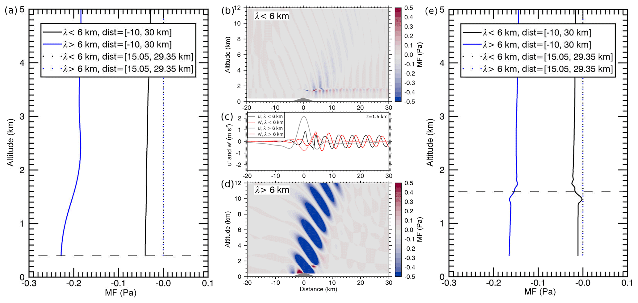
Figure 13Momentum flux (profiles) for (a) run 1 without boundary-layer inversion (Figs. 11a, 12a) and (b, d, e) run 2 with boundary-layer inversion (Figs. 11b, 12c) for two wave classes (horizontal wavelength smaller or larger 6 km). Profiles show averages for the full distance (solid) and for the downstream distance (dotted); horizontal dashed lines marks the top of the boundary layer. Panel (c) shows u′ and w′ for the two wave classes at 1.5 km altitude revealing their phase relationship right below the inversion, i.e. −90∘ for interfacial waves (black and red lines).
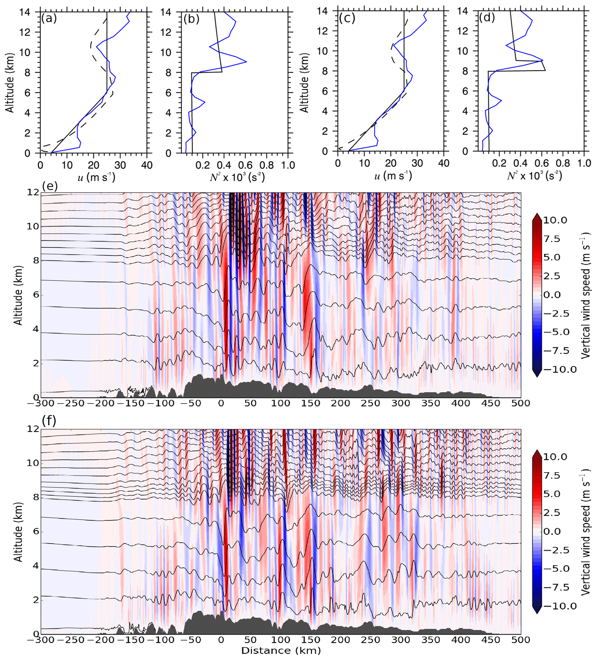
Figure 14Initial profiles (black solid) and vertical velocity for the simulations with more realistic terrain without TIL (a, b, e; run 5) and with TIL (c, d, f; run 6). The initial profiles approximate the background conditions over southern Scandinavia on 28 January 2016 (blue profiles show the Stavanger radiosonde data). Negative shear above the tropopause establishes in the course of the simulations (a, c; dashed black, time of 16 h, distance of −150 km).
Figures 14f and 15h (run 6) show that interfacial waves can also exist for the background conditions found on 28 January 2016 over southern Scandinavia. They are found downstream of the main mountain peak in the vicinity of the TIL (Figs. 14f and 15f) and their horizontal wavelength is approximately 8 km (Fig. 15h). The horizontal band pattern in the wavelet spectrum resembles the one of the idealized mountain simulations presented above (Fig. 12c, f, h). Small-scale interfacial waves are absent in the case of no TIL (Figs. 14e and 15a, c). They are only found in the TIL (Fig. 15f, h) but not below (Fig. 15g, i). Reflected waves with horizontal wavelengths between 10 and 30 km exist downstream of the main mountain peaks in the troposphere (Figs. 14e, f and 15d, i). It was already mentioned that the horizontal wavelength of the interfacial waves is independent of the generating terrain and determined by the background wind and stability. These two-dimensional simulations reveal the expected wavelength of the GWs over southern Scandinavia downstream of the main mountain ridge on 28 January 2016, i.e. approximately 8 km in the vicinity of the TIL and between 10 and 30 km in the troposphere. However, the interfacial waves in the simulation are not as dominant as in the measurements (Fig. 15h vs. RF07 FL2 and RF08 FL1 in Fig. 6b). There is a stronger signal of the upward-propagating MWs above the main mountain peaks (Fig. 15f, h).
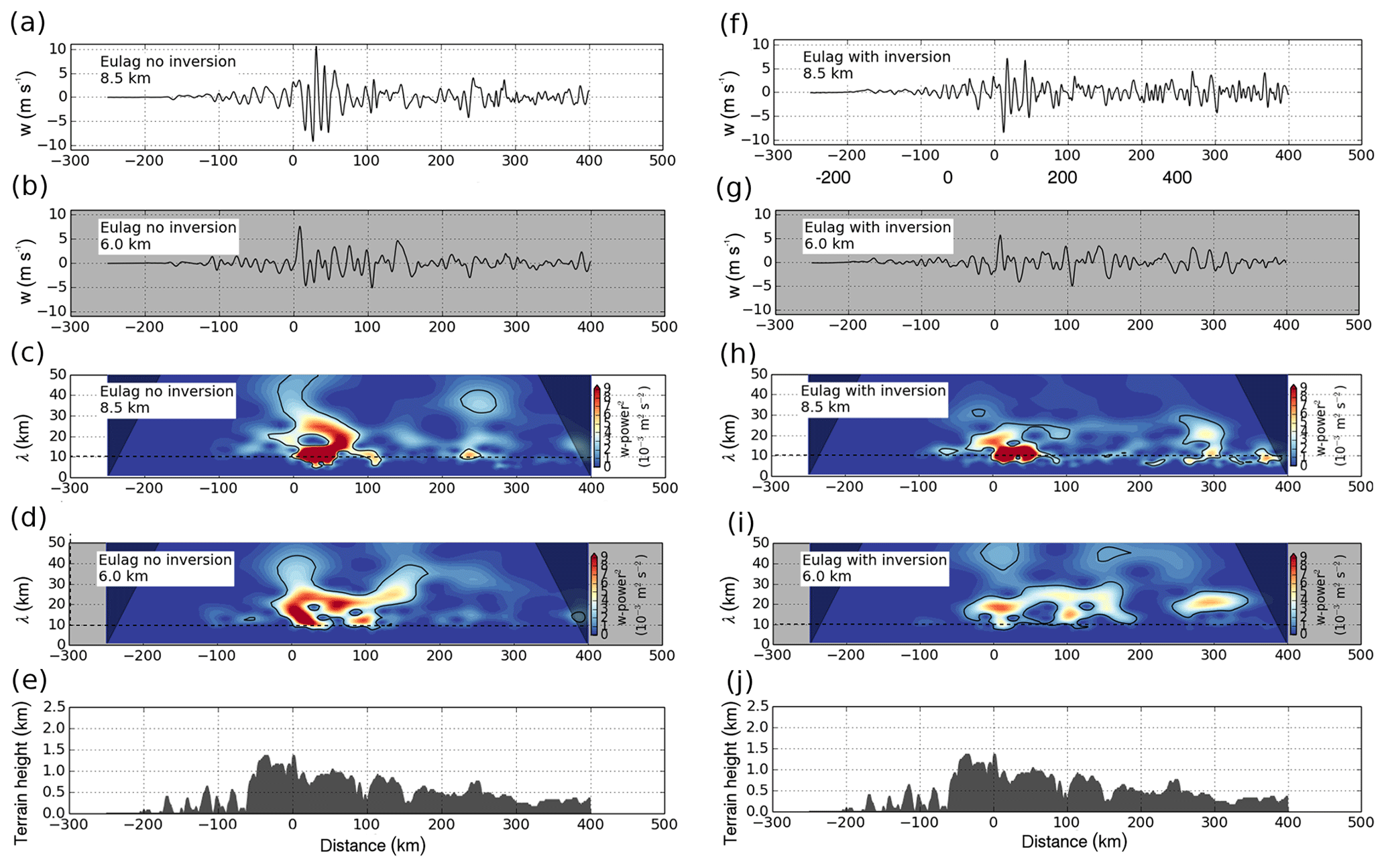
Figure 15Vertical velocity and corresponding wavelet spectra of the simulations shown in Fig. 14 (a–e without TIL, run 5, f–j with TIL, run 6). Panels (a, c, f, h) are at the altitude of the tropopause and (b, d, g, i) are below the tropopause. Panels (e) and (j) show the terrain in the domain.

Figure 16Averaged momentum fluxes for (a) run 5 (no TIL) and (b) run 6 (TIL) as mean for varying leg length (solid) with standard deviation (shading) and for the full leg distance [−300, 400 km] (dashed). Three wave classes are colour coded and the bold black line separates positive and negative fluxes.
MF profiles for the three wave classes (long (> 30 km), intermediate (10 to 30 km) and short (< 10 km)) are computed in the same way as for the measurements (Sect. 2.2.2) and are presented in Fig. 16. The MF profiles of the three wave classes clearly distinguish from each other. The fact that the mean MF profile computed from the set of sub-legs is close to the MF profile averaged for the full leg distance, which has the largest likelihood to capture the full wave cycles of the wave packages, supports that the sub-legs are chosen in a proper way. The pronounced kink in the MF profiles of the long and the short waves in the altitude range of 7 to 9 km is a clear feature of the effect of the TIL (Fig. 16b) and not visible in the no-TIL simulation (Fig. 16a). The amplitudes of the long waves (i.e. MWs) and the intermediate waves (i.e. reflected and trapped waves in the troposphere) and their resulting MF are overestimated compared to the observations (Figs. 6 and 15f–i). The MF is overall negative for these simulations but close to zero for the short waves. These findings are most likely an effect of the two-dimensional model setup. Interestingly, the MF of the long waves shows a larger magnitude in the simulation without TIL (Fig. 16a) compared to the simulation with TIL (Fig. 16b). The MF of the intermediate waves shows an opposite behaviour, i.e. smaller in magnitude in the simulation without TIL. This change in MF between the two simulations suggests stronger reflection of the MWs at the TIL. This is a finding that is in agreement with findings from the single-mountain simulations.
The atmospheric conditions during the MW case were characterized by moderate low level flow (∼ 10 m s−1), comparatively weak wind speed (∼ 30 m s−1) around the TIL and increasing wind speed above (Sec. 3.1.1). The coordinated airborne measurements including the downward-pointing DWL measurements revealed that the vertical velocity field was dominated by small horizontal scales with a decrease from around 20 to < 10 km in the vicinity of the TIL. These small scales were also found in the water vapour data and backscatter data of the DIAL (Sect. 3.1.2). The corresponding MF indicates wave reflection and trapping at the TIL (Figs. 7 and 10). It is known that atmospheric inversions can be wave guides leading to wave trapping and downstream wave propagation (Vosper, 2004; Sachsperger et al., 2015; Chouza et al., 2015; Fritts et al., 2018) but observations of downstream wave propagation of small-scale waves at tropopause inversions are rare (Smith et al., 2008; Woods and Smith, 2010).
In the course of investigating MW propagation in the UTLS with horizontal- and altitude-resolved airborne observations (Sect. 3.1.2), we found that the measured and simulated MF profile of the short waves (< 10 km) does not match the typical profile of Kelvin–Helmholtz instability that is characterized by one peak of positive MF (Mahalov et al., 2011). The shear was not strong enough to generate Kelvin–Helmholtz instabilities (Figs. 9a and 14a). Instead, the MF profile of the short waves varies around zero (Fig. 10). Trapped waves in the troposphere are known to have leg-averaged MFs of around zero (Woods and Smith, 2010; Georgelin and Lott, 2001). Our analyses revealed that the same is true for interfacial waves propagating horizontally along inversions. The MF profile of the long waves (> 30 km) is characterized by negative fluxes below and positive fluxes in the TIL which show similar magnitudes (Fig. 10). This is most likely due to partial reflection of these waves at the TIL. In the lower stratosphere, the leg-averaged MF was found to be positive (around 0.05 Pa). This is in contrast to the findings during DEEPWAVE where no positive leg-averaged MF was found in the lower stratosphere above New Zealand (Fig. 5b in Smith et al., 2016). However, analyses in Smith et al. (2016) are limited to waves having scales < 150 km and at least in ground-based lidar data downward-propagating waves were frequently observed in wintertime in the stratosphere above New Zealand (Kaifler et al., 2017). Local values of MF cospectra reach up to 0.034 kN m−1 in magnitude which is slightly below or half as large as the values found for an MW event during DEEPWAVE which were between 0.05 and 0.07 kN m−1 in magnitude (Portele et al., 2018).
The observed horizontal wavelengths in the vicinity of the TIL were clearly evanescent in the stratosphere (Fig. 5d). This excludes their direct propagation from above followed by their trapping in the TIL similar to Woods and Smith (2011). The presence of interfacial waves that are trapped on inversions and that are likely generated by MWs coming across the inversions (Sachsperger et al., 2017) has not yet been observed at TILs. Linear theory is able to describe the horizontal wavelength and the propagation of the interfacial waves (Vosper, 2004; Sachsperger et al., 2015, 2017). However, the amplitudes depend on the energy source, which is better described by hydraulic theory than by traditional linear models (Sachsperger et al., 2017). The traditional linear models link the energy source to the topography which is inaccurate for interfacial waves (especially for large amplitudes) because of nonlinear effects. Sachsperger et al. (2017) included the nonlinear effects in their model for the amplitudes of interfacial waves on the boundary-layer inversion by assuming that the interfacial waves originate at the density interface further aloft in the interior of the fluid and the energy source for these non-hydrostatic lee wave train is the energy convergence at an internal jump between two fluid layers of different densities.
The determined wave properties (observations) match those of interfacial waves (simulations) for which stability and wind conditions above the inversion determine the horizontal scales of the waves (Vosper, 2004; Sachsperger et al., 2015). The performed simulations show that the presence of the TIL is crucial in producing the trapped waves at tropopause altitude and vertical wind shear by the main MW was not sufficient in this case (Fig. 14a). However, the amplitudes of the interfacial waves were underestimated compared to the long and intermediate waves in the simulations. This can have several reasons. The amplitudes of interfacial waves depend on the amount of energy provided by the main wave source at the interface and the acting nonlinear processes (Sachsperger et al., 2017). It was not yet investigated how the interaction and generation processes depend on the model resolution and if the amplitudes increase with increasing resolution. The simulations were only two-dimensional, so they cannot capture effects of the fully three-dimensional mountain range. Moreover, potential additional energy input by downward-propagating larger-scale waves from stratospheric sources (e.g. polar night jet; Dörnbrack et al., 2018) or reflection of MWs in the middle and upper stratosphere are not included in the simulations. The positive leg-averaged MF for the long waves computed from HALO in situ data at an altitude of 13.3 km could be a hint of such additional energy input. In addition, also Krisch et al. (2020) found for the same HALO flight a checkerboard pattern in their three-dimensional temperature observations which allow to study large-scale waves (𝒪(100 km)) below the aircraft in the upper troposphere. This pattern suggests a possible level of reflection above flight altitude. The evaluation of these effects and the assessment of their sensitivities requires additional extensive model simulations which are beyond the scope of this paper and can be addressed in a future study.
The unique combination of observations from coordinated airborne in situ and lidar measurements and idealized large-eddy simulations revealed the occurrence of interfacial waves on the tropopause inversion during an MW event over southern Scandinavia on 28 January 2016. Such interfacial waves have already been observed on boundary-layer inversions but their concept has not been applied to tropopause inversions so far.
Strong shear induced by the main MW can cause Kelvin–Helmholtz instabilities which results in similar patterns in the vertical velocity field (Mahalov et al., 2011). Although the horizontal scales are close to 10 km, which is similar to T-REX observations (Smith et al., 2008; Woods and Smith, 2010), neither Kelvin–Helmholtz instability nor downward propagation of small-scale secondary GWs generated by MW breaking in the middle stratosphere can explain our observations. The vertical shear was not as pronounced as during the T-REX case (Mahalov et al., 2011) because the tropopause jet was not well established over southern Scandinavia on 28 January 2016. The wind speed influenced by the large-scale MW was only between 10 and 40 m s−1. The stratospheric critical horizontal wavelengths calculated from co-located radiosonde measurements are larger than the observed scales in the UTLS region which would hinder their direct downward propagation from a breaking region located higher up.
Our idealized simulations reveal that interfacial waves can occur also on tropopause inversions similar to boundary-layer inversions. Our analyses of the horizontal- and altitude-resolved airborne observations confirm that they actually do occur. As predicted by linear theory, the horizontal scale of those waves is determined by the wind and stability conditions above the inversion. They are found downstream of the main mountain peaks and their MF profile varies around zero. That is similar to tropospheric trapped waves and clearly distinguishes them from the MF profile of Kelvin–Helmholtz instability.
HALO and Falcon data are available on the HALO database (http://weather.uwyo.edu/upperair/sounding.html, station number 1415, last access August 2020, DLR, 2016). ECMWF data are available in the MARS archive (https://apps.ecmwf.int/archive-catalogue/, last access: August 2020, ECMWF, 2016). EULAG simulation data are available on the
ftp-server (ftp://ftp.pa.op.dlr.de/pub/gisinger/ACP_EULAG_2020/, last access: August 2020, Gisinger, 2020).
SG performed the large-eddy simulations and prepared the manuscript with contributions from all co-authors. JW did the analyses of the meteorological conditions and the aircraft in situ data. BW did the analyses of the wind lidar data.
The authors declare that they have no conflict of interest.
This article is part of the special issue “Sources, propagation, dissipation and impact of gravity waves (ACP/AMT inter-journal SI)”. It is not associated with a conference.
We thank the PIs and all participants of the GW-LCYCLE II campaign, in particular Markus Rapp and Andreas Dörnbrack for input and discussions. We thank Stephan Rahm and Martin Wirth for providing the lidar data, Andreas Giez and DLR FX for providing the in situ data, and Martina Bramberger and Tanja Portele for sharing their code and knowledge for the in situ data analyses. Access to the ECMWF data was possible through the special project “HALO Mission Support System”. Computational resources for EULAG simulations were provided by DKRZ. Radiosonde data were downloaded form the public archive of the University of Wyoming.
This research was funded by the German research initiative “Role of the Middle Atmosphere in
Climate (ROMIC/01LG1206A)” funded by the German Ministry of Research and Education in the project
“Investigation of the life cycle of gravity waves (GW-LCYCLE)” and by the Deutsche Forschungsgemeinschaft
(DFG) via the project MS-GWaves (GW TP/DO 1020/9 1).
The article processing charges for this open-access publication were covered by a Research Centre of the Helmholtz Association.
This paper was edited by Franz-Josef Lübken and reviewed by two anonymous referees.
Baines, P. G.: Topographic effects in stratified flows, Cambridge University Press, 1st edn., 1995. a
Birner, T.: Fine-scale structure of the extratropical tropopause region, J. Geophys. Res.-Atmos., 111, D04104, https://doi.org/10.1029/2005JD006301, 2006. a
Bramberger, M., Dörnbrack, A., Wilms, H., Gemsa, S., Raynor, K., and Sharman, R.: Vertically Propagating Mountain Waves – nA Hazard for High-Flying Aircraft?, J. Appl. Meteorol. Climatol., 57, 1957–1975, https://doi.org/10.1175/JAMC-D-17-0340.1, 2018. a
Brown, P. R. A.: Aircraft measurements of mountain waves and their associated momentum flux over the British Isles, Q. J. Roy. Meteor. Soc., 109, 849–865, https://doi.org/10.1002/qj.49710946211, 1983. a
Bögel, W. and Baumann, R.: Test and Calibration of the DLR Falcon Wind Measuring System by Maneuvers, J. Atmos. Ocean. Tech., 8, 5–18, https://doi.org/10.1175/1520-0426(1991)008<0005:TACOTD>2.0.CO;2, 1991. a
Chouza, F., Reitebuch, O., Groß, S., Rahm, S., Freudenthaler, V., Toledano, C., and Weinzierl, B.: Retrieval of aerosol backscatter and extinction from airborne coherent Doppler wind lidar measurements, Atmos. Meas. Tech., 8, 2909–2926, https://doi.org/10.5194/amt-8-2909-2015, 2015. a, b, c
Chouza, F., Witschas, B., and Reitebuch, O.: Heterodyne high-spectral-resolution lidar, Appl. Opt., 56, 8121–8134, 2017. a
Cruette, D.: Experimental study of mountain lee”waves by means of satellite photographs and aircraft measurements, Tellus, 28, 499–523, https://doi.org/10.3402/tellusa.v28i6.11318, 1976. a
DLR: HALO and Falcon data, available at: https://halo-db.pa.op.dlr.de/mission/3 (last access: August 2020), 2016. a
Dörnbrack, A., Gisinger, S., Kaifler, N., Portele, T. C., Bramberger, M., Rapp, M., Gerding, M., Söder, J., Žagar, N., and Jelić, D.: Gravity waves excited during a minor sudden stratospheric warming, Atmos. Chem. Phys., 18, 12915–12931, https://doi.org/10.5194/acp-18-12915-2018, 2018. a
Dunkerton, T.: On the Mean Meridional Mass Motions of the Stratosphere and Mesosphere, J. Atmos. Sci., 35, 2325–2333, https://doi.org/10.1175/1520-0469(1978)035<2325:OTMMMM>2.0.CO;2, 1978. a
Eckermann, S. D., Ma, J., and Broutman, D.: Effects of Horizontal Geometrical Spreading on the Parameterization of Orographic Gravity Wave Drag. Part I: Numerical Transform Solutions, J. Atmos. Sci., 72, 2330–2347, https://doi.org/10.1175/JAS-D-14-0147.1, 2015. a
ECMWF: ECMWF data, available at: https://apps.ecmwf.int/archive-catalogue/ (last access: August 2020), 2016. a
Fritts, D. C. and Alexander, J. M.: Gravity wave dynamics and effects in the middle atmosphere, Rev. Geophys., 41, 1003, https://doi.org/10.1029/2001RG000106, 2003. a
Fritts, D. C., Smith, R. B., Taylor, M. J., Doyle, J. D., Eckermann, S. D., Dörnbrack, A., Rapp, M., Williams, B. P., Pautet, P.-D., Bossert, K., Criddle, N. R., Reynolds, C. A., Reinecke, P. A., Uddstrom, M., Revell, M. J., Turner, R., Kaifler, B., Wagner, J. S., Mixa, T., Kruse, C. G., Nugent, A. D., Watson, C. D., Gisinger, S., Smith, S. M., Lieberman, R. S., Laughman, B., Moore, J. J., Brown, W. O., Haggerty, J. A., Rockwell, A., Stossmeister, G. J., Williams, S. F., Hernandez, G., Murphy, D. J., Klekociuk, A. R., Reid, I. M. and Ma, J.: The Deep Propagating Gravity Wave Experiment (DEEPWAVE): An airborne and ground-based exploration of gravity wave propagation and effects from their sources throughout the lower and middle atmosphere, B. Am. Meteorol. Soc., 97, 425–453, https://doi.org/10.1175/BAMS-D-14-00269.1, 2016. a, b
Fritts, D. C., Laughman, B., Wang, L., Lund, T. S., and Collins, R. L.: Gravity Wave Dynamics in a Mesospheric Inversion Layer: 1. Reflection, Trapping, and Instability Dynamics, J. Geophys. Res.-Atmos., 123, 626–648, https://doi.org/10.1002/2017JD027440, 2018. a, b
Georgelin, M. and Lott, F.: On the transfer of momentum by trapped lee waves: Case of the IOP 3 of PYREX, J. Atmos. Sci., 58, 3563–3580, https://doi.org/10.1175/1520-0469(2001)058<3563:OTTOMB>2.0.CO;2, 2001. a, b
Gisinger, S.: EULAG data, available at: ftp://ftp.pa.op.dlr.de/pub/gisinger/ACP_EULAG_2020/, last access: August 2020. a
Giez, A., Mallaun, C., Zöger, M., Dörnbrack, A., and Schumann, U.: Static Pressure from Aircraft Trailing-Cone Measurements and Numerical Weather-Prediction Analysis, J. Aircraft, 54, 1728–1737, https://doi.org/10.2514/1.C034084, 2017 a
Gill, A. E.: Atmosphere-Ocean Dynamics, International Geophysics Series, Volume 30, 1st edn., Academic Press, 1982. a
Grubišić, V. and Smolarkiewicz, P. K.: The Effect of Critical Levels on 3D Orographic Flows: Linear Regime, J. Atmos. Sci., 54, 1943–1960, https://doi.org/10.1175/1520-0469(1997)054<1943:TEOCLO>2.0.CO;2, 1997. a
Grubišić, V., Doyle, J. D., Kuettner, J., Dirks, R., Cohn, S. A., Pan, L. L., Mobbs, S., Smith, R. B., Whiteman, C. D., Czyzyk, S., Vosper, S., Weissmann, M., Haimov, S., Wekker, S. F. J. D., and Chow, F. K.: The Terrain-Induced Rotor Experiment, B. Am. Meteorol. Soc., 89, 1513–1533, https://doi.org/10.1175/2008BAMS2487.1, 2008. a
Heller, R., Voigt, C., Beaton, S., Dörnbrack, A., Giez, A., Kaufmann, S., Mallaun, C., Schlager, H., Wagner, J., Young, K., and Rapp, M.: Mountain waves modulate the water vapor distribution in the UTLS, Atmos. Chem. Phys., 17, 14853–14869, https://doi.org/10.5194/acp-17-14853-2017, 2017. a
Kaifler, N., Kaifler, B., Ehard, B., Gisinger, S., Dörnbrack, A., Rapp, M., Kivi, R., Kozlovsky, A., Lester, M., and Liley, B.: Observational indications of downward-propagating gravity waves in middle atmosphere lidar data, J. Atmos. Sol.-Terr. Phys., 162, 16–27, https://doi.org/10.1016/j.jastp.2017.03.003, 2017. a, b
Keller, T. L.: Implications of the hydrostatic assumption on atmospheric gravity waves, J. Atmos. Sci., 51, 1915–1929, https://doi.org/10.1175/1520-0469(1994)051<1915:IOTHAO>2.0.CO;2, 1994. a, b
Krisch, I., Preusse, P., Ungermann, J., Dörnbrack, A., Eckermann, S. D., Ern, M., Friedl-Vallon, F., Kaufmann, M., Oelhaf, H., Rapp, M., Strube, C., and Riese, M.: First tomographic observations of gravity waves by the infrared limb imager GLORIA, Atmos. Chem. Phys., 17, 14937–14953, https://doi.org/10.5194/acp-17-14937-2017, 2017. a
Krisch, I., Ern, M., Hoffmann, L., Preusse, P., Strube, C., Ungermann, J., Woiwode, W., and Riese, M.: Superposition of gravity waves with different propagation characteristics observed by airborne and space-borne infrared sounders, Atmos. Chem. Phys. Discuss., https://doi.org/10.5194/acp-2020-327, in review, 2020. a
Lane, T. P., Reeder, M. J., Morton, B. R., and Clark, T. L.: Observations and numerical modelling of mountain waves over the Southern Alps of New Zealand, Q. J. Roy. Meteor. Soc., 126, 2765–2788, https://doi.org/10.1002/qj.49712656909, 2000. a
Lane, T. P., Reeder, M. J., and Guest, F. M.: Convectively generated gravity waves observed from radiosonde data taken during MCTEX, Q. J. Roy. Meteor. Soc., 129, 1731–1740, https://doi.org/10.1256/qj.02.196, 2003. a
Lindzen, R. S.: Turbulence and Stress owing to Gravity-Wave and Tidal Breakdown, J. Geophys. Res.-Atmos., 86, 9707–9714, https://doi.org/10.1029/JC086iC10p09707, 1981. a
Lux, O., Lemmerz, C., Weiler, F., Marksteiner, U., Witschas, B., Rahm, S., Schäfler, A., and Reitebuch, O.: Airborne wind lidar observations over the North Atlantic in 2016 for the pre-launch validation of the satellite mission Aeolus, Atmos. Meas. Tech., 11, 3297–3322, https://doi.org/10.5194/amt-11-3297-2018, 2018. a
Mahalov, A., Moustaoui, M., and Grubišić, V.: A numerical study of mountain waves in the upper troposphere and lower stratosphere, Atmos. Chem. Phys., 11, 5123–5139, https://doi.org/10.5194/acp-11-5123-2011, 2011. a, b, c, d, e
Mallaun, C., Giez, A., and Baumann, R.: Calibration of 3-D wind measurements on a single-engine research aircraft, Atmos. Meas. Tech., 8, 3177–3196, https://doi.org/10.5194/amt-8-3177-2015, 2015. a
Marksteiner, U., Lemmerz, C., Lux, O., Rahm, S., Schäfler, A., Witschas, B., and Reitebuch, O.: Calibrations and wind observations of an airborne direct-detection wind LiDAR supporting ESA’s Aeolus mission, Remote Sens., 10, 2056, https://doi.org/10.3390/rs10122056, 2018. a
Oelhaf, H., Sinnhuber, B.-M., Woiwode, W., Bönisch, H., Bozem, H., Engel, A., Fix, A., Friedl-Vallon, F., Grooß, J.-U., Hoor, P., Johansson, S., Jurkat-Witschas, T., Kaufmann, S., Krämer, M., Krause, J., Kretschmer, E., Lörks, D., Marsing, A., Orphal, J., Pfeilsticker, K., Pitts, M., Poole, L., Preusse, P., Rapp, M., Riese, M., Rolf, C., Ungermann, J., Voigt, C., Volk, C. M., Wirth, M., Zahn, A., and Ziereis, H.: POLSTRACC: Airborne Experiment for Studying the Polar Stratosphere in a Changing Climate with the High Altitude and Long Range Research Aircraft (HALO), B. Am. Meteorol. Soc., 100, 2634–2664, https://doi.org/10.1175/BAMS-D-18-0181.1, 2019. a
Plougonven, R. and Zhang, F.: Internal gravity waves from atmospheric jets and fronts, Rev. Geophys., 52, 33–76, https://doi.org/10.1002/2012RG000419, 2014. a
Podglajen, A., Hertzog, A., Plougonven, R., and Legras, B.: Lagrangian temperature and vertical velocity fluctuations due to gravity waves in the lower stratosphere, Geophys. Res. Lett., 43, 3543–3553, https://doi.org/10.1002/2016GL068148, 2016. a
Portele, T. C., Dörnbrack, A., Wagner, J. S., Gisinger, S., Ehard, B., Pautet, P.-D., and Rapp, M.: Mountain-Wave Propagation under Transient Tropospheric Forcing: A DEEPWAVE Case Study, Mon. Weather Rev., 146, 1861–1888, https://doi.org/10.1175/MWR-D-17-0080.1, 2018. a, b, c
Prusa, J. M., Smolarkiewicz, P. K., and Garcia, R. R.: Propagation and Breaking at High Altitudes of Gravity Waves Excited by Tropospheric Forcing, J. Atmos. Sci., 53, 2186–2216, https://doi.org/10.1175/1520-0469(1996)053<2186:PABAHA>2.0.CO;2, 1996. a
Prusa, J. M., Smolarkiewicz, P. K., and Wyszogrodzki, A. A.: EULAG, a computational model for multiscale flows, Comput. Fluids, 37, 1193–1207, https://doi.org/10.1016/j.compfluid.2007.12.001, 2008. a, b
Queney, P.: The problem of air flow over mountains: a summary of theoretical studies, B. Am. Meteorol. Soc., 29, 16–26, 1948. a, b
Ralph, F. M., Neiman, P. J., Keller, T. L., Levinson, D., and Fedor, L.: Observations, simulations, and analysis of nonstationary trapped lee waves, J. Atmos. Sci., 54, 1308–1333, https://doi.org/10.1175/1520-0469(1997)054<1308:OSAAON>2.0.CO;2, 1997. a
Sachsperger, J., Serafin, S., and Grubišić, V.: Lee Waves on the Boundary-Layer Inversion and Their Dependence on Free-Atmospheric Stability, Front. Earth Sci., 3, 70, https://doi.org/10.3389/feart.2015.00070, 2015. a, b, c, d, e, f, g
Sachsperger, J., Serafin, S., Grubišić, V., Stiperski, I., and Paci, A.: The amplitude of lee waves on the boundary‐layer inversion, Q. J. Roy. Meteor. Soc., 143, 27–36, https://doi.org/10.1002/qj.2915, 2017. a, b, c, d, e, f, g
Sato, K., Watanabe, S., Kawatani, Y., Tomikawa, Y., Miyazaki, K., and Takahashi, M.: On the origins of mesospheric gravity waves, Geophys. Res. Lett., 36, L19801, https://doi.org/10.1029/2009GL039908, 2009. a
Schäfler, A., Craig, G., Wernli, H., Arbogast, P., Doyle, J. D., McTaggart-Cowan, R., Methven, J., Rivière, G., Ament, F., Boettcher, M., Bramberger, M., Cazenave, Q., Cotton, R., Crewell, S., Delanoë, J., Dörnbrack, A., Ehrlich, A., Ewald, F., Fix, A., Grams, C. M., Gray, S. L., Grob, H., Groß, S., Hagen, M., Harvey, B., Hirsch, L., Jacob, M., Kölling, T., Konow, H., Lemmerz, C., Lux, O., Magnusson, L., Mayer, B., Mech, M., Moore, R., Pelon, J., Quinting, J., Rahm, S., Rapp, M., Rautenhaus, M., Reitebuch, O., Reynolds, C. A., Sodemann, H., Spengler, T., Vaughan, G., Wendisch, M., Wirth, M., Witschas, B., Wolf, K., and Zinner, Tobias: The North Atlantic waveguide and downstream impact experiment, B. Am. Meteorol. Soc., 99, 1607–1637, 2018. a
Schmugge, T. J., Abrams, M. J., Kahle, A. B., Yamaguchi, Y., and Fujisada, H.: Advanced Spaceborne Thermal Emission and Reflection Radiometer (ASTER), Proc. SPIE Remote Sensing for Agriculture, Ecosystems, and Hydrology IV, 4879, https://doi.org/10.1117/12.469693, 2003. a
Scorer, R.: Theory of waves in the lee of mountains, Q. J. Roy. Meteorol. Soc., 75, 41–56, 1949. a, b
Shibuya, R., Sato, K., Tsutsumi, M., Sato, T., Tomikawa, Y., Nishimura, K., and Kohma, M.: Quasi-12 h inertia–gravity waves in the lower mesosphere observed by the PANSY radar at Syowa Station (39.6° E, 69.0° S), Atmos. Chem. Phys., 17, 6455–6476, https://doi.org/10.5194/acp-17-6455-2017, 2017. a
Smith, R. B.: The influence of mountains on the atmosphere, Adv. Geophys., 21, 87–230, https://doi.org/10.1016/S0065-2687(08)60262-9, 1979. a
Smith, R. B. and Kruse, C. G.: Broad-Spectrum Mountain Waves, J. Atmos. Sci., 74, 1381–1402, https://doi.org/10.1175/JAS-D-16-0297.1, 2017. a
Smith, R. B., Woods, B. K., Jensen, J., Cooper, W. A., Doyle, J. D., Jiang, Q., and Grubišić, V.: Mountain Waves Entering the Stratosphere, J. Atmos. Sci., 65, 2543–2562, https://doi.org/10.1175/2007JAS2598.1, 2008. a, b, c, d
Smith, R. B., Nugent, A. D., Kruse, C. G., Fritt, D. C., Doyle, J. D., Eckermann, S. D., Taylor, M. J., Dörnbrack, A., Uddstrom, M., Cooper, W., Romashkin, P., Jensen, J., and Beaton, S.: Stratospheric gravity wave fluxes and scales during DEEPWAVE, J. Atmos. Sci., 73, 2851–2869, https://doi.org/10.1175/JAS-D-15-0324.1, 2016. a, b, c
Smolarkiewicz, P. K., Margolin, L. G., and Wyszogrodzki, A. A.: A Class of Nonhydrostatic Global Models, J. Atmos. Sci., 58, 349–364, https://doi.org/10.1175/1520-0469(2001)058<0349:ACONGM>2.0.CO;2, 2001. a, b
Sutherland, B. R.: Internal Gravity Waves 1st Edition, Cambridge University Press, 2010. a
Torrence, C. and Compo, G. P.: A practical guide to wavelet analysis, B. Am. Meteorol. Soc., 79, 61–78, https://doi.org/10.1175/1520-0477(1998)079<0061:APGTWA>2.0.CO;2, 1998. a
Vadas, S. L., Fritts, D. C., and Alexander, M. J.: Mechanism for the Generation of Secondary Waves in Wave Breaking Regions, J. Atmos. Sci., 60, 194–214, https://doi.org/10.1175/1520-0469(2003)060<0194:MFTGOS>2.0.CO;2, 2003. a
Vosper, S.: Inversion effects on mountain lee waves, Q. J. Roy. Meteor. Soc., 130, 1723–1748, https://doi.org/10.1256/qj.03.63, 2004. a, b, c, d, e, f, g, h, i
Wirth, M., Fix, A., Mahnke, P., Schwarzer, H., Schrandt, F., and Ehret, G.: The airborne multi-wavelength water vapor differential absorption lidar WALES: system design and performance, Appl. Phys. B, 96, 201–213, 2009. a
Witschas, B., Rahm, S., Dörnbrack, A., Wagner, J. S., and Rapp, M.: Airborne wind lidar measurements of vertical and horizontal winds for the investigation of orographically induced gravity waves, J. Atmos. Ocean. Tech., 34, 1371–1386, https://doi.org/10.1175/JTECH-D-17-0021.1, 2017. a, b
Witschas, B., Lemmerz, C., Geiß, A., Lux, O., Marksteiner, U., Rahm, S., Reitebuch, O., and Weiler, F.: First validation of Aeolus wind observations by airborne Doppler wind lidar measurements, Atmos. Meas. Tech., 13, 2381–2396, https://doi.org/10.5194/amt-13-2381-2020, 2020a. a
Witschas, B., Rahm, S., Wagner, J., and Gisinger, S.: Airborne measurements of gravity wave momentum flux by means of a coherent wind lidar, Atmos. Meas. Tech., in preparation, 2020b. a
Woods, B. K. and Smith, R. B.: Energy Flux and Wavelet Diagnostics of Secondary Mountain Waves, J. Atmos. Sci., 67, 3721–3738, https://doi.org/10.1175/2009JAS3285.1, 2010. a, b, c, d, e, f
Woods, B. K. and Smith, R. B.: Short-Wave Signatures of Stratospheric Mountain Wave Breaking, J. Atmos. Sci., 68, 635–656, https://doi.org/10.1175/2010JAS3634.1, 2011. a, b
Wright, C. J., Hindley, N. P., Hoffmann, L., Alexander, M. J., and Mitchell, N. J.: Exploring gravity wave characteristics in 3-D using a novel S-transform technique: AIRS/Aqua measurements over the Southern Andes and Drake Passage, Atmos. Chem. Phys., 17, 8553–8575, https://doi.org/10.5194/acp-17-8553-2017, 2017. a
Wurtele, M., Sharman, R., and Keller, T.: Analysis and simulations of a troposphere–stratosphere gravity wave model. Part I, J. Atmos. Sci., 44, 3269–3281, https://doi.org/10.1175/1520-0469(1987)044<3269:AASOAT>2.0.CO;2, 1987. a
Wurtele, M., Sharman, R., and Datta, A.: Atmospheric lee waves, Ann. Rev. Fluid Mech., 28, 429–476, https://doi.org/10.1146/annurev.fl.28.010196.002241, 1996. a
https://www.ecmwf.int/en/forecasts/documentation-and-support/changes-ecmwf-model/cy41r1-summary-changes, last access: October 2018
https://www.ecmwf.int/en/forecasts/documentation-and-support/137-model-levels, last access: October 2018
Wavelet software was provided by Christopher Torrence and Gilbert P. Compo, and is available at http://atoc.colorado.edu/research/wavelets/, last access November 2019
http://www2.mmm.ucar.edu/eulag/, last access: November 2019
Sounding data are from http://weather.uwyo.edu/upperair/sounding.html, station number 1415 (last access: August 2020).