Reactive nitrogen (NO_y) and ozone responses to energetic electron precipitation during Southern Hemisphere winter

Energetic particle precipitation (EPP) affects the chemistry of the polar middle atmosphere by producing reactive nitrogen (NO_y) and hydrogen (HO_x) species, which then catalytically destroy ozone. Recently, there have been major advances in constraining these particle impacts through a parametrization of NO_y based on high-quality observations. Here we investigate the effects of low (auroral) and middle (radiation belt) energy range electrons, separately and in combination, on reactive nitrogen and hydrogen species as well as on ozone during Southern Hemisphere winters from 2002 to 2010 using the SOCOL3-MPIOM chemistry-climate model. Our results show that, in the absence of solar proton events, low-energy electrons produce the majority of NO_y in the polar mesosphere and stratosphere. In the polar vortex, NO_y subsides and affects ozone at lower altitudes, down to 10 hPa. Comparing a year with high electron precipitation with a quiescent period, we found large ozone depletion in the mesosphere; as the anomaly propagates downward, 15 % less ozone is found in the stratosphere during winter, which is confirmed by satellite observations. Only with both low- and middle-energy electrons does our model reproduce the observed stratospheric ozone anomaly.

1 Introduction

Energetic particles originating from the Sun, the magnetosphere, or outside the solar system continuously precipitate into the Earth's atmosphere and can influence atmospheric processes. They ionize neutral air molecules, especially in the middle and upper polar atmosphere, and create odd nitrogen and hydrogen species, NO_x ($\left[\mathrm{N}\right]+\left[\mathrm{NO}\right]+\left[{\mathrm{NO}}_{\mathrm{2}}\right]$) and HO_x ([H] + [OH] + [HO₂]). NO_x and HO_x radicals can catalytically deplete ozone. The in situ destruction of ozone in the mesosphere is characteristic of HO_x due to its fast reaction rates (Bates and Nicolet, 1950). On the other hand, NO_x, in the absence of sunlight, subsides within the downwelling branch of the overturning circulation, affecting ozone concentrations at lower altitudes (Solomon et al., 1982).

High-energy particles, i.e. solar protons (Jackman et al., 2008) and radiation belt electrons (Arsenovic et al., 2016; Semeniuk et al., 2011), can penetrate directly into the mesosphere and stratosphere. Radiation belt electrons (energies > 30 keV) impact chemistry below 90 km in the atmosphere (Turunen et al., 2009). Electrons of lower energies (< 30 keV, auroral) originate from the magnetosphere as well as the radiation belt electrons (Mironova et al., 2015), but they get accelerated in the magnetotail and precipitate into the lower thermosphere in the auroral ovals (55–70^∘ geomagnetic latitude) (Baker et al., 2001; Barth et al., 2003). Their peak impact is above 90 km in the thermosphere (Turunen et al., 2009).

There have been numerous attempts to include low-energy electrons (LEE) in climate models. Chemistry-climate or chemistry-transport models with top in the thermosphere, e.g. HAMMONIA (Schmidt et al., 2006), KASIMA (Reddmann et al., 2010), and WACCM (Andersson et al., 2018; Marsh et al., 2007), have included effects of LEE directly because they deposit their energy within the model domain. For climate models that have an upper lid below the thermosphere, a prescription of LEE either as NO_y influx through the model top or as concentrations (number density) in the upper model boxes is recommended (Matthes et al., 2017). Baumgaertner et al. (2009) developed a parameterization of this flux based on the geomagnetic activity A_p index, a daily worldwide measure of the effects of solar wind on the Earth's magnetic field. When incorporated into a chemistry-climate model, results showed significant ozone depletion in the mesosphere and stratosphere (Baumgaertner et al., 2011). For the SOCOL chemistry-climate model, Rozanov et al. (2012) also found significant ozone decreases in the mesosphere and stratosphere, with peak values around 10 % in September around 36 km altitude over the Antarctic.

Funke et al. (2016) recently developed a semi-empirical model that calculates concentrations and fluxes of mesospheric and stratospheric NO_y compounds ($\left[\mathrm{NO}\right]+\left[{\mathrm{NO}}_{\mathrm{2}}\right]+\mathrm{2}\times \left[{\mathrm{N}}_{\mathrm{2}}{\mathrm{O}}_{\mathrm{5}}\right]+\left[{\mathrm{HNO}}_{\mathrm{3}}\right]+\left[{\mathrm{ClONO}}_{\mathrm{2}}\right]$) based on the Michelson Interferometer for Passive Atmospheric Sounding (MIPAS) observations. The model exploits the nearly linear relationship in the mesosphere between the A_p index with observed NO_y produced by EPP. This advance in the representation of LEE in climate models motivates us to investigate whether LEE can have a larger impact on atmospheric chemistry than previously thought (Rozanov et al., 2012). Moreover, this LEE parameterization is a part of the recommended solar forcing dataset for climate models within the upcoming Coupled Model Intercomparison Project Phase 6 (CMIP-6, Matthes et al., 2017).

It is crucial to have a realistic representation of EPP in models as the introduced signal impacts atmospheric chemistry and potentially regional climate (Baumgaertner et al., 2011; Maliniemi et al., 2014; Rozanov et al., 2012; Seppälä et al., 2013). Sinnhuber et al. (2018) showed the impact of one possible implementation of the new Funke et al. (2016) LEE NO_y parameterization in their EMAC model on NO_y and ozone; however, they did not explicitly consider MEE. Here we present results from our state-of-the-art chemistry-climate model, employing a different implementation of the same parameterization of LEE together with the previous representations of other energetic particles. This paper focuses on evaluating NO_x and ozone response to LEE and MEE precipitation, separately and in combination, in Antarctic winters (JJA: June, July, and August), in order to avoid the more complicated Arctic polar vortex with its high variability and strong dependence on meteorological conditions (Hitchcock et al., 2013). We compare our results with the satellite observations.

2 Methods

We used the SOCOL3-MPIOM coupled chemistry-climate model (Muthers et al., 2014; Stenke et al., 2013). The atmospheric dynamic component of the model is ECHAM5.4 (Roeckner and Bäuml, 2003), coupled to the MEZON air chemistry module (Egorova et al., 2003; Rozanov et al., 1999) and the MPIOM interactive ocean module (Jungclaus et al., 2006; Marsland et al., 2002). We carried out the experiments with T31 spectral resolution on 39 vertical levels from the surface up to 0.01 hPa (∼80 km).

The model boundary conditions and parameterizations are identical to those described in Arsenovic et al. (2016), except for the LEE parameterization. Following Calisto et al. (2011), galactic cosmic rays (GCR) are parameterized as a function of geomagnetic latitude, pressure, and solar modulation potential. Ionization by solar protons (SP) is treated according to Jackman et al. (2008) and ionization by middle-energy electrons (MEE) with energies between 30 and 300 keV is taken from the Atmospheric Ionization Module Osnabrück (AIMOS) v1.6 (Arsenovic et al., 2016; Wissing and Kallenrode, 2009). Electrons of energies higher than 300 keV are not included in the model due to a lack of adequate parameterization.

For LEE, we are using the semi-empirical model for NO_y influx by Funke et al. (2016) through the model top at 0.01 hPa (75–80 km in polar conditions). Although MIPAS scans the atmosphere up to 68 km altitude, the applicability of this parameterization above 70 km has been validated by comparison with MIPAS middle- and upper-atmosphere observations (scanning up to 100 and 170 km, respectively). As more than 99 % of the NO_y at this altitude is in the form of nitrogen monoxide (nitric oxide), NO (Brasseur and Solomon, 2005), we approximate the NO_y influx calculated by the semi-empirical model as NO influx at this level in SOCOL3-MPIOM. As mentioned before, LEE precipitate above 90 km and MEE precipitate between 70 and 90 km altitude (Turunen et al., 2009). However, because of our model top at 80 km, here we consider electrons that precipitate below 80 km to be MEE and electrons that precipitate above the model top to be LEE.

Matthes et al. (2017) and Sinnhuber et al. (2018) also implemented the parameterization by Funke et al. (2016) in the EMAC model. They used a different approach, prescribing NO concentrations (instead of fluxes through the model top) in the model within the 0.09–0.01 hPa layer and performed the simulations with specified dynamics. Prescribing concentrations requires overwriting NO simulated values. It is inconsistent with the treatment of the physical and chemical processes in our model leading to accumulation of NO_y. This is not the case for the influx approach and therefore we prescribe the NO influx instead of NO concentrations; however, prescribed NO concentrations can be used for models with different treatments of the chemical and transport processes.

Figure 1 shows the monthly mean geomagnetic A_p index that covers our simulated period. Period 2002–2005 was characterized by a rather high A_p index and the 2006–2010 period by low values. For our simulations, we have used daily NO fluxes calculated from daily A_p indices.

Four sets of six-member ensemble simulations were carried out, covering the 2002–2010 period: the “ALL” simulation, which includes all energetic particles (GCR, SP, MEE, and LEE), the “LEE” simulation (GCR, SP, and LEE), the “MEE” simulation (GCR, SP, and MEE), and the reference “REF” simulation (GCR and SP). All these simulations have the same model boundary conditions and differ only in the inclusion of the low-/middle-energy electron precipitation.

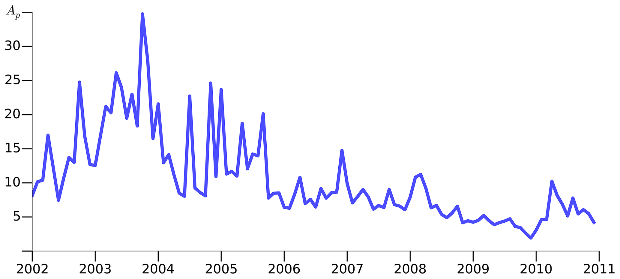
Figure 1 The monthly mean geomagnetic A_p index during the simulated period: years 2002–2005 were rather active, while the period 2006–2010 was geomagnetically quiescent (CMIP-6 dataset; Matthes et al., 2017).

We used two satellite datasets to evaluate our model results: MIPAS for nitrogen species and the Microwave Limb Sounder (MLS) for ozone. MIPAS was a Fourier transform spectrometer aboard the ENVISAT satellite (Fischer et al., 2008). The quality of MIPAS NO_y and individual NO_y species has been extensively assessed in SPARC (2017), as well as specific validation studies (e.g. Bender et al., 2015; Sheese et al., 2016). The top altitude of the MIPAS nominal limb scans is 68 km, but it also contains information on the NO_y above, though with low vertical resolution. Since it provides the entire NO_y budget in the upper atmosphere (with a vertical resolution of 3–5 km), we used this dataset to validate simulated NO_y.

The MLS aboard the Aura satellite (Waters et al., 2006) has provided daily measurements of ozone profiles (Froidevaux et al., 2008) in the middle and upper atmosphere since August 2004. We used MLS observations to evaluate modelled ozone. The vertical resolution of MLS O₃ (v4.2) is about 3 km in the stratosphere, increasing up to about 5 km in the mesosphere (Livesey et al., 2018).

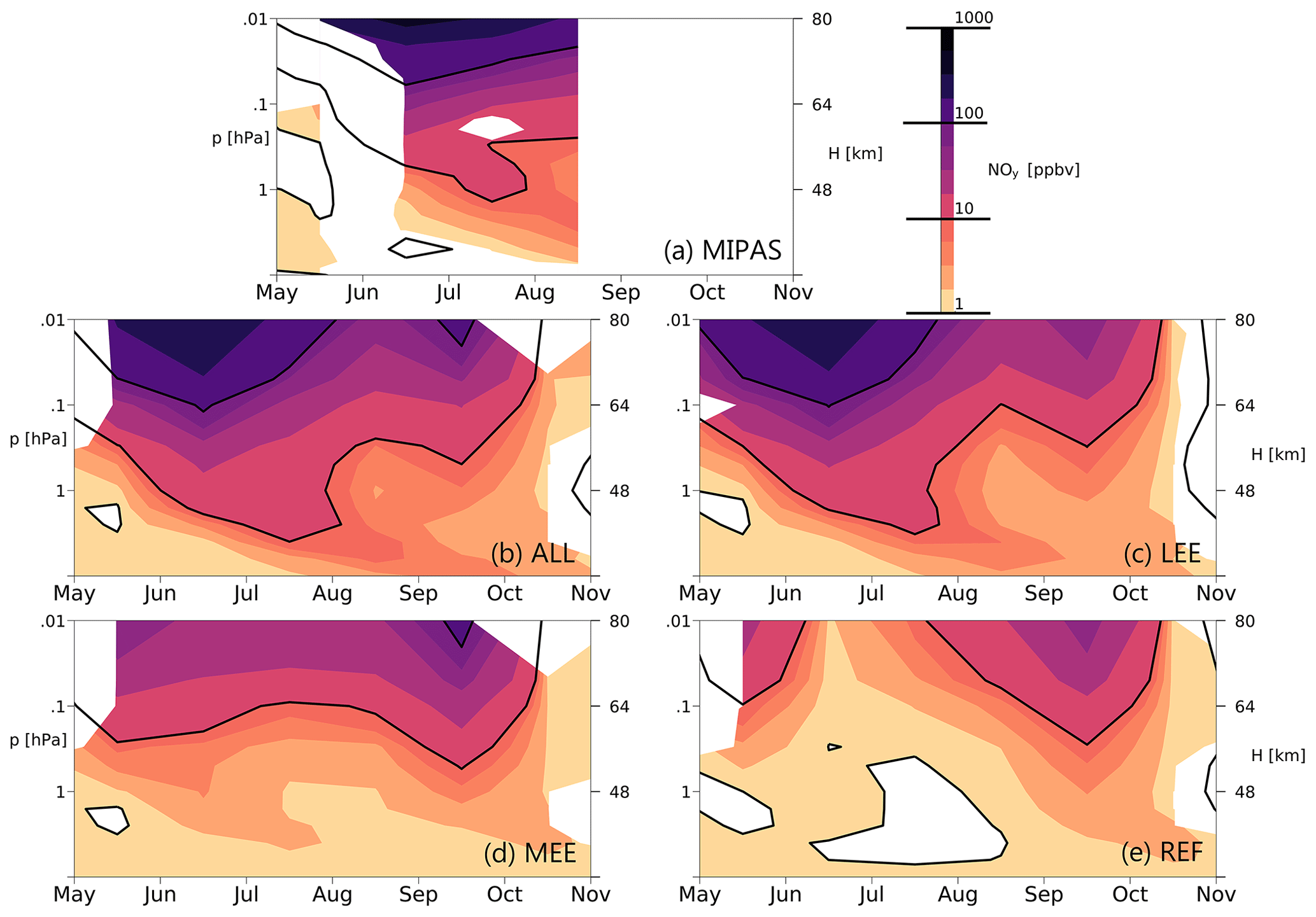
Figure 2 Monthly mean NO_y volume mixing ratio anomaly in ppbv for the Southern Hemisphere (> 70^∘ S average) calculated as the difference of the year 2005 and the average of 2006–2010. (a) MIPAS observations; (b) ensemble mean of ALL simulations; (c) ensemble mean of LEE simulations; (d) ensemble mean of MEE simulations; (e) ensemble mean of REF simulations. Colour levels are 1, 2.5, 5, 7.5, 10, 25, 50, 75, 100, 250, 500, 750, and 1000 ppbv and the black contour lines highlight 1, 10, 100, and 1000 ppbv. Coloured regions are significant at the 99 % confidence level (calculated using a Student's t test).

3 Results

3.1 NO_y enhancement propagation

Figure 2 shows the difference in NO_y concentration between the geomagnetically active year 2005 and the mean over the geomagnetically quiescent period 2006–2010 averaged over 70–90^∘ S. Even though year 2003 on average has higher Ap, here we choose year 2005 as the geomagnetically active year. This allows us to compare modelled NO_y and ozone using two different satellite datasets, MIPAS and MLS (which have been available only since 2005). MIPAS data are unavailable from September 2005 to the end of the year, but our main period of interest is JJA, which is well covered by the observations.

The MIPAS observations (Fig. 2a) show a NO_y enhancement throughout the mesosphere and upper stratosphere. In terms of mixing ratio, the highest increase of 500–600 ppbv is found in the upper mesosphere around 0.01 hPa (∼80 km). There, the highest monthly values are observed in June. In the following months, this anomaly descends and reaches lower levels. In July, the NO_y enhancement of around 10 ppbv reaches the upper stratosphere around 2 hPa, and the increase, although smaller, is visible all the way down to 10 hPa. In the following months, the MIPAS nominal data were unavailable due to special observation mode campaigns.

The ALL experiment (Fig. 2b) shows a very similar pattern of NO_y to the observations. The NO_y increase of 500–600 ppbv in the upper mesosphere around 0.01 hPa is similar to the MIPAS observations. However, the wintertime NO_y peak below is slightly overestimated in the model compared to MIPAS. This is particularly visible in the lower mesosphere in June, as the modelled 100 ppbv NO_y enhancement reaches 0.1 hPa. The mesospheric anomaly extends into the stratosphere, but remains confined to the upper stratosphere, above 10 hPa, as in observations. The modelled NO_y overestimation suggests that downward transport is somewhat too fast in the model, or that the photochemical lifetime of NO_y is too long, or that horizontal mixing with mid-latitudes is underestimated. The modelled NO_y enhancement in September stems from an SP event (NOAA). In contradiction to our results, the EMAC model slightly underestimates NO_y even during polar summer, for two pressure levels, 0.1 and 1 hPa (Matthes et al., 2017). Sinnhuber et al. (2018) showed underestimation of NO_y in the upper mesosphere in the EMAC and KASIMA models and overestimation of NO_y in the 3dCTM model in the Southern Hemisphere compared to MIPAS observations.

The LEE simulation (Fig. 2c) shows very similar anomalies to ALL. The largest differences are in the upper mesosphere, where LEE anomalies reach around 400 ppbv, which is underestimated compared to the 500–600 ppbv found in MIPAS and ALL. A second interesting difference compared to ALL is the SP event in September. In the LEE simulation, it reaches around 60 ppbv, while in ALL it exceeds 100 ppbv. This difference comes from increased MEE precipitation that coincided with the SP event (see Arsenovic et al., 2016, Fig. 1a). During strong SP events protons can contaminate the highest electron channel, so this channel is excluded from the AIMOS dataset (Yando et al., 2011). Although some degree of contamination is still possible in the lower channels, protons are not the sole cause of the increased NO_y in this SP event. That is, SP events are often associated with large coronal mass ejections that form a shock in front of them. Once the shock hits the Earth it often leads to a geomagnetic storm which leads to acceleration of electrons of > 30 keV energies. Therefore, increased MEE precipitation often happens very shortly after an SP event because the shock and the geomagnetic storm are related to the same coronal mass ejection driver (Asikainen and Ruopsa, 2016).

The MEE simulation (Fig. 2d) is drastically different from MIPAS as well as the ALL and LEE simulations. Although NO_y enhancement in the modelled geomagnetically active year exists, it is significantly decreased compared with the previous results. The modelled NO_y mesospheric anomaly peak is absent and enhancement of 10 ppbv does not reach the stratosphere. Nevertheless, although less intense, increased NO_y is present throughout the mesosphere and stratosphere, and the NO_y increase in September due to the SP event again exceeds 100 ppbv, as in the ALL simulation.

The reference run in Fig. 2e shows NO_y increase due to the SP events in the year 2005. In this year, there were six observed SP events in the shown time frame – 14 May, 16 June, 14 and 27 July, 22 August, and 8 September (NOAA). In the geomagnetically inactive period, 2006–2010, there were no observed SP events in the presented months. Therefore, by excluding electron precipitation, the SP events alone cannot reproduce the observed features.

From the presented months, we conclude that the inclusion of only LEE was sufficient to reproduce most of the NO_y enhancements. The MEE contribution to NO_y increases is minor and brings the model closer to observations mainly in the upper mesosphere. As coronal mass ejections drive SP events and they can have an impact on the precipitation from the outer Van Allen belt (Asikainen and Ruopsa, 2016; Pierrard and Lopez Rosson, 2016), MEE precipitation could significantly contribute to NO_y increases in such events.

3.2 O₃ anomaly propagation

In the study of Matthes et al. (2017), ozone responses were evaluated by comparing high and low geomagnetic activity years, and their estimate shows good agreement with satellite observations (Fytterer et al., 2015). To evaluate our simulated ozone responses, we follow a similar approach to that used in Matthes et al. (2017); that is, we compared our simulations with observations from MLS. We analysed the 2005–2010 period when both simulation and MLS data are available.

Ozone anomalies from MLS observations during the high geomagnetically active year are depicted in Fig. 3a. They are calculated as the difference averaged over 70–90^∘ S between the active year (2005) and the average of geomagnetically quiescent years (2006–2010) divided by the ozone averaged over the whole period (2005–2010). Observations show around 20 % less ozone in the upper mesosphere (< 0.1 hPa) occurring mostly in the JJA period. The exception is the SP event on 8 September 2005. It created an ozone anomaly of up to 80 % stretching throughout the whole mesosphere. The mesosphere below 0.1 hPa does not show a statistically significant difference between the geomagnetically active and quiescent years in the absence of SP events. The observed negative ozone anomaly appears again around the stratopause in late June and propagates downwards to nearly 10 hPa in early September. The peak ozone anomaly occurs in August around 3 hPa, reaching ∼15 %. Our results agree with the results from previous modelling studies (Reddmann et al., 2010; Rozanov et al., 2012; Sinnhuber et al., 2018) and observations (Damiani et al., 2016; Fytterer et al., 2015).

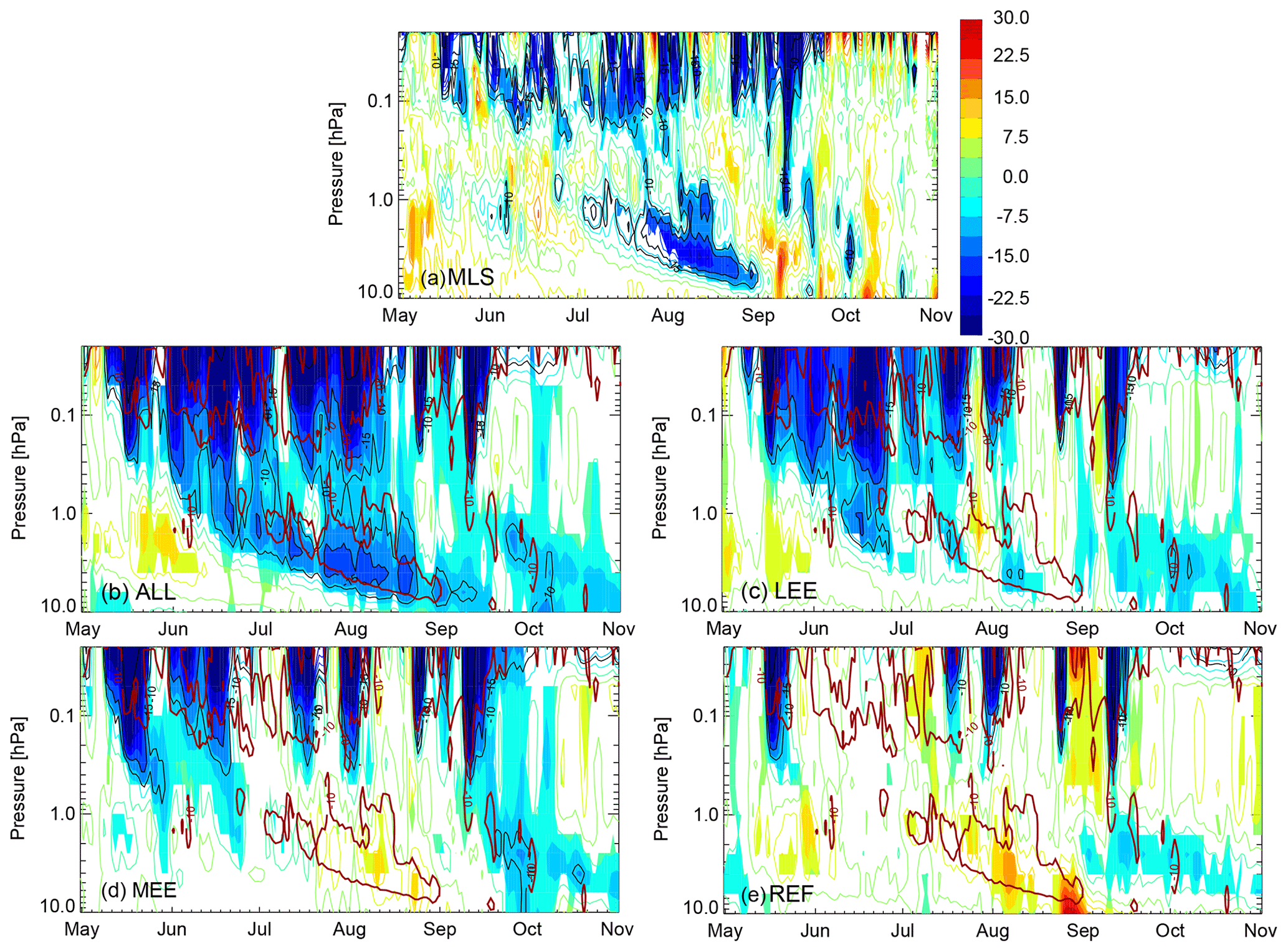
Figure 3 Monthly mean ozone anomaly poleward of 70^∘ S calculated as the difference of year 2005 and average of 2006–2010 relative to the 2005–2010 period. (a) MLS observations; (b) ensemble mean of ALL simulations; (c) ensemble mean of LEE simulations; (d) ensemble mean of MEE simulations; (e) ensemble mean of REF simulations. Black lines highlight −10 %, −15 %, and −50 % and dark red lines mark −10 % from MLS observations on every plot. Note that mesospheric ozone depletion reaches 80 %–90 % during some strong solar proton events. Coloured regions are significant at the 99 % confidence level (calculated using a Student's t test).

The ALL simulation (Fig. 3b) shows a negative ozone anomaly in the mesosphere as well. However, the magnitude is generally higher (around 30 %), and it is present from May to September. The September 2005 SP event is visible in the model simulations as well and descends from around 1 hPa in late September, reaching 10 hPa in late October. A similar pattern, but less obvious, is seen in the observations. Ozone anomalies in the lower mesosphere (0.5–0.1 hPa) are more pronounced in the model than in MLS observations. This is particularly evident in June when the modelled upper-mesosphere anomaly appears to relate to the upper-stratospheric anomaly, in contrast to the observations. This suggests that HO_x production by MEE might be overestimated. In the upper stratosphere model simulations agree well with observations. The decrease propagates downwards, reaching approximately 10 hPa in August, with a peak around 15 % in good agreement with the observations.

Ozone anomalies in the LEE simulation are shown in Fig. 3c. Negative ozone anomalies are present mostly in the upper mesosphere (above 0.3 hPa) and have similar magnitude to ALL. Although in the LEE simulation the mesospheric ozone anomaly is overestimated compared to MLS observations, the stratospheric anomaly is almost completely absent. This is surprising, as there are very similar NO_y anomalies in the ALL and LEE simulations (see Fig. 2).

Our MEE simulation shows similar ozone anomalies compared to LEE (Fig. 3d). The anomalies are confined to a region above 1 hPa and are somewhat reduced compared to LEE and ALL. Similar to LEE, the stratospheric ozone anomaly seen in the observations and ALL simulation is almost absent.

In REF simulation (Fig. 3e) most of the ozone anomaly features seen in observations and ALL are missing. The only depletion of ozone in this simulation is caused by SP events in the year 2005. Most of the observed events (14 May, 16 June, 14 and 27 July, 22 August, and 8 September) are clearly visible.

A recent study based on CCM WACCM (Andersson et al., 2018) showed ozone anomaly propagation differences between high-A_p and low-A_p winters in the Southern Hemisphere. Their results are comparable with our ALL and LEE simulations. Compared with our ALL simulation, their ozone anomaly in the case of all EEP of around 7 % is lower and occurs later (in October as opposed to August). However, their LEE simulation does not show a significant ozone anomaly in the stratosphere, which is also the case in our results. In the study of Sinnhuber et al. (2018) the three analysed models (3dCTM, KASIMA, and EMAC) generally show good agreement with the satellite observations.

3.3 EEP effect on NO_y, HO_x, and O₃

To estimate the total effect of energetic electron precipitation on NO_y, HO_x, and ozone, we calculated the differences of experiment simulations (ALL, LEE, and MEE) and REF simulation for the geomagnetically active period (2002–2005) using the simulated monthly mean values. Note that this is an idealized comparison and it is not directly comparable with observations, as there is always some amount of particle precipitation in the atmosphere (Funke et al., 2014), unlike in the LEE, MEE, and REF simulations.

The zonal mean of austral winter (JJA) average NO_y differences between ALL and REF is shown in Fig. 4a. In polar night, NO_y is transported to lower altitudes by descending air motion. Significant modelled NO_y enhancements are present in the whole mesosphere and upper stratosphere above 10 hPa. Around 0.01 hPa, EPP produced NO_y increases from 50 ppbv at around 60^∘ S, where NO_y lifetime is decreased due to the sunlight, to more than 500 ppbv at the pole, in the polar night. The differences in HO_x between those two experiments are shown in Fig. 4b. Increases are mostly confined to the upper mesosphere and they reach the maximum of around 5 ppbv. However, smaller (<1 ppbv) but statistically significant HO_x increase appears in the lower mesosphere and upper stratosphere around 60^∘ S. Increases in NO_y and HO_x impact the ozone chemistry. Figure 4c shows changes in ozone concentrations due to electron precipitation. Ozone is significantly reduced throughout the whole polar region above 10 hPa. There are two peaks of ozone anomaly. The maximum decrease of up to 65 % (350–400 ppbv) is located in the upper mesosphere. This decrease is more severe than in previous modelling studies (Rozanov et al., 2012), but this is because we focus on the geomagnetically active winters, when EPP effects are much more pronounced. The magnitude of ozone depletion is gradually decreasing with height, reaching ∼15 % (> 200 ppbv) at the stratopause. The second ozone depletion peak is located between 10 and 1 hPa, reaching 15 % (> 400 ppbv). A similar ozone response to ALL has been shown by Semeniuk et al. (2011).

Figure 4 Summary of zonally averaged results. Columns: NO_y (a, d, g); HO_x (b, e, h); O₃ (c, f, i). Rows: including ALL energetic particles (a–c); only with LEE (d–f); only with MEE (g–i). All panels show results for the geomagnetically active period (2002–2005) for austral winter (JJA) from the respective simulations minus the REF simulation. Colours show absolute differences in ppbv for NO_y (colour levels are 1, 2.5, 5, 7.5, 10, 25, 50, 75, 100, 250, 500, 750, and 1000 ppbv) and HO_x plots and difference in percent for O₃ plots. Isolines show difference in absolute values in ppbv. Coloured regions are significant at the 99 % confidence level (calculated using a Student's t test).

Figure 4d shows the difference between modelled NO_y in LEE and REF simulation. Similarly, as in Fig. 2, modelled NO_y in LEE simulation is very similar to ALL, confirming the fact that most of the NO_y is coming from LEE. Slight reduction to ALL still exists, visible mostly at 0.1 hPa at 90^∘ S. Here, the value of NO_y is 100 ppbv, while it is somewhat more in Fig. 4a. A second difference is the absence of the enhancement equatorward of 30^∘ S which is present in Fig. 4a. Increase in HO_x in the case of LEE is illustrated in Fig. 4e. Changes in HO_x are very small and statistically insignificant, except for a small (< 1 ppbv) increase in the polar upper mesosphere. This is expected as LEE do not produce HO_x. The small increase could be explained by an increase in NO_y which causes small increases in background HO_x through the Verronen and Lehmann (2015) mechanism, where enhanced NO coming from EEP leads to HO_x repartitioning increasing HO_x concentrations. Figure 4f shows ozone changes due to the LEE. A similar ozone decrease pattern to Fig. 4c exists but with a reduced intensity. The upper-mesospheric reduction reaches 35 % (∼200 ppbv) and the upper-stratospheric anomaly is halved compared to ALL (200 ppbv $\stackrel{\wedge }{=}\mathrm{10}$ %). HO_x increases and reduced ozone anomalies compared to ALL illustrate the importance of MEE.

Figure 4g shows an increase in NO_y due to the MEE. Although MEE cause increases in NO_y, modelled NO_y is significantly reduced in the whole area compared to LEE and ALL simulation. In the upper mesosphere, this increase is around 50 ppbv, or a tenth of the total produced NO_y in ALL simulation. Between 30 and 35^∘ S NO_y enhancement is present again, as in ALL simulation. This enhancement is coming from the fact that MEE do not necessarily precipitate inside the polar vortex, as they precipitate in the sub-auroral ovals, which are centered around the geomagnetic pole. In contrast, NO_y coming from LEE descends into the mesosphere in the downwelling air motion inside of the polar vortex. The sum of NO_y increases (not shown) due to the LEE (Fig. 4d) and due to the MEE (Fig. 4g) closely reassembles NO_y increase as in the ALL case (Fig. 4a).

Increases in HO_x due to MEE are presented in Fig. 4h. Enhancements are present mostly in the upper mesosphere, reaching 4 ppbv. The position and intensity of HO_x are very similar to ALL, but are somewhat reduced. Because MEE produce OH, neglecting MEE in climate models would lead to an underestimation of HO_x; neglecting LEE would also lead to an underestimation of HO_x through the changed HO_x partitioning (Verronen and Lehmann, 2015). Changes in ozone concentrations due to MEE are shown in Fig. 4i. Negative ozone anomalies are present in the mesosphere and in the upper stratosphere, albeit the stratospheric anomaly is statistically not significant. The biggest reduction with 35 % (∼200 ppbv) is visible in the upper mesosphere. The anomaly in the upper stratosphere (10–1 hPa) does not exceed 100 ppbv. Interestingly, summing stratospheric ozone anomaly from LEE (Fig. 3f) and from MEE (Fig. 3i) does not reproduce ALL ozone anomaly (Fig. 3c). The sum of the LEE and MEE ozone anomaly accounts for around 300 ppbv, while ALL shows about 400 ppbv between 10 and 1 hPa. Since the sum of enhanced NO_y due to LEE and MEE corresponds to ALL NO_y and HO_x enhancements occur in the mesosphere, this discrepancy in ozone anomaly cannot be chemically explained. It could be caused by changes in dynamics (polar vortex strength) and temperature (which affects reaction rates).

Our results indicate that LEE and MEE are equally responsible for the ozone anomaly in the mesosphere. LEE deplete ozone through the production of large amounts of NO_y, while MEE contribute to the anomaly mostly through production of HO_x, which is the more efficient ozone destructor (Brasseur and Solomon, 2005). Both LEE and MEE produce the stratospheric anomaly; however, LEE, through the production of large amounts of NO_y, are more important.

4 Conclusions

We used the period 2005–2010 comprising intervals of high and low geomagnetic activity, which is well characterized by stratospheric and mesospheric measurements of NO_y and O₃, to investigate the accuracy of representations of energetic particle forcing in a chemistry-climate model. We assessed the impact of employing a new parameterization of LEE (< 30 keV) recommended for CMIP-6 in combination with the AIMOS parameterization for MEE (30–300 keV) on the simulated NO_y, HO_x, and ozone variability. We used the SOCOL3-MPIOM climate model and focused on the Southern Hemispheric winter season. We compared NO_y with stratospheric and mesospheric MIPAS observations. The model captures the main features very well, but shows some differences in the winter maxima. LEE can reproduce most of the NO_y features, without including MEE. However, increased MEE precipitation coincident with SP events may be a significant contribution to the observed NO_y amounts.

Simulated ozone depletion has been compared to MLS satellite observations, showing that patterns of ozone anomalies during the high EPP year 2005 compared to 2006–2010 match reasonably well. The model overestimates mesospheric ozone anomalies, but in the stratosphere a good match is accomplished. Ozone depletion of up to 15 % is found during July and August and reaches into the lower stratosphere. In essence, without including both LEE and MEE, the stratospheric anomaly cannot be accurately modelled. Future work is required to address the roles of indirect changes in temperature and dynamics in the EPP-induced stratospheric ozone variation.

Most of the NO_y in the mesosphere and stratosphere is produced by LEE in the upper mesosphere and lower thermosphere (< 0.01 hPa) and transported downwards. A smaller fraction, namely ∼10 %, is generated in situ by ionization due to precipitating electrons of higher energies. These electrons play an important role because they produce HO_x, which depletes ozone near the HO_x source region in the mesosphere. Although not producing HO_x directly, LEE increase NO_y concentrations, which then causes repartitioning of HO_x and an increase in the HO_x lifetime (Verronen and Lehmann, 2015).

In summary, LEE and MEE lead to a reduction of ozone throughout the mesospheric and stratospheric polar region, with a maximum percentage ozone depletion in the mesosphere (−65 %) and a second peak anomaly in the upper stratosphere (−15 %) with respect to the simulation where they are omitted. These chemical EPP signals can cause dynamical changes in the stratosphere that propagate into the lower atmosphere, which eventually affect regional climate (Rozanov et al., 2012). Therefore, we recommend including both LEE and MEE in climate models.