the Creative Commons Attribution 4.0 License.
the Creative Commons Attribution 4.0 License.
 | 24 Jan 2019
The influence of mixing on the stratospheric age of air changes in the 21st century
Simone Dietmüller
Hella Garny
Petr Šácha
Thomas Birner
Harald Bönisch
Giovanni Pitari
Daniele Visioni
Andrea Stenke
Eugene Rozanov
Laura Revell
David A. Plummer
Patrick Jöckel
Luke Oman
Makoto Deushi
Douglas E. Kinnison
Rolando Garcia
Olaf Morgenstern
Guang Zeng
Kane Adam Stone
Robyn Schofield
Climate models consistently predict an acceleration of the Brewer–Dobson circulation (BDC) due to climate change in the 21st century. However, the strength of this acceleration varies considerably among individual models, which constitutes a notable source of uncertainty for future climate projections. To shed more light upon the magnitude of this uncertainty and on its causes, we analyse the stratospheric mean age of air (AoA) of 10 climate projection simulations from the Chemistry-Climate Model Initiative phase 1 (CCMI-I), covering the period between 1960 and 2100. In agreement with previous multi-model studies, we find a large model spread in the magnitude of the AoA trend over the simulation period. Differences between future and past AoA are found to be predominantly due to differences in mixing (reduced aging by mixing and recirculation) rather than differences in residual mean transport. We furthermore analyse the mixing efficiency, a measure of the relative strength of mixing for given residual mean transport, which was previously hypothesised to be a model constant. Here, the mixing efficiency is found to vary not only across models, but also over time in all models. Changes in mixing efficiency are shown to be closely related to changes in AoA and quantified to roughly contribute 10 % to the long-term AoA decrease over the 21st century. Additionally, mixing efficiency variations are shown to considerably enhance model spread in AoA changes. To understand these mixing efficiency variations, we also present a consistent dynamical framework based on diffusive closure, which highlights the role of basic state potential vorticity gradients in controlling mixing efficiency and therefore aging by mixing.
- Article
(7482 KB) - Full-text XML
-
Supplement
(8554 KB) - BibTeX
- EndNote


Air mostly enters the stratosphere through the tropical tropopause and then it ascends within the tropical pipe. Thereafter, it is transported poleward before descending to the extratropical lower stratosphere and back to the troposphere (Butchart, 2014). This stratospheric overturning cycle has been named the Brewer–Dobson circulation (BDC), referring to the early work of Dobson et al. (1929), Brewer (1949) and Dobson (1956), who first postulated this transport pattern on the basis of trace gas observations. The structure and the strength of the BDC are notable sources of uncertainty for long-range climate projections as well as for short range weather forecasts (e.g. Hardiman and Haynes, 2008; Gerber et al., 2012; Kidston et al., 2015). The reasons for that are dynamical downward coupling (Baldwin and Dunkerton, 2001) and the BDC's influence on the distribution of radiatively active trace gases in the stratosphere. For example, ozone and water vapour have an impact on Earth's radiative budget and thereby the surface temperatures (e.g. Solomon et al., 2010; Butchart, 2014). In addition, ozone protects humans from excessive exposure to harmful UV radiation (e.g. Thompson et al., 2011). Yet the representation of the strength, the structure and also the predicted future changes of the stratospheric overturning circulation differ vastly among today's state-of-the-art climate models (SPARC, 2010; Dietmüller et al., 2018), the same models that are applied to making predictions of surface climate conditions across the 21st century.
Stratospheric mean age of air (AoA) is a commonly used diagnostic quantity for analysing the BDC. It is defined as the mean transport time of an air parcel from its entry into the stratosphere to any point therein (Hall and Plumb, 1994; Waugh and Hall, 2002) and thus reflects the transport patterns of the BDC. Also, this definition implies that AoA combines the effects of the slow overturning residual circulation as well as of the two-way mass exchange of air parcels, referred to as (eddy) mixing (Butchart, 2014). AoA is a common diagnostic in climate models, but it can also be derived from observations. Andrews et al. (2001) and Engel et al. (2009, 2017) made efforts to derive AoA from balloon-borne in situ measurements of CO2, CH4, N2O, and SF6. These trace gases are suitable for such studies because they possess fairly long lifetimes and their tropospheric concentrations increased nearly linearly over recent decades. A near global coverage of AoA observations was made possible, for example, through the work of Stiller et al. (2012) and Haenel et al. (2015), who derived it from satellite measurements of SF6 and CO2. The AoA observations of recent decades and model simulations, however, do not tell the same story. The time series of the observations presented in the studies by Engel et al. (2009, 2017) and Ray et al. (2014) show a (non-significant) positive trend in the Northern Hemisphere (NH) across recent decades, but most climate models show an AoA decrease over time. Also, the trends in the (much shorter) satellite time series mostly do not coincide with the model results (Ploeger et al., 2015a). This discrepancy is still an ongoing debate and it has been addressed in numerous studies (e.g. Garcia et al., 2011; Bönisch et al., 2011; Stiller et al., 2017; Lossow et al., 2018).
In the present study, we focus on the AoA differences between future and past simulated by 10 chemistry–climate models that participated in the Chemistry-Climate Model Initiative phase 1 (CCMI-1; Morgenstern et al., 2017). We analyse the changes of stratospheric AoA in the 1960–2100 climate projection simulations between the two periods 1970–1990 and 2080–2100. It is well established that in climate change simulations, models predict an acceleration of the BDC, which consequently leads to younger stratospheric air (e.g. Rind et al., 1990; Butchart and Scaife, 2001; Garcia and Randel, 2008). Stratospheric transport is therefore sensitive to varying greenhouse gas concentrations, but other constituents like ozone depleting substances (ODSs) also have been shown to play a considerable role in modulation of stratospheric transport (e.g. Oman et al., 2009; Oberländer-Hayn et al., 2015; Polvani et al., 2017, 2018). On the one hand, ODSs act as greenhouse gases themselves, and on the other hand, lead to the chemical destruction of stratospheric ozone. However, multi-model intercomparison studies have revealed that the magnitude of the BDC acceleration varies strongly among the various state-of-the-art climate models until the end of the century (Butchart et al., 2006, 2010; Hardiman et al., 2014). Moreover, the mechanisms driving these changes are still not entirely clear.
To analyse the reasons for the AoA changes and their differences between various chemistry–climate models (CCMs), we follow the approach of Birner and Bönisch (2011), who calculated the residual circulation transit times (RCTTs) by means of backward trajectories. Garny et al. (2014) have then separated AoA into the two contributions of residual transport and aging by mixing. In several previous studies (e.g. Ploeger et al., 2015a; Dietmüller et al., 2017), it has been shown that this concept is well-suited for process-based model analyses. Here, the method allows us to conclude that a large fraction of the change in the stratospheric circulation is due to aging by mixing, and residual transport plays the primary role only regionally. But these conclusions can prove fallacious, because also interactions between these two processes (Ploeger et al., 2015a) have to be considered. While the changes that originate from residual circulation changes mainly depend on the strengthening of tropical upwelling (see e.g. Randel et al., 2008; Butchart et al., 2011; Butchart, 2014), the origin of changes in mixing are widely uncharted. We therefore calculate the mixing efficiency, an independent measure for the relative strength of mixing for given residual mean transport changes (ratio of mixing mass flux to net mass flux) (Garny et al., 2014), across the 21st century by means of a one-dimensional transport model of the stratosphere in the CCMI-1 model simulations. In the companion paper, Dietmüller et al. (2018) have already shown that the mixing efficiency can explain most of the AoA model spread in the climatologies from 1960 to 2010. In the present study, we quantify the impact of mixing efficiency (relative mixing strength) differences between two climate states in the model simulations. Moreover, we show the influence of mixing efficiency variations on the model spread in AoA changes. To conclude, we also provide a theoretical explanation for the reasons of the relative mixing changes, based on the role of the ratio of wave dissipation to potential vorticity gradients in controlling the mixing properties.
2.1 CCM simulations
In this study, we analyse the model output of 10 state-of-the-art CCM simulations. All these simulations were conducted in the framework of the Chemistry-Climate Model Initiative phase 1 (CCMI-1, Morgenstern et al., 2017). An overview on the model simulations that are used for analysis in this study and some aspects of their model setup is given in Table 1. Additionally, the name of the atmospheric model component is provided to demonstrate similarities between some of the models. This subset of models has been chosen on the basis of availability of the required data for the analyses in this study (AoA and residual circulation velocities).
Morgenstern et al. (2009, 2013); Stone et al. (2016)Jonsson et al. (2004); Scinocca et al. (2008)Jöckel et al. (2010, 2016)Jöckel et al. (2010, 2016)Molod et al. (2012, 2015); Oman et al. (2011, 2013)Deushi and Shibata (2011)Yukimoto et al. (2011, 2012)Morgenstern et al. (2009, 2013)Stenke et al. (2013); Revell et al. (2015)Pitari et al. (2014)Marsh et al. (2013); Solomon et al. (2015)Garcia et al. (2017)Table 1Overview of the CCMs and their setups of the CCMI-1 REF-C2 simulations. The atmospheric model component of the CCMs is provided to demonstrate inter-model dependencies. For the spectral models, the horizontal resolution is provided as triangular truncation of the spectral domain, with T21 , T42 and TL159 . ACCESS: Australian Community Climate and Earth-System Simulator; CMAM: Canadian Middle Atmosphere Model; EMAC: ECHAM MESSy Atmospheric Chemistry; GEOSCCM: Goddard Earth Observing System Chemistry-Climate Model; MRI: Meteorological Research Institute; NIWA-UKCA: National Institute of Water & Atmospheric Research – United Kingdom Chemistry and Aerosols; SOCOLv3: modelling tools for studies of SOlar Climate Ozone Links, version 3; ULAQ(CCM): University of L'Aquila climate–chemistry model; WACCM: Whole Atmosphere Community Climate Model.
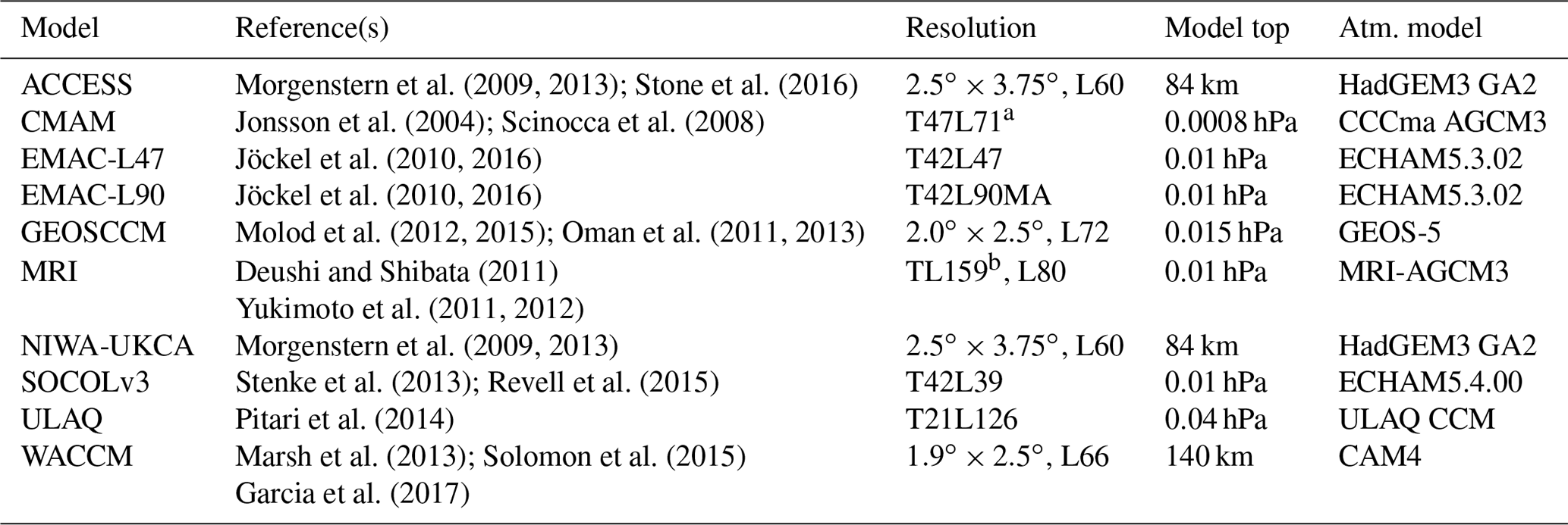
a CMAM uses a T47 spectral resolution, but physics and chemistry are performed on a linear transform grid of around 3.8∘ resolution. b The AGCM component and the chemistry-transport component of the MRI model have different resolutions (TL159 and T42, respectively), and each component is connected via a coupler. The atmospheric fields from the AGCM component are interpolated to T42 and used online in the chemistry-transport component which treats the AoA tracer.
Note that ACCESS and NIWA-UKCA, as well as EMAC-L47, EMAC-L90 and SOCOLv3 share the same atmospheric model component and that the two EMAC versions only differ in vertical resolution. ACCESS and NIWA-UKCA only differ by the fact that NIWA-UKCA is coupled to an ocean model and that the simulations are run on different platforms. The simulations we analyse are seamless simulations spanning the period 1960–2100, the so-called reference simulations REF-C2 (only r1i1p1 ensemble members). The simulations follow the WMO (2011) A1 scenario for ozone-depleting substances and the RCP 6.0 scenario (Meinshausen et al., 2011) for other greenhouse gases, tropospheric ozone (O3) precursors, and aerosol and aerosol precursor emissions. For anthropogenic emissions, the recommendation was to use MACCity (Granier et al., 2011) until 2000, followed by RCP 6.0 emissions. Out of the models used in this study, MRI, NIWA-UKCA, and WACCM have coupled an interactive ocean and sea ice module in these simulations for atmosphere-ocean interactions. In all other simulations, climate model fields (i.e. sea surface temperatures and sea ice concentrations) are imposed. A variety of different climate model data sets were used for this purpose (e.g. HadISST1 or HadGEM2 data; for details see Table S1 in Morgenstern et al., 2017). More details on the simulation setups can be found in Morgenstern et al. (2017) and in the citations given in Table 1.
2.2 Analysis methods
The methodology of this study mostly follows the companion paper Dietmüller et al. (2018). A short description of the most important concepts used here is given in the following.
Stratospheric mean AoA is defined as the mean residence time of an air parcel in the stratosphere (Hall and Plumb, 1994; Waugh and Hall, 2002). In the CCMs, the AoA tracer is implemented as an inert tracer with a mixing ratio that linearly increases over time as lower boundary condition (“clock tracer” Hall and Plumb, 1994). In some models, this lower boundary condition is global, in others only in the tropics, in NIWA-UKCA and ACCESS for example, AoA is kept at 0 in the boundary layer. AoA is then calculated as the time lag between the local mixing ratio at a certain grid point and the current mixing ratio at a reference point. This reference point, however, varies between the models (e.g. boundary layer, tropopause, 100 hPa), which could lead to inconsistencies in the AoA calculation. To avoid this, we subtract the mean AoA value of the respective model's tropical tropopause from the actual AoA value at all grid points. This means that in our analyses, AoA =0 at the tropical tropopause for all models. We perform this calculation for each time step (with monthly values) separately for the entire time period 1960–2100. Therefore, the AoA trend excludes any changes in tropospheric transport times due to the fact that the tropopause rises over time (see Vallis et al., 2015; Oberländer-Hayn et al., 2016; Abalos et al., 2017).
The residual circulation transit time (RCTT) is the hypothetical age that air would have if it only followed the residual circulation, meaning that no processes such as eddy mixing or diffusion would come into play. These RCTTs are calculated using a concept described by Birner and Bönisch (2011), by calculating backward trajectories on the basis of the Transformed Eulerian Mean (TEM) meridional () and vertical () velocities (referred to as residual velocities, available in the CCMI-1 database for the chosen models), with a standard fourth-order Runge–Kutta integration. The RCTT is then the time that these backward trajectories require to reach the tropopause from their respective starting point in the stratosphere. For more details see also Birner and Bönisch (2011) and Garny et al. (2014).
The RCTT differs from AoA because of (resolved and unresolved) mixing. In the stratosphere, this is due to the mixing of air between branches and the in-mixing of air from the mid-latitudes into the tropical pipe, which leads to recirculation of old air around the BDC branches. In global model studies, this effect has been named aging by mixing (A_mix) and is interpreted as the difference between AoA and RCTT (Garny et al., 2014; Ploeger et al., 2015a, b). However, it has to be kept in mind that the residual of AoA and RCTT does not only reflect this process alone, but actually includes resolved mixing as well as parameterized and numerical diffusion.
As a measure of the relative strength of mixing (independent of the residual circulation strength), we use the so-called mixing efficiency ϵ for analysis. ϵ is defined as the ratio of the mixing mass flux to the net residual mass flux between the tropics and the extratropics across the subtropical barrier. The net mass flux is the horizontal motion that is determined by mass continuity from vertical motion and corresponds to transport by (Garny et al., 2014). ϵ can be derived by means of the tropical leaky pipe (TLP) model (Neu and Plumb, 1999). The TLP model is a one-dimensional transport model of the stratosphere that includes advection and horizontal mixing of air between the tropics and the extratropics. It assumes two columns of well-mixed air (a tropical and an extratropical column) and can be used to quantify the strength of mixing across the subtropical barrier. If we neglect vertical diffusion (see Dietmüller et al., 2017), we can formulate an analytical solution for tropical and mid-latitude AoA. According to the TLP model, tropical AoA (AoAT) with altitude-dependent vertical velocity can thus be described as
(Neu and Plumb, 1999; Garny et al., 2014). Here, H denotes the scale height (7 km) and α(z) denotes the ratio of tropical to extratropical mass, which is approximated by
zt denotes the height of the tropical tropopause and the correction term for the altitude-dependency of the vertical residual velocity w* (an additional analytical solution term from horizontal advection; for details see Neu and Plumb, 1999; Garny et al., 2014). AoA thus depends on the advective vertical velocity (i.e. the residual velocity) and on the mixing efficiency ϵ (i.e. the amount of mixing between the tropics and the extratropics). Solving Eq. (1) for the mixing efficiency yields
Equation (3) shows that ϵ is approximately proportional to the relative increase in AoA due to mixing. For analysis, we calculate the 10 year running averages of ϵ to obtain climatologically representative values. Note that according to the concept of the TLP model, ϵ has to be viewed as a parameter valid for a given climate state in a certain model. Hence, it can vary between models and/or for different climate conditions. In the study by Garny et al. (2014), the authors nevertheless found a constant ϵ for three different climate states in one model. The tropical profiles of , tropopause height and AoA provided for the TLP model are averaged over the latitudinal bands of the models' individual vertically averaged turnaround latitudes (which are also time-dependent and calculated from v* for consistency between the models; refer to the Supplement of Dietmüller et al., 2018) and are interpolated to vertical coordinates relative to the tropopause height of each model. The mixing efficiency is then obtained by the TLP model's best fit to the CCM AoA profile. Here, the best fit is done for the altitude range from the tropopause to 32 km (details for the calculation of the mixing efficiency are given in Garny et al., 2014). According to the TLP formulation, aging by mixing (A_mix) is a function of the mixing efficiency and of the residual circulation strength:
A_mix is proportional to the mixing efficiency, but inversely proportional to the vertical velocity. A higher mixing efficiency is, e.g. connected with more air parcels recirculating (see Garny et al., 2014), thereby increasing A_mix. But the vertical velocity also controls the speed of the air parcels that recirculate. Thus, the mixing efficiency has been shown to be a useful diagnostic tool, as it does not depend on the speed of recirculation (e.g. Garny et al., 2014; Dietmüller et al., 2017).
3.1 Changes in AoA and in its components
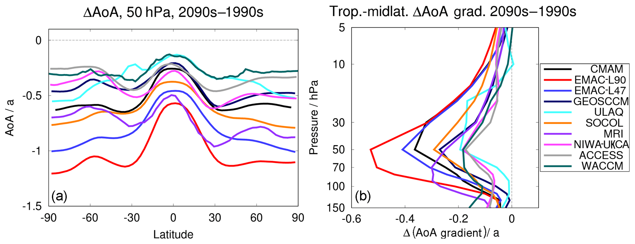
A multi-model comparison of stratospheric transport changes in the 21st century has been conducted before for the Stratosphere-Troposphere Processes and their Role in Climate (SPARC) report (SPARC, 2010). In that study, the authors showed stratospheric mean AoA of 10 chemistry–climate model simulations that took part in the CCMVal-2 (Chemistry-Climate Model Validation, Eyring et al., 2013) project. To allow a direct comparison of the simulations that were analysed in SPARC (2010) with the simulations we use here, Fig. 1 presents the same depiction of AoA differences between the 2090s and the 1990s (ΔAoA) (a) at 50 hPa and (b) as the difference between the tropics and middle latitudes as in their Fig. 5.18.
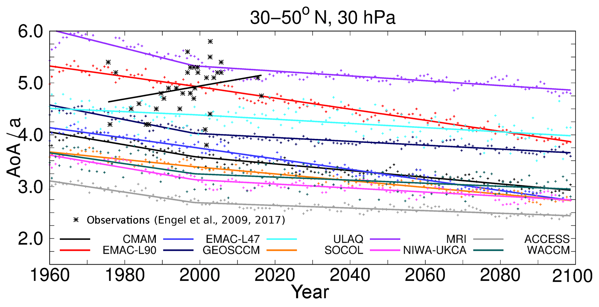
Figure 2Monthly mean AoA of the REF-C2 CCMI-1 model simulations (dots) and their linear trends at 30 hPa averaged over 30–50∘ N, as well as AoA derived from in situ measurements by Engel et al. (2009, 2017) (stars). Note that the observational AoA data are relative to ground level, while the model data have been processed to be relative to the tropopause (see main text).
The general structures of the AoA differences agree between the two model intercomparison projects. All models predict a decrease in mean AoA at 50 hPa and the smallest decrease in the tropics (Fig. 1a). A second minimum in decrease is found at 60∘ N/S and the greatest decrease is at 30∘ N/S and/or at the poles. The AoA behaviour in these regions of maximum change across the 21st century is investigated in detail by Šácha et al. (2019). They showed that these trends are related to the climatological AoA distribution, the upward shift of the pressure levels and the widening of the AoA isolines. In comparison with the CCMVal-2 models, the inter-model spread of the AoA difference is reduced in our results. However, it was the two UMUKCA (Unified Model/U. K. Chemistry Aerosol) models that led to the large spread in the SPARC report and are not part of our analysis. However, NIWA-UKCA and ACCESS are the direct successors to the UMUKCA models and these range in the lower end of AoA changes here. The ULAQ model has changed from a very large latitudinal ΔAoA amplitude to a rather small one from CCMVal-2 to CCMI-1. Other models that appear in both studies do not show large changes. The EMAC model was not included in the SPARC report. With a higher vertical resolution (47 to 90 levels in the vertical), the EMAC model tends to simulate larger ΔAoA and thereby detaches from the bulk of the other model simulations. Consistent with this, Revell et al. (2015) show that in the SOCOLv3 model, AoA also gets on average 1 year older when the model is run with 90 layers in the vertical (instead of 39) because of less vertical diffusion. All the statements above also count for Fig. 1b and the tropical to middle-latitude AoA differences with altitude (Fig. 1b).
To visualise AoA and its trends of the model simulations and their inter-model differences, we present the annual mean AoA data of the 10 CCMI-1 model simulations in Fig. 2. Moreover, the piecewise linear regression of AoA for the periods 1960–2000 and 2000–2100 is presented. These two periods were chosen because the year 2000 marks a change in stratospheric dynamics, which is due to the reversal in signs of ODS and ozone trends as a consequence of the Montreal Protocol (see Morgenstern et al., 2018; Polvani et al., 2018). We chose the 30 hPa pressure level and an average between 30 and 50∘ N, because the observation-based data from Engel et al. (2009, 2017) are from that region too. These data and their linear regression are included in the figure as well; they show a non-significant positive AoA trend of 0.15±0.18 years decade−1.
The absolute AoA values differ strongly among the models. For the first three decades of the simulations (i.e. the mean from 1960–1990) the values range between 5.52 years in the MRI model and 3.18 years in the ACCESS model simulation. This topic had already been discussed, for example in SPARC (2010) and in Dietmüller et al. (2018). Analysing the hindcast simulations of the CCMVal-2 and the CCMI-1 projects, Dietmüller et al. (2018) showed that it is mainly the mixing rather than the residual circulation that causes the large AoA spread and that this is likely linked to the different resolutions of the model simulations.
All the model simulations show a clear negative trend over time across the first, as well as across the second period. The in situ measurement-based observations (Engel et al., 2009, 2017), in contrast, display a positive, but not significant, trend for the last couple of decades. A similar behaviour to the in situ measurements can also be found in satellite-based observations, for example, in Haenel et al. (2015), although for a shorter time series (2002–2012). A number of studies have investigated this discrepancy (see e.g. Engel et al., 2009; Garcia et al., 2011; Ploeger et al., 2015a) and many reasons have been discussed to resolve this contradiction (e.g. effect of mixing in models, sparse sampling of observational data, differences in changes between deep and shallow BDC branches), but a viable explanation is still missing. In the present study, however, we do not discuss this issue any further, but rather focus on the analysis of the negative AoA trends in the model simulations. The models may agree in predicting a decrease in stratospheric AoA, but they do show large differences in the strength of this trend (σ(ΔAoA)=0.18 for μ(ΔAoA)=0.54; see below for ΔAoA). Also, the trends between the two periods (1960–2000 and 2000–2100) differ. Most models show a stronger trend between 1960 and 2000, only the two EMAC simulations have a stronger trend in the second period and in SOCOLv3 the trend almost remains constant. Note, however, that EMAC has a negative bias in ODSs, because the replacement products were not taken into account as F11 or F12 equivalents. This can possibly explain why the AoA trend is weaker between 1960 and 2000. Several studies (e.g. Austin and Li, 2006; Oberländer-Hayn et al., 2015; Oman et al., 2009; Polvani et al., 2017, 2018; Morgenstern et al., 2018) have recently pointed out the importance of the role of ODSs for the trends in stratospheric dynamics. ODSs act as both, radiatively active greenhouse gases and chemically active gases controlling ozone depletion and recovery. During the period between 1960 and 2000, ODSs increase and thus act in concert with GHGs to cause an AoA decrease. Thereafter, however, ODSs decrease over time, which means that with respect to AoA trends, the ODS trend works against the trend in the continuously rising GHGs. This can possibly explain the weaker trend in the second period in most models. Due to this change in dynamical properties around the year 2000, an analysis of the trends across the entire period from 1960 to 2100 cannot be conducted without mixing-up various dynamical effects. The first period is relatively short for robust analyses of mixing trends and in the second period, two mechanisms work against each other, so that in most models, the trends are rather small. In the following, we therefore analyse the differences between the periods 1970–1990 and 2080–2100. Based on the sensitivity simulations in Polvani et al. (2018), which shows that the change in the slope in the year 2000 is due to ODSs, this allows the capturing of the GHG effect alone. At the end of the 21st century, ODS mixing ratios have declined to similar values as between 1970 and 1990 in the simulations. We do not start our investigation at 1960 due to the calculation method of RCTTs and ϵ, which are available only from 1970 onwards.
Table 2The climatologies and differences of AoA (averaged over 100–10 hPa and 90∘ S–90∘ N), the mixing efficiency ϵ, and tropical upwelling at 70 hPa. The 1970 means are averaged over 1970–1990 and the 2100 means are averaged over 2080–2100. Δ means the difference between the two latter (climate states 2100 minus 1970). Note that rounding can lead to seemingly wrong Δ values here.
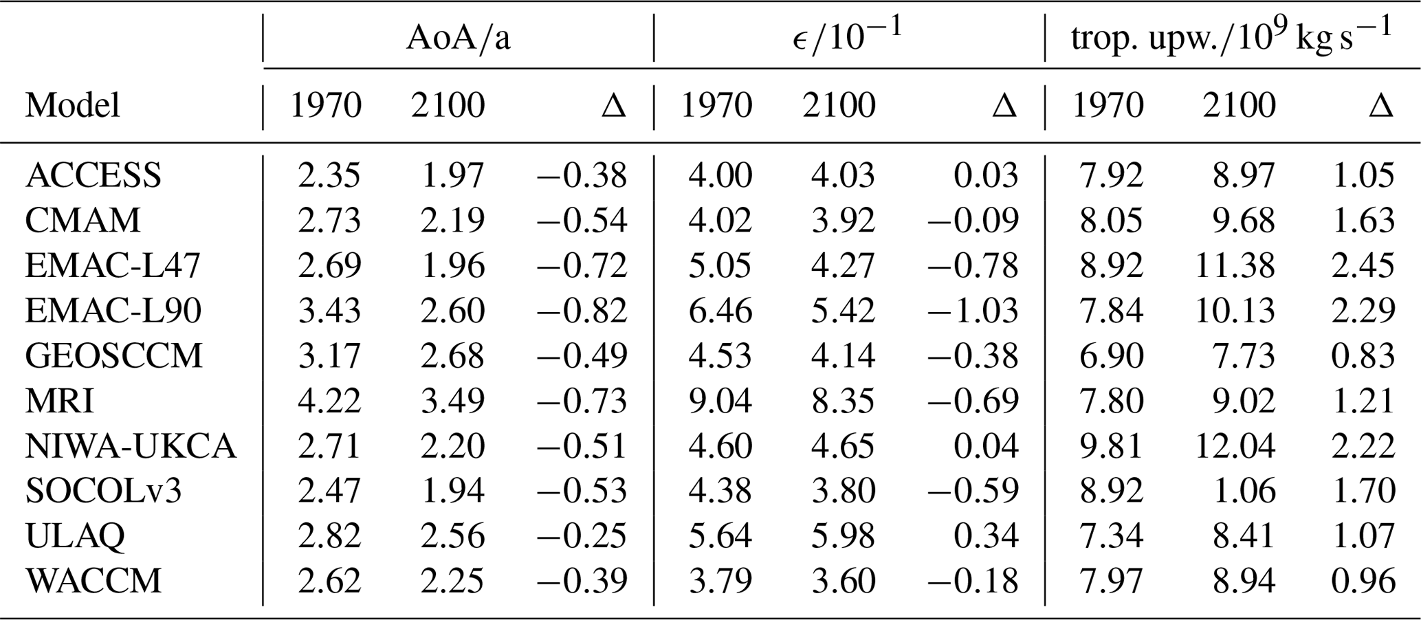
Table 2 provides an overview over mean AoA, ϵ and tropical upwelling (at 70 hPa) averaged between 1970 and 1990 (denoted as 1970) and between 2080 and 2100 (denoted as 2100) and their differences (Δ) for the 10 CCMI-1 REF-C2 model simulations. For consistency with ϵ and tropical upwelling (which are global values), we here averaged AoA globally (90∘ S–90∘ N) and over 10–100 hPa, which means that these AoA values are not comparable with those in Fig. 2. Table 2 will be used to explain and confirm some of the results throughout the paper.
Figure 3 shows the linear AoA changes, along with the ratio of the RCTT change to the AoA change (ΔRCTT ∕ ΔAoA) for a model intercomparison of the zonal mean structure of the differences. Moreover, the contour lines show the climatologies of the 1970–1990 period of the simulations for AoA and for the RCTT ∕ AoA ratio, respectively. The ΔRCTT ∕ ΔAoA ratio provides the possibility to linearly separate ΔAoA into its contributions from residual transport and aging by mixing (A_mix). Specifically, values between 0.5 and 1 signify a domination of residual transport changes (reddish), while values between 0 and 0.5 mean that ΔAoA is controlled by A_mix variations (blueish). Values above 1 mean that the A_mix difference is positive and values below 0 mean that ΔRCTT is positive (assuming a negative ΔAoA).
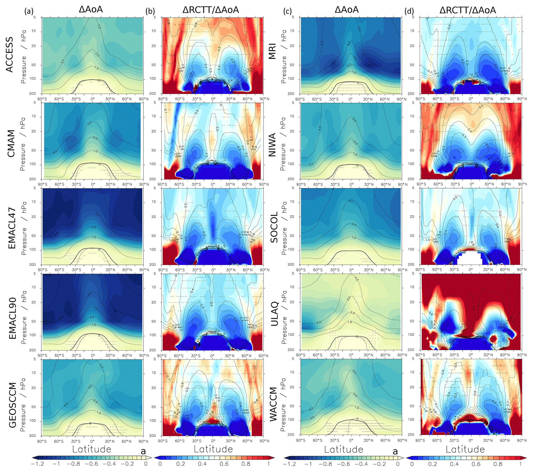
Figure 3ΔAoA (columns a and c) and ΔRCTT ∕ ΔAoA (columns b and d) between the periods 1970–1990 and 2080–2100 for the CCMI-1 REF-C2 simulations in colour. The contour lines show the respective 20-year climatologies from 1970–1990. Stippled regions mark where the significance of the difference is below the threshold of 95 %.
In most models, a quite similar ΔAoA pattern can be seen. Relatively small ΔAoA dominates the tropical pipe where young air is prevalent and the differences increase with higher altitudes and latitudes. Several model simulations (ACCESS, CMAM, MRI, NIWA-UKCA), however, show their maximum ΔAoA in the lower stratospheric middle latitudes. This feature is connected with the climatological AoA gradient, the upward shift of the circulation and the decrease in RCTT and A_mix in Šácha et al. (2019). The two EMAC simulations show the largest ΔAoA throughout the stratosphere and the ULAQ model the weakest. Moreover, ULAQ is the only model that shows a pronounced hemispheric asymmetry, with stronger differences in the SH. These general ΔAoA patterns were also found in the multi-model study by Butchart et al. (2010) who analysed 11 21st century model simulations that were performed for WMO (2006). Most models also agree in the ΔRCTT ∕ ΔAoA pattern. Strong A_mix-dominated ΔAoA can be seen in the middle-latitude lower stratosphere and the residual circulation dominates ΔAoA mainly in the tropical pipe as well as in the downwelling branches in the high latitudes. Some model simulations hardly show any regions where the differences of residual transport accounts for less than 50 % of ΔAoA throughout the stratosphere, even in the upwelling and downwelling branches (EMACL47, EMACL90, GEOSCCM, SOCOLv3). Other models (GEOSCCM, ACCESS, NIWA-UKCA, WACCM) show distinct upwelling and downwelling branches. This indicates that ΔAoA is not influenced much by ΔA_mix in these particular regions. The NIWA-UKCA model shows a clear separation between aging by mixing and residual circulation dominated regions, and in the ULAQ model, the ΔA_mix is slightly positive in most parts of the stratosphere (i.e. ΔAoA ∕ ΔRCTT >1). Altogether, these results suggest that changes in aging by mixing have a major impact on ΔAoA. This brings us to further analyse A_mix changes as well as the mixing efficiency and to discuss possible reasons for their variations.
3.2 Coherences between the components
Figure 3 suggests that most of the ΔAoA is determined by aging by mixing changes. However, A_mix itself depends on RCTT (see Eq. 4) and is therefore not an independent measure for separation of the processes. AoA changes are commonly attributed to changes in the residual circulation (e.g. Austin and Li, 2006). In the climatologies, the tropical upwelling (as calculated via integration of v* between the turn-around latitudes; see e.g. Okamoto et al., 2011) in the 70 hPa pressure level has been shown to be a good measure for the strength of the residual circulation throughout the stratosphere (see Dietmüller et al., 2018). To see if this relationship holds true for ΔAoA in our set of the CCMI model simulations, we present in Fig. 4 the inter-model correlations between ΔAoA and ΔRCTT, as well as between the ΔAoA and the differences in tropical upwelling in 70 hPa. These correlations are calculated across the 10 model simulations for each grid point separately. Note that for this, data from each model were interpolated to the resolution of the grid of the highest horizontal model grid resolution.
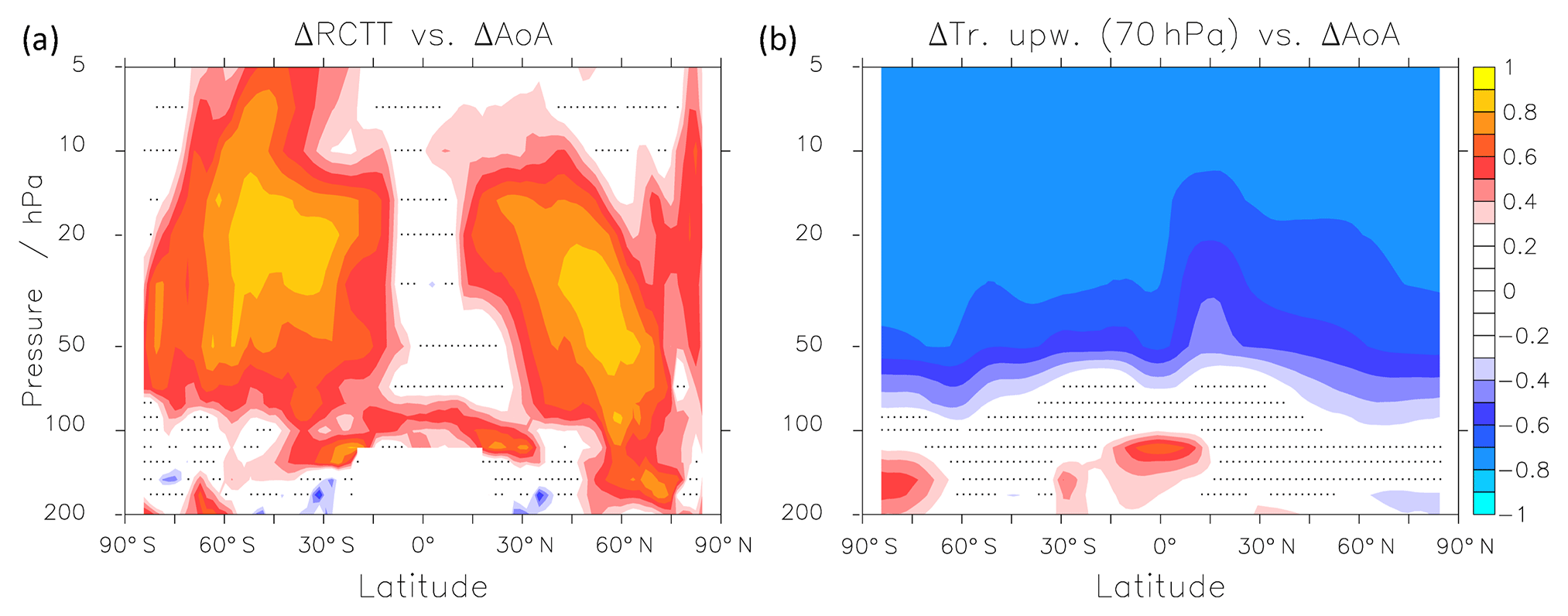
Figure 4Inter-model correlations (a) between ΔAoA and ΔRCTT and (b) between ΔAoA and Δtropical upwelling at 70 hPa as calculated over the individual turnaround latitudes of the respective model. Stippled regions show where the significance level of the correlation is below the threshold of 5 %.
A high correlation between ΔRCTT and ΔAoA (Fig. 4a) can only be seen in the middle to high latitudes between around 70 and 10 hPa and low or no correlations in the other regions. In the upwelling region in the tropics this is particularly surprising since AoA should be controlled by the upwelling speed there. However, this connection apparently is not local. The correlations between ΔAoA and Δtropical upwelling (Fig. 4b) are high in the entire stratosphere above around 70–50 hPa. This reflects a clear connection between tropical upwelling and AoA, particularly in the deep branch. A stronger tropical upwelling generates a faster circulation and hence a decrease in AoA. The strengthening of tropical upwelling can be explained by an enhancement of the subtropical jet streams following from upper tropospheric warming and lower stratospheric cooling (see e.g. Lorenz and DeWeaver, 2007; Randel et al., 2008; Butchart, 2014) and was linked with the upward shift of the tropopause by Vallis et al. (2015) and Oberländer-Hayn et al. (2016). The rather patchy picture of the ΔRCTT vs. ΔAoA correlations suggests that the link between the residual circulation and AoA cannot be expected to be local, but rather of remote nature. It is mainly the ascent of air in the tropics that determines the ΔAoA-dependency on the residual circulation. The upwelling and downwelling regions in particular do not correlate well in Fig. 4a, although ΔAoA is clearly dominated by the changes in transport in those regions (see Fig. 3).
Dietmüller et al. (2018) showed that the climatological inter-model AoA spread in the CCMVal-2/CCMI-1 hindcast simulations can mostly be explained by model differences in mixing efficiency and only to some extent by differences in residual circulation. Hence, we now focus on the model trends (and differences between the two periods) in mixing efficiency and on the processes that are responsible for its changes. ϵ provides information on the models' relative strengths in mixing at the tropical barriers as a vertically integrated measure (see Sect. 2.2 for calculation method). Figure 5 shows the time series of the mixing efficiency of each model for the REF-C2 simulation period and, as in Fig. 2, the piecewise linear regressions for the time before and after the year 2000 are included. Note that due to the calculation of the 10-year moving average of ϵ, the first 10 years cannot be assessed here. For a more quantitative view, the Δϵ and the climatological ϵ of the two simulation periods are also presented in Table 2.
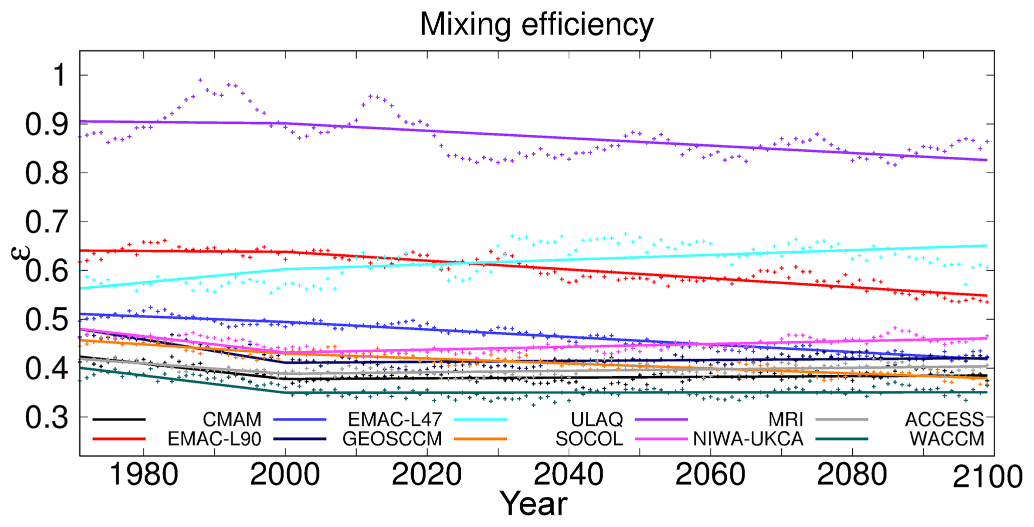
Figure 5Mixing efficiencies ϵ of the REF-C2 CCMI-1 model simulations and their piecewise linear regression for the periods 1970–2000 and 2000–2100.
The climatological ϵ of the first 20 REF-C2 simulation years show similar values as the REF-C1 (CCMI-1 reference hindcast simulations from 1960–2011; for details see Morgenstern et al., 2017) values that were shown in Dietmüller et al. (2018). In this period, the main differences between the REF-C1 and the REF-C2 simulations are the sea surface temperatures and the sea ice distribution. Only MRI shows a somewhat higher mixing efficiency in the REF-C2 simulation (∼50 %). The multi-model mean of this climatological ϵ is 0.52 %±31 %. This agrees well with the value (0.58 %±32 %) that was found for the REF-C1 simulations (for ϵ calculated at the turnaround latitudes) by Dietmüller et al. (2018). Across the whole simulation period, the mixing efficiency decreases over time in most models. However, the sign of the trend often changes between the two periods. For example in MRI and in EMAC-L90, ϵ is at first almost constant and then it decreases; and in GEOSCCM and CMAM, ϵ at first decreases and in the later period it rises. Only the ULAQ model shows a positive trend in both periods. For the reasons we mentioned above (counteracting influence of GHGs and ODSs), we now again discuss the differences between the start and the end of the simulations to filter out the direct effect of ODSs on stratospheric dynamics. The ϵ values for the periods in question, as well as their differences are provided in Table 2. The ACCESS and the NIWA-UKCA model (the two models with the HadGEM atmospheric model component) show a slight positive Δϵ and the only model with a strong positive Δϵ is ULAQ. The fact that the mixing efficiency is not constant over time means that the absolute mixing strength does not change proportionally with the residual circulation. This is in contrast to the results of Garny et al. (2014), who found a nearly constant ϵ when comparing three GCM simulations with different climate states. However, Garny et al. (2014) also make clear that it would not be surprising if ϵ varied over the course of climate change simulations, because the properties of the mixing barriers can also change over time. The mechanisms for the mixing changes are diagnosed using the potential vorticity gradient in Sect. 3.4. Next, we investigate if ΔAoA is also linked to variations in mixing efficiency, and not merely to residual circulation changes. For this, Fig. 6 shows the inter-model correlations (correlations across the 10 model simulations) between the local ΔAoA and the models' differences in mixing efficiency.

Figure 6Inter-model correlations between ΔAoA and Δϵ. Stippled regions show where the significance level of the correlation is below the threshold of 5 %.
Figure 6 shows a clear link between ΔAoA and Δϵ above around 100–70 hPa, with correlation coefficients mostly ranging between 0.8 and 0.9. This reflects that a decline in mixing efficiency leads to a decrease in AoA, because there is less recirculation of air around the BDC. Only in the region around the Antarctic polar vortex is the correlation generally somewhat weaker. This may be due to changes in the polar vortex strength or position in the various models, which cannot be reflected in the (sub)tropical measure ϵ.
A_mix is connected with the mixing efficiency, but it also depends on the residual circulation. A higher or lower mixing efficiency causes more or less recirculation, which increases or decreases aging by mixing, respectively, and the RCTT controls the transit times of the air parcels that recirculate. Overall, we can again conclude that ΔAoA in climate models is connected with changes in both, mixing and residual transport. Most of the ΔAoA that is connected with residual transport can be attributed to tropical upwelling changes, at least for the deep BDC branch. This is caused by a climate change induced strengthening and/or upward shift of the subtropical jet streams (see e.g. Randel et al., 2008; Shepherd and McLandress, 2011; Butchart, 2014; Oberländer-Hayn et al., 2016). The differences in mixing between future and past climate, however, have not been analysed in detail before. Therefore, we investigate the overall effect of mixing on the BDC changes in the remainder of the paper.
3.3 Impact of the mixing changes
To quantify the impact that changes in mixing efficiency have on ΔAoA in the simulations, we again apply the TLP model, now by using , the tropopause height and a given ϵ to calculate the RCTTs and AoA (see Eq. 1). We then compare the AoA and RCTT climatologies of the two periods 1970–1990 (1970) and 2080–2100 (2100). Figure 7 shows the tropical AoA and RCTT profiles (calculated with the TLP model) of these climatologies exemplarily for the EMAC-L90 model simulation. Moreover, two hypothetical AoA profiles (AoA′ and AoA*) are included in the figure (both for 2100). AoA′(2100) (gray line in Fig. 7) displays the AoA climatology for 2100 with the A_mix fixed to the value of 1970, it is calculated by AoA. The difference between AoA(1970) and AoA′(2100) then yields the AoA change that is caused by the RCTT change only (without a change in A_mix). The AoA*(2100) (black line in Fig. 7) profile displays the AoA climatology of the 2100 climate state by keeping the mixing efficiency constant at the value of 1970. We calculate this quantity by using ϵ(1970) in Eq. (1) for the AoAT(2100) calculation, thus it represents how much influence the change in ϵ has on ΔAoA (in contrast to the change in residual circulation only).
The RCTT and AoA climatologies of the EMAC-L90 simulation of both climate states show that RCTT explains about one-third of the AoA values. The difference (about two-thirds) is caused by aging by mixing (see Fig. 7). This ratio had already been found in Dietmüller et al. (2018) for the CCMVal-2 and CCMI-1 hindcast simulations. AoA′ reveals that for EMAC-L90 this ratio roughly also accounts for the differences between the periods. The AoA difference between 2100 and 1970 is subdivided by AoA′ into about one-third the share of RCTT difference and two-thirds of A_mix. This ratio can also be estimated from Fig. 3 for the EMAC-L90 simulation. However, as already stated above, the A_mix change also includes some RCTT change (see Eq. 4), which implies that this is not a clear separation of the mechanisms.
The difference between AoA*(2100) and AoA(2100) reflects the impact of Δϵ on AoA. In the given example of the EMAC-L90 model, the fractional impact of the mixing efficiency change on the AoA difference is 29 %±4 % as calculated between 2.5 and 25 km above the tropopause. This value varies considerably among the 10 models, Table 3 provides an overview.
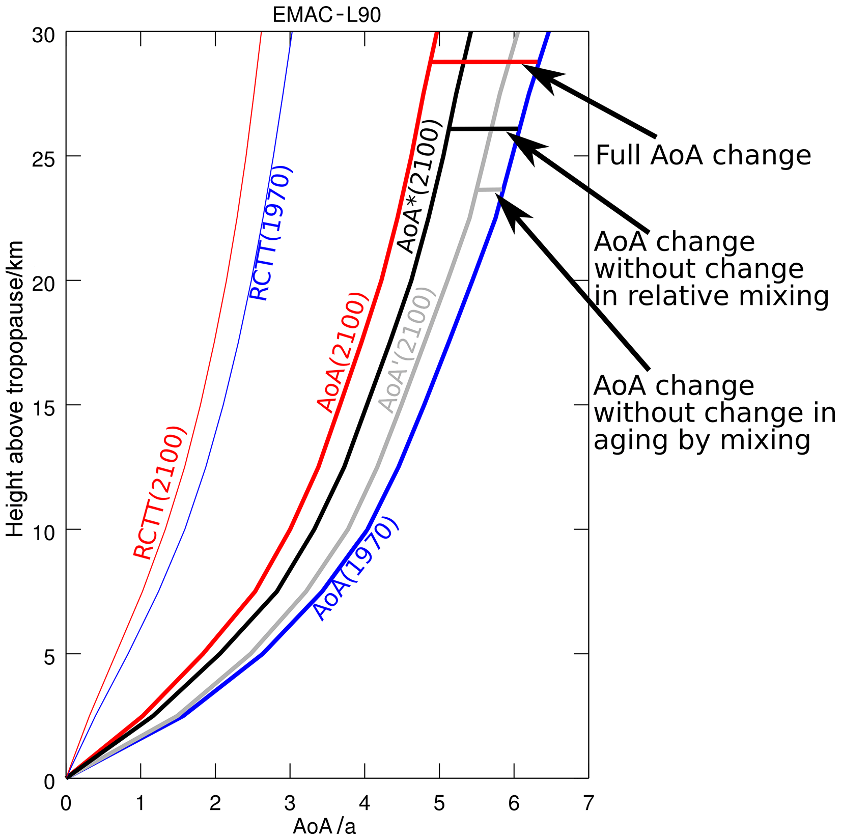
Figure 7AoA and RCTT of the EMAC-L90 simulation for the two periods 1970–1990 and 2080–2100. Also included are a hypothetical AoA* that displays the AoA at the end of the simulation but with the mixing efficiency of the beginning of the simulation and AoA′, a hypothetical AoA that represents AoA at the end of the simulation with the A_mix of the beginning (see main text for details). The difference between AoA and RCTT resembles the influence of aging by mixing. The difference between AoA and AoA* (both 2080–2100) resembles the influence of the mixing efficiency changes on ΔAoA and AoA′ represents the subdivision of the AoA difference between the two climate states into the influences of A_mix and RCTT changes.
Table 3Contribution of the relative change in mixing (i.e. the mixing efficiency changes) to the overall ΔAoA between the periods 2080–2100 and 1970–1990 calculated between 2.5 and 25 km above the tropopause.
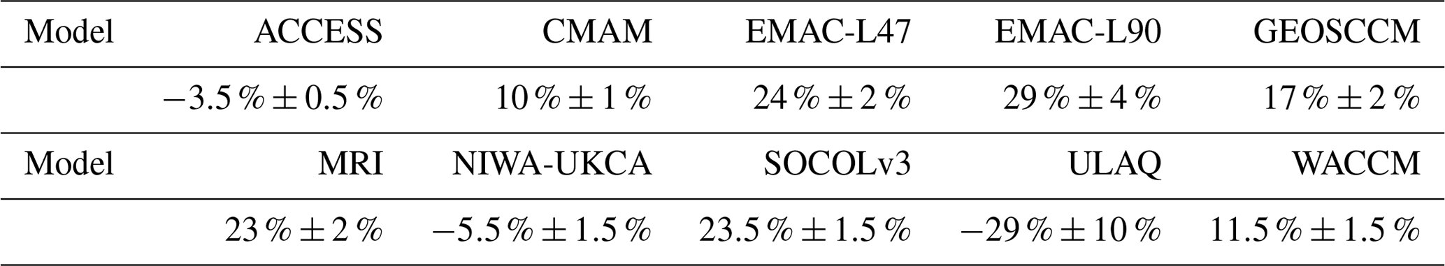
NIWA-UKCA, ACCESS and ULAQ show a negative fractional impact of mixing efficiency on AoA changes. These are the three models that also show a positive Δϵ (see Table 2). In contrast to the other models, the mixing efficiency therefore leads to an AoA increase over time. The negative ΔRCTT therefore accounts for more than the entire negative ΔAoA to compensate for the effect of the ϵ change. With less than 5.5 % and 3.5 %, NIWA-UKCA and ACCESS have the lowest contribution of Δϵ on the AoA change and with up to 29 %, ULAQ and EMAC-L90 have the largest. The other models have a contribution of Δϵ on ΔAoA between 10 % and 29 %, the multi-model mean is 10.4 % (σ=18.3 %). It is reasonable that a large Δϵ leads to a high percentage of the ϵ-share on ΔAoA. The correlation coefficient between the two values is 0.83. This makes clear that the change in mixing efficiency does have a considerable impact on ΔAoA, as it could already be assumed from the high inter-model correlations between the two quantities (Fig. 6). Due to the large model spread in Δϵ, however, this impact bears large uncertainties. Next, we quantify the impact of Δϵ on the model spread in ΔAoA.
To analyse the share of Δϵ on the AoA model spread, we again use the TLP model-calculated values of ϵ, α(z), Tcorr and RCTTT. These quantities are taken to calculate tropical AoA by
as an average between 100 and 10 hPa. As above, this calculation is performed for each model for the two periods, so that . Using ϵ(1970) to calculate AoAT(2100) in Eq. (1) provides AoA(2100) and thus provides the AoA difference without any changes in ϵ. Figure 8 displays the model distribution of ΔAoA with (blue) and without (red) a changing mixing efficiency.
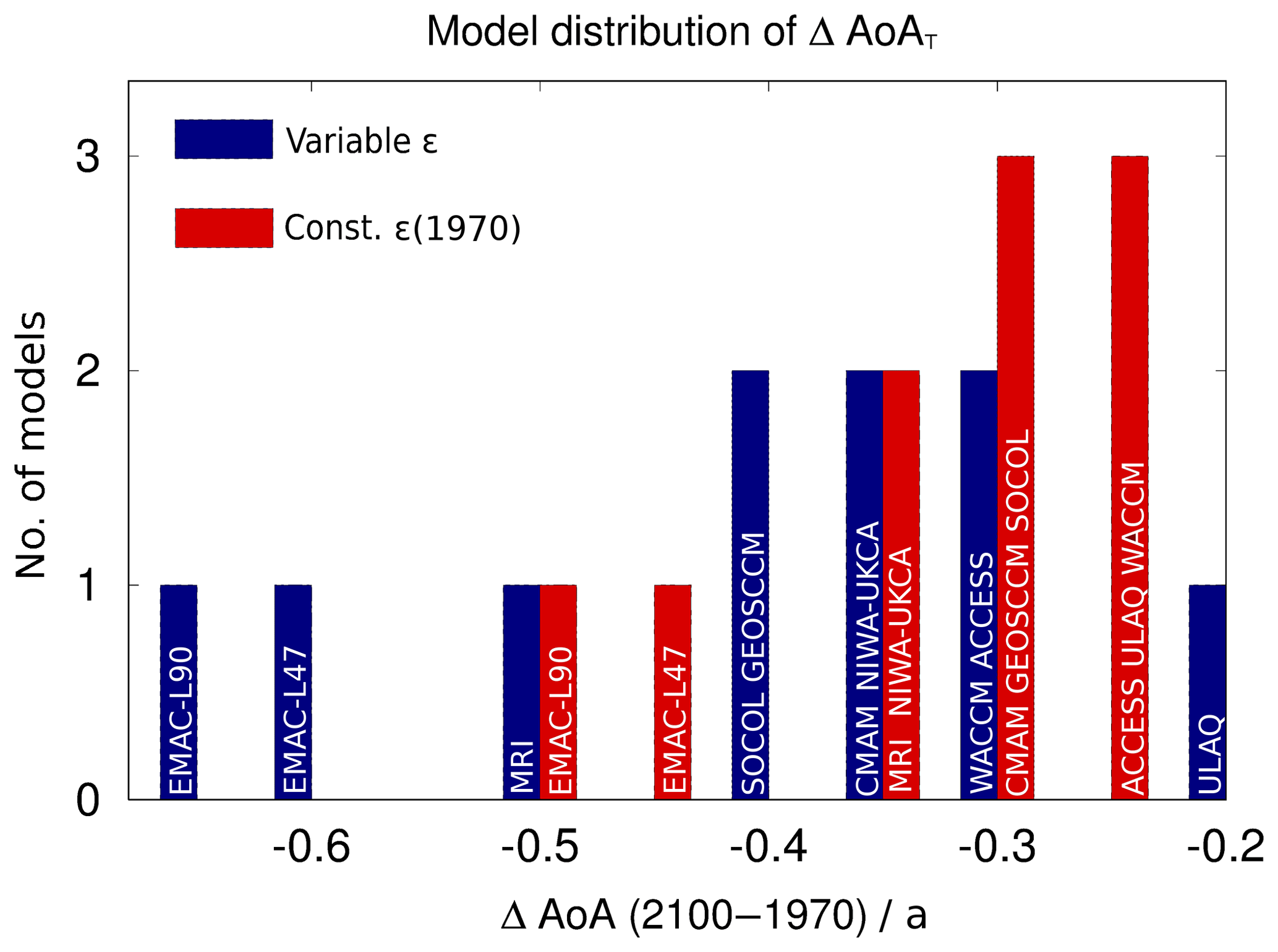
Figure 8Model distribution of the tropical AoA difference (averaged from 100 to 10 hPa) between the two periods 1970–1990 and 2080–2100 calculated after Eq. (5) with a variable ϵ (blue) and with a constant ϵ(1970) (red).
Figure 8 clearly shows that when ϵ is kept constant, first, ΔAoA generally decreases (in absolute values) and second, the model spread of ΔAoA is considerably reduced (from 0.35 to 0.22 years). This reflects that the mixing efficiency changes lead to strong variations in AoA. When ϵ is held constant, for models with negative Δϵ, ΔAoA is reduced (in absolute values) (see for example EMAC) and ΔAoA is enhanced for models with positive Δϵ (see for example ULAQ). The model range decreases here because being the model with the largest ΔAoA, EMAC-L90 has a negative Δϵ and ULAQ, the model with the lowest ΔAoA has a positive Δϵ. A large or small (negative) Δϵ causes a large or small ΔAoA. From this analysis, we can conclude that |ΔAoA| generally increases through the changes in mixing efficiency (by 10.4 % as multi-model mean) and that Δϵ leads to a larger model spread in the AoA changes (Δϵ increases the ΔAoA model range by about 37 %).
Now, the question remains what the reasons for the changes in relative mixing strength are, or why ϵ changes in the course of climate change simulations. In the next section, we will explore an explanation for this by analysing various dynamical fields.
3.4 On the mechanism of mixing changes
The relation between residual circulation and mixing determines the mixing efficiency and changes therein. To study possible dynamical reasons for the changes in mixing efficiency, the relation of wave driving, the residual circulation and mixing is analysed in the following based on the Transformed Eulerian Mean (TEM) momentum equation. This analysis is similar to that presented in Garny et al. (2014), but here we use the quasi-geostrophic (QG) formulations on pressure levels (on which the CCMI data are available). We present and analyse multi-model mean (MMM) diagnostics to provide a general picture for the entire subset of CCMI-1 model simulations. Unless otherwise stated in the text, the individual models qualitatively agree fairly well in these diagnostics. The fields of the individual models can be found in the Supplement. Figure 9 shows the differences between the two periods (1970–1990 and 2080–2100) overlaid with the MMM climatologies of the first period of zonal winds, Eliassen–Palm flux divergence (EPfd), v*, the meridional potential vorticity gradient (∂PV ), as well as Kyy and . The calculation of Kyy and the meanings of these variables will be explained below. Due to data availability, not all models could be included in these MMMs. For SOCOL and ULAQ, the EPfd fields were not available, hence, for consistency, all MMMs are based on the remaining eight other models only.
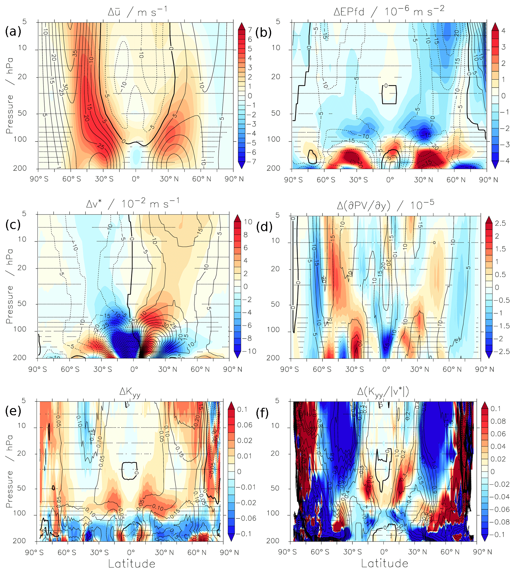
Figure 9Multi-model mean differences (Δ) of (a) the zonal wind , (b) the EP flux divergence, (c) the meridional residual circulation v*, (d) the meridional PV-gradient (), (e) the diffusivity coefficient Kyy and (f) the ratio between the periods 1970–1990 and 2080–2100 of the eight (see main text) CCMI REF-C2 simulations. The contour lines show the multi-model mean climatology of the first period of the respective quantity. Stippled regions show where the statistical significance of the difference is below the threshold 95 %.
The mechanism of the residual circulation increase in the lower stratosphere is well understood (e.g. Shepherd and McLandress, 2011). It follows the upper tropospheric temperature increase that leads to an upward shift and increase of the zonal mean winds. This can be seen in Fig. 9a, which shows the MMM differences of the zonal mean wind between the two time periods. Subsequently, the critical layers that allow for wave propagation shift to higher levels. This becomes evident from Fig. 9b. There, a region of strongly negative ΔEPfd (enhanced wave dissipation) can be seen between about 100 and 50 hPa (with maxima around 70 hPa) and positive differences (less wave dissipation) can be found between around 200 and 150 hPa. The enhanced wave dissipation in the lower stratosphere leads to amplified poleward residual transport, which reflects in Δv* (Fig. 9c).
However, as shown in the sections above, transport changes in a future climate are not only due to this increase in residual transport, but also due to changes in eddy mixing. The EPfd (∇⋅F) not only drives the residual circulation, but it is also related to eddy mixing of potential vorticity q. Under the quasi-geostrophic (QG) approximation and neglecting parameterized (gravity) wave forcing, this can be formulated as
where v′ and q′ denote the deviation of their zonal means and , respectively. Note that due to data availability, we show the full EPfd fields in Fig. 9 and not the QG EPfd. Note also, that strictly speaking this relation holds true on the beta plane (Andrews et al., 1987), or approximately on isentropic surfaces, i.e. on Θ levels, on which mixing takes place. Therefore, the quantity may be somewhat distorted on the pressure levels presented here. This may lead to differences in the quantities, however, not qualitatively different conclusions in the following. Commonly, a flux–gradient relationship is assumed for the eddy PV flux, so that , with the diffusivity coefficient Kyy. ∂qy is the gradient of the QG PV (see e.g. Edmon et al., 1980; Cohen et al., 2014) with
Similarly to in Abalos et al. (2016), we calculate the diffusivity coefficient Kyy as
This relation states that horizontal eddy mixing is proportional to the EP flux divergence, and inversely proportional to the meridional PV gradient. Thus, a weak PV gradient indicates strong mixing, while a strong PV gradient acts as barrier to mixing, and thus mixing is suppressed.
The MMM differences show that next to the enhanced wave dissipation in most of the stratosphere ( increases); the PV gradient also increases from the subtropics to mid-latitudes (see Fig. 9d) due to the strengthened winds. Thus, Kyy tends to be enhanced due to increased wave dissipation, but reduced due to the increased PV gradient. As seen in Fig. 9e, the diffusivity changes are dominated by the increase in wave dissipation in the lower stratosphere (between around 100 to 50 hPa in both hemispheres) and by the decrease in wave dissipation below. This means that the vertical shift of EP flux convergence is reflected in ΔKyy, or in other words, that the region of strong mixing is shifted upward and the absolute strength of mixing increases in the lower stratosphere. At higher altitudes, the PV gradient contributes more strongly to Kyy, and in the SH mid-latitudes, the mixing strength Kyy even decreases despite enhanced wave dissipation due to the strongly enhanced PV gradient. In the NH, ΔKyy is smaller and mostly positive in the MMM. However, it should be noted that in the lower stratospheric subtropics in particular, which is the region of the climatological maxima of orographic gravity wave drag, the QG assumption can be misleading due to the neglect of parameterized wave drag.
The mixing efficiency derived from the AoA data represents the relative strength of mixing, i.e. the ratio of the mixing mass flux to the residual meridional mass flux. The mixing mass flux is proportional to the mixing velocity that can be expressed as for a given horizontal length scale L. Thus, the ratio of mixing vs. residual mass flux can be approximated as
Given a constant length scale L, the mixing-to-mean-advection ratio is proportional to . As shown above, residual transport as well as mixing increases in most regions (Fig. 9c and e). Figure 9f, however, shows that the ratio decreases in large parts of the stratosphere. This means that mixing increases less strongly (or even decreases) than residual transport. Only in the (sub-)tropical lower to mid-stratosphere, the relative mixing strength increases. The changes in mostly reflect the inverse change in the PV gradient, because the mixing diffusivity is inversely related to it. Note that if assuming , the ratio equals ; i.e. the ratio is only related to the PV gradient. Changes in are overall similar to changes in (not shown), except for some details that might be related to the simplification of the equations and/or to the neglect of parameterised wave drag (i.e. small scale gravity wave drag).
Overall, this analysis suggests that enhanced wave dissipation (caused by the zonal mean wind increase; see Shepherd and McLandress, 2011) amplifies the residual circulation as well as mixing, particularly in the lower stratosphere. However, the zonal mean wind changes also cause changes in the meridional PV gradient, and the stronger PV gradients act to inhibit mixing. Therefore, mixing increases less strongly than residual transport does, which explains the decrease in the mixing efficiency in the future (see Sect. 3.2).
However, as shown in Sect. 3.2, the mixing efficiency does not decrease in all models. In Fig. 10, the mean in the region of the subtropical barrier averaged between 20 and 40∘ S, and between 20 and 40∘ N is shown with altitude for the subset of eight CCMI-1 model simulations.

Figure 10 (mean of 2080–2100 minus mean of 1970–1990) with altitude averaged between (a) 20∘ S and (b) 40∘ S, as well as between 20 and 40∘ N for eight of the CCMI model simulations.
is larger in the SH compared to the NH, in particular at higher altitudes. This is due to the acceleration of the Antarctic polar vortex (Fig. 9a) that leads to an increase in ∂qy (Fig. 9d), thereby reducing effective mixing. In most models, is negative within these latitudes throughout the stratosphere in the SH as well as in the NH. Between 20 and 50 hPa there are only two exceptions, namely NIWA-UKCA and ACCESS in the NH, those two models that also have a slight positive Δϵ (see Table 2). Moreover, the two EMAC model versions, which have the largest Δϵ also show the largest , in both hemispheres. Although we cannot find a clear inter-model correlation between Δϵ and here, these are strong indications of a link between the two quantities.
Hence, the inter-model differences in mixing efficiency changes are consistent with differences in the relative rate of change in mixing to residual transport. The differences in changes between the models appear to be related to structural differences in zonal wind changes; i.e. the models with an increasing mixing efficiency (namely NIWA-UKCA and ACCESS) simulate zonal wind increases in the NH at higher latitudes than other models. As a consequence, the PV gradient also increases at higher latitudes, so that mixing increases more strongly in the region of the subtropical barrier (see figures in Supplement). Our approximations, as well as the limited number of models, do not warrant a robust conclusion from inter-model correlations. However, the results shown here suggest that the mixing efficiency changes, as well as the inter-model spread, are consistent with changes in the relative mixing strength due to changes in the background PV gradient.
In the present study, we analyse the AoA differences of 10 CCMI-1 (Morgenstern et al., 2017) climate prediction simulations between the two periods 1970–1990 and 2080–2100. In agreement with previous model studies (Butchart et al., 2010; SPARC, 2010), AoA decreases over time in all model simulations. The smallest differences are consistently found in the tropics and the largest in the extratropical lower stratosphere, but the magnitude of the changes varies vastly among the models (σ(ΔAoA)=0.18 for μ(ΔAoA)=0.54). Our investigation focuses on the reasons for this negative ΔAoA (AoA(2080–2100)-AoA(1970–1990)) in the analysed model simulations, as well as on the causes for the large model differences in ΔAoA.
Linear separation of ΔAoA into changes by aging by mixing (A_mix) and changes by residual circulation (Birner and Bönisch, 2011; Garny et al., 2014), shows that the contribution due to ΔA_mix dominates in all models. In particular, the influence of ΔA_mix controls almost the entire changes in AoA in the subtropical lower stratosphere. ΔRCTT is important in the tropical pipe and in the downwelling branches of the extratropics, but only dominate in some models. This linear separation of ΔAoA in its components, however, is intricate in its interpretation. First, A_mix itself is a function of the residual circulation and therefore the individual processes are not independent from each other and second, this dependence between the processes is not necessarily local. By means of inter-model correlation analyses, we find that the changes in RCTTs and AoA are locally correlated only in the extratropical middle stratosphere. The connection between the changes in tropical upwelling (at 70 hPa) and AoA, in contrast, are spread throughout the stratosphere, which points towards a non-local dependence of AoA from residual transport. The changes of the residual circulation as a consequence of tropical upwelling changes had previously been associated mainly with a subtropical jet stream acceleration due to a thermal wind response to upper tropospheric warming and lower stratospheric cooling (see e.g. Lorenz and DeWeaver, 2007; Randel et al., 2008; Butchart, 2014). Recently, this was linked with the upward shift of the tropopause, e.g. by Oberländer-Hayn et al. (2016) and Abalos et al. (2017). The variations of mixing over time and their impact on stratospheric circulation changes and thus AoA, however, are widely uncharted up to now.
We have shown that the mixing efficiency (Neu and Plumb, 1999; Garny et al., 2014) controls the strength of additional aging by mixing. Here, we reveal that the mixing efficiency decreases over time in most models, but two of them show weak and one shows a strong positive Δϵ. A decrease in mixing efficiency indicates that mixing does not increase as strongly as the residual circulation mass flux does. We find that AoA increases more strongly in models with a stronger decrease in mixing efficiency, as less relative mixing reduces the fraction of air that recirculates around the BDC branches (Garny et al., 2014). Hence, stronger tropical upwelling as well as a reduced mixing efficiency both lead to a decrease of AoA. The temporal changes in mixing efficiency contrast the results presented in Garny et al. (2014), who found a constant mixing efficiency in different climate states. However, as the changes in mixing efficiency appear to be model dependent, no change in mixing efficiency lies within the range of Δϵ found here. Moreover, the analysis of PV gradient changes presented in Garny et al. (2014) also suggests a decrease of relative mixing strength (see their Fig. 11).
Subsequently, we quantify the influence of mixing efficiency changes for ΔAoA as well as the impact of ϵ variations on the ΔAoA model spread for all model simulations, individually. We obtain a multi-model mean of 10.4 % for the influence of mixing efficiency changes on the differences in AoA. However, the models show a large spread in this quantity (σ=18.3 %) and as three models possess a positive Δϵ, the sign is also not consistent among the models. Assessment of the impact of mixing efficiency variations on the model spread in ΔAoA reveals that first, the AoA changes are generally smaller when ϵ is kept constant (at the 1970–1990 mean values) and second, that some of the model spread is caused by variations in ϵ. This means that model differences in ϵ changes lead to a considerable enhancement of the model inconsistencies in future projections of the BDC.
To study the reasons for the changes in mixing efficiency, we analyse several dynamical fields as multi-model means of the differences between the two periods. These show the well-known coherence that the increase and upward shift of the zonal mean winds lead to enhanced wave dissipation in the lower stratosphere and thereby an amplified poleward residual transport. However, changes in wave dissipation also lead to variations in the properties of mixing. A diffusivity coefficient that is based on the ratio of wave driving to the meridional potential vorticity gradient (under the premise of QG theory) reveals that the increase in wave dissipation shifts the region of strong mixing upward, thereby increasing the absolute strength of mixing in the lower stratosphere. However, an enhanced PV gradient (which is due to the zonal wind increase) leads to a decrease in mixing strength. This counteraction of the two effects can explain why residual transport increases faster and Δϵ is negative in most models. In the models with positive Δϵ, the relative mixing strength is consistently found to increase, in particular in the NH, because the zonal wind changes, and thus the PV gradient changes, take place at higher latitudes. However, detailed process analysis experiments are required to test how robust this connection is.
In summary, we separated the effects of mixing changes from changes in residual circulation in causing the decrease in AoA. We found that a decrease in the relative mixing strength leads to a future AoA reduction of about 10 % in most models. We further showed that the inter-model differences in simulated changes in mixing efficiency contribute to the inter-model spread in the simulated AoA changes. The decrease in relative mixing strength appears to be related to changes in background PV gradients. However, clear causalities can only be determined with model experiments that are specifically designed for that purpose, e.g. by varying certain parameters or model characteristics. The influence of mixing on the BDC and its changes can be important to project future climate conditions. We therefore suggest conducting more in-depth analyses with the aim of studying the changes in residual circulation and mixing as well as their uncertainties and possible connections in more detail.
All CCMI-1 data used in this study can be obtained through the British Atmospheric Data Centre (BADC) archive (ftp://ftp.ceda.ac.uk, last access: May 2018). CESM1-WACCM data have been downloaded from http://www.earthsystemgrid.org (last access: May 2018). For instructions for access to both archives see http://blogs.reading.ac.uk/ccmi/badc-data-access (last access: May 2018).
The supplement related to this article is available online at: https://doi.org/10.5194/acp-19-921-2019-supplement.
RE, SD and HG designed and conducted the analysis and wrote the paper. PŠ, TB and HB helped with discussions on content and structure of the study. In their role as CCMI model PIs, the other authors contributed information concerning their individual models and helped revise the article.
The authors declare that they have no conflict of interest.
This article is part of the special issue “Chemistry–Climate Modelling Initiative (CCMI) (ACP/AMT/ESSD/GMD inter-journal SI)”. It does not belong to a conference.
This study was funded by the Helmholtz Association under grant VH-NG-1014
(Helmholtz-Hochschul-Nachwuchsforschergruppe MACClim). We thank the modelling
groups for making their simulations available for this analysis, the
SPARC/IGAC Chemistry–Climate Model Initiative (CCMI) project for organising
and coordinating the model data analysis activity and the British Atmospheric
Data Centre (BADC) for collecting and archiving the CCMI model output.
ACCESS-CCM runs were supported by the Australian Research Council's Centre of
Excellence for Climate System Science (CE110001028), the Australian
Government's National Computational Merit Allocation Scheme (q90) and the
Australian Antarctic science grant programme (FoRCES 4012). We also acknowledge
the project ESCiMo (Earth System Chemistry integrated Modelling), within
which the EMAC simulations were conducted at the German Climate Computing
Centre DKRZ through support from the Bundesministerium für Bildung und
Forschung (BMBF). Moreover, we acknowledge the UK Met Office for use of the
MetUM. This research was supported by the NZ Governments Strategic Science
Investment Fund (SSIF) through the NIWA programme CACV. The authors wish to
acknowledge the contribution of NeSI high-performance computing facilities to
the results of this research. New Zealand's national facilities are provided
by the New Zealand eScience Infrastructure (NeSI) and funded jointly by NeSIs
collaborator institutions and through the Ministry of Business, Innovation &
Employments Research Infrastructure programme
(https://www.nesi.org.nz, last access: May 2018).
Petr Šácha was supported by the Government of Spain under grant no.
CGL2015-71575-P and partly by GA CR under grant nos. 16-01562J and 18-01625S,
and Olaf Morgenstern acknowledges funding by the New Zealand Royal Society
Marsden Fund (grant 12-NIW-006). Moreover, we thank two anonymous referees
for their helpful comments on the manuscript and Andreas Engel for providing
the in situ AoA data.
The article processing charges for this open-access
publication were covered by a Research
Centre of the Helmholtz Association.
Edited by: Gunnar Myhre
Reviewed by: two anonymous referees
Abalos, M., Randel, W. J., and Birner, T.: Phase-speed spectra of eddy tracer fluxes linked to isentropic stirring and mixing in the upper troposphere and lower stratosphere, J. Atmos. Sci., 73, 4711–4730, https://doi.org/10.1175/JAS-D-16-0167.1, 2016. a
Abalos, M., Randel, W. J., Kinnison, D. E., and Garcia, R. R.: Using the Artificial Tracer e90 to Examine Present and Future UTLS Tracer Transport in WACCM, J. Atmos. Sci., 74, 3383–3403, https://doi.org/10.1175/JAS-D-17-0135.1, 2017. a, b
Andrews, A. E., Boering, K. A., Daube, B. C., Wofsy, S. C., Loewenstein, M., Jost, H., Podolske, J. R., Webster, C. R., Herman, R. L., Scott, D. C., Flesch, G. J., Moyer, E. J., Elkins, J. W., Dutton, G. S., Hurst, D. F., Moore, F. L., Ray, E. A., Romashkin, P. A., and Strahan, S. E.: Mean ages of stratospheric air derived from in situ observations of CO2, CH4, and N2O, J. Geophys. Res.-Atmos., 106, 32295–32314, https://doi.org/10.1029/2001JD000465, 2001. a
Andrews, D. G., Holton, J. R., and Leovy, C. B.: Middle atmosphere dynamics, Q. J. Roy. Meteorol Soc., 40, xi + 489, https://doi.org/10.1002/qj.49711548612, 1987. a
Austin, J. and Li, F.: On the relationship between the strength of the Brewer-Dobson circulation and the age of stratospheric air, Geophys. Res. Lett., 33, 221–225, https://doi.org/10.1029/2006GL026867, 2006. a, b
Baldwin, M. P. and Dunkerton, T. J.: Stratospheric harbingers of anomalous weather regimes, Science, 294, 581–584, https://doi.org/10.1126/science.1063315, 2001. a
Birner, T. and Bönisch, H.: Residual circulation trajectories and transit times into the extratropical lowermost stratosphere, Atmos. Chem. Phys., 11, 817–827, https://doi.org/10.5194/acp-11-817-2011, 2011. a, b, c, d
Bönisch, H., Engel, A., Birner, Th., Hoor, P., Tarasick, D. W., and Ray, E. A.: On the structural changes in the Brewer–Dobson circulation after 2000, Atmos. Chem. Phys., 11, 3937–3948, https://doi.org/10.5194/acp-11-3937-2011, 2011. a
Brewer, A. W.: Evidence for a world circulation provided by the measurements of helium and water vapour distribution in the stratosphere, Q. J. Roy. Meteor. Soc., 75, 351–363, https://doi.org/10.1002/qj.49707532603, 1949. a
Butchart, N.: The Brewer-Dobson circulation, Rev. Geophys., 52, 157–184, https://doi.org/10.1002/2013RG000448, 2014. a, b, c, d, e, f, g
Butchart, N. and Scaife, A. A.: Removal of chlorofluorocarbons by increased mass exchange between the stratosphere and troposphere in a changing climate, Nature, 410, p. 799, https://doi.org/10.1038/35071047, 2001. a
Butchart, N., Scaife, A. A., Bourqui, M., de Grandpré, J., Hare, S. H. E., Kettleborough, J., Langematz, U., Manzini, E., Sassi, F., Shibata, K., Shindell, D., and Sigmond, M.: Simulations of anthropogenic change in the strength of the Brewer-Dobson circulation, Clim. Dynam., 27, 727–741, https://doi.org/10.1007/s00382-006-0162-4, 2006. a
Butchart, N., Cionni, I., Eyring, V., Shepherd, T. G., Waugh, D. W., Akiyoshi, H., Austin, J., Brühl, C., Chipperfield, M. P., Cordero, E., Dameris, M., Deckert, R., Dhomse, S., Frith, S. M., Garcia, R. R., Gettelman, A., Giorgetta, M. A., Kinnison, D. E., Li, F., Mancini, E., McLandress, C., Pawson, S., Pitari, G., Plummer, D. A., Rozanov, E., Sassi, F., Scinocca, J. F., Shibata, K., Steil, B., and Tian, W.: Chemistry-climate model simulations of twenty-first century stratospheric climate and circulation changes, J. Climate, 23, 5349–5374, https://doi.org/10.1175/2010JCLI3404.1, 2010. a, b, c
Butchart, N., Charlton-Perez, A. J., Cionni, I., Hardiman, S. C., Haynes, P. H., Krüger, K., Kushner, P. J., Newman, P. A., Osprey, S. M., Perlwitz, J., Sigmond, M., Wang, L., Akiyoshi, H., Austin, J., Bekki, S., Baumgaertner, A., Braesicke, P., Brühl, C., Chipperfield, M., Dameris, M., Dhomse, S., Eyring, V., Garcia, R., Garny, H., Jöckel, P., Lamarque, J.-F., Marchand, M., Michou, M., Morgenstern, O., Nakamura, T., Pawson, S., Plummer, D., Pyle, J., Rozanov, E., Scinocca, J., Shepherd, T. G., Shibata, K., Smale, D., Teyssèdre, H., Tian, W., Waugh, D., and Yamashita, Y.: Multimodel climate and variability of the stratosphere, J. Geophys. Res.-Atmos., 116, 2156–2202, https://doi.org/10.1029/2010JD014995, d05102, 2011. a
Cohen, N. Y., Gerber, E. P., and Bühler, O.: What drives the Brewer–Dobson circulation?, J. Atmos. Sci., 71, 3837–3855, https://doi.org/10.1175/JAS-D-14-0021.1, 2014. a
Deushi, M. and Shibata, K.: Development of a Meteorological Research Institute chemistry-climate model version 2 for the study of tropospheric and stratospheric chemistry, Pap. Meteorol. Geophys., 62, 1–46, https://doi.org/10.2467/mripapers.62.1, 2011. a
Dietmüller, S., Garny, H., Plöger, F., Jöckel, P., and Cai, D.: Effects of mixing on resolved and unresolved scales on stratospheric age of air, Atmos. Chem. Phys., 17, 7703–7719, https://doi.org/10.5194/acp-17-7703-2017, 2017. a, b, c
Dietmüller, S., Eichinger, R., Garny, H., Birner, T., Boenisch, H., Pitari, G., Mancini, E., Visioni, D., Stenke, A., Revell, L., Rozanov, E., Plummer, D. A., Scinocca, J., Jöckel, P., Oman, L., Deushi, M., Kiyotaka, S., Kinnison, D. E., Garcia, R., Morgenstern, O., Zeng, G., Stone, K. A., and Schofield, R.: Quantifying the effect of mixing on the mean age of air in CCMVal-2 and CCMI-1 models, Atmos. Chem. Phys., 18, 6699–6720, https://doi.org/10.5194/acp-18-6699-2018, 2018. a, b, c, d, e, f, g, h, i, j, k
Dobson, G. M. B.: Origin and distribution of the polyatomic molecules in the atmosphere, P. R. Soc. Lond. A Mat., 236, 187–193, https://doi.org/10.1098/rspa.1956.0127, 1956. a
Dobson, G. M. B., Harrison, D. N., and Lawrence, J.: Measurements of the amount of ozone in the Earth's atmosphere and its relation to other geophysical conditions. Part III, P. R. Soc. Lond. A Mat., 122, 456–486, https://doi.org/10.1098/rspa.1929.0034, 1929. a
Edmon, H. R., Hoskins, B. J., and McIntyre, M. E.: Eliassen-Palm Cross Sections for the Troposphere, J. Atmos. Sci., 37, 2600–2616, https://doi.org/10.1175/1520-0469(1980)037<2600:EPCSFT>2.0.CO;2, 1980. a
Engel, A., Möbius, T., Bönisch, H., Schmidt, U., Heinz, R., Levin, I., Atlas, E., Aoki, S., Nakazawa, T., Sugawara, S., Moore, F., Hurst, D., Elkins, J., Schauffler, S., Andrews, A., and Boering, K.: Age of stratospheric air unchanged within uncertainties over the past 30 years, Nat. Geosci., 2, 28–31, https://doi.org/10.1038/ngeo388, 2009. a, b, c, d, e, f
Engel, A., Bönisch, H., Ullrich, M., Sitals, R., Membrive, O., Danis, F., and Crevoisier, C.: Mean age of stratospheric air derived from AirCore observations, Atmos. Chem. Phys., 17, 6825–6838, https://doi.org/10.5194/acp-17-6825-2017, 2017. a, b, c, d, e
Eyring, V., Lamarque, J.-F., Hess, P., Arfeuille, F., Bowman, K., Chipperfield, M., Duncan, B., Fiore, A., Gettelman, A., Gior-getta, M., Granier, C., Hegglin, M., Kinnison, D., Kunze, M., Langematz, U., Luo, B., Martin, R., Matthes, K., Newman, P., Peter, T., Robock, A., Ryerson, A., Saiz-Lopez, A., Salawitch, R., Schultz, M., Shepherd, T., Shindell, D., Stähelin, J., Tegt-meier, S., Thomason, L., Tilmes, S., Vernier, J.-P., Waugh, D., and Young, P.: Overview of IGAC/SPARC Chemistry-Climate Model Initiative (CCMI) Community Simulations in Support of Upcoming Ozone and Climate Assessments, SPARC Newsletter, 40, 48–66, 2013. a
Garcia, R. R. and Randel, W. J.: Acceleration of the Brewer-Dobson circulation due to increases in greenhouse gases, J. Atmos. Sci., 65, 2731–2739, https://doi.org/10.1175/2008JAS2712.1, 2008. a
Garcia, R. R., Randel, W. J., and Kinnison, D. E.: On the Determination of Age of Air Trends from Atmospheric Trace Species, J. Atmos. Sci., 68, 139–154, https://doi.org/10.1175/2010JAS3527.1, 2011. a, b
Garcia, R. R., Smith, A. K., Kinnison, D. E., Cámara, Á. d. l., and Murphy, D. J.: Modification of the Gravity Wave Parameterization in the Whole Atmosphere Community Climate Model: Motivation and Results, J. Atmos. Sci., 74, 275–291, https://doi.org/10.1175/JAS-D-16-0104.1, 2017. a
Garny, H., Birner, T., Bönisch, H., and Bunzel, F.: The effects of mixing on age of air, J. Geophys. Res.-Atmos., 119, 7015–7034, https://doi.org/10.1002/2013JD021417, 2014. a, b, c, d, e, f, g, h, i, j, k, l, m, n, o, p, q, r, s
Gerber, E. P., Butler, A., Calvo, N., Charlton-Perez, A., Giorgetta, M., Manzini, E., Perlwitz, J., Polvani, L. M., Sassi, F., Scaife, A. A., Shaw, T. A., Son, S.-W., and Watanabe, S.: Assessing and understanding the impact of stratospheric dynamics and variability on the Earth system, B. Am. Meteorol. Soc., 93, 845–859, https://doi.org/10.1175/BAMS-D-11-00145.1, 2012. a
Granier, C., Bessagnet, B., Bond, T., D'Angiola, A., van der Gon, H. D., Frost, G. J., Heil, A., Kaiser, J. W., and Kinne, S.: Evolution of anthropogenic and biomass burning emissions of air pollutants at global and regional scales during the 1980–2010 period, Climate Change, 109, 163–190, https://doi.org/10.1007/s10584-011-0154-1, 2011. a
Haenel, F. J., Stiller, G. P., von Clarmann, T., Funke, B., Eckert, E., Glatthor, N., Grabowski, U., Kellmann, S., Kiefer, M., Linden, A., and Reddmann, T.: Reassessment of MIPAS age of air trends and variability, Atmos. Chem. Phys., 15, 13161–13176, https://doi.org/10.5194/acp-15-13161-2015, 2015. a, b
Hall, T. M. and Plumb, R. A.: Age as a diagnostic of stratospheric transport, J. Geophys. Res.-Atmos., 99, 1059–1070, https://doi.org/10.1029/93JD03192, 1994. a, b, c
Hardiman, S. C. and Haynes, P. H.: Dynamical sensitivity of the stratospheric circulation and downward influence of upper level perturbations, J. Geophys. Res.-Atmos., 113, D23103, https://doi.org/10.1029/2008JD010168, 2008. a
Hardiman, S. C., Butchart, N., and Calvo, N.: The morphology of the Brewer-Dobson circulation and its response to climate change in CMIP5 simulations, Q. J. Roy. Meteor. Soc., 140, 1958–1965, https://doi.org/10.1002/qj.2258, 2014. a
Jöckel, P., Kerkweg, A., Pozzer, A., Sander, R., Tost, H., Riede, H., Baumgaertner, A., Gromov, S., and Kern, B.: Development cycle 2 of the Modular Earth Submodel System (MESSy2), Geosci. Model Dev., 3, 717–752, https://doi.org/10.5194/gmd-3-717-2010, 2010. a, b
Jöckel, P., Tost, H., Pozzer, A., Kunze, M., Kirner, O., Brenninkmeijer, C. A. M., Brinkop, S., Cai, D. S., Dyroff, C., Eckstein, J., Frank, F., Garny, H., Gottschaldt, K.-D., Graf, P., Grewe, V., Kerkweg, A., Kern, B., Matthes, S., Mertens, M., Meul, S., Neumaier, M., Nützel, M., Oberländer-Hayn, S., Ruhnke, R., Runde, T., Sander, R., Scharffe, D., and Zahn, A.: Earth System Chemistry integrated Modelling (ESCiMo) with the Modular Earth Submodel System (MESSy) version 2.51, Geosci. Model Dev., 9, 1153–1200, https://doi.org/10.5194/gmd-9-1153-2016, 2016. a, b
Jonsson, A., De Grandpre, J., Fomichev, V., McConnell, J., and Beagley, S.: Doubled CO2-induced cooling in the middle atmosphere: Photochemical analysis of the ozone radiative feedback, J. Geophys. Res.-Atmos., 109, D24103, https://doi.org/10.1029/2004JD005093, 2004. a
Kidston, J., Scaife, A. A., Hardiman, S. C., Mitchell, D. M., Butchart, N., Baldwin, M. P., and Gray, L. J.: Stratospheric influence on tropospheric jet streams, storm tracks and surface weather, Nat. Geosci., 8, 433–440, https://doi.org/10.1038/ngeo2424, 2015. a
Lorenz, D. J. and DeWeaver, E. T.: Tropopause height and zonal wind response to global warming in the IPCC scenario integrations, J. Geophys. Res.-Atmos., 112, D10119, https://doi.org/10.1029/2006JD008087, 2007. a, b
Lossow, S., Hurst, D. F., Rosenlof, K. H., Stiller, G. P., von Clarmann, T., Brinkop, S., Dameris, M., Jöckel, P., Kinnison, D. E., Plieninger, J., Plummer, D. A., Ploeger, F., Read, W. G., Remsberg, E. E., Russell, J. M., and Tao, M.: Trend differences in lower stratospheric water vapour between Boulder and the zonal mean and their role in understanding fundamental observational discrepancies, Atmos. Chem. Phys., 18, 8331–8351, https://doi.org/10.5194/acp-18-8331-2018, 2018. a
Marsh, D. R., Mills, M. J., Kinnison, D. E., Lamarque, J.-F., Calvo, N., and Polvani, L. M.: Climate change from 1850 to 2005 simulated in CESM1 (WACCM), J. Climate, 26, 7372–7391, https://doi.org/10.1175/JCLI-D-12-00558.1, 2013. a
Meinshausen, M., Smith, S., Calvin, K. J., Daniel, S., Kainuma, M. L. T., Lamarque, J.-F., Matsumoto, K., Montzka, S. A., Raper, S. C. B., Riahi, K., Thomson, A., Velders, G. J. M., and van Vuuren, D.: The RCP greenhouse gas concentrations and their extensions from 1765 to 2300, Climatic Change, 109, 213, https://doi.org/10.1007/s10584-011-0156-z, 2011. a
Molod, A., Takacs, L., Suarez, M., Bacmeister, J., Song, I.-S., and Eichmann, A.: NASA Technical Report Series on Global ModelingData Assimilation, NASA TM-2012-104606, vol. 28, National Aeronautics and Space Administration, Goddard Space Flight Center, Greenbelt, Maryland, 2012. a
Molod, A., Takacs, L., Suarez, M., and Bacmeister, J.: Development of the GEOS-5 atmospheric general circulation model: evolution from MERRA to MERRA2, Geosci. Model Dev., 8, 1339–1356, https://doi.org/10.5194/gmd-8-1339-2015, 2015. a
Morgenstern, O., Braesicke, P., O'Connor, F. M., Bushell, A. C., Johnson, C. E., Osprey, S. M., and Pyle, J. A.: Evaluation of the new UKCA climate-composition model – Part 1: The stratosphere, Geosci. Model Dev., 2, 43–57, https://doi.org/10.5194/gmd-2-43-2009, 2009. a, b
Morgenstern, O., Zeng, G., Luke Abraham, N., Telford, P. J., Braesicke, P., Pyle, J. A., Hardiman, S. C., O'Connor, F. M., and Johnson, C. E.: Impacts of climate change, ozone recovery, and increasing methane on surface ozone and the tropospheric oxidizing capacity, J. Geophys. Res.-Atmos., 118, 1028–1041, https://doi.org/10.1029/2012JD018382, 2013. a, b
Morgenstern, O., Hegglin, M. I., Rozanov, E., O'Connor, F. M., Abraham, N. L., Akiyoshi, H., Archibald, A. T., Bekki, S., Butchart, N., Chipperfield, M. P., Deushi, M., Dhomse, S. S., Garcia, R. R., Hardiman, S. C., Horowitz, L. W., Jöckel, P., Josse, B., Kinnison, D., Lin, M., Mancini, E., Manyin, M. E., Marchand, M., Marécal, V., Michou, M., Oman, L. D., Pitari, G., Plummer, D. A., Revell, L. E., Saint-Martin, D., Schofield, R., Stenke, A., Stone, K., Sudo, K., Tanaka, T. Y., Tilmes, S., Yamashita, Y., Yoshida, K., and Zeng, G.: Review of the global models used within phase 1 of the Chemistry–Climate Model Initiative (CCMI), Geosci. Model Dev., 10, 639–671, https://doi.org/10.5194/gmd-10-639-2017, 2017. a, b, c, d, e, f
Morgenstern, O., Stone, K. A., Schofield, R., Akiyoshi, H., Yamashita, Y., Kinnison, D. E., Garcia, R. R., Sudo, K., Plummer, D. A., Scinocca, J., Oman, L. D., Manyin, M. E., Zeng, G., Rozanov, E., Stenke, A., Revell, L. E., Pitari, G., Mancini, E., Di Genova, G., Visioni, D., Dhomse, S. S., and Chipperfield, M. P.: Ozone sensitivity to varying greenhouse gases and ozone-depleting substances in CCMI-1 simulations, Atmos. Chem. Phys., 18, 1091–1114, https://doi.org/10.5194/acp-18-1091-2018, 2018. a, b
Neu, J. L. and Plumb, R. A.: Age of air in a leaky pipe model of stratospheric transport, J. Geophys. Res.-Atmos., 104, 19243–19255, https://doi.org/10.1029/1999JD900251, 1999. a, b, c, d
Oberländer-Hayn, S., Meul, S., Langematz, U., Abalichin, J., and Haenel, F.: A chemistry-climate model study of past changes in the Brewer-Dobson circulation, J. Geophys. Res.-Atmos., 120, 6742–6757, https://doi.org/10.1002/2014JD022843, 2014JD022843, 2015. a, b
Oberländer-Hayn, S., Gerber, E. P., Abalichin, J., Akiyoshi, H., Kerschbaumer, A., Kubin, A., Kunze, M., Langematz, U., Meul, S., Michou, M., Morgenstern, O., and Oman, L. D.: Is the Brewer-Dobson circulation increasing or moving upward?, Geophys. Res. Lett., 43, 1772–1779, https://doi.org/10.1002/2015GL067545, 2016. a, b, c, d
Okamoto, K., Sato, K., and Akiyoshi, H.: A study on the formation and trend of the Brewer-Dobson circulation, J. Geophys. Res.-Atmos., 116, D10117, https://doi.org/10.1029/2010JD014953, 2011. a
Oman, L., Waugh, D. W., Pawson, S., Stolarski, R. S., and Newman, P. A.: On the influence of anthropogenic forcings on changes in the stratospheric mean age, J. Geophys. Res.-Atmos., 114, 2156–2202, https://doi.org/10.1029/2008JD010378, d03105, 2009. a, b
Oman, L. D., Ziemke, J. R., Douglass, A. R., Waugh, D. W., Lang, C., Rodriguez, J. M., and Nielsen, J. E.: The response of tropical tropospheric ozone to ENSO, Geophys. Res. Lett., 38, 2156–2202, https://doi.org/10.1029/2011GL047865, 2011. a
Oman, L. D., Douglass, A. R., Ziemke, J. R., Rodriguez, J. M., Waugh, D. W., and Nielsen, J. E.: The ozone response to ENSO in Aura satellite measurements and a chemistry-climate simulation, J. Geophys. Res.-Atmos., 118, 965–976, https://doi.org/10.1029/2012JD018546, 2013. a
Pitari, G., Aquila, V., Kravitz, B., Robock, A., Watanabe, S., Cionni, I., Luca, N. D., Genova, G. D., Mancini, E., and Tilmes, S.: Stratospheric ozone response to sulfate geoengineering: Results from the Geoengineering Model Intercomparison Project (GeoMIP), J. Geophys. Res.-Atmos., 119, 2629–2653, https://doi.org/10.1002/2013JD020566, 2014. a
Ploeger, F., Abalos, M., Birner, T., Konopka, P., Legras, B., Müller, R., and Riese, M.: Quantifying the effects of mixing and residual circulation on trends of stratospheric mean age of air, Geophys. Res. Lett., 42, 2047–2054, https://doi.org/10.1002/2014GL062927, 2015a. a, b, c, d, e
Ploeger, F., Riese, M., Haenel, F., Konopka, P., Müller, R., and Stiller, G.: Variability of stratospheric mean age of air and of the local effects of residual circulation and eddy mixing, J. Geophys. Res.-Atmos., 120, 716–733, https://doi.org/10.1002/2014JD022468, 2014JD022468, 2015b. a
Polvani, L. M., Waugh, D. W., Correa, G. J. P., and Son, S.-W.: Stratospheric Ozone Depletion: The Main Driver of Twentieth-Century Atmospheric Circulation Changes in the Southern Hemisphere, J. Climate, 24, 795–812, https://doi.org/10.1175/2010JCLI3772.1, 2017. a, b
Polvani, L. M., Abalos, M., Garcia, R., Kinnison, D., and Randel, W. J.: Significant Weakening of Brewer-Dobson Circulation Trends Over the 21st Century as a Consequence of the Montreal Protocol, Geophys. Res. Lett., 45, 401–409, https://doi.org/10.1002/2017GL075345, 2018. a, b, c, d
Randel, W. J., Garcia, R., and Wu, F.: Dynamical Balances and Tropical Stratospheric Upwelling, J. Atmos. Sci., 65, 3584–3595, https://doi.org/10.1175/2008JAS2756.1, 2008. a, b, c, d
Ray, E. A., Moore, F. L., Rosenlof, K. H., Davis, S. M., Sweeney, C., Tans, P., Wang, T., Elkins, J. W., Bönisch, H., Engel, A., Sugawara, S., Nakazawa, T., and Aoki, S.: Improving stratospheric transport trend analysis based on SF6 and CO2 measurements, J. Geophys. Res.-Atmos., 14, 110–128, https://doi.org/10.1002/2014JD021802, 2014. a
Revell, L. E., Tummon, F., Stenke, A., Sukhodolov, T., Coulon, A., Rozanov, E., Garny, H., Grewe, V., and Peter, T.: Drivers of the tropospheric ozone budget throughout the 21st century under the medium-high climate scenario RCP 6.0, Atmos. Chem. Phys., 15, 5887–5902, https://doi.org/10.5194/acp-15-5887-2015, 2015. a, b
Rind, D., Suozzo, R., Balachandran, N. K., and Prather, M. J.: Climate Change and the Middle Atmosphere. Part I: The Doubled CO2 Climate, J. Atmos. Sci., 47, 475–494, https://doi.org/10.1175/1520-0469(1990)047<0475:CCATMA>2.0.CO;2, 1990. a
Šácha, P., Eichinger, R., Garny, H., Piṽsoft, P., Dietmüller, S., de la Torre, L., Plummer, D. A., Jöckel, P., Morgenstern, O., Zeng, G., Butchart, N., and Añel, J. A.: Extratropical Age of Air trends and causative factors in climate projection simulations, Atmos. Chem. Phys. Discuss., https://doi.org/10.5194/acp-2018-1310, in review, 2019. a, b
Scinocca, J. F., McFarlane, N. A., Lazare, M., Li, J., and Plummer, D.: Technical Note: The CCCma third generation AGCM and its extension into the middle atmosphere, Atmos. Chem. Phys., 8, 7055–7074, https://doi.org/10.5194/acp-8-7055-2008, 2008. a
Shepherd, T. G. and McLandress, C.: A Robust Mechanism for Strengthening of the Brewer-Dobson Circulation in Response to Climate Change: Critical-Layer Control of Subtropical Wave Breaking, J. Atmos. Sci., 68, 784–797, https://doi.org/10.1175/2010JAS3608.1, 2011. a, b, c
Solomon, S., Rosenlof, K., Portmann, R., Daniel, J., Davis, S., Sanford, T., and Plattner, G.-K.: Contributions of Stratospheric Water Vapor to Decadal Changes in the Rate of Global Warming, Science, 327, 1219–1223, https://doi.org/10.1126/science.1182488, 2010. a
Solomon, S., Kinnison, D., Bandoro, J., and Garcia, R.: Simulation of polar ozone depletion: An update, J. Geophys. Res.-Atmos., 120, 7958–7974, https://doi.org/10.1002/2015JD023365, 2015. a
SPARC: SPARC CCMVal Report on the Evaluation of Chemistry-Climate Models, Tech. rep., SPARC, available at: http://www.sparc-climate.org/publications/sparc-reports/ (last access: August 2018), 2010. a, b, c, d, e, f
Stenke, A., Schraner, M., Rozanov, E., Egorova, T., Luo, B., and Peter, T.: The SOCOL version 3.0 chemistry–climate model: description, evaluation, and implications from an advanced transport algorithm, Geosci. Model Dev., 6, 1407–1427, https://doi.org/10.5194/gmd-6-1407-2013, 2013. a
Stiller, G. P., von Clarmann, T., Haenel, F., Funke, B., Glatthor, N., Grabowski, U., Kellmann, S., Kiefer, M., Linden, A., Lossow, S., and López-Puertas, M.: Observed temporal evolution of global mean age of stratospheric air for the 2002 to 2010 period, Atmos. Chem. Phys., 12, 3311–3331, https://doi.org/10.5194/acp-12-3311-2012, 2012. a
Stiller, G. P., Fierli, F., Ploeger, F., Cagnazzo, C., Funke, B., Haenel, F. J., Reddmann, T., Riese, M., and von Clarmann, T.: Shift of subtropical transport barriers explains observed hemispheric asymmetry of decadal trends of age of air, Atmos. Chem. Phys., 17, 11177–11192, https://doi.org/10.5194/acp-17-11177-2017, 2017. a
Stone, K. A., Morgenstern, O., Karoly, D. J., Klekociuk, A. R., French, W. J., Abraham, N. L., and Schofield, R.: Evaluation of the ACCESS – chemistry–climate model for the Southern Hemisphere, Atmos. Chem. Phys., 16, 2401–2415, https://doi.org/10.5194/acp-16-2401-2016, 2016. a
Thompson, D. W. J., Solomon, S., Kushner, P. J., England, P. J., Grise, K. M., and Karoly, D. J.: Signatures of the Antarctic ozone hole in Southern Hemisphere surface climate change, Nat. Geosci., 4, 741–749, https://doi.org/10.1038/ngeo1296, 2011. a
Vallis, G. K., Zurita, P., Cairns, C., and Kidston, J.: Response of the large-scale structure of the atmosphere to global warming, Q. J. Roy. Meteor. Soc., 141, 1479–1501, https://doi.org/10.1002/qj.2456, 2015. a, b
Waugh, D. and Hall, T.: Age of stratospheric air: Theory, observations, and models, Rev. Geophys., 40, 4, https://doi.org/10.1029/2000RG000101, 2002. a, b
WMO: Scientific Assessment of Ozone Depletion, Global Ozone Research and Monitoring Project, No. 50, Tech. rep., World Meteorological Organization, Geneva, Switzerland, available at: https://www.wmo.int/pages/prog/arep/gaw/documents/6th_orm_final_report48_7nov.pdf (last access: August 2018), 2006. a
WMO: Scientific Assessment of Ozone Depletion, Global Ozone Research and Monitoring Project, No. 52, Tech. rep., World Meteorological Organization, Geneva, Switzerland, available at: https://www.wmo.int/pages/prog/arep/gaw/documents/8th_ORM_No_53.pdf (last access: August 2018), 2011. a
Yukimoto, S., Yoshimura, H., Hosaka, M., Sakami, T., Tsujino, H., Hirabara, M., Tanaka, T., Deushi, M., Obata, A., Nakano, H., Adachi, Y., Shindo, E., Yabu, S., Ose, T., and Kitoh, A.: Development of the Meteorological Research Institute-Earth System Model (MRI-ESM1) – Model Description, Tech. rep., Technical reports of the Meteorological Research Institute, 2011. a
Yukimoto, S., Adachi, Y., Hosaka, M., Sakami, T., Yoshimura, H., Hirabara, M., Tanaka, T. Y., Shindo, E., Tsujino, H., Deushi, M., Mizuta, R., Yabu, S., Obata, A., Nakano, H., Koshiro, T., Ose, T., and Kitoh, A.: A New Global Climate Model of the Meteorological Research Institute: MRI-CGCM3 – Model Description and Basic Performance, J. Meteorol. Soc. Jpn., 90, 23–64, https://doi.org/10.2151/jmsj.2012-A02, 2012. a