Climate impact of Finnish air pollutants and greenhouse gases using multiple emission metrics

We present a case study where emission metric values from different studies are applied to estimate global and Arctic temperature impacts of emissions from a northern European country. This study assesses the climate impact of Finnish air pollutants and greenhouse gas emissions from 2000 to 2010, as well as future emissions until 2030. We consider both emission pulses and emission scenarios. The pollutants included are SO₂, NO_x, NH₃, non-methane volatile organic compound (NMVOC), black carbon (BC), organic carbon (OC), CO, CO₂, CH₄ and N₂O, and our study is the first one for Finland to include all of them in one coherent dataset. These pollutants have different atmospheric lifetimes and influence the climate differently; hence, we look at different climate metrics and time horizons. The study uses the global warming potential (GWP and GWP^*), the global temperature change potential (GTP) and the regional temperature change potential (RTP) with different timescales for estimating the climate impacts by species and sectors globally and in the Arctic. We compare the climate impacts of emissions occurring in winter and summer. This assessment is an example of how the climate impact of emissions from small countries and sources can be estimated, as it is challenging to use climate models to study the climate effect of national policies in a multi-pollutant situation. Our methods are applicable to other countries and regions and present a practical tool to analyze the climate impacts in multiple dimensions, such as assessing different sectors and mitigation measures. While our study focuses on short-lived climate forcers, we found that the CO₂ emissions have the most significant climate impact, and the significance increases over longer time horizons. In the short term, emissions of especially CH₄ and BC played an important role as well. The warming impact of BC emissions is enhanced during winter. Many metric choices are available, but our findings hold for most choices.

1 Introduction

The Paris Agreement and its target of “holding the increase in the global average temperature to well below 2 ^∘C above pre-industrial levels and pursuing efforts to limit the temperature increase to 1.5 ^∘C above pre-industrial levels” (UNFCCC, 2015) provides an important framework for individual countries to consider the climate impacts and mitigation possibilities of its emissions. Globally, CO₂ and greenhouse gas emissions are key components in achieving the targets of the agreement, but the role of short-lived climate forcers (SLCFs) should also be studied as additional drivers of the surface temperatures. The climate effect of emission reductions of air pollutants, particularly black carbon and tropospheric ozone, have been a focus of research in last few years (Shindell et al., 2012; Bond et al., 2013; Smith and Mizrahi, 2013; Stohl et al., 2015). Since air pollutants can either cool or warm the climate on different timescales depending on the species, emission reduction policies from a climate perspective have to be designed to take into account the net effect of multiple pollutants (UNEP/WMO, 2011; Stohl et al., 2015). The pollutants considered to have most climate relevance are termed short-lived climate pollutants (SLCP) or short-lived climate forcers (SLCF), depending on the context. However, there is no common agreement on the definition of SLCPs or SLCFs. In this study we use the terms as in the Intergovernmental Panel on Climate Change's (IPCC) special report Global Warming of 1.5 ^∘C (IPCC, 2019) where (1) SLCFs refer to both cooling and warming species and include methane (CH₄), ozone (O₃) and aerosols (i.e., black carbon, BC, organic carbon, OC, and sulfate) or their precursors, as well as some halogenated species, and (2) SLCPs refer only to the warming SLCFs. Policies focusing on SLCPs have been suggested as supplements to greenhouse gas reductions (UNEP/WMO, 2011; Shindell et al., 2012, 2017; Rogelj et al., 2014; Stohl et al., 2015).

Modeling studies by UNEP/WMO (2011) and Stohl et al. (2015) suggested that the climate response of SLCF mitigation is strongest in the Arctic region. The Arctic region is of particular interest, since in the past 50 years the Arctic has been warming twice as rapidly as the world as a whole and has experienced significant changes in ice and snow covers as well as permafrost (AMAP, 2017). AMAP (2011, 2015) as well as Sand et al. (2016) demonstrated that emission reductions of SLCFs in the northern areas have the largest temperature response to the Arctic climate per unit of emissions reduced, with the Nordic countries (Denmark, Finland, Iceland, Norway and Sweden) and Russia having the largest impact when compared to the other Arctic countries, the United States of America and Canada.

Shindell et al. (2017) and Ocko et al. (2017) have argued for assessing both near- and long-term effects of climate policy. However, comparing the climate impacts of SLCFs, CO₂ and other pollutants is not straightforward. Emission metrics are one way of enabling a comparison as they provide a conversion rate between emissions of different species into a common unit, for example CO₂-equivalent emissions. Common emission metrics are the global warming potential (GWP) (IPCC, 1990) and the global temperature change potential (GTP) (Shine et al., 2005). The GWP compares the integrated radiative forcing (RF) of a pulse emission of a given species relative to the integrated RF of a pulse emission of CO₂. Since the United Nations Framework Convention on Climate Change (UNFCCC) reporting procedure uses the GWP with a 100-year time horizon (GWP100) as a reporting guideline, it has become the most common metric to report greenhouse gas emissions. The GTP is an alternative to GWP and it compares the temperature change at a point in time due to a pulse emission of a species relative to the temperature change of a pulse emission of CO₂. The GTP combines the changes in the radiative forcing induced by the different species with the temperature response of the climate system and thus has been argued to relate better to climate effects (Shine et al., 2005). Both GWP and GTP focus on the global response, while the temperature impact can also be analyzed on a regional scale, i.e., the Arctic, applying regional temperature change potential (RTP) (Shindell and Faluvegi, 2010). Even for a uniform forcing, there will be spatial patterns in the temperature response. The metrics can be presented in absolute forms of radiative forcing (absolute global warming potential, AGWP) or temperature perturbation (absolute global temperature change potential, AGTP; and absolute regional temperature change potential, ARTP) as well as normalized to the response of CO₂ (GTP, GWP, RTP). Especially for short-lived species, the climate impact depends on the location and timing of the emissions, which is reflected in the RTPs as well as in the global response for GTP and GWP. On a global scale, Unger et al. (2009) attributed the RF to different economic sectors, while Aamaas et al. (2013) estimated the climate impact of different sectors based on different emission metrics for global emissions, as well as regionally for the United States of America, China and Europe.

In this study we assess the climate impact of Finnish air pollutants – SO₂, NO_x, NH₃, non-methane volatile organic compounds (NMVOCs), BC, OC and CO, and greenhouse gas emissions (CO₂, CH₄ and N₂O) – in the past (2000–2010) and until 2030, according to a baseline emission projection. We utilize emission metric values from several new studies relevant for Finland.

Finnish emissions and their climate response are relatively small compared with emissions from larger regions, let alone the globe. Therefore, it is challenging to use climate models to study the climate effect of national policies and to analyze the role of each pollutant and sector. This study demonstrates a method to overcome this challenge by the use of emission metrics. The method is applicable in other countries or regions as well and has been used in connection with the Norwegian work on SLCPs (Norwegian Environment Agency, 2014; Hodnebrog et al., 2014).

The “Methodology” section describes the construction and background data of the emission inventory and the future scenario as well as the emission metrics used. In the “Results” section we describe the emissions and their climate impacts, first focusing on the historical emissions (2000–2010) and then on the future projection until 2030. We also discuss separately the regional temperature effect of emissions on the Arctic and compare the results obtained with different metric studies. In the “Conclusions” section we will summarize the main findings and draw conclusions on the major scientific and policy relevant messages.

The objectives of this study were to (1) produce an integrated multi-pollutant emission dataset for Finland for 2000 to 2030, (2) compare multiple climate metrics and assess their suitability for a northern country like Finland, (3) estimate the climate impact of Finnish air pollutants and greenhouse gases for the period 2000 to 2030 utilizing selected climate metrics, and (4) suggest a set of global and regional climate metrics to be used in connection with Finnish SLCF emissions.

2 Methodology

Finland is one of the Nordic countries situated between latitudes 60 and 70^∘ N. It has a population of 5.5 million people with an average population density of 17.9 inhabitants per square kilometer. As a comparison, the EU average is 117 inhabitants per square kilometer. Although much of the population is concentrated in the south of the country, the scarce population compared to the country size makes transport of goods and people an important activity. The northern location of the country in turn results in a high demand for energy to heat households, and the economy is largely based on energy-intensive industry.

2.1 Emissions

The historical emissions of SO₂, NO_x, BC and OC in 2000, 2005 and 2010 are estimated based on the data in the Finnish Regional Emission Scenario (FRES) model (Karvosenoja, 2008). Emissions of NH₃, volatile organic compounds (VOCs), CO₂, CH₄ and N₂O are from the national air pollutant and greenhouse gas emission inventories as reported to the UNFCCC and the United Nations Economic Commission for Europe (UNECE) Convention on Long-Range Transboundary Air Pollution (CLRTAP). The CO emission data are estimated with the GAINS model (http://gains.iiasa.ac.at, last access: 13 December 2018; Amann et al., 2011). The data sources by pollutant are presented in Table 1. Emissions of CO₂ are presented according to the IPCC guidelines, which assume biomass as carbon neutral. However, this definition is disputed, and, e.g., Cherubini et al. (2011) present emission metric values that account for CO₂ emissions from biomass. Although the historical emission data emanate from different data sources (Table 1), they have been checked for consistency and are based essentially on the same statistical sources. We aggregated the data and performed specific analyses for the following eight major economic sectors: energy production (ENE IND), industrial processes (PROC), road transport (TRA RD), off-road transport and machinery (TRA OT), domestic combustion (DOM), waste (WST), agriculture (AGR), and other (OTHER).

Table 1 Data sources of the historical emission data for 2000–2010.

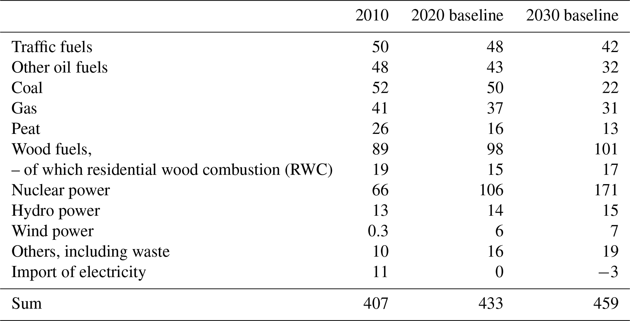
The assumptions about the future energy use, transport and other activities in Finland follow Finland's 2013 National Climate and Energy Strategy (Ministry of Employment and the Economy, 2013) and its baseline scenario that fulfills the agreed EU targets and specific national targets for a share of renewables and emission reductions in the sectors outside the Emission Trading Scheme. Table 2 shows the primary energy consumption by fuel in Finland in 2010 and 2030. The 2013 National Climate and Energy Strategy assumes the future prevalence of wood heating to remain at 2011 levels, which is estimated to lead to a decreased wood consumption, due to increasing energy efficiency in housing. The future emission projection was estimated with the FRES model which used the activity estimates from the 2013 National Climate and Energy Strategy (Table 2) as a basis.

Table 2 Primary energy consumption in Finland (TWh a⁻¹) (Ministry of Employment and the Economy, 2013).

2.2 Emission metrics

This work studies Finnish emissions with several climate metrics and focuses particularly on three of them: the AGWP (IPCC, 1990), AGTP (Shine et al., 2005) and ARTP (Shindell and Faluvegi, 2010). AGWP at time horizon H for emissions of pollutant i in emission season s from emission sector t is defined as

$$\begin{array}{}\text{(1)}& {\mathrm{AGWP}}_{i,s,t}\left(H\right)=\underset{\mathrm{0}}{\overset{H}{\int }}{\mathrm{RF}}_{i,s,t}\left(t\right)\mathrm{d}t,\end{array}$$

where RF is the time-varying radiative forcing given a unit mass pulse emission at time zero. Since two recent studies (Aamaas et al., 2016, 2017) have separated emissions during summer (May–October) and emissions during winter (November–April), we also make this separation when possible. AGTP is given as

$$\begin{array}{}\text{(2)}& {\mathrm{AGTP}}_{i,s,t}\left(H\right)=\underset{\mathrm{0}}{\overset{H}{\int }}{\mathrm{RF}}_{i,s,t}\left(t\right){\mathrm{IRF}}_T(H-t)\mathrm{d}t.\end{array}$$

IRF_T(H−t) is the temperature response, or impulse response function for temperature, at time H to a unit radiative forcing at time t. The ARTP is similar to AGTP but gives the temperature response in latitude bands m:

$$\begin{array}{ll}{\displaystyle }{\mathrm{ARTP}}_{i,m,s,t}\left(H\right)& {\displaystyle }=\sum _l\underset{\mathrm{0}}{\overset{H}{\int }}{\displaystyle \frac{F_{l,i,s,t}\left(t\right)}{E_{i,s,t}}}\times {\mathbf{RCS}}_{i,s,l,m}\\ \text{(3)}& {\displaystyle }& {\displaystyle }\times R_T\left(H-t\right)\mathrm{d}t,\end{array}$$

where $F_{l,i,s,t}\left(t\right)$ is the radiative forcing in latitude band l and ${\mathbf{RCS}}_{i,s,l,m}$ is the matrix of unitless regional response coefficients based on the ARTP concept (Collins et al., 2013). In Sand et al. (2016), RCS matrices differ for some of the different sectors; for example, BC emissions in the Nordic countries from the domestic sector have a sensitivity about 15 % higher than BC emissions from energy and industry. Aamaas et al. (2017) do not provide this information on a sector level, and we must therefore use the same RCS matrix for all emission sectors.

The ARTP method divides the world into four latitude bands: southern mid- to high latitudes (90–28^∘ S), the tropics (28^∘ S–28^∘ N), northern midlatitudes (28–60^∘ N) and the Arctic (60–90^∘ N). We will focus on the temperature response in the Arctic, as well as the global mean response.

Some of the studies separate the net response for a pollutant into various processes. For the aerosols, the radiative efficiencies often include the aerosol direct and first indirect (cloud-albedo) effect. In addition, BC deposition on snow and semi-direct effects may also be considered for BC. The ozone precursors build on the processes of a short-lived ozone effect, methane effect and methane-induced ozone effect, as well as the aerosol direct and first indirect effects.

All these emission metrics (AGWP, AGTP, ARTP) can be normalized to the corresponding effect of CO₂, where M is GWP, GTP, or RTP:

$$\begin{array}{}\text{(4)}& M_i\left(t\right)={\displaystyle \frac{{\mathrm{AM}}_i\left(t\right)}{{\mathrm{AM}}_{{\mathrm{CO}}_{\mathrm{2}}}\left(t\right)}}.\end{array}$$

For GWP, we have included an additional analysis with the newly suggested metric GWP^* (Allen et al., 2016, 2018). They argue for an alternative use of GWP to better compare CO₂ and SLCFs, which can be done by comparing the cumulative warming of CO₂ with the emission level change of SLCFs. For CO₂ and N₂O, we have calculated GWP^*(H) based on Eqs. (1) and (4), which leads to CO₂-equivalent emissions for pollutant i_L between time t₁ and t₂:

$$\begin{array}{}\text{(5)}& E_{{\mathrm{CO}}_{\mathrm{2}}\text{-}{\mathrm{eq}}^{\ast },i_L}=\sum _{t_{\mathrm{1}}}^{t_{\mathrm{2}}}{E}_{i_L}\times {\mathrm{GWP}}_{i_L}\left(H\right).\end{array}$$

For SLCFs, the CO₂-equivalent emissions are

$$\begin{array}{}\text{(6)}& E_{{\mathrm{CO}}_{\mathrm{2}}\text{-}{\mathrm{eq}}^{\ast },i_S}=\mathrm{\Delta }{E}_{i_S}\times {\mathrm{GWP}}_{i_S}\left(H\right)\times H.\end{array}$$

$\mathrm{\Delta }{E}_{i_S}$ is the change in emission level for SLCP i_S between time t₁ and t₂. We have compared emissions for the 2000–2030 period and with a time horizon of H=100 years.

The pollutants we include in our analysis (SO₂, NO_x, NH₃, NMVOC, BC, OC, CO, CO₂, CH₄ and N₂O) have very different atmospheric lifetimes and impact pathways. For the greenhouse gases (GHGs) (CO₂, CH₄ and N₂O), we use the climate metric parameterization in IPCC AR5 (Myhre et al., 2013), but with an upward revision of 14 % for CH₄ to account for the larger radiative forcing calculated by Etminan et al. (2016). The atmospheric decay of CO₂ is parameterized based on the Bern Carbon Cycle Model (Joos et al., 2013) as reported in Myhre et al. (2013). We assume that the relative temperature response pattern in the four latitude bands is the same for all the GHGs, and we base our calculations on the latitude pattern for CH₄ in Aamaas et al. (2017).

For all the other pollutants (SO₂, NO_x, NH₃, NMVOC, BC, OC and CO), we use several recent studies that are relevant for the emission location, Finland (Aamaas et al., 2016, 2017; Sand et al., 2016). We have examined how metric values from all those studies can be used for Finnish emissions and compared those, but we will mainly present combinations of the studies that we think combine the strengths of the different datasets. For a general and global view, we have used the GWP and GTP values from Aamaas et al. (2016). The rest of the paper utilizes ARTP values from Aamaas et al. (2017) to estimate temperature responses, with scaling from Sand et al. (2016) for temperature responses in the Arctic. Aamaas et al. (2017) is our starting point as this study has the full set of emissions and separates summer and winter emissions.

No studies have presented climate metric values specific to Finnish emissions. The default choice would be to use climate metric values based on global emissions, while we believe using smaller emission regions near or including Finland is more representative than applying the global average. The most relevant emission regions in the three selected studies are Europe (consisting of western Europe, eastern members of the European Union and Turkey, up to 66^∘ N) for Aamaas et al. (2016, 2017) and the Nordic countries for Sand et al. (2016). The Nordic countries is a smaller region and is geographically more representative of Finland than Europe is. Therefore, we have calculated ratios between metrics for the Nordic region vs. Europe in Sand et al. (2016) and used those ratios to scale the metric values from Aamaas et al. (2017) to better represent Finnish emissions. However, Sand et al. (2016) provided climate metric values only for the Arctic response, their set of pollutants was limited to BC, OC and SO₂, and for the ozone precursors they included only a combined response. To solve this we have used averages, such as taking a weighted average of the different emission sectors for each pollutant and assuming that NH₃ can be scaled by an average of BC, OC and SO₂. The scaling we have done for the Arctic responses is 2.22 for BC, 3.09 for BC deposition in snow, 2.32 for OC, 1.94 for SO₂, 2.16 for NH₃, and 1.00 for NO_x, CO and NMVOC. This scaling for the Arctic will also increase the global responses but will not affect the coefficients for the other temperature response bands.

For all the pollutants, the IRF for temperature comes from the Hadley Centre Coupled Model version 3 (HadCM3) (Boucher and Reddy, 2008). Hence, our temperature calculations are based on a climate sensitivity of 3.9 K warming for a doubling in CO₂ concentration.

Most emissions stay relatively constant throughout the year, while the changing seasons result in much larger emissions from the domestic sector in winter than in summer. We account for this seasonality for those metric datasets compatible with this; otherwise, annual emission and metric values are applied.

The global and regional temperature responses of Finnish emissions are estimated by convolving ARTP values with emissions. For an emission scenario E(t), the global temperature response is

$$\begin{array}{}\text{(7)}& \mathrm{\Delta }{T}_{i,s,t}\left(t\right)=\underset{\mathrm{0}}{\overset{t}{\int }}{E}_{i,s,t}\left(t^{\prime }\right)\times {\mathrm{AGTP}}_{i,s,t}\left(t-t^{\prime }\right)\mathrm{d}{t}^{\prime }\end{array}$$

based on AGTP values. Similarly, the temperature responses in latitude bands can be estimated by replacing AGTP with ARTP values. As mentioned, the ARTP method divides the world into four latitude bands, and thus the global temperature response can also be estimated by using the ARTPs and taking the area-weighted global mean based on the results for the latitude bands. As the forcing-response coefficients are different and the ARTP concept can better parameterize varying efficacies, the estimated global temperature response may vary depending on whether it is based on AGTPs or based on ARTPs.

Our climate impact dataset can be analyzed in many different dimensions, such as for different timescales, for different emission sectors, for different processes, or for pulse or scenario emissions. We show some examples. As we focus on near-term climate change and the global and regional temperature, most of the discussion in this paper utilizes ARTP for the mean warming in the first 25 years after a pulse emission, as recently proposed by Shindell et al. (2017). Mean ARTP (1–25 years) is the average temperature response over the time period, which differs from ARTP (25 years), being a snapshot at the time horizon of 25 years. It has similarities to the integrated global temperature change potential (iGTP) concept introduced by Peters et al. (2011). We want to point out that our choice of metric is not based on a thorough scientific analysis but rather is a subjective choice to study the near-term climate impacts and the importance of short-lived species in more detail. To balance the choice we compare it with some other known climate metrics.

3 Results

3.1 Emissions

Figure 1 shows the Finnish emissions and their trends from 2000 until 2030 for the studied pollutants. Emissions by sector for 2000, 2010 and 2030 can be found in Table S1 of the Supplement. Emission reductions are expected for practically all of the pollutants and greenhouse gases, especially between 2010 and 2030, but the magnitude differs between the species. Reductions of CO₂ and SO₂ take place to a large extent in the energy production sector following the reduction of energy consumption of fossil fuels, i.e., coal, oil and peat (Table 2).

CH₄ emissions have declined mostly due to developments in the waste sector. The amounts of methane recovered from landfills have increased during the study period following EU and national regulations. Methane emissions from landfills have also declined because there has been an increase in the use of municipal solid waste for energy instead of depositing it in landfill, a development that is expected to continue also until 2030. Another factor explaining the declining emissions by 2030 is the prohibition of the disposal of organic waste to landfills after 2016.

The transport sector is responsible for the decline in the emissions of CO, NO_x and VOC as well as the particle species, BC and OC. The modernization of vehicles and consequent introduction of stricter emission controls required by the European emission standards explain the decline in CO, NO_x and NMVOC emissions. The standards do not directly regulate BC or OC emissions, but since they are the main constituents of the regulated particulate emissions, reductions in emissions of BC and OC are expected, especially after the introduction of the diesel particulate filters for on-road light-duty vehicles from 2010 onwards. The heating stoves and boilers in the residential sector will remain significant emitters of several pollutants, since the regulation following the European Union Ecodesign directive will not have a major impact by 2030, due to the relatively long lifetime of Finnish heaters (Savolahti et al., 2016).

NH₃ and N₂O emissions remain relatively stable throughout the study period, since either much of the emission reductions has already taken place before the study period or no major changes are expected in the main emission sectors (agriculture for NH₃).

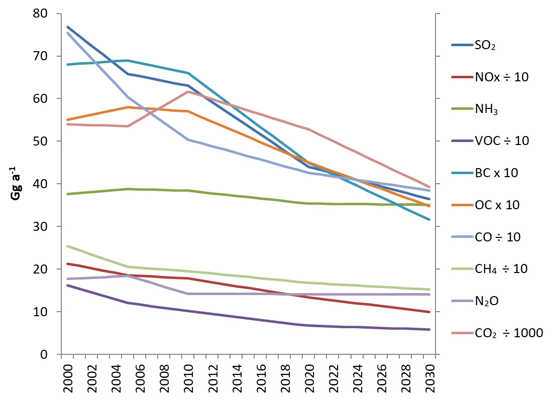
Figure 1 Finnish emissions (Gg a⁻¹) of air pollutants and greenhouse gases in the period 2000 to 2030 in the baseline scenario. Emissions by sector for 2000, 2010 and 2030 can be found in Table S1 of the Supplement.

3.2 Climate impact of Finnish emissions

Figure 2 shows pulses of 2010 emissions weighted with the global metrics (GWP and GTP) to CO₂ equivalents using 10-, 20-, 50- and 100-year perspectives. Aamaas et al. (2013) studied global emissions with these metrics, while we focus in detail on Finnish emissions. In addition, we show the emission metric mean GTP (1–25 years), which gives the SLCFs a relatively large weight, similar to GTP (10 years) for the aerosols and in between GTP (10 years) and GTP (20 years) for CH₄. In Fig. 2 the emissions are considered as a pulse and the figure does not take into account any emissions after 2010. Figure 2 demonstrates that the SLCFs have a larger relative importance with the metrics for shorter time horizons. However, in all cases CO₂ still is the most important species. With the emission metric with the 10-year horizon (GTP10) the warming SLCFs comprise more than two-thirds of the warming effect of CO₂, but overall the net impact of all short-lived species is about 30 % of CO₂, due to the partly counteracting cooling effect of NH₃, SO₂, NO_x and OC. The relative importance of the SLCFs decreases with time, especially with GTP, as expected, and the relative effect is lowest with the temperature change metric with 100-year time horizon (GTP100), being about 6 % of CO₂. Among the non-CO₂ emissions, the relative impact of N₂O increases with increasing time horizon due to the much longer atmospheric lifetime than for the other pollutants.

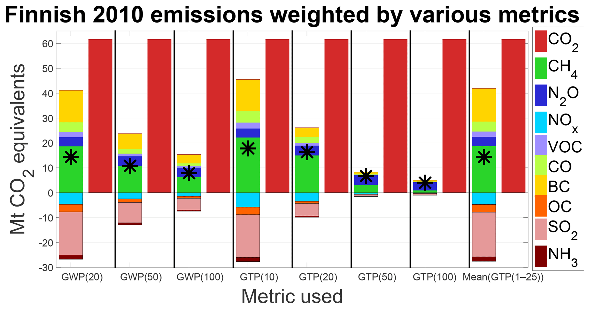
Figure 2 Finnish 2010 emission (Mt CO₂ equivalents) as a pulse emission weighted by various global metrics. CO₂ is separated out and the net impact of the non-CO₂ is given by the star.

An alternative to comparing emissions pulses with GWPs and GTPs is to consider the impact over a particular emission time period with GWP^* (Allen et al., 2016, 2018). Figure 3 presents a GWP^*-based analysis of Finnish emissions. As we have looked at emissions for the period 2000–2030, the CO₂-equivalent emissions given in Fig. 3 are not directly comparable to those based on pulses in Fig. 2. We find that changes in global temperature in this period are mostly governed by the cumulative emissions of CO₂. The emissions of multiple SLCFs decline in this period (Fig. 1), resulting in a net cooling and counteracting 4 % of the warming by CO₂ and N₂O. If emissions of all SLCFs were hypothetically reduced to zero in this period, this emission change could counteract the warming by CO₂ and N₂O by about one-third. Similarly, as for GWPs and GTPs (Fig. 2), we find that emission of CO₂ has the largest impact of all pollutants.

Figure 3 The CO₂-equivalent emissions for the period 2000–2030 given the alternative metric GWP^*(100). The net impact of SLCFs (left) and CO₂ and N₂O (right) is given by the star.

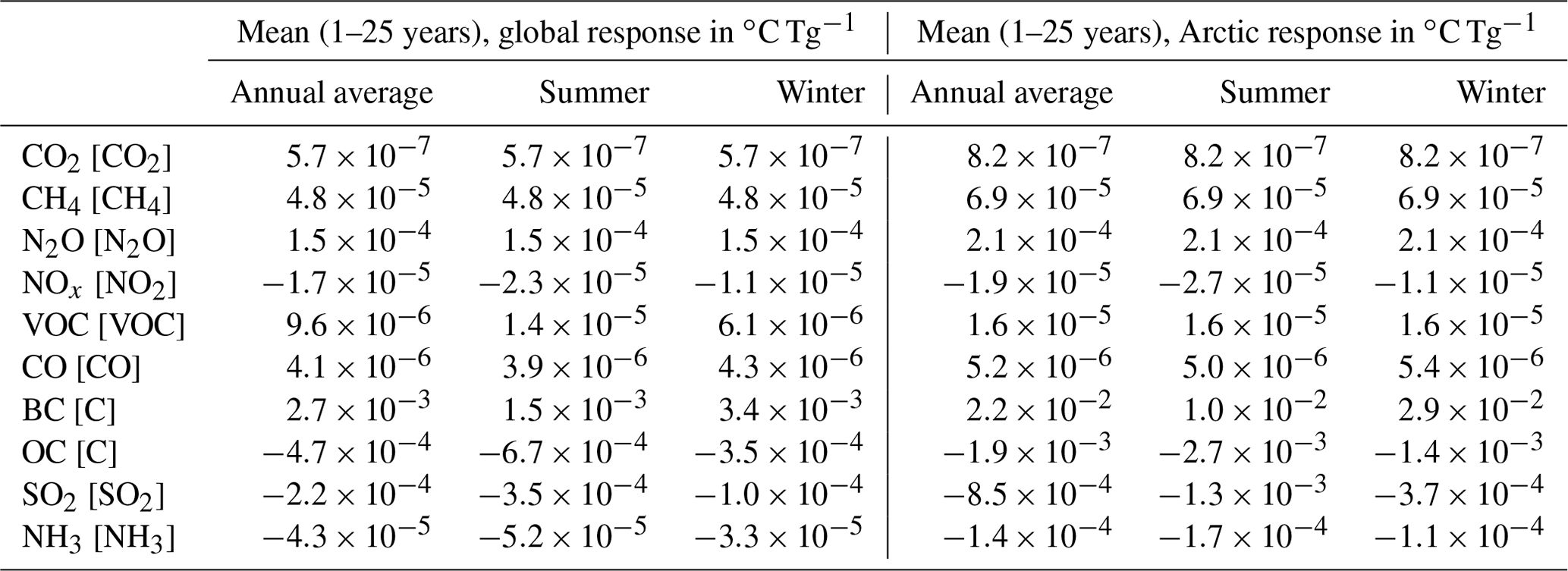
As we focus on near-term climate change and the global and regional temperature, the remaining paper utilizes ARTP with a time horizon of mean GTP (1–25 years), as proposed by Shindell et al. (2017). ARTP values are applied, following the argumentation by Aamaas et al. (2017) that ARTPs may give a better estimate of the global impact than AGTPs since they account for varying efficacies with latitude to a larger degree. The ARTP (1–25 years) used in this study is presented in Table 3. GWP^* could also be a basis to estimate global temperature changes, but that would not give us regional temperature changes.

Table 3 The climate metric values (^∘C Tg⁻¹) used in this study. Mean ARTP (1–25 years) values for SLCF and GHG emissions. The Arctic response for the GHGs is based on the latitudinal pattern for CH₄. The annual average is based on emissions in 2010. Normalized values (CO₂ equivalents) are shown in Table S2.

3.2.1 Climate impacts by emission sector

This section discusses the global temperature response of the emissions by pollutant and emission sector based on weighted ARTP values (Aamaas et al., 2017). The general findings described in the following paragraphs would be similar with AGTPs, and similar figures based on the AGTP values (Aamaas et al., 2016) can be found in Fig. S1 of the Supplement for comparison. Figure 4a, b and c show the warming due to emissions in 2000, in 2010 and in 2030, following the baseline projection, respectively. The sum of all sectors is given in Fig. 4d. The pollutant mix varies for the different sectors. CO₂ is the most important pollutant for combustion in ENE IND and TRA RD, while methane is most important for the WST and AGR sectors. BC emissions cause more than two-thirds of the warming, increasing over time in DOM and causing a significant share of the warming in TRA RD as well as TRA OT sources. The rest of the warming effect for these sectors is due to CO₂ emissions from fossil fuels, especially diesel and light fuel oil. Wood is an important fuel in the domestic sector, and since this study considers wood fuel as CO₂ neutral, the CO₂ warming effect is not as pronounced as, for example, in the on-road transport sector. Organic carbon was the most important cooling agent in domestic and the transport sectors, as fuelwood does not contain much sulfur. Furthermore, it was phased out from liquid fuels in the transport sector. Overall, SO₂ is the major cooling pollutant mainly due to emissions from ENE IND and PROC. Agriculture is an important source of ammonia (NH₃), which has a cooling effect (Figs. 4a–c and 5a) via its participation in the formation of cooling atmospheric aerosols like ammonium sulfates and nitrates.

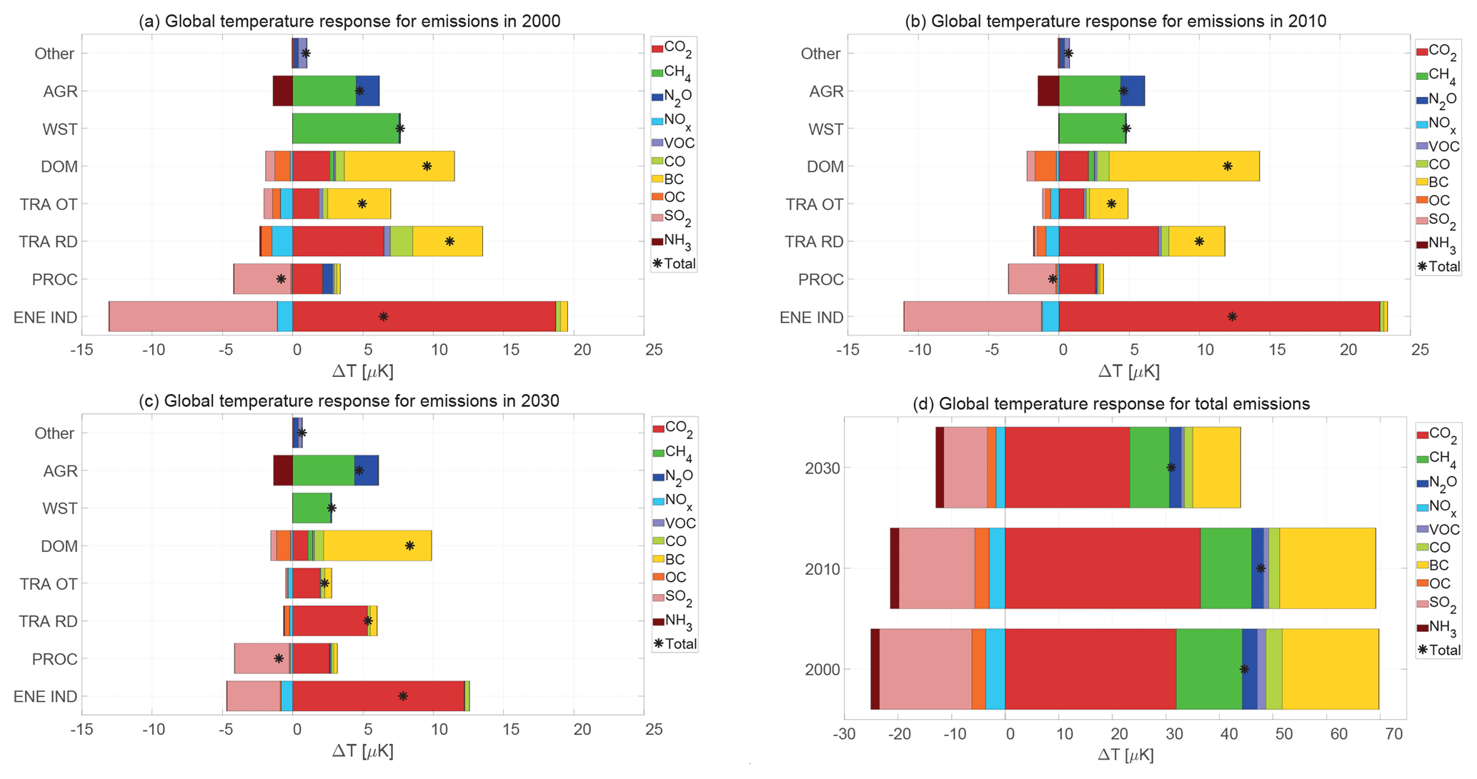
Figure 4 The temperature response (µK) due to emissions in 2000 (a), 2010 (b) and 2030 (c) from energy and industry sectors (ENE IND), industrial processes (PROC), road transport (TRA RD), off-road transport and machinery (TRA OT), domestic (DOM), waste (WST), agriculture (AGR) and other (OTHER). The sum of all sectors is shown in (d). The climate metric applied is the global mean ARTP (1–25 years) for pulse emissions.

The year 2000 was relatively warm and 2010 relatively cold in Finland, which is reflected by the higher use of coal, peat and wood fuels in 2010 and consequently also by the higher emissions of some species. From 2000 to 2010, CO₂ emissions from ENE IND increased by 22 % and BC emissions from DOM by 37 %. However, because of additional mitigation measures following legislation, CH₄ emissions from the WST decreased by 38 %. Also, despite the higher fuel use, improved flue gas cleaning measures caused SO₂ emissions in ENE IND to decrease by 18 %. On the other hand, the reduction of SO₂ increased the warming effect of the ENE IND sector in 2010 compared to 2000. The increasing SLCF emissions in the DOM sector, particularly black carbon, led to additional net warming despite the fact that the organic carbon emissions offset about a fifth of the black carbon effect in both years. The decreasing trend for the use of heating oil in the domestic sector has reduced CO₂ emissions between 2000 and 2010. Emissions from the PROC sector are relatively neutral in terms of their climate effect. In general, taking into account all sectors, the emission changes between 2000 and 2010 in Finland have led to net warming (increase by 7 %), mostly due to the increase in CO₂ emissions (warming) and the decrease in SO₂ emissions (warming) from the ENE IND sector, which offset the reduction of CH₄ emissions (cooling) in the WST sector.

The baseline projection will lead to an emission reduction of all pollutants between 2010 and 2030, from a reduction of BC greater than 50 % to a small reduction of N₂O (Fig. 1 and Table S1). Because of climate policies, CO₂ emissions are reduced following the declining use of fossil fuels (Table 2, Fig. 4b, c and d). The SO₂ emissions continue their decline between 2010 and 2030, particularly in the ENE IND sector, which leads to additional warming but only partly offsets the reduced CO₂ (Fig. 4b, c and d). In the TRA RD and TRA OT sectors, the warming effect from the SLCFs, in particular, declines because the new vehicles, in order to comply with the European emission legislation, are equipped with efficient emission reduction technologies (Fig. 4b and c). The amount of domestic wood combustion is expected to decrease in the baseline due to improved energy efficiency in housing, which is the main reason for the reduced SLCF emissions in the sector (Fig. 4b and c). However, when interpreting these results, it is important to note that the prevalence of domestic wood combustion has increased during the 2000s and the future wood use in households is challenging to predict. Therefore, the emissions from the domestic sector should be considered uncertain. This is demonstrated in a sensitivity analysis of future particle emissions from the domestic sector presented by Savolahti et al. (2016). Also, the methane emissions in the WST sector continue their decline (Fig. 4b and c). As a consequence of the emission changes, the net temperature impact of 2030 emissions is 35 % lower compared to the 2010 emissions (Fig. 4d). Practically all sectors except AGR contribute to the reduced warming (Fig. 4b, c).

3.2.2 Cumulative temperature development 2000–2030

While most of our study focuses on emission pulses, in this section we will discuss global temperature responses given a convolution of a Finnish emission scenario and ARTP values. The cumulative global temperature impact by pollutants and sectors for Finnish emission from 2000 to 2030 is shown in Fig. 5, based on ARTPs in Aamaas et al. (2017) and Sand et al. (2016). Similar figures based on AGTP values (Aamaas et al., 2016) are given in Fig. S2 of the Supplement. Figure 5 demonstrates why emission reductions of CO₂ and other long-lived greenhouse gases are key for limiting the long-term surface temperature increase. As more years are added, the relative importance of CO₂ increases, since a large portion of it stays in the atmosphere for hundreds of years. This relative importance over time also occurs in the case of N₂O. The air pollutants become of less relative significance with time, which is mostly because of those pollutants being quickly removed from the atmosphere, but also because of the reduced emissions levels in the later period. Almost all sectors have a net warming temperature response, with the exception of cooling from the ENE IND sector for more than the first 10 years and a slight cooling from the PROC sector until 2030 (Fig. 5b). Cooling from mainly SO₂ emissions offsets the warming impact of CO₂ from those sectors. Over time, ENE IND becomes the most influential sector, being the single largest contributor of CO₂. BC is the most significant warming pollutant in the domestic sector, and in the agriculture and waste sectors, it is CH₄.

Figure 5 The global temperature development (mK) of Finnish emissions for the period 2000–2030. Temperature is given by pollutants in (a) and by sectors in (b). The global temperatures are estimated as a convolution of ARTP values and an emission scenario.

3.2.3 Seasonal temperature response from Finnish emissions

The estimated temperature response of Finnish emissions varies between the seasons. In Fig. 6, we compare Finnish SLCF emissions for the year 2010 during summer (May–October) and winter (November–April). A decomposition into different atmospheric forcing processes is also included. When we do not consider CO₂, N₂O and CH₄, the pollutants give a net cooling for emissions in summer and a net warming of equal size for emissions in winter. The main driver for this is larger BC emissions in winter combined with a much stronger response from the snow albedo effect. The reason is that more than 70 % of the annual emissions in the domestic sector occur in winter. Another important difference is the much stronger cooling by SO₂ in summer. Some pollutants have both warming and cooling processes, such as BC and NO_x. The same process can be warming for one pollutant and cooling for another; for example NO_x emissions remove CH₄ from the atmosphere (cooling), while VOC and CO emissions add CH₄ (warming). Changes in the methane concentration will also influence ozone, giving rise to the methane-induced ozone effect and reinforcing the methane effect.

For 1 t of BC emission with the ARTP metric, the wintertime impact is higher by more than 120 % than the summertime impact. Almost 80 % of the net impact for winter emission comes for BC deposition on snow. The annual impact of winter emissions of BC is almost 80 % with the ARTPs. From a mitigation perspective, these estimates indicate that attention should be placed on reducing winter emissions of BC.

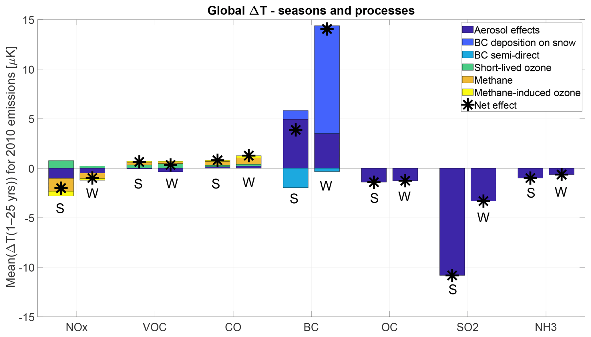
Figure 6 The global temperature response (µK) of Finnish emissions in 2010 by applying the mean temperature 1–25 years after the pulse emission. This figure compares emissions occurring in summer (S) vs. winter (W) by applying ARTP values (Aamaas et al., 2017; Sand et al., 2016). The responses are divided into six different processes.

3.2.4 Arctic temperature response from Finnish emissions

The seasonal differences for the SLCFs are also clearly seen in the Arctic temperature response (Fig. 7). Finland is closely situated to the Arctic as practically the whole country is north of 60^∘ N and a significant area lies north of the Arctic Circle. Figure 7 shows the Arctic (between 60 to 90^∘ N) temperature response based on the ARTP metrics from Aamaas et al. (2017) and Sand et al. (2016). As a general observation, the temperature responses are larger in the Arctic (Fig. 7) than globally (Fig. 6). The trends are similar, with net cooling of summer emissions and net warming of winter emissions. The Arctic warming in winter is up to about 3 times larger than the cooling in summer, mostly due to the outsized impact of wintertime emissions of BC. However, during summer, the cooling by SO₂ emissions outweighs the warming by BC emissions.

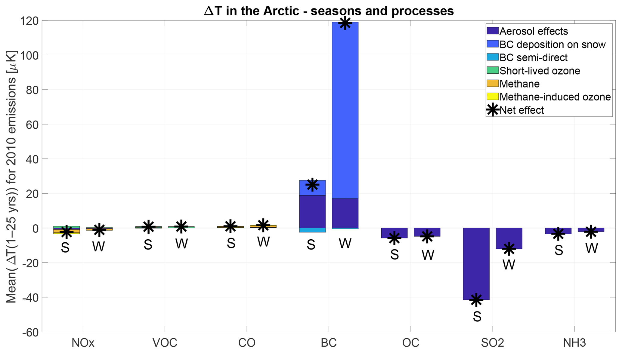
Figure 7 The temperature response (µK) in the Arctic of Finnish emissions in 2010, by applying the mean temperature 1–25 years after the pulse emission. This figure compares emissions occurring in summer (S) vs. winter (W) by applying ARTP values (Aamaas et al., 2017; Sand et al., 2016).

Figure 8 compares global and Arctic temperature responses to Finnish emissions of all pollutants considered in this study, using the Aamaas et al. (2017) approach. It demonstrates that the temperature response in the Arctic is typically stronger than the global average. If we apply the ARTP methodology for GHGs, the response in the Arctic is up to 50 % larger than the global average due to stronger local feedback processes in the Arctic (Boer and Yu, 2003). The ozone precursors have similar or weaker efficacies in the Arctic compared with the GHGs. However, the aerosols and sulfur emissions stand out with the largest differences (Fig. 8). By applying ARTP values from Aamaas et al. (2017) with scaling from Sand et al. (2016), we find that Finnish emissions of SO₂ and OC have a 300 % stronger efficacy in the Arctic than the global average, and this is even higher for BC with 700 %. A limitation of this method is that the scaling from Sand et al. (2016) is only applicable for the Arctic temperature response, which adds some uncertainties to the Arctic vs. global ratios. For BC, this amplification in the Arctic is even stronger for emissions occurring in winter. Hence, the results indicate that mitigation of Finnish BC emissions is especially beneficial for limiting Arctic warming.

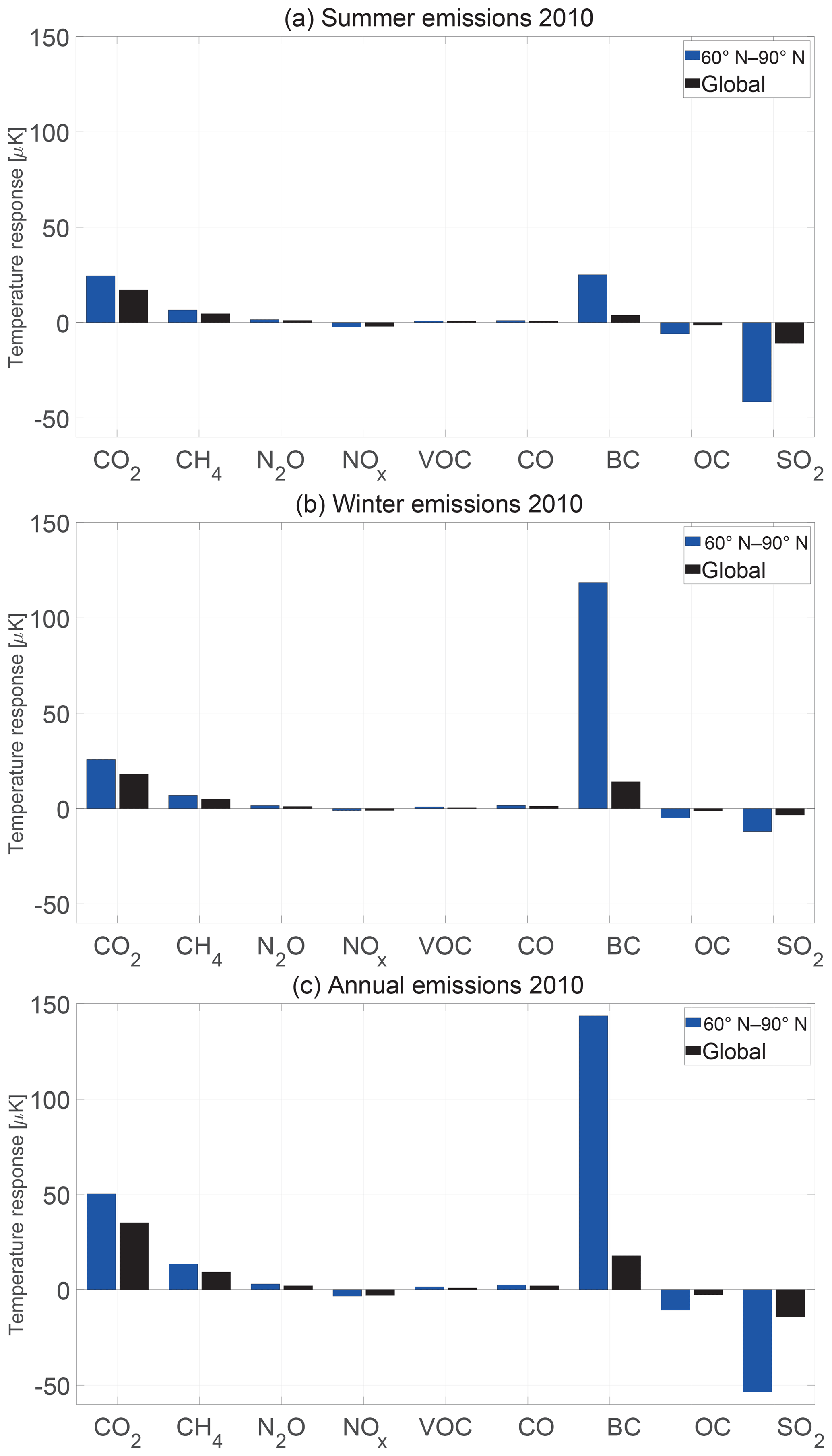
Figure 8 Global and Arctic (60–90^∘ N) temperature responses (µK) to Finnish emissions based on ARTP values in Aamaas et al. (2017) and Sand et al. (2016). As for most of the figures, the temperature response is the mean response 1 to 25 years after a pulse emission.

4 Discussion

The first objective in our study was to produce an integrated multi-pollutant emission dataset for Finland for 2000 to 2030. We were able to achieve this aim, but it required the use of several data sources and studies that are not necessarily maintained on a regular basis. Future efforts should seek to maintain the integrated multi-pollutant database developed for this work. This would require an integrated modeling environment, for example the FRES, and would require further work to fill in the gaps for the missing sectors and pollutants via developing relevant activity and emission factor databases into the FRES framework.

Our second set of objectives for this study aimed to compare different climate metrics and to assess their suitability for calculating the climate impact of a multi-pollutant emission set. Several air pollutants and greenhouse gases have detrimental impacts on global and regional climate, human health and wellbeing, as well as crop yields (Shindell et al., 2012). Since the magnitudes and pathways of the effects differ between the constituents, integrated modeling is needed to understand the consequences and form the basis for robust climate and air quality policies. This paper applied and compared various climate metrics to study the approximate integrated climate impact of Finnish air pollutant and greenhouse gas emissions globally and in the Arctic area. The results demonstrated that the relative impacts and importance of individual species as well as sectors can differ significantly between the studied temporal-response scales, emission seasons as well as geographical scales for both emission sources and temperature responses. The warming or cooling impact of SLCFs is especially sensitive to the studied timescale, with shorter time spans showing greater importance compared with GHGs.

Finnish emissions and their climate responses are relatively small; therefore, it is challenging to use climate models to study the climate effect of national policies and to analyze the role of each pollutant and sector. This study demonstrated a method to overcome this challenge by utilizing emission metrics. All studied metrics provided interesting insights into the impacts of Finnish emissions and which aspects could be emphasized when formulating mitigation strategies. We found that the ARTP-based metrics, in particular, provided useful information. We preferred to use ARTP approaches to assess the impacts of Finnish emissions on both the global and Arctic climates because they include the regional or latitudinal dimension of emission impacts in more detail. We also chose to use the mean 1–25-year time frame, since for the time being there are no established climate metrics for air pollutants, and this approach was recently suggested by Shindell et al. (2017) to be used in connection with SLCFs. This is a subjective choice to study the near-term climate impacts and the importance of short-lived species in more detail. To our knowledge, we are the first to present metric values with mean ARTP (1–25 years) and among the first to use the GWP^*.

The use of ARTPs to study the impacts of Finnish emissions is useful for designing national emission mitigation strategies also from a regional perspective. Finland is an Arctic country and a member of the Arctic Council, which is why there is high interest in understanding the Arctic impacts.

The third set of objectives aimed to estimate the climate impact of Finnish air pollutants and greenhouse gases utilizing the selected metrics. Our analysis across climate metrics, time horizons, pollutants and Finnish emission pathways demonstrated that carbon dioxide emissions have the largest climate response also in the near term (10 to 20 years), and their relative importance increases the longer the time span gets. Hence, mitigation of carbon dioxide is crucial for reducing the climate impact of Finnish emissions. In the near or medium term (i.e., 25-year perspective), methane and black carbon, in particular, have relatively significant warming impacts in addition to those of carbon dioxide. SO₂, on the other hand, is an important precursor to light-reflecting sulfate aerosol, thus having a cooling impact and offsetting part of the warming impact of the other species.

Concerning Finnish emissions, the combustion in energy production and industry has the largest global temperature impact over the medium and long term due to significant carbon dioxide emissions, while sulfur dioxide emissions induce a shorter-term cooling. Transport has the second biggest warming impact, and although that is expected to decrease notably by 2030 due to stricter control on particulate and black carbon emissions, it will remain a major source of carbon dioxide. Emissions from domestic and agriculture sectors also have a considerable warming impact, and they will remain as such, due to the relatively large respective emissions of black carbon and methane from the combustion of solid fuels, especially wood.

For all of the species the temperature response of Finnish emissions is generally stronger in the Arctic than globally but most significantly so in the case of black carbon and sulfur dioxide. Results obtained with the ARTP metric indicated that mitigation of wintertime black carbon emissions is especially important for reducing the temperature increase in the Arctic. Emissions of sulfur dioxide are expected to continue decreasing, and this has many benefits (Ekholm et al., 2014). However, they will offset some of the climate benefits of the reduced carbon dioxide emissions, and this should be taken into consideration in climate assessments.

The fourth major objective of this study was to recommend a set of global and regional climate metrics to be used in connection with Finnish SLCF emissions. As a preparation for writing this paper we compared several climate metrics to be used in connection with Finnish SLCF emissions. We ended up relying on those presented in Aamaas et al. (2017), which to our understanding, is currently the most complete set of climate metrics available for assessing the global and Arctic temperature responses of European emissions. However, we have scaled those values with ratios from Sand et al. (2016) for the Arctic temperature response because that study provided ARTPs for Nordic emissions, which are more representative of the Finnish case. For the GHGs, we argue for the application of the metric parameterization from IPCC AR5 (Myhre et al., 2013) but with an upward revision for CH₄ (Etminan et al., 2016). The coefficients for mean ARTP (1–25 years) (see also Shindell et al., 2017) in Table 3 were used for assessing different mitigation pathways in a 25-year time span. This time window is relevant for policies that focus on reducing global or Arctic warming in the near or medium term, from today and until 2040 or 2050. Corresponding mean RTP (1–25 years) values are shown in Table S2.

The assessed temperature impact of an emission dataset depends on the set of metrics available, as well as the applied metric setup, which bring uncertainties to the results. As there is no consensus on one individual set of metrics, especially in the case of air pollutants, the results will differ between different studies. This work estimated the global and regional temperature impacts of Finnish emissions based on methodologies in three recent papers (Sand et al., 2016; Aamaas et al., 2016, 2017). As all of these studies utilize partly the same radiative forcing datasets and partly similar general circulation models and chemistry transport models, we welcome other studies to complement the basis of our findings. Future work should continue to explore uncertainties and provide improved metrics.

Since the atmospheric lifetime of SLCFs is relatively short, their climate impact is more dependent on the emission region than with GHGs. Using Europe and the Nordic region as proxies for the emission region, as in this study, gives us a more representative picture of the Finnish case than the global average would give. Further development of the metrics should use more precisely the geographical location of Finland as the emission region in order to provide more precise temperature estimates for the Finnish emissions. The snow albedo effect of BC is expected to be much larger for the northernmost emissions, as indicated by a study on Norway by Hodnebrog et al. (2014). Future work should also focus on providing metrics for potentially missing species that could be important, for example dust aerosol.

Scientific literature has demonstrated that the climate impact of biomass combustion may depend on the timescale and forestry practices (i.e., Cherubini et al., 2011; Repo et al., 2012, 2015), which have not been a focus of this study. Since the use of biomass for energy is important in Finland and will likely remain so in the coming decades, future studies could utilize metrics to study its climate impacts. This study has mostly focused on surface temperature metrics; however, other interesting impacts could be studied using the metric approach. For example Shine et al. (2015) has recently presented a new metric named the global precipitation change potential (GPP), which is designed to gauge the effect of emissions on the global water cycle.

The understanding of the impact pathways of different pollutants has improved in recent years, which has led to further revisions of the climate impact estimates. Such developments are expected to continue. The metric studies, however, are often based on earlier radiative forcing studies, and there is a time lag between new scientific understanding and this being reflected in the climate metrics. This study has utilized the latest metric studies, but there is already literature available, for instance on BC, indicating that the temperature response may be smaller than demonstrated by the metrics used in this work (e.g., Stjern et al., 2017). As the understanding of the climate system improves, the estimates we give here for Finland should be revisited.

5 Conclusions

All studied metrics provided interesting insights into the impacts of Finnish emissions and which aspects could be emphasized when formulating mitigation strategies. We found that particularly the ARTP-based metrics provided useful information, although one should not rule out the significance of the other temperature and radiative-forcing-based metrics due to their relevance in connection with climate change mitigation work of the UNFCCC and IPCC. In the future, other climate impact metrics should also be explored and utilized. To enable such policy analyses an integrated multi-pollutant emission and metrics database, similar to the one used in this work, should be maintained.

Our analysis across climate metrics, time horizons, pollutants and Finnish emission pathways demonstrated that carbon dioxide emissions have the largest climate response also in the near-term, 10- to 20-year time perspective, and its relative importance increases the longer the time span gets. Hence, mitigation of carbon dioxide is crucial for reducing the climate impact of Finnish emissions. In the near or medium term (i.e., 25-year perspective), methane and black carbon, in particular, have relatively significant warming impacts additional to those of carbon dioxide.

For all of the species the temperature response of Finnish emissions is generally stronger in the Arctic than globally, but most significantly so in the case of black carbon and sulfur dioxide. The wintertime emissions, in particular, are net warming, and even more so in the Arctic, mostly due to black carbon. The snow albedo effect of the Finnish BC emissions is found to be large, and this phenomenon should be adequately included in the analyses. Since the atmospheric lifetime of SLCFs is relatively short, their climate impact is more dependent on the emission region than with GHGs. Using the Finnish case, our study demonstrated that future studies and further development of the metrics should use precisely the geographical location as the emission region in order to provide more precise temperature estimates.