the Creative Commons Attribution 4.0 License.
the Creative Commons Attribution 4.0 License.
 | 03 Jan 2019
Thermal structure of the mesopause region during the WADIS-2 rocket campaign
Boris Strelnikov
Timo P. Viehl
Josef Höffner
Pierre-Dominique Pautet
Michael J. Taylor
Yucheng Zhao
Franz-Josef Lübken
This paper presents simultaneous temperature measurements by three independent instruments during the WADIS-2 rocket campaign in northern Norway (69∘ N, 14∘ E) on 5 March 2015. Vertical profiles were measured in situ with the CONE instrument. Continuous mobile IAP Fe lidar (Fe lidar) measurements during a period of 24 h, as well as horizontally resolved temperature maps by the Utah State University (USU) Advanced Mesospheric Temperature Mapper (AMTM) in the mesopause region, are analysed. Vertical and horizontal temperature profiles by all three instruments are in good agreement. A harmonic analysis of the Fe lidar measurements shows the presence of waves with periods of 24, 12, 8, and 6 h. Strong waves with amplitudes of up to 10 K at 8 and 6 h are found. The 24 and 12 h components play only a minor role during these observations. In contrast only a few short periodic gravity waves are found. Horizontally resolved temperatures measured with the AMTM in the hydroxyl (OH) layer are used to connect the vertical temperature profiles. In the field of view of 200 km×160 km only small deviations from the horizontal mean of the order of 5 K are found. Therefore only weak gravity wave signatures occurred. This suggests horizontal structures of more than 200 km. A comparison of Fe lidar, rocket-borne measurements, and AMTM temperatures indicates an OH centroid altitude of about 85 km.
- Article
(7361 KB) - Full-text XML
- BibTeX
- EndNote


The MLT (mesosphere and lower thermosphere) region is one of the key regions for the interaction of planetary waves, tides, and gravity waves. Thermal tides are typically excited by solar heating of water vapour in the troposphere, ozone in the stratosphere and mesopause region, and oxygen above 90 km altitude. They can also be excited in the troposphere by latent-heat release due to deep convection (Chapman and Lindzen, 1970; Forbes, 1984; Hagan and Forbes, 2002). Due to the excitation processes, tides have periods of the solar day (24 h) and its harmonics (12, 8 h, …). Gravity waves are mostly generated in the troposphere and lower stratosphere by the flow above orographic structures, convective instabilities, wind shears, jet streams, or wave–wave interactions (Fritts and Alexander, 2003). Their propagation depends on the background wind field and its modulation by tides and planetary waves (Eckermann and Marks, 1996; Senf and Achatz, 2011). The different atmospheric layers are coupled by the transport of momentum and energy on a wide range of scales due to the propagation and interaction of these waves. Gravity waves and tides are therefore a key driving mechanism for atmospheric processes and play an important role in their understanding.
Our knowledge of properties of the MLT region is still very limited. The main reason for this lack of knowledge is the difficulty of experimental research at this altitude. Detailed and continuous measurements are still rare (Smith, 2012). In recent decades different techniques have been developed to investigate the MLT region. While satellites provide a global overview of the atmosphere, it is not possible to investigate variability on short timescales since they typically need several weeks to cover 24 h of local time. In situ observations with sounding rockets are local measurements with high resolution and precision but can only be realised sporadically. Remote sensing methods typically rely on specific phenomena which appear in the mesopause region, e.g. meteors evaporating at these altitudes. This creates layers of metallic atoms such as iron (Fe) which can be probed by resonance lidars to derive temperatures. Furthermore, the specific chemistry of the mesopause region creates a persistent hydroxyl (OH) layer. The airglow resulting from excited OH molecules can be detected from ground-based imagers to derive temperatures and horizontally resolved wave information.
This paper shows results from experimental investigation of temperatures in the mesopause region in the frame of the WADIS-2 sounding rocket campaign, which make it possible to study the MLT region with high temporal and spatial resolution. The name WADIS stands for “Wave propagation and dissipation in the middle atmosphere: Energy budget and distribution of trace constituents”. The main goal of the campaign, led by the Leibniz-Institute of Atmospheric Physics (IAP), was to study propagation of gravity waves from their sources in the troposphere to their level of dissipation in the MLT and quantification of their contribution to the energy budget of the upper atmosphere. For an overview of the WADIS project and its main mission the reader is referred to Strelnikov et al. (2017). In Sect. 2 three instruments providing MLT temperature observations with some important parameters are described. The observations and their analysis are described in Sect. 3. Finally, the results are discussed in Sect. 4, and a short summary is given in Sect. 5.
Three instruments provided direct and indirect temperature observations in the MLT region during the WADIS-2 campaign. The CONE instrument on board the WADIS-2 rocket, the mobile IAP Fe lidar, and the Utah State University Advanced Mesospheric Temperature Mapper (AMTM) are analysed in this study. These instruments are briefly introduced in the following.
The WADIS-2 payload was equipped with two identical CONE instruments (COmbined sensor for Neutrals and Electrons) on the front and rear deck of the payload. They measure turbulence, neutral air temperature and density, and electron density with very high spatial resolution of the order of centimetres (Giebeler et al., 1993; Strelnikov et al., 2013). Data acquisition is performed independently for each sensor. As the rocket probes the upper atmosphere, the centre of mass of the payload follows a ballistic curve but the orientation remains roughly upright. This means that the same ends of the payload are always facing upwards and downwards. The data of the respective CONE sensors pointing in the direction of the flight (front bay for the upleg, rear bay for the downleg) are analysed in this study. More details on the CONE instrument and the complete payload instrumentation can be found in Giebeler et al. (1993) and in Strelnikov et al. (2013, 2017).
Two further instruments providing ground-based observations of temperatures in the mesopause region are located at the ALOMAR observatory (Arctic Lidar Observatory for Middle Atmosphere Research), at a distance of approximately 2 km to the south of the WADIS-2 rocket launch site at the Andøya Space Center.
The mobile IAP Fe lidar (Fe lidar) has been operating at the ALOMAR observatory since summer 2014. It determines mesospheric temperatures and Fe densities by probing the Doppler-broadened Fe resonance line at 386 nm with a frequency-doubled alexandrite ring laser. The system can measure during night and day. Observations in full daylight are nearly free of solar background radiation. The receiving telescope is pointed vertically. The altitude range of accurate resonance lidar temperature measurements is limited to about 75 to 100 km due to the extent of the meteoric Fe layer (Lautenbach and Höffner, 2004; Viehl et al., 2016). Further information about the instrument has been published by Lautenbach and Höffner (2004) and Höffner and Lautenbach (2009), for example.
The Utah State University (USU) Advanced Mesospheric Temperature Mapper (AMTM) (Pautet et al., 2014) was installed at the ALOMAR observatory in 2010 and measures OH (3,1) rotational temperatures at the altitude of the OH layer. An altitude range of 82 to 90 km is typical for the OH centroid height (Baker and Stair, 1988; von Zahn et al., 1987). The AMTM can observe temperatures with high temporal and spatial (horizontal) resolution during the night even in presence of auroras. During the day, the solar background rises above the OH emission, which prevents further observations. An OH intensity and temperature map with a resolution of 320 pixels×256 pixels (0.6 km×0.6 km per pixel) is taken from the OH layer every 30 s. This corresponds to an overall area of 200 km×160 km centred at the observation site (ALOMAR). In Pautet et al. (2014) more information on the instrument and its development are given.
The horizontal arrangement of the measurement volumes at the OH layer altitude is shown in Fig. 1. The features in the vertical profiles can be connected by the horizontally resolved structures in the AMTM temperature maps and identify them as the same or different phenomena. As illustrated in Fig. 1, the WADIS-2 rocket was launched in an approximately north-western direction. The marks labelled “rocket upleg” and “rocket downleg” indicate the positions at which the rocket passed through the OH layer during the up- and the downward flight paths, respectively. The “Fe lidar” mark defines the location of Fe lidar measurements at the ALOMAR observatory, where the AMTM is also located. The crosses on the map mark only the location, not the size of the CONE and the lidar measurement volumes. Their horizontal extent is of the order of several centimetres for the CONE sensors and several tens of metres for the Fe lidar.
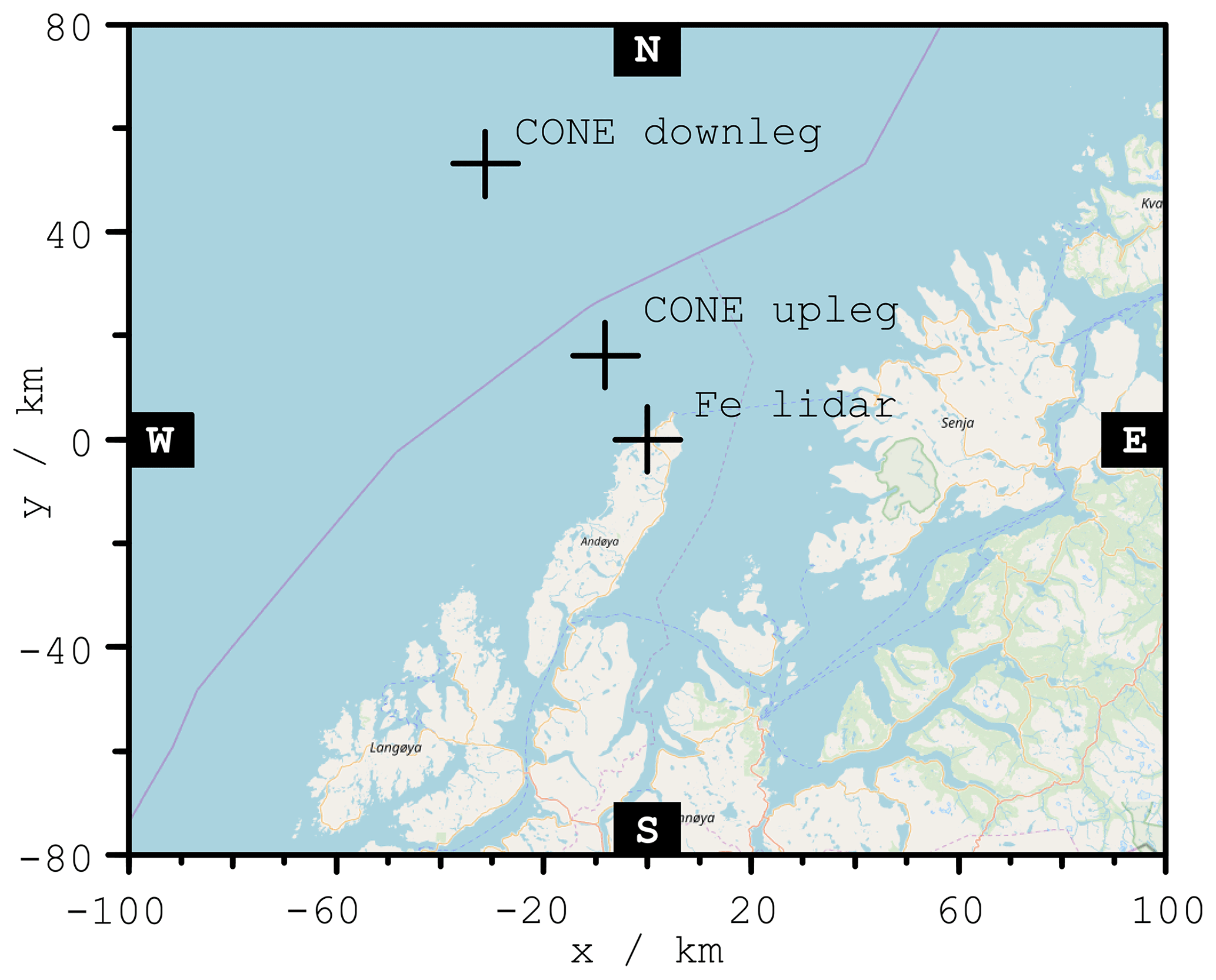
Figure 1Map showing the area covered by the AMTM at the centroid altitude of the OH layer at about 86 km. The points of measurement at that altitude are marked for each instrument (see text for further details).
The WADIS-2 rocket was launched from the Andøya Space Center in northern Norway (69∘ N, 14∘ E) on 5 March 2015 at 01:44 UT. Good weather conditions with clear sky in the period from 4 March 2015, 10:00 UT, to 5 March 2015, 12:00 UT, enabled simultaneous and nearly continuous Fe lidar and AMTM measurements with high data quality. No relevant ground-based optical measurements were obtained during the days before or after the launch due to poor weather conditions. In the following we focus on the discussion of data obtained within a 24 h period around the launch night, i.e. from 4 March 2014, 12:00 UT, to 5 March 2015, 12:00 UT.
3.1 WADIS-2 rocket (CONE)
Figure 2 shows the vertical temperature profiles obtained from the CONE measurements on the rocket payload. The horizontal distance of the up- and downleg measurements is around 50 km at an altitude of 86 km (see Fig. 1). The duration of the flight through the mesopause altitude range between 70 and 110 km is about 50 s for both the up- and downleg. In between the two profiles, the rocket spent about 2 min in the apogee range above 110 km. An effective altitude resolution of the temperature measurements with the CONE sensor is about 200 m (Rapp et al., 2003). The shapes of both profiles are very similar above 80 km and differ only in small details. The uncertainty is about 2 K at 70 km and increases with altitude (up to about 5 K at 110 km) (Strelnikov et al., 2013). For the most part the differences are within the uncertainty. The temperature shows two maxima at about 80 and 100 km. Such features are often referred to as “mesospheric inversion layers” (Hauchecorne and Maillard, 1992; Hauchecorne et al., 1987; Meriwether and Gerrard, 2004). The most prominent deviations between the profiles are of the order of 10 K and occur at around 95 and below 80 km.
3.2 Fe lidar
For direct comparison with the CONE data, the temperature profile obtained by the Fe lidar at the time of the rocket launch is shown in Fig. 2. In contrast to the in situ measurements, the Fe lidar data are integrated over 60 min and 1 km in altitude (with 0.2 km intervals) to derive a temperature profile. The centre of the averaging window is 01:45 UT.
Typical uncertainties are of the order of 2 K. At the edge of the layer, where metal densities are lower than in the centre and the backscatter signal is therefore weaker, the uncertainties are larger. Only temperatures with uncertainties not more than 10 K are shown. As shown in Fig. 1 for an altitude of 86 km, the distance of the Fe lidar profile to the upleg of the rocket is about 10 km. Therefore, the maximum distance between all three profiles is around 60 km. The temperature profile measured with the Fe lidar is in good agreement with the profiles measured with the CONE sensors on the rocket.
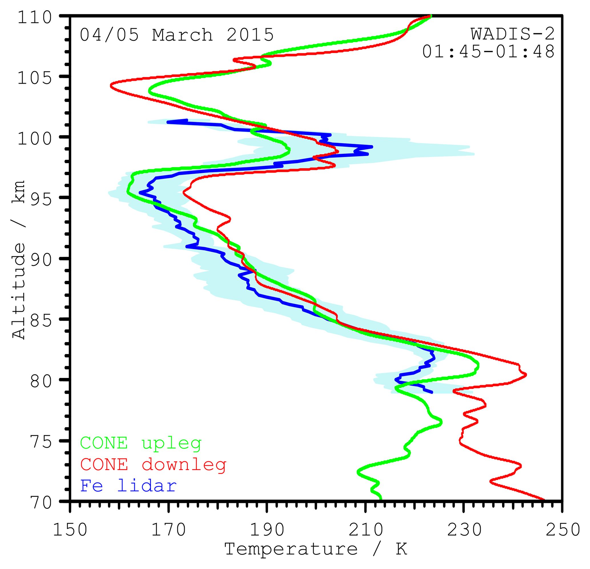
Figure 2Vertical temperature profiles at the launch time of the WADIS-2 rocket. The red and green curves show the in situ measurements with the rocket payload (CONE). The upleg (green) and the downleg (red) profiles are measured with two independent instruments at the ends of the payload. The Fe lidar (blue) profile is integrated over 60 min and centred at 01:45 UT. The blue shaded area shows the RMS of all Fe lidar profiles which have their centre within a period of ±60 min around launch time.
Figure 3 shows the temporal evolution of the temperatures in the mesopause region. Temperatures are calculated in 15 min and 0.2 km intervals using running means of 60 min and 1 km width, respectively. The observable altitude range as well as measurement uncertainties vary over time as absolute Fe densities and the vertical extent of the metal layer changes throughout the day (Höffner and Fricke-Begemann, 2005; Viehl et al., 2016).
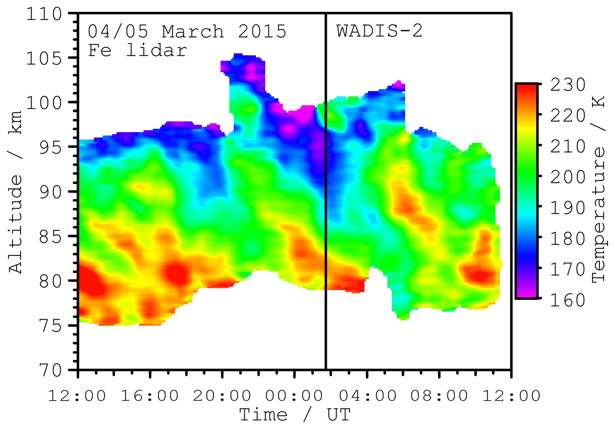
Figure 3Temperatures measured with the Fe lidar in the 24 h period around the WADIS-2 launch at 01:44 UT (vertical line). Measurement uncertainties are smaller than 10 K throughout the altitude range and decrease to around 2 K towards altitudes with the highest Fe density.
Figure 4 shows the mean temperature profile of the 24 h lidar measurement (see Fig. 3) compared to a profile calculated from the temperature climatology for the same day of the year. The climatology is calculated as described in Gerding et al. (2008) with a fit and includes about 2000 h of measurements since 2008 at Andøya. Mean temperatures during the observation period are typical for the polar mesopause region in the late winter state and the differences between the profiles are of the order of the day-to-day variability.
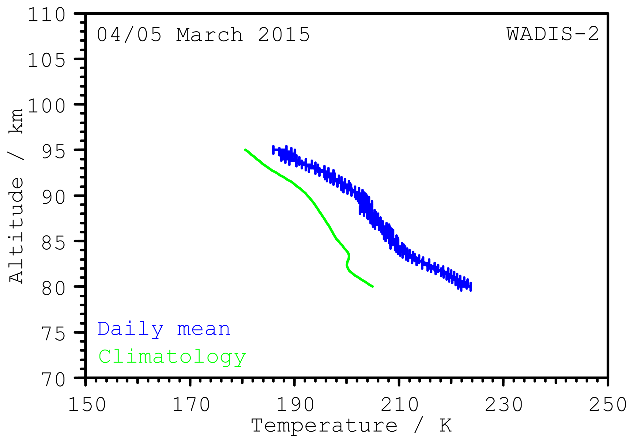
Figure 4Daily mean temperature profile (WADIS-2 day) compared to the profile from the climatology for the same day of the year. Only altitudes with 24 h observation time are shown.
Strong wave-like modulations with amplitudes of more than 30 K are clearly present. Lübken et al. (2011) observed similar wave-like modulations with the same instrument at the conjugate latitude in Antarctica. That study found surprisingly strong tidal signatures in temperature and Fe density observations with a harmonic analysis (24 and 12 h components) in summer. We perform a similar harmonic analysis to further investigate the apparent wave-like temperature structure in Fig. 3. The data shown in Fig. 3 are averaged in intervals of 60 min and 1 km vertical resolution. A non-linear function of sinusoidal components with fixed periods Pi is then fitted to the observations according to the relation
where Ai(z) are the amplitudes, Φi(z) the phases (at the time of the maximum amplitude), and z the altitude. In addition to the periods of 24 and 12 h investigated by Lübken et al. (2011), we also consider the higher harmonic 8 and 6 h components. All four components are optimised simultaneously but independently for each altitude using a least square fit routine. The seasonal variation in this analysis of 24 consecutive hours can be neglected contrary to the method presented by Lübken et al. (2011).
Figure 5 shows the result for the exemplary altitude of 86 km over time compared with the measurement. The main variation with large amplitudes is nearly fully described by the model using four components. The remaining variations are small compared to overall modulation which is of the order of 30 K. The mean squared error of the deviation is 4.6 K. The amplitudes for the 24 and the 12 h components are 4.8 and 2.8 K, respectively. The higher 8 and 6 h components show amplitudes of 6.5 and 1.4 K.

Figure 5Comparison of the temperature variations measured with the Fe lidar (blue) at an altitude of 86 km with the reconstruction (magenta) using the results of the harmonic wave analysis. The amplitudes of the 24, 12, 8, and 6 h components are 4.8, 2.8, 6.5, and 1.4 K.
Figure 6 shows the amplitudes and phases derived for all altitudes. Not all available temperature measurements shown in Fig. 3 are included here, as altitudes below 80 km and above 95 km are not fully covered throughout the 24 h observation period. The large amplitude of the 8 h component at all altitudes, which partly exceeds 10 K, is noteworthy, as is the strong 6 h component (above 87 km). Neither the 24 h nor the 12 h components reach comparable amplitudes. Altitudes at which the amplitudes of the harmonic fit is smaller than their uncertainty are removed in the phase plots. All four components show a clear phase progression in altitude without large phase jumps. This suggests clear waves in the data with periods near the chosen fit periods (24 h and higher harmonics). Since every altitude is fitted independently, random wave structures would lead to a more incoherent phase response and amplitude. A linear fit of the phase is used to estimate the phase slope for every component. A vertical wavelength and a phase are calculated using the slope and the position of the fitted lines at 86 km. Table 1 summarises the derived vertical wavelengths (λvertical) and the phases at 86 km. Phases are given in local solar time (LST), which was UT +51 min at the launch site on 5 March 2015. These values are calculated with a simple assumption of a linear phase progression with altitude. Due to the short available altitude range of only 15 km and the variability of the phase values with altitude (see Fig. 6) this can only be a rough estimation (without uncertainty). Generally the shape of the phase progression is not a straight line and the exact wavelength has to be identified from the distance between two extrema, which is not possible with our dataset.
Table 1Vertical wavelengths (λvertical) and phases (at 86 km) derived from the harmonic fit of Fe lidar temperatures.
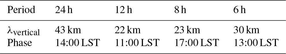
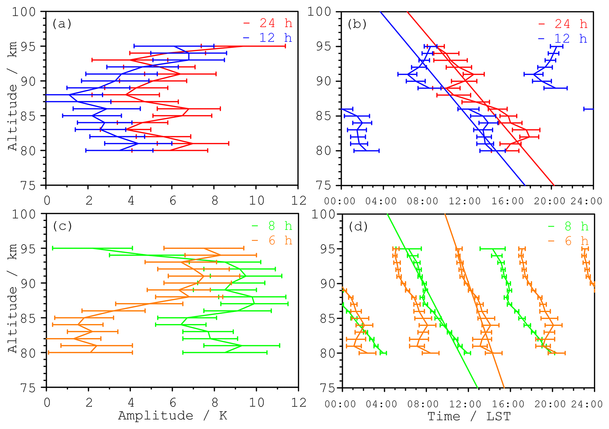
Figure 6Amplitudes (a, c) and phases (b, d) of the 24 h (red), 12 h (blue), 8 h (green), and 6 h (orange) wave components during the 24 h period around the WADIS-2 launch. The phase shift with altitude is approximated with straight lines and used to calculate vertical wavelengths. The approximation corresponds to vertical wavelength of 43 km for the 24 h, 22 km for the 12 h, 23 km for the 8 h, and 30 km for the 6 h component.
Figure 7 shows the deviation from the mean temperature at each altitude in comparison to the deviation of a temperature field reconstructed using only the components derived in the harmonic analysis. This reconstruction is in good agreement with the observations. The residuals do not exhibit any systematic deviations (not shown). Differences between measured and reconstructed temperatures mainly consist of small variations with periods smaller than 6 h, which are not considered in the fit.
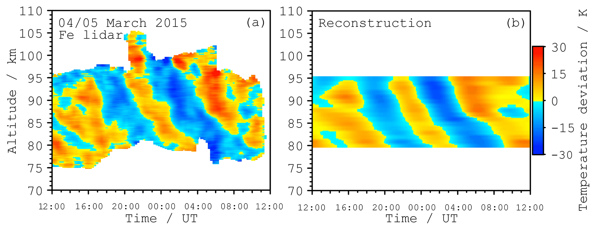
Figure 7Temperature observations with the Fe lidar (a) and the reconstruction using the four harmonic components (b) derived in the analysis.
3.3 Advanced Mesospheric Temperature Mapper (AMTM)
The AMTM provides horizontally resolved temperature maps during night-time conditions (sun more than 9∘ below the horizon). In early March, the first temperature maps are available at around 17:30 UT and observations end at around 05:00 UT. On the day of the WADIS-2 campaign, the data quality was somewhat affected by passing clouds between 22:00 and 24:00 UT as well as after 04:00 UT.
3.3.1 Horizontal temperature structure
Four representative examples of horizontal temperature maps are shown in Fig. 8. All panels show absolute temperatures (same scale with 30 K range). The boundary areas of the maps are partly shaded by other equipment on the roof or dust (the grey areas in the upper and lower part of the figures). Panels (a) and (b) are taken at 18:30 and 21:30 UT, that is, 7.2 and 4.2 h before the rocket launch. Panel (c) shows the temperature structure at the time of the rocket launch at 01:44 UT. This observation was taken 1 min before the launch, since the camera was overexposed due to the brightness of the rocket engine 1 min later. Panel (d) shows the situation at the end of the AMTM observations at 03:30 UT (1.8 h after rocket launch). Due to higher temperatures at the beginning of the observations (see Fig. 9 or 10) the temperature map in panel (a) (18:30 UT) is different from the other panels (more red and yellow instead of green and blue). These examples show only a slight increase or decrease at the edges and otherwise exhibit no systematic variations throughout the horizontal extent of the observations. In particular, the regions with vertical observations by CONE and Fe lidar (indicated by orange crosses, compare to Fig. 1) show only very small temperature variations. Observations with more gravity wave activity visible in AMTM maps are also available. Examples of common AMTM and lidar measurements with more gravity wave activity at the ALOMAR observatory can be found in Bossert et al. (2014), for example.
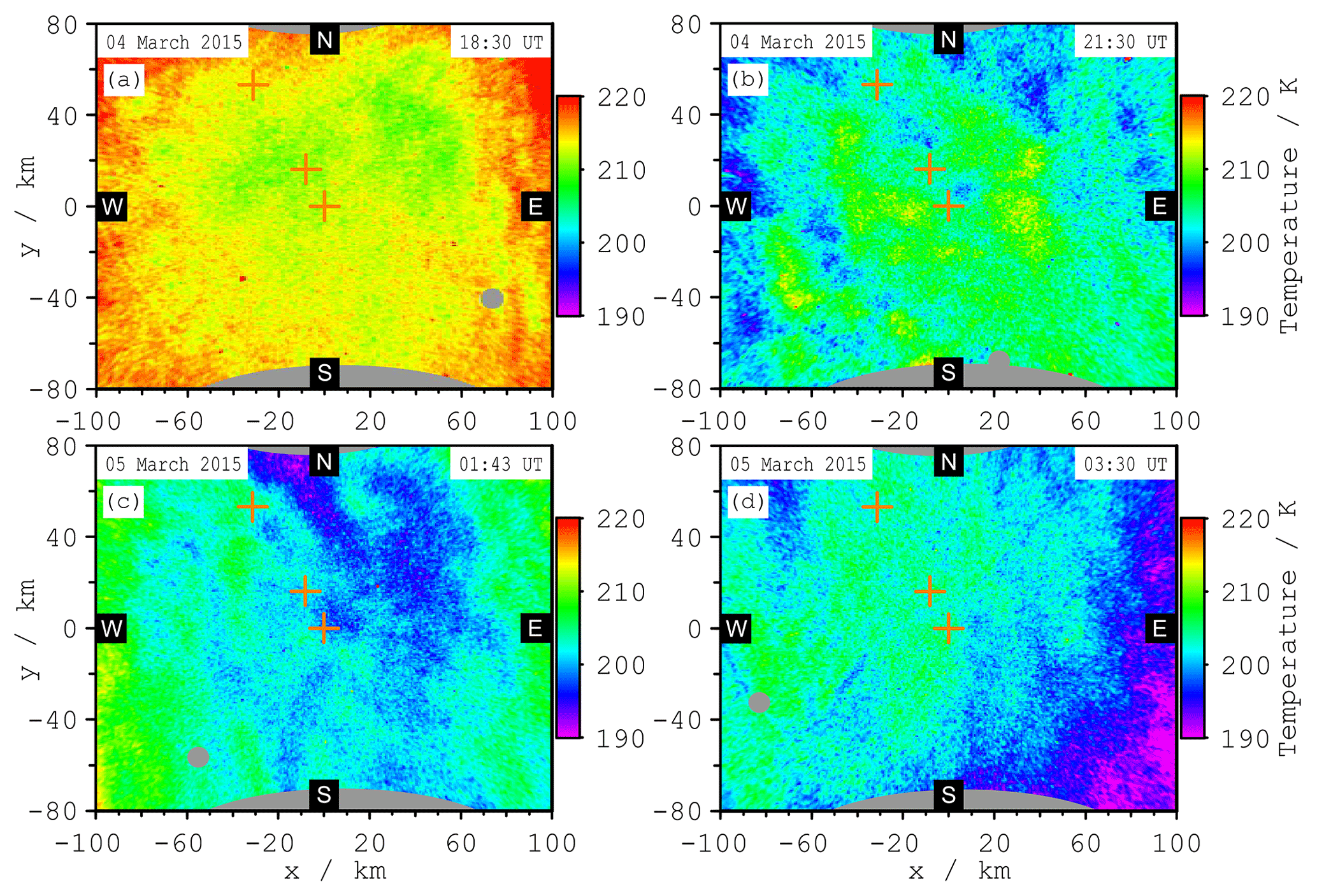
Figure 8Temperature maps measured with the AMTM. In (a), (b), and (d) the typical situation during the observation time is shown. (c) shows the situation at the rocket launch time. Very low gravity wave activity is apparent, which was the typical condition during this night.
Figure 9 shows the temporal evolution of the temperatures at different locations. The selected positions are the marked observation volumes of the other instruments (sub-array of 9 pixels×9 pixels which corresponds to about 5 km×5 km) and show the time-dependent OH temperature evolution measured by the AMTM. The time series is averaged by a 5 min running mean window shifted in 30 s intervals. The temperature differences between the selected locations does not vary significantly beyond the 2 K measurement uncertainty of the AMTM for most of the time. Temperature variations in time are dominated by long-term variations of several hours. There are also waves with periods around 5 min, but with small amplitudes of only a few kelvins (not shown). But they are disturbed from time to time by passing clouds. At the exact time of the launch, no temperature differences are discernible. The variations are nearly synchronous at all locations. The choice of the sub-array size (here 9 pixels×9 pixels) used to calculate a representative temperature for every position has nearly no effect on the results. A single pixel as well as an area larger than 9 pixels×9 pixels yields to nearly the same temperatures (not significantly different, not shown). This implies structures larger than the field of view (200 km×160 km) in the horizontal direction, since neither the average area size (sub-array) nor the position on the map have significant influence on the temperature results on this night.

Figure 9Temporal evolution of AMTM temperature observations derived from sub-arrays of 9 pixels×9 pixels (about 5 km×5 km) at the centre (blue), the rocket upleg (green), and the rocket downleg (red), respectively. The time series is smoothed with a Hanning filter of 5 min width.
3.3.2 Comparison of horizontal and vertical temperature observations
In Fig. 10, temperatures from AMTM observations are compared to vertical Fe lidar observations. An area of 9 pixels×9 pixels around the centre of the AMTM temperature map is taken and smoothed using a 60 min running mean window. That is the same time resolution as the Fe lidar temperatures (integration time of 60 min). Furthermore, a vertical averaging needs to be applied to the Fe lidar data to take the vertical profile of the OH layer and the subsequent altitude weighting of AMTM temperature measurements into account. However, the actual vertical extent of the OH layer during this observation is unknown. A Gaussian distribution with a constant full width half maximum (FWHM) of about 9 km is frequently assumed (Pautet et al., 2014; Zhao et al., 2005). This distribution is applied to the Fe lidar data as a weighting function, simulating the AMTM's vertical averaging throughout the OH layer. The centroid altitude of the weighting function is then shifted in altitude to find the best agreement between absolute AMTM and Fe lidar temperatures. The best agreement is found for the centroid altitude 84±1 km, where both instruments show the same temperatures within the error bars throughout the full observation period. This is a plausible altitude of the OH layer and hereafter assumed to be the mean altitude during the night. The best temperature agreement is found at a slightly higher centroid altitude of 85±1 km if relative temperature variations and not absolute temperatures are considered. However, this difference of 1 km (within the altitude uncertainty) is not significant for the following discussion as the weighting function smooths the values from different altitudes at a comparatively broad FWHM of 9 km. The exact knowledge of the OH layer altitude is not important for studies of horizontal structures, since relative temperatures are be used.
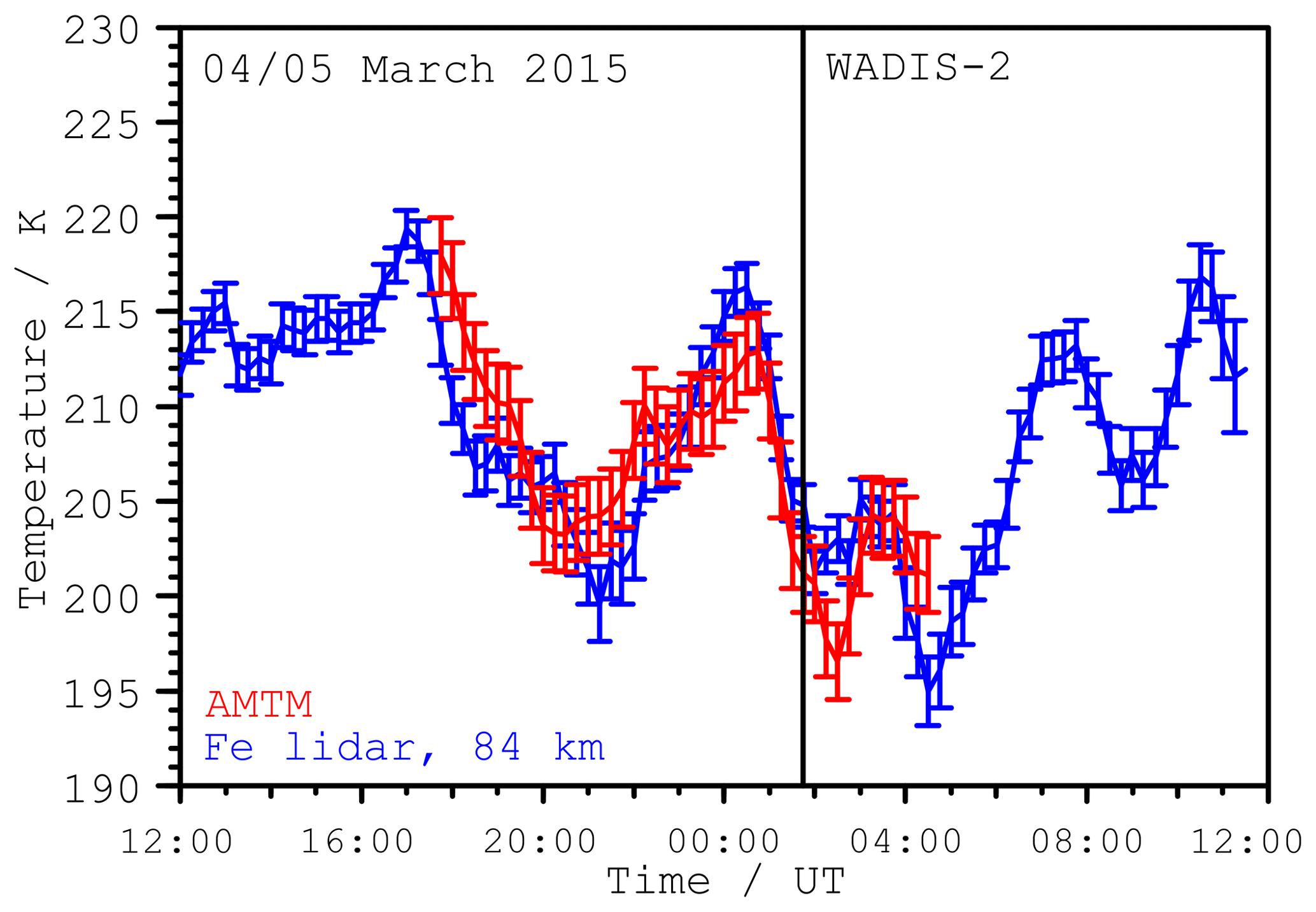
Figure 10Time series of OH temperatures (red) in comparison with the Fe lidar temperatures (blue). Lidar temperatures are averaged in altitude with a Gaussian weighting of 9 km FWHM and peak altitude of 84±1 km. Temperatures of the AMTM are taken from a sub-array of 9 pixels×9 pixels at the location of the Fe lidar and smoothed by a 60 min running mean.
The temperature profiles obtained by the CONE instrument during the up- and downleg (50 km distance) show a remarkably good agreement. The profiles are comparatively smooth above 80 km and only a few small structures disturb the dominating large structure. Small differences of about 5 K are observed at around 87 km or at 104 and 106 km. The uncertainty is about 2 K at 70 km, 5 K at 100 km, and 25 K at 110 km (Strelnikov et al., 2013). The CONE sensors measure the whole profile during the short flight time of about 50 s for the altitude range from 70 to 110 km. Waves with short periods are therefore not averaged out of the temperature profiles derived from the CONE instrument. While the up- and downleg temperature profiles are in good overall agreement above 80 km, they deviate from each other at lower altitudes. Small-scale structures with vertical sizes of several kilometres are largely absent at higher altitudes, but noticeable in the lower part. A possible explanation for the observed behaviour is an enhanced gravity wave activity at altitudes below 80 km. A more detailed analysis of the wave activity at lower altitudes is not possible with the given observations. Above 80 km altitude, the two profiles are also in very good agreement with the Fe lidar measurements. This is noteworthy since all three profiles were measured at different locations and are separated by a distance of up to 60 km. While the CONE sensors have a high time resolution, the Fe lidar profile is averaged over a 60 min period. The Fe lidar's measurement uncertainty is about 3 K in that altitude range. Due to the good agreement (within the uncertainties) and very similar variations of the three profiles, no variability at scales of the measurement distances can be identified. Dynamic structures larger than 60 km might be the reason.
Figure 2 additionally shows the RMS of Fe lidar temperature profiles (blue shaded area). The RMS is calculated from all profiles of the Fe lidar which have their centres within ±60 min around the launch (seven profiles, each integrated over 1 h). The temporal variability of the Fe lidar measurements is up to 20 K within only 1 h. This is significantly larger than the observed differences between the three profiles (or two instruments) at different horizontal locations. This means the phases of these three profiles are the same or deviate from each other by 2π or a multiple of it. The latter would mean wavelength of the order of 60 km (or shorter) and should be visible on AMTM temperature maps. Since the temperature maps show no such structures with the same large amplitudes than the temporal variations, they must have wavelengths significantly larger than 60 km.
The temporal evolution of the thermal structure in the mesopause region is obtained by analysing the full dataset of the Fe lidar. As noted above, the temperature structure is dominated by waves with comparatively long periods of 8 and 6 h. This occasionally causes vertical temperature profiles that do not follow the simple model of a mesopause region with a negative temperature gradient below and a positive temperature gradient above. Such inverted temperature profiles are sometimes referred to as “mesospheric inversion layers” and occur quite regularly in the presence of strong waves with long periods (Meriwether and Gardner, 2000). A harmonic analysis demonstrates that the main variability is given by only four harmonic components (24, 12, 8, and 6 h), adding up to more than 30 K temperature difference. In addition to these four components, only waves with periods smaller than 6 h remain. We note that the dataset that the harmonic analysis is performed on is not sensitive to waves with periods smaller than about 2 h due to the 60 min integration time of the Fe lidar temperatures.
Fe lidar measurements with the same instrument at the opposite latitude in the Southern Hemisphere at Davis, Antarctica (69∘ S), had revealed clear and regular 24 h (diurnal) and 12 h (semi-diurnal) tides with large amplitudes (Lübken et al., 2011). During the WADIS-2 campaign we find a dominating 8 h wave structure. An additional strong 6 h component may also be present above 87 km. In contrast to the observations in the Southern Hemisphere, 24 and 12 h variations were comparatively weak. We note that this current analysis is limited to a single day (24 h) and not a composite of 180 h of measurements during a period of 12 days as in Lübken et al. (2011). Due to the high variability in tidal phases and amplitudes (Baumgarten et al., 2018; Murphy et al., 2006) the results of a single day (our dataset) are expected to deviate to some extent in phase (several hours) and amplitude from an average (Lübken et al., 2011).
The presence of clear 24 and 12 h tides as reported in Lübken et al. (2011) for Davis suggests that tides could be an explanation for the measured 24 and 12 h waves. Nevertheless, gravity waves have to be taken into account, in particular for the higher frequency components. It is not possible to exclude them but there are some arguments for tides we discuss below. With the analysis of the phase progression (see Fig. 6) an estimation of the vertical wavelength and the phase are possible. A vertical wavelength of 43 km for the 24 h wave and 22 km for the 12 h wave is found in this study. The phase of the 24 h component at 86 km derived in this study has a maximum at about 14:00 LST, the 12 h compound at about 11:00 LST. The data used in Lübken et al. (2011) were obtained at different locations (Southern instead of Northern Hemisphere) and also during a different season (summer instead of spring). Therefore, a more detailed comparison does not necessarily result in a good agreement due to the seasonal variability. Lübken et al. (2011), however, report only a slightly different vertical wavelength of 30 km for observations of 24 h temperature tides and 40 km for tides in Fe densities, as well as a phase maximum at 86 km at 13:00 LST. Model calculations for thermal tides were done for temperatures, e.g. for 24 h by Forbes (1982a) and for 12 h by Forbes (1982b) at 60∘ latitude during equinox conditions. The phase progressions reported in Forbes (1982a, b) are used to estimate the phase and vertical wavelength for the 24 and 12 h tide in the same way. Vertical wavelength (at about 90 km) in the range of 30–35 km for the 24 h tide is similar to the findings of 43 km in this study, while the range of 20–30 km for the 12 h tide is in good agreement with the findings of 22 km, in this study. A comparison of the phase does not add up to a clear result. The phase maximum of the 24 h tide (08:00 LST) calculated by Forbes (1982a) differs significantly from our finding (14:00 LST), the phase maximum of the 12 h tide (14:00 LST, Forbes (1982b)) differs slightly from our result (11:00 LST). The model calculations in Forbes (1982a, b) do not include short-term variability in tides, and also the difference in latitude (Forbes 60∘, this study 69∘) might be the reason for the differences. The short available dataset in this study (24 h) can also explain the differences, especially for the 24 h tide, since the dataset covers only one period to fit. Nevertheless, the rough agreement of the model calculations, the results in Lübken et al. (2011) and the WADIS-2 dataset in this study allow a presumption that at least the 24 and the 12 h waves are of tidal origin.
Winds from radar measurements and temperatures from airglow measurements at polar latitudes are discussed relating the 8 h and the 6 h tides (Dalin et al., 2017; Smith et al., 2004; Wu et al., 2005; Younger et al., 2002). In contrast to our results the higher harmonic components (8 and 6 h) were found to be significantly smaller than the 24 and 12 h tides. Vertical wavelength in the range of 25 to 45 km (spring) are reported for the 8 h tide (Wu et al., 2005; Younger et al., 2002). This is in good agreement with our finding of 23 km. The 30 to 50 km range for the 6 h tide as reported in Smith et al. (2004) is also in good agreement with our result of 30 km and might suggest that the strong 8 and 6 h components found in this paper are tides. In contrast to the good agreement in vertical wavelength the large amplitudes of the 8 and 6 h waves are unexpected. Higher harmonic tides, in particular the 8 h component, are discussed in several theoretical papers (Akmaev, 2001; Batista et al., 2004; Beldon et al., 2006; Jacobi and Fytterer, 2012; Lilienthal et al., 2018; Smith et al., 2004; States and Gardner, 2000; Taylor et al., 1999; Thayaparan, 1997; Wu et al., 2005; Younger et al., 2002). Generally the amplitude of the 8 h component and higher harmonics are assumed to be significantly smaller than the 24 and 12 h components. A small number of publications report 8 h tides with large amplitudes (Taylor et al., 1999; Thayaparan, 1997), but at mid-latitudes. They also report an 8 h tidal component with amplitudes smaller compared to the 24 h and the 12 h component in averaged datasets. However, single events (days) with 8 h tides and amplitudes larger than the 24 h and the 12 h tides are described, too.
Some good reasons can be found that not only the 24 and the 12 h waves but also the strong 8 h and the 6 h waves are tides, as described above. However, a larger dataset with global coverage is necessary to determine the temporal and the spatial structure, and to separate the tidal and the gravity wave components unambiguously.
In addition to the vertical information provided by the CONE and Fe lidar instruments, horizontal information can be extracted from the AMTM temperature maps. The AMTM measurements are limited to the OH layer altitude. While this is only a single altitude or rather an altitude range of about 9 km (FWHM) due to the thickness of the OH layer, the analysis reveals interesting horizontal structures. A peak altitude of the OH layer at about 85 km and a FWHM of 9 km are typical values and seem to be good estimates since both absolute temperatures and the structures in the time series show a good agreement with the Fe lidar. Without the presence of small structures (with large amplitudes), like gravity waves, the large structures should dominate the horizontal AMTM temperature maps. In Bossert et al. (2014) and Pautet et al. (2014) some examples of typical AMTM observations with gravity wave activity are described. Figure 8 shows the typical situation during the night of the WADIS-2 launch. In contrast to other examples (Bossert et al., 2014; Pautet et al., 2014) only apparently random small structures are visible. The whole map shows temperature differences of no more than 10 K. This does not exclude the presence of smaller perturbations. Because temperatures are derived from the OH layer with a thickness of about 9 km, vertical structures of a similar size or smaller than the layer width cannot be resolved. A simple way to estimate the relation between datasets measured at different locations in a time series is to pick the temperatures at the locations of interest in the AMTM maps and compare them. Figure 9 shows an impressive synchronous evolution at all locations at a resolution of 5 min. Taking the measurement uncertainty of the AMTM of about 2 K into account, there are only a few short periods where the deviations are significant. From time to time, e.g. at around 22:00 UT and at about 04:00 UT, the deviations are due to clouds. Comparing the different locations in the horizontally resolved AMTM temperature maps shows that the large structures found in all vertical profiles are not only long term, but have also large horizontal scales since no systematic deviation or change in temperature was observed in horizontal direction. Clearly, a dynamic variation with a horizontal extent larger than the field of view of the AMTM, which corresponds to an area of about 200 km×160 km, was present around the time of the WADIS-2 launch. Large structures in the horizontal direction are in principle an indication of tidal structures. However, the field of view is limited to 200 km×160 km and it is not possible to exclude gravity waves with horizontal wavelengths of the same order.
Temperatures derived from the Doppler-broadening of metal atoms with the Fe lidar and from excited rotational OH (3,1) transitions with the AMTM are in very good agreement to each other. Both the absolute temperatures and the deviation during the observation period suggest an OH centroid altitude between 84 and 86 km. However, in the context of this paper such statements refer only to the observation in this single night and the assumption of a fixed altitude and layer shape is not justified in all cases (Dunker, 2018; Grygalashvyly et al., 2014; Liu and Shepherd, 2006; Melo et al., 2000; Perminov et al., 1999; Zhao et al., 2005).
We have analysed the temperature structure in the mesopause region during the WADIS-2 rocket campaign in March 2015. Temperatures in the night of the rocket launch were dominated by larger waves at 8 and 6 h periods and waves of smaller scales play only a minor role. The lidar measurements show waves with typical periods for 24 and 12 h tides. A strong 8 h wave (and at higher altitudes also a 6 h wave) is dominating the variations in temperatures and might also be tides. Amplitudes of up to 10 K for this single harmonic component exceed the corresponding amplitudes of the longer 24 and 12 h components of 6 K. Disturbances by waves or other structures with smaller periods have only small amplitudes and play a minor role.
On this night the small-scale gravity wave activity was limited to comparatively small amplitudes of only a few kelvins in the horizontal AMTM measurements. The long periodic tidal-like variations in time domain show no structures in the observable area of 160 km×200 km. The structure size of the dynamic variation dominating this night has to be larger than 200 km, as temperatures change quasi-synchronously at all locations. As a result of this situation, the rocket-borne measurements show two vertical temperature profiles with very similar structures, although they were measured at a horizontal distance of 50 km.
The Fe lidar, which was located 10 km away from the WADIS-2 measurements, provides further vertical temperature profiles which show the same features as the profiles measured with CONE during the rocket flight. In particular, the altitude range around the OH layer at about 85 km shows the same structures and absolute temperatures.
In this case the OH temperatures show a remarkably good agreement with the lidar temperatures during the whole night, if we assume an OH density centroid altitude of 85 km. Below 80 km stronger temperature deviations as well as small variations are the result of the increasing influence of small-scale gravity waves.
Data are available at ftp://ftp.iap-kborn.de/data-in-publications/WoerlACP2018/, last access: 30 November 2018.
BS coordinated the WADIS project, provided the CONE temperature data and contributed to their analysis and discussions. PDP provided the AMTM data. PDP, MJT, and YZ contributed to their analysis and discussions. JH and RW provided the Fe lidar data and contributed to their analysis and discussions. TPV, JH, and FJL contributed to the discussion of the results and the paper. RW analysed the data and prepared the paper with feedback of the co-authors.
The authors declare that they have no conflict of interest.
This article is part of the special issue “Sources, propagation, dissipation and impact of gravity waves (ACP/AMT inter-journal SI)”. It is not associated with a conference.
This work was supported by the German Space Agency (DLR) under grant 50OE1001
(project WADIS). The design and initial development of the AMTM was supported
under the AFOSR DURIP grant F49620-02-1-0258. Its installation and operations
at ALOMAR were supported under the NSF collaborative grant AGS-1042227. This
project was also partly supported by the Deutsche Forschungsgemeinschaft
(DFG, German Research Foundation) under project LU1174/8-1 (PACOG), FOR1898
(MS-GWaves). The work was also partly supported by the Bundesministerium
für Bildung und Forschung (BMBF, Federal Ministry of Education and
Research) under project D/553/67210010 (ROMIC-GWLcycle).
The publication of this article was funded by the
Open Access Fund of the Leibniz Association.
Edited by: Jörg Gumbel
Reviewed by: two anonymous referees
Akmaev, R. A.: Seasonal variations of the terdiurnal tide in the mesosphere and lower thermosphere: A model study, Geophys. Res. Lett., 28, 3817–3820, https://doi.org/10.1029/2001GL013002, 2001. a
Baker, D. J. and Stair, A. T.: Rocket measurements of the altitude distributions of the hydroxyl airglow, Phys. Scr., 37, 611, 1988. a
Batista, P. P., Clemesha, B. R., Tokumoto, A. S., and Lima, L. M.: Structure of the mean winds and tides in the meteor region over Cachoeira Paulista, Brazil (22.7∘ S, 45∘ W) and its comparison with models, J. Atmos. Sol.-Terr. Phy., 66, 623–636, https://doi.org/10.1016/j.jastp.2004.01.014, 2004. a
Baumgarten, K., Gerding, M., Baumgarten, G., and Lübken, F.-J.: Temporal variability of tidal and gravity waves during a record long 10-day continuous lidar sounding, Atmos. Chem. Phys., 18, 371–384, https://doi.org/10.5194/acp-18-371-2018, 2018. a
Beldon, C. L., Muller, H. G., and Mitchell, N. J.: The 8-hour tide in the mesosphere and lower thermosphere over the UK, 1988–2004, J. Atmos. Sol.-Terr. Phy., 68, 655–668, https://doi.org/10.1016/j.jastp.2005.10.004, 2006. a
Bossert, K., Fritts, D., Pautet, P., Taylor, M. J., Williams, B., and Pendelton, W. R.: Investigation of a mesospheric gravity wave ducting event using coordinated sodium lidar and Mesospheric Temperature Mapper measurements at ALOMAR, Norway (69∘ N), J. Geophys. Res.-Atmos., 119, 16, https://doi.org/10.1002/2014JD021460, 2014. a, b, c
Chapman, S. and Lindzen, R. S.: Atmospheric Tides: Thermal and Gravitational, Gordon and Breach New York, 1970. a
Dalin, P., Kirkwood, S., Pertsev, N., and Perminov, V.: Influence of Solar and Lunar Tides on the Mesopause Region as Observed in Polar Mesosphere Summer Echoes Characteristics, J. Geophys. Res.-Atmos., 122, 10369–10383, https://doi.org/10.1002/2017JD026509, 2017. a
Dunker, T.: The airglow layer emission altitude cannot be determined unambiguously from temperature comparison with lidars, Atmos. Chem. Phys., 18, 6691–6697, https://doi.org/10.5194/acp-18-6691-2018, 2018. a
Eckermann, S. D. and Marks, C. J.: An idealized ray model of gravity wave–tidal interactions, J. Geophys. Res.-Atmos., 101, 21195–21212, https://doi.org/10.1029/96JD01660, 1996. a
Forbes, J. M.: Atmospheric tides: 1. Model description and results for the solar diurnal component, J. Geophys. Res.-Space Phys., 87, 5222–5240, https://doi.org/10.1029/JA087iA07p05222, 1982a. a, b, c, d
Forbes, J. M.: Atmospheric tide: 2. The solar and lunar semidiurnal components, J. Geophys. Res.-Space Phys., 87, 5241–5252, https://doi.org/10.1029/JA087iA07p05241, 1982b. a, b, c, d
Forbes, J. M.: Middle atmosphere tides, J. Atmos. Terr. Phys., 46, 1049–1067, https://doi.org/10.1016/0021-9169(84)90008-4, 1984. a
Fritts, D. C. and Alexander, M. J.: Gravity wave dynamics and effects in the middle atmosphere, Rev. Geophys., 41, 1, https://doi.org/10.1029/2001RG000106, 2003. a
Gerding, M., Höffner, J., Lautenbach, J., Rauthe, M., and Lübken, F.-J.: Seasonal variation of nocturnal temperatures between 1 and 105 km altitude at 54∘ N observed by lidar, Atmos. Chem. Phys., 8, 7465–7482, https://doi.org/10.5194/acp-8-7465-2008, 2008. a
Giebeler, J., Lübken, F.-J., and Nägele, M.: CONE - a new sensor for in-situ observations of neutral and plasma density fluctuations, Montreux93, ESA-SP-355, 311–318, 1993. a, b
Grygalashvyly, M., Sonnemann, G. R., Lübken, F.-J., Hartogh, P., and Berger, U.: Hydroxyl layer: mean state and trends at mid latitudes, J. Geophys. Res.-Atmos., 119, 12391–12419, https://doi.org/10.1002/2014JD022094, 2014. a
Hagan, M. E. and Forbes, J. M.: Migrating and nonmigrating diurnal tides in the middle and upper atmosphere excited by tropospheric latent heat release, J. Geophys. Res.-Atmos., 107, ACL 6-1–ACL 6-15, https://doi.org/10.1029/2001JD001236, 2002. a
Hauchecorne, A. and Maillard, A.: The mechanism of formation of inversion layers in the mesosphere, Adv. Space Res., 12, 219–223, 1992. a
Hauchecorne, A., Chanin, M. L., and Wilson, R.: Mesospheric temperature inversion and gravity wave breaking, Geophys. Res. Lett., 14, 933–936, https://doi.org/10.1029/GL014i009p00933, 1987. a
Höffner, J. and Fricke-Begemann, C.: Accurate lidar temperatures with narrowband filters, Opt. Lett., 30, 890–892, https://doi.org/10.1364/OL.30.000890, 2005. a
Höffner, J. and Lautenbach, J.: Daylight measurements of mesopause temperature and vertical wind with the mobile scanning iron Lidar, Opt. Lett., 34, 1351–1353, 2009. a
Jacobi, Ch. and Fytterer, T.: The 8-h tide in the mesosphere and lower thermosphere over Collm (51.3∘ N; 13.0∘ E), 2004–2011, Adv. Radio Sci., 10, 265–270, https://doi.org/10.5194/ars-10-265-2012, 2012. a
Lautenbach, J. and Höffner, J.: Scanning iron temperature lidar for mesopause temperature observation, Appl. Optics, 43, 4559–4563, https://doi.org/10.1364/AO.43.004559, 2004. a, b
Lilienthal, F., Jacobi, C., and Geißler, C.: Forcing mechanisms of the terdiurnal tide, Atmos. Chem. Phys., 18, 15725–15742, https://doi.org/10.5194/acp-18-15725-2018, 2018. a
Liu, G. and Shepherd, G. G.: An empirical model for the altitude of the OH nightglow emission, Geophys. Res. Lett., 33, 9, https://doi.org/10.1029/2005GL025297, 2006. a
Lübken, F.-J., Höffner, J., Viehl, T. P., Kaifler, B., and Morris, R. J.: First measurements of thermal tides in the summer mesopause region at Antarctic latitudes, Geophys. Res. Lett., 38, 24, https://doi.org/10.1029/2011GL050045, 2011. a, b, c, d, e, f, g, h, i, j
Melo, S. M. L., Lowe, R. P., and Russell, J. P.: Double-peaked hydroxyl airglow profiles observed from WINDII/UARS, J. Geophys. Res.-Atmos., 105, 12397–12403, https://doi.org/10.1029/1999JD901169, 2000. a
Meriwether, J. and Gerrard, A. J.: Mesosphere inversion layers and stratosphere temperature enhancements, Rev. Geophys., 42, 3, https://doi.org/10.1029/2003RG000133, 2004. a
Meriwether, J. W. and Gardner, C. S.: A review of the mesosphere inversion layer phenomenon, J. Geophys. Res., 105, 12405–12416, https://doi.org/10.1029/2000JD900163, 2000. a
Murphy, D. J., Forbes, J. M., Walterscheid, R. L., Hagan, M. E., Avery, S. K., Aso, T., Fraser, G. J., Fritts, D. C., Jarvis, M. J., McDonald, A. J., Riggin, D. M., Tsutsumi, M., and Vincent, R. A.: A climatology of tides in the Antarctic mesosphere and lower thermosphere, J. Geophys. Res.-Atmos., 111, D23, https://doi.org/10.1029/2005JD006803, 2006. a
Pautet, P.-D., Taylor, M. J., Pendleton, W. R., Zhao, Y., Yuan, T., Esplin, R., and McLain, D.: Advanced mesospheric temperature mapper for high-latitude airglow studies, Appl. Optics, 53, 5934–5943, https://doi.org/10.1364/AO.53.005934, 2014. a, b, c, d, e
Perminov, V., Lowe, R., and Pertsev, N.: Longitudinal variations in the hydroxyl nightglow, Adv. Space Res., 24, 1609–1612, https://doi.org/10.1016/S0273-1177(99)00887-X, 1999. a
Rapp, M., Gumbel, J., and Lübken, F.-J.: Absolute density measurements in the middle atmosphere, Ann. Geophys., 19, 571–580, https://doi.org/10.5194/angeo-19-571-2001, 2001. a
Senf, F. and Achatz, U.: On the impact of middle-atmosphere thermal tides on the propagation and dissipation of gravity waves, J. Geophys. Res.-Atmos., 116, D24, https://doi.org/10.1029/2011JD015794, 2011. a
Smith, A. K.: Global Dynamics of the MLT, Surv. Geophys., 33, 1177–1230, https://doi.org/10.1007/s10712-012-9196-9, 2012. a
Smith, A. K., Pancheva, D., and Mitchell, N.: Observations and modeling of the 6-hour tide in the upper mesosphere, J. Geophys. Res., 109, D10, https://doi.org/10.1029/2003JD004421, 2004. a, b, c
States, R. J. and Gardner, C. S.: Thermal structure of the mesopause region (80–105 km) at 40∘ N latitude. Part I: Seasonal variations, J. Atmos. Sci., 57, 66–77, https://doi.org/10.1175/1520-0469(2000)057<0066:TSOTMR>2.0.CO;2, 2000. a
Strelnikov, B., Rapp, M., and Lübken, F.-J.: In-situ density measurements in the mesosphere/lower thermosphere region with the TOTAL and CONE instruments, in: An Introduction to Space Instrumentation, edited by: Oyama, K., Terra Publishers, Tokyo, https://doi.org/10.5047/aisi.001, 2013. a, b, c, d
Strelnikov, B., Szewczyk, A., Strelnikova, I., Latteck, R., Baumgarten, G., Lübken, F.-J., Rapp, M., Fasoulas, S., Löhle, S., Eberhart, M., Hoppe, U.-P., Dunker, T., Friedrich, M., Hedin, J., Khaplanov, M., Gumbel, J., and Barjatya, A.: Spatial and temporal variability in MLT turbulence inferred from in situ and ground-based observations during the WADIS-1 sounding rocket campaign, Ann. Geophys., 35, 547–565, https://doi.org/10.5194/angeo-35-547-2017, 2017. a, b
Taylor, M. J., Pendleton, W. R., Gardner, C. S., and States, R. J.: Comparison of terdiurnal tidal oscillations in mesospheric OH rotational temperature and Na lidar temperature measurements at mid-latitudes for fall/spring conditions, Earth Planet. Space, 51, 877–885, https://doi.org/10.1186/BF03353246, 1999. a, b
Thayaparan, T.: The terdiurnal tide in the mesosphere and lower thermosphere over London, Canada (43∘ N, 81∘ W), J. Geophys. Res.-Atmos., 102, 21695–21708, https://doi.org/10.1029/97JD01839, 1997. a, b
Viehl, T. P., Plane, J. M. C., Feng, W., and Höffner, J.: The photolysis of FeOH and its effect on the bottomside of the mesospheric Fe layer, Geophys. Res. Lett., 43, 1373–1381, https://doi.org/10.1002/2015GL067241, 2016. a, b
von Zahn, U., Fricke, K. H., Gerndt, R., and Blix, T.: Mesospheric temperatures and the OH layer height as derived from ground-based lidar and OH* spectrometry, J. Atmos. Sol.-Terr. Phy., 49, 863–869, https://doi.org/10.1016/0021-9169(87)90025-0, 1987. a
Wu, Q., Mitchell, N. J., Killeen, T. L., Solomon, S. C., and Younger, P. T.: A high-latitude 8-hour wave in the mesosphere and lower thermosphere, J. Geophys. Res.-Space Phys., 110, A9, https://doi.org/10.1029/2005JA011024, 2005. a, b, c
Younger, P. T., Pancheva, D., Middleton, H. R., and Mitchell, N. J.: The 8-hour tide in the Arctic mesosphere and lower thermosphere, J. Geophys. Res., 107, 1420, https://doi.org/10.1029/2001JA005086, 2002. a, b, c
Zhao, Y., Taylor, M. J., and Chu, X.: Comparison of simultaneous Na lidar and mesospheric nightglow temperature measurements and the effects of tides on the emission layer heights, J. Geophys. Res.-Atmos., 110, d09S07, https://doi.org/10.1029/2004JD005115, 2005. a, b