the Creative Commons Attribution 4.0 License.
the Creative Commons Attribution 4.0 License.
 | 22 Jan 2019
Dynamically controlled ozone decline in the tropical mid-stratosphere observed by SCIAMACHY
Evgenia Galytska
Alexey Rozanov
Martyn P. Chipperfield
Sandip. S. Dhomse
Mark Weber
Carlo Arosio
Wuhu Feng
John P. Burrows
Despite the recently reported beginning of a recovery in global stratospheric ozone (O3), an unexpected O3 decline in the tropical mid-stratosphere (around 30–35 km altitude) was observed in satellite measurements during the first decade of the 21st century. We use SCanning Imaging Absorption spectroMeter for Atmospheric CHartographY (SCIAMACHY) measurements for the period 2004–2012 to confirm the significant O3 decline. The SCIAMACHY observations show that the decrease in O3 is accompanied by an increase in NO2.
To reveal the causes of these observed O3 and NO2 changes, we performed simulations with the TOMCAT 3-D chemistry-transport model (CTM) using different chemical and dynamical forcings. For the 2004–2012 time period, the TOMCAT simulations reproduce the SCIAMACHY-observed O3 decrease and NO2 increase in the tropical mid-stratosphere. The simulations suggest that the positive changes in NO2 (around 7 % decade−1) are due to similar positive changes in reactive odd nitrogen (NOy), which are a result of a longer residence time of the source gas N2O and increased production via N2O + O(1D). The model simulations show a negative change of 10 % decade−1 in N2O that is most likely due to variations in the deep branch of the Brewer–Dobson Circulation (BDC). Interestingly, modelled annual mean “age of air” (AoA) does not show any significant changes in transport in the tropical mid-stratosphere during 2004–2012.
However, further analysis of model results demonstrates significant seasonal variations. During the autumn months (September–October) there are positive AoA changes that imply transport slowdown and a longer residence time of N2O allowing for more conversion to NOy, which enhances O3 loss. During winter months (January–February) there are negative AoA changes, indicating faster N2O transport and less NOy production. Although the variations in AoA over a year result in a statistically insignificant linear change, non-linearities in the chemistry–transport interactions lead to a statistically significant negative N2O change.
- Article
(8745 KB) - Full-text XML
-
Supplement
(1181 KB) - BibTeX
- EndNote


Stratospheric ozone (O3) is one of the most important components of the atmosphere. It absorbs ultraviolet solar radiation, which is harmful to plants, animals, and humans, and thereby plays a key role in determining the thermal structure and dynamics of the stratosphere (Jacobson, 2002; Seinfeld and Pandis, 2006). The amount of O3 in the stratosphere is controlled by a balance between photochemical production and loss mechanisms. However, the atmospheric dynamics play an important role in determining the conditions at which these photochemical and chemical reactions take. As a result O3 global distribution and inter-annual variability are governed by transport processes, e.g. the Brewer–Dobson Circulation (BDC). To set the scene for our understanding of chemical O3 variations in the tropical mid-stratosphere, we briefly discuss the mechanism of O3 production and loss via catalytic NOx (NOx = NO + NO2) cycle and the role of nitrous oxide (N2O).
Stratospheric O3 is essentially formed in the regions where solar ultraviolet electromagnetic radiation is present (Chapman, 1930). The first mechanism proposed to explain its formation and loss is known as the Chapman cycle. O3 is formed via photodissociation of molecular oxygen (O2) mostly within the so-called Herzberg continuum (200–242 nm; Nicolet, 1981). Absorption by O2 at shorter wavelengths (e.g. Schumann–Runge bands, 175–200 nm) occurs at higher altitudes, i.e. in the upper stratosphere and mesosphere. In the mid-stratosphere the ultraviolet sunlight breaks apart an O2 molecule to produce two oxygen (O) atoms:
Then each O atom combines with O2 to produce O3:
where M represents a third body. Reactions (R1) and (R2) continually occur whenever shortwave ultraviolet radiation is present in the stratosphere. As a consequence, the strongest O3 production takes place in the tropical mid-stratosphere. Then O3 is photolysed with lower-energy photons in the Hartley bands (242–310 nm) to produce excited singlet oxygen (O(1D)) or in the Huggins band (310–400 nm) to produce ground-state atomic oxygen O(3P):
An important aspect of O3 photochemistry is that it is the major source of O(1D) in the stratosphere Reaction (R3a). O(1D) is rapidly quenched to the electronic ground state by collision with any third-body molecule, most likely N2 or O2 (O(1D) + M → O + M; Jacob, 1999). The final Chapman cycle reaction of O3 and atomic oxygen Reaction (R4) is relatively slow and does not cause significant O3 loss, since O2 recombines with an O atom to regenerate O3 via Reaction (R2).
Importantly, other chemical cycles can catalyse this reaction.
The distribution of O3 in the stratosphere is illustrated in Fig. 1. Panel (a) shows zonally averaged climatological mean O3 volume mixing ratio (vmr) as a function of latitude in the stratosphere from SCIAMACHY measurements (further described in Sect. 2.1) during boreal winters (December–January–February, DJF) 2004–2012. We chose Northern Hemisphere winter months to clearly represent the hemispheric distributions of O3. Figure 1b shows the mean O3 vertical profile for the tropical region, averaged for the same period as in panel a. The dashed rectangles indicate the region of the tropical (10∘ S–10∘ N) mid-stratosphere (30–35 km) investigated in this study.
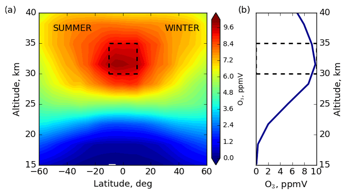
Figure 1SCIAMACHY zonally averaged climatological mean O3 (ppmV) for (a) latitude–altitude distribution and (b) profile during DJFs 2004–2012. The dashed rectangles indicate the region of tropical mid-stratosphere investigated in this paper.
Significant O3 destruction occurs through reaction with oxides of nitrogen (NOx, whose major source is N2O), hydrogen (HOx = OH, H2O, whose major sources are CH4 and H2O), chlorine (ClOx, whose major sources are chlorofluorocarbons, known as CFCs, and other halocarbons), and bromine (BrOx, whose major sources are methyl bromide and halons). Portmann et al. (2012) showed that the relative mean global O3 loss in the upper and lower stratosphere is dominated by the HOx and ClOx∕BrOx chemistry, and in the middle stratosphere by the NOx cycle, which is largest near the O3 maximum. Consequently, significant O3 loss in the tropical mid-stratosphere is predominantly determined by catalytic NOx destruction (Crutzen, 1970), where NO rapidly reacts with O3 to produce NO2:
NO2 molecules can then react with (ground state) oxygen atoms:
In the middle stratosphere, the exchange time between NO and NO2 in Reactions (R5) and (R6) is approximately 1 min during daytime.
The primary source of NOx in the stratosphere is N2O (McElroy and McConnell, 1971), which is emitted at the surface by anthropogenic and microbial processes in the ocean and soils (Bregmann et al., 2000). N2O is an important greenhouse gas, inert in the troposphere, and is transported into the tropical stratosphere via the upwelling branch of the BDC. Around 90 % of all N2O is photolysed in the stratosphere by UV radiation between 180–230 nm (McLinden et al., 2003) with the maximum absorption being in the region between 180 and 190 nm (Keller-Rudek et al., 2013):
The remaining 10 % of N2O is removed by reaction with O(1D) which occurs through two channels. One of these (about 5 % of overall N2O loss) contributes to NO production:
We emphasize here that the oxidation of N2O via Reaction (R8a) is the primary source of NO (and NOx) in the stratosphere, which then actively participates in O3 destruction via Reactions (R5) and (R6).
The impact of N2O on both climate change and stratospheric O3 is such that it is necessary to further control its emissions. However, N2O is not included for regulation in the Montreal Protocol (WMO, 2014), signed in 1985 by the United Nations Vienna Convention for the Protection of the Ozone Layer to limit the negative impact of anthropogenic O3-depleting substances. Anthropogenic N2O is only regulated by the Kyoto Protocol to the United Nations Framework Convention on Climate Change (UNFCCC) and is expected to be the dominant contributor to O3 depletion in the 21st century (Ravishankara et al., 2009).
Due to the long global lifetime of N2O, which exceeds 100 years (e.g. Olsen et al., 2001; Seinfeld and Pandis, 2006; Portmann et al., 2012; Chipperfield et al., 2014), its distribution is affected by changes in BDC. While accelerated tropical upwelling enhances transport of N2O from its source towards the stratosphere, it reduces its lifetime (e.g. Kracher et al., 2016). The amount of NOx is then affected by a shorter N2O residence time causing its lower production via Reaction (R8a), and as a consequence less O3 loss in the tropical mid-stratosphere.
Several publications in recent years have documented significant O3 changes in the tropical mid-stratosphere, in particular its decrease during the first decade of the 2000s (Kyrölä et al., 2013; Gebhardt et al., 2014; Eckert et al., 2014; Nedoluha et al., 2015b). Kyrölä et al. (2013, Fig. 15) showed a statistically significant negative trend in O3 of around 2 % decade−1 to 4 % decade−1 in the tropical region (10∘ S–10∘ N) at altitudes of 30–35 km for the period 1997–2011 from the combined Stratospheric Aerosol and Gas Experiment (SAGE) II and Global Ozone Monitoring by Occultation of Stars (GOMOS) dataset. Gebhardt et al. (2014, Fig. 8) identified a much stronger negative O3 trend of up to 18 % decade−1 in the same altitude and latitude range for the period August 2002–April 2012 from SCanning Imaging Absorption spectroMeter for Atmospheric CHartographY (SCIAMACHY) observations. In addition, Gebhardt et al. (2014) pointed out a possible connection of negative O3 trends with positive NOx changes (first presented at the Quadrennial Ozone Symposium 2012). Eckert et al. (2014) reported negative O3 trends in the tropics in the form of a doubled-peak structure at around 25 and 35 km from the Michelson Interferometer for Passive Atmospheric Sounding (MIPAS) for the period 2002–2012. However, the reasons for observed trends remained unclear, although Eckert et al. (2014) mentioned that the changes in upwelling explain neither the observed negative O3 trends nor their doubled-peak structure.
The findings of Nedoluha et al. (2015b) were the most relevant to describe observed trends in the tropical mid-stratosphere. They showed a significant O3 decrease at 30–35 km altitude in the tropics by using the Halogen Occultation Experiment (HALOE; 1991–2005) and NASA Aura Microwave Limb Sounder (MLS; 2004–2013) data. They linked the O3 decrease with the long-term increase in the bulk of NOy () species and related this to changes in N2O transport from the troposphere. In particular they showed that the decrease in N2O is “likely linked to long-term variations in dynamics”. Using a 2-D chemical dynamical model they showed that changes in the tropical upwelling could lead to changes in the N2O oxidation via Reaction (R8a) and thus affect NOy production. Based on these results, Nedoluha et al. (2015b) concluded that weaker tropical upwelling could, therefore, explain the decrease in O3 in the tropical mid-stratosphere. Nevertheless, the authors did not show that such dynamical perturbations in the BDC indeed occurred. The changes in the strength of different BDC branches were analysed by Aschmann et al. (2014). They used diabatic heating calculations from the European Centre for Medium-Range Weather Forecasts (ECMWF) Era-Interim dataset. They concluded that “there are strong indications that the observed trend-change in O3 is primarily a consequence of a simultaneous trend-change in tropical upwelling”. The conclusions of both Aschmann et al. (2014) and Nedoluha et al. (2015b) agree with the finding of Shepherd (2007) who showed that stratospheric O3 is affected by variations in transport patterns, which in turn are associated with changes in Rossby-wave forcing.
The most recent publications with extended data records suggest that there are signs of O3 recovery in the tropical mid-stratosphere. Sofieva et al. (2017) showed a small negative (2 % decade−1) O3 trend by analysing merged SAGE II, European Space Agency (ESA) Ozone Climate Change Initiative (Ozone_cci) and Ozone Mapping Profiler Suite (OMPS) datasets for the period 1997–2016. Steinbrecht et al. (2017) analysed seven merged datasets and concluded that there are no clear indications for O3 changes in the tropics during 2000–2016. Ball et al. (2018) highlighted that the observed decrease in O3 between 32 and 36 km is primarily due to high O3 values during the 2000–2003 period and they did not report negative O3 changes during 1986–2016. Positive O3 trends in the tropical stratosphere above 10 hPa were shown in the most recent research of Chipperfield et al. (2018, Fig. 3) for the period 2004–2017 from MLS measurements and simulations of the TOMCAT chemistry-transport model (CTM). While there are clear signs of recent recovery of the stratospheric ozone layer (Chipperfield et al., 2017), full explanations of observed negative O3 changes in the tropical mid-stratosphere within the first decade of the 21st century have not been quantified.
In this study we analyse changes in the tropical mid-stratosphere based on updated SCIAMACHY O3 and NO2 datasets during 2004–2012, which is similar to the period analysed by several studies (Kyrölä et al., 2013; Gebhardt et al., 2014; Eckert et al., 2014; Nedoluha et al., 2015b). However, in contrast to those studies, we combine and compare SCIAMACHY measurements with simulations of TOMCAT, a state-of-the-art 3-D CTM. We additionally perform TOMCAT runs with different chemical and dynamical forcings to diagnose the primary causes of O3 and NO2 changes. We also consider modelled NOx, the major component of mid-stratosphere NOy, and N2O species in our analysis. Based on modelled age-of-air (AoA) data we demonstrate seasonal changes in the deep branch of BDC. We further explain how transport changes from month to month affect N2O chemistry, which consequently leads to observed O3 changes. Note that in this paper we do not refer to observed changes of chemical compounds in the mid-stratosphere as “trends”, as the analysed time span is not long enough. Consequently, we use the term “changes” instead.
2.1 SCIAMACHY limb data
The ESA Environmental Satellite (Envisat) mission carried 10 sensors dedicated to Earth observation, which were operational from the launch of the satellite in March 2002 until it failed in April 2012, doubling the planned lifetime of 5 years. Envisat was in a near-circular sun-synchronous orbit at an altitude of around 800 km, with the inclination of 98∘. The SCIAMACHY instrument (Burrows et al., 1995; Bovensmann et al., 1999) on board Envisat was a passive imaging spectrometer that comprised eight spectral channels and covered a broad spectral range from 240 to 2400 nm.
SCIAMACHY performed spectroscopic observations of solar radiation scattered by and transmitted through the atmosphere, as well as reflected by the Earth's surface in three viewing modes: limb, nadir, and occultation. We use only SCIAMACHY data in limb-viewing geometry in our study. In this case, the line of sight of the instrument follows a slant path tangentially through the atmosphere and solar radiation is detected when it is scattered into the field of view of the instrument. The limb geometry combines near-global coverage with a moderately high vertical resolution of about 3 km. SCIAMACHY scanned the Earth's limb within a tangent height range of about −3 to 92 km (0 to 92 km since October 2010) in steps of about 3.3 km. The vertical instantaneous field of view of the SCIAMACHY instrument was ∼ 2.6 km, and the horizontal cross-track instantaneous field of view was ∼ 100 km at the tangent point. However, the horizontal cross-track resolution is mainly determined by the integration time during the horizontal scan typically resulting in a value of about 240 km. For the SCIAMACHY limb measurements, the global coverage was obtained within 6 days.
O3 and NO2 profile data used here are from IUP (Institut für Umweltphysik) Bremen limb retrievals, versions 3.5 and 3.1, respectively. Monthly mean O3 (Jia et al., 2015) and NO2 (Butz et al., 2006) data were gridded horizontally into 5∘ latitude × 15∘ longitude and vertically into ∼ 3.3 km altitude bins, covering the altitude range from 8.6 to 64.2 km.
We use both O3 and NO2 data for altitudes 15–40 km. We calculate zonal monthly mean O3 and NO2 values as arithmetic means according to Gebhardt et al. (2014) “the errors of single measurements are expected to be normally distributed and no issue with outliers is known”. Zonal monthly mean values are typically composed of hundreds of single measurements. We chose the boundaries 60∘ S–60∘ N to circumvent gaps in SCIAMACHY sampling during polar winters.
2.2 TOMCAT model
We have performed a series of the experiments with the global TOMCAT offline 3-D CTM (Chipperfield, 2006). The model contains a detailed description of stratospheric chemistry including species in the Ox, HOx, NOy, Cly, and Bry chemical families. The model includes heterogeneous reactions on sulfate aerosols and polar stratospheric clouds. The model was forced using ECMWF ERA-Interim winds and temperatures (Dee et al., 2011). Simulations were performed at 2.8∘ × 2.8∘ horizontal resolution with 32σ–p levels ranging from the surface to about 60 km. The surface mixing ratios of long-lived source gases (e.g. CFCs, HCFCs, CH4, N2O) were taken from WMO (2014) scenario A1. The solar cycle was included using time-varying solar flux data (1950–2016; Dhomse et al., 2016) from the Naval Research Laboratory (NRL) solar variability model, referred to as NRLSSI2 (Coddington et al., 2016). Stratospheric sulfate aerosol surface density (SAD) data for 1850–2014 were obtained from ftp://iacftp.ethz.ch/pub_read/luo/CMIP6/ (last access: 8 January 2019) (Arfeuille et al., 2013; Dhomse et al., 2015).
We performed three model simulations to distinguish the dynamical and chemical influence on the stratospheric O3 and NO2. The control run (CNTL) was spun up from 1977 and integrated until the end of 2012 including all of the processes described above. Sensitivity simulations were initialized from the control run in 2004 and also integrated until the end of 2012. Run fSG was the same as run CNTL but used constant tropospheric mixing ratios of all source gases after 2004. This removes the long-term trends in composition due to source gas changes. Run fDYN was the same as CNTL but used annually repeating meteorology from 2004. All of the simulations included an idealized stratospheric AoA tracer that was forced using a linearly increasing tropospheric boundary condition.
2.3 Multiple linear regression
To assess the temporal evolution, we applied a multiple linear regression (MLR) model similar to Gebhardt et al. (2014) to SCIAMACHY O3 and NO2 and TOMCAT O3, NO2, N2O, NOx, and NOy species time series for the period January 2004–April 2012. The MLR was performed for each latitude band and altitude level and included the following proxies: the seasonal variations (12- and 6-month terms), Quasi-Biennial Oscillation (QBO), El Niño-Southern Oscillation (ENSO), a constant, and linear terms as shown in Eq. (1):
where μ stands for the ordinate intercept of the regression line and ω for its slope (linear changes). Time (as running months) is represented by t, and varies from 1 to 100, where 1 corresponds to January 2004 and 100 to April 2012. Terms β11… β22, a, b, and c are additional fitting parameters. The harmonics with annual (12 months) and semi-annual (6 months) periods, which correspond to j=1 and j=2, respectively, are used to represent seasonal variations. The combination of sine and cosine modulations adjusts the phase of the (semi-)annual variation. At latitudes between 50 and 60∘ N and in the altitude range 15–26 km the cumulative eddy heat flux replaced the harmonic fit terms, similar to Gebhardt et al. (2014). The eddy heat flux was used as a proxy for the transport of stratospheric species due to variations in planetary wave forcing (Dhomse et al., 2006; Weber et al., 2011). Here, we used ERA-Interim eddy heat flux at 50 hPa integrated from 45 to 75∘ N with a time lag of 2 months. QBO10(t) and QBO30(t) are the equatorial winds at 10 and 30 hPa, respectively (available from http://www.geo.fu-berlin.de/en/met/ag/strat/produkte/qbo/index.html, last access: 8 January 2019). Monthly time series of equatorial winds were smoothed by a 4-month running average. ENSO(t) represents ENSO and is based on anomalies of the Nino 3.4 index (available from: http://www.cpc.ncep.noaa.gov/data/indices/). In our regression model ENSO is accounted for within the latitude band 20∘ S–20∘ N and at altitudes 15–25 km with a time lag of 2 months. In addition to the above-mentioned proxies, we have calculated linear changes both with and without a solar cycle term. The solar cycle term is represented by the multi-instrument monthly mean Mg II index from GOME, SCIAMACHY, and GOME-2 (available from http://www.iup.uni-bremen.de/gome/solar/MgII_composite.dat, last access: 8 January 2019, Weber et al., 2013; Snow et al., 2014). The results with and without the solar cycle term are very similar. Therefore, we only show results from MLR without a solar cycle term.
The use of noise autocorrelation does not add any information when calculating the value of linear changes for selected monthly time series. Consequently, for reasons of consistency, it was also ignored when determining the linear changes from the complete time series. We used the 1σ value, which is defined by a covariance matrix of regression coefficients, as the uncertainty in observed changes. The statistical significance of observed changes at the 95 % confidence level is met if the absolute ratio between the trend and its uncertainty is larger than 2 (Tiao et al., 1990). For all chemical species, we show changes in relative units with respect to the mean value of the whole time series, i.e. % decade−1. Changes in AoA are shown in absolute values, i.e. years decade−1.
3.1 Observed and simulated changes from SCIAMACHY and TOMCAT
Figure 2 shows latitude–altitude plots of the O3 and NO2 linear changes from SCIAMACHY measurements over the latitude range 60∘ S–60∘ N and altitude range 15–40 km during January 2004–April 2012. Hatched areas show regions where changes are significant at the 2σ level. The plot is based on zonal monthly mean values with data gridding as described in Sect. 2.1. Statistically significant positive O3 changes of around 6 % decade−1 are observed at southern mid-latitudes at altitudes around 27–31 km (Fig. 2a), which agree well with linear O3 trends from MLS for the period 2004–2013 shown by Nedoluha et al. (2015b). More pronounced positive O3 changes are seen in the tropical lower stratosphere up to ∼ 22 km altitude, which match well with results reported by Gebhardt et al. (2014) and Eckert et al. (2014). However, the focus of our analysis remains on the region of the tropical mid-stratosphere bounded by the dashed rectangles in Fig. 2. This is the region where the “island” of statistically significant negative O3 changes is observed, reaching 12 % decade−1.
The SCIAMACHY version 3.5 O3 data (see Sect. 2.1) used in this study employs an updated retrieval approach in the visible spectral range (Jia et al., 2015) compared to older data versions. The observed negative O3 changes in the tropical mid-stratosphere (Fig. 2) are consistent with Gebhardt et al. (2014) who applied version 2.9 O3 data during a similar period (August 2002–April 2012), using a similar regression model. Such negative O3 changes also agree well with the findings of Kyrölä et al. (2013); Eckert et al. (2014); Nedoluha et al. (2015b), and Sofieva et al. (2017), albeit they employed different datasets within similar, but not identical, time spans. Figure 2b shows a strong positive change in NO2 of around 15 % decade−1 in the region of the tropical mid-stratosphere.
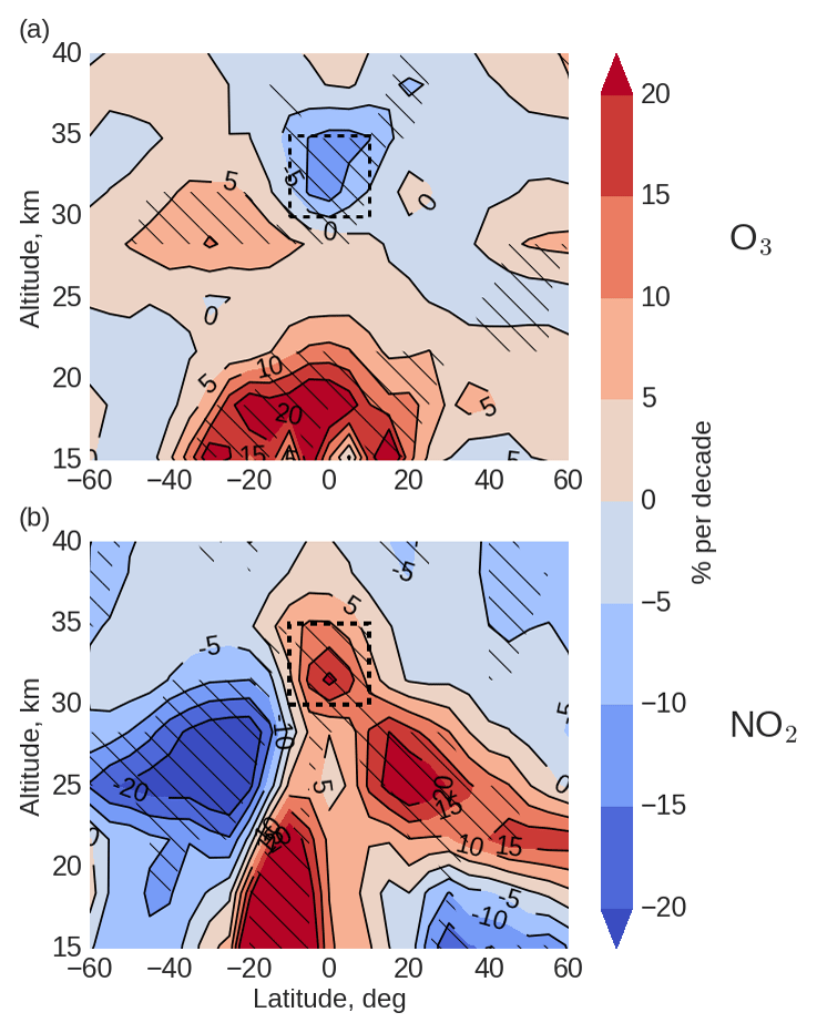
Figure 2Latitude–altitude distribution of (a) O3 and (b) NO2 changes (% decade−1) from MLR applied to SCIAMACHY measurements for the January 2004–April 2012 period. Hatched areas show changes significant at the 2σ level. The dashed rectangle indicates the region of the tropical mid-stratosphere investigated in this paper.
To identify possible reasons for the O3 changes in the tropical mid-stratosphere, and to check the role of N2O and NOx chemistry in these changes following suggestions by Nedoluha et al. (2015b), we analyse data from three TOMCAT simulations (see Sect. 2.2). Figure 3 presents latitude–altitude plots of the linear changes in O3 (panels a–c), NO2 (panels d–f), and N2O (panels g–i) for the period January 2004–April 2012 from TOMCAT (1) control run, CNTL – left column; (2) run with constant tropospheric mixing ratios of source gases, fSG – middle column; and (3) run with annually repeating meteorology, fDYN – right column. Results are shown on the native TOMCAT vertical grid. Latitude–altitude plots of equivalent NOx and NOy linear changes from TOMCAT are shown in Figs. S1–S2 of the Supplement. The CNTL simulation shows negative O3 changes in the tropical mid-stratosphere (Fig. 3a) of around 5 % decade−1 and positive NO2 changes (Fig. 3d) of around 10 % decade−1, which are similar, but somewhat smaller, than changes observed by SCIAMACHY (Fig. 2a, b). Figure 3g indicates a statistically significant N2O decrease of around 15 % decade−1 in the tropical mid-stratosphere and a pronounced hemispheric asymmetry with positive changes at southern and negative changes at northern mid-latitudes. These changes agree well with N2O trends from MLS during 2004–2013 (see Nedoluha et al., 2015a, Fig. 10). Such variations in N2O, a long-lived tracer with the global lifetime of around 115–120 years (Portmann et al., 2012), might indicate possible changes in the deep branch of the BDC.
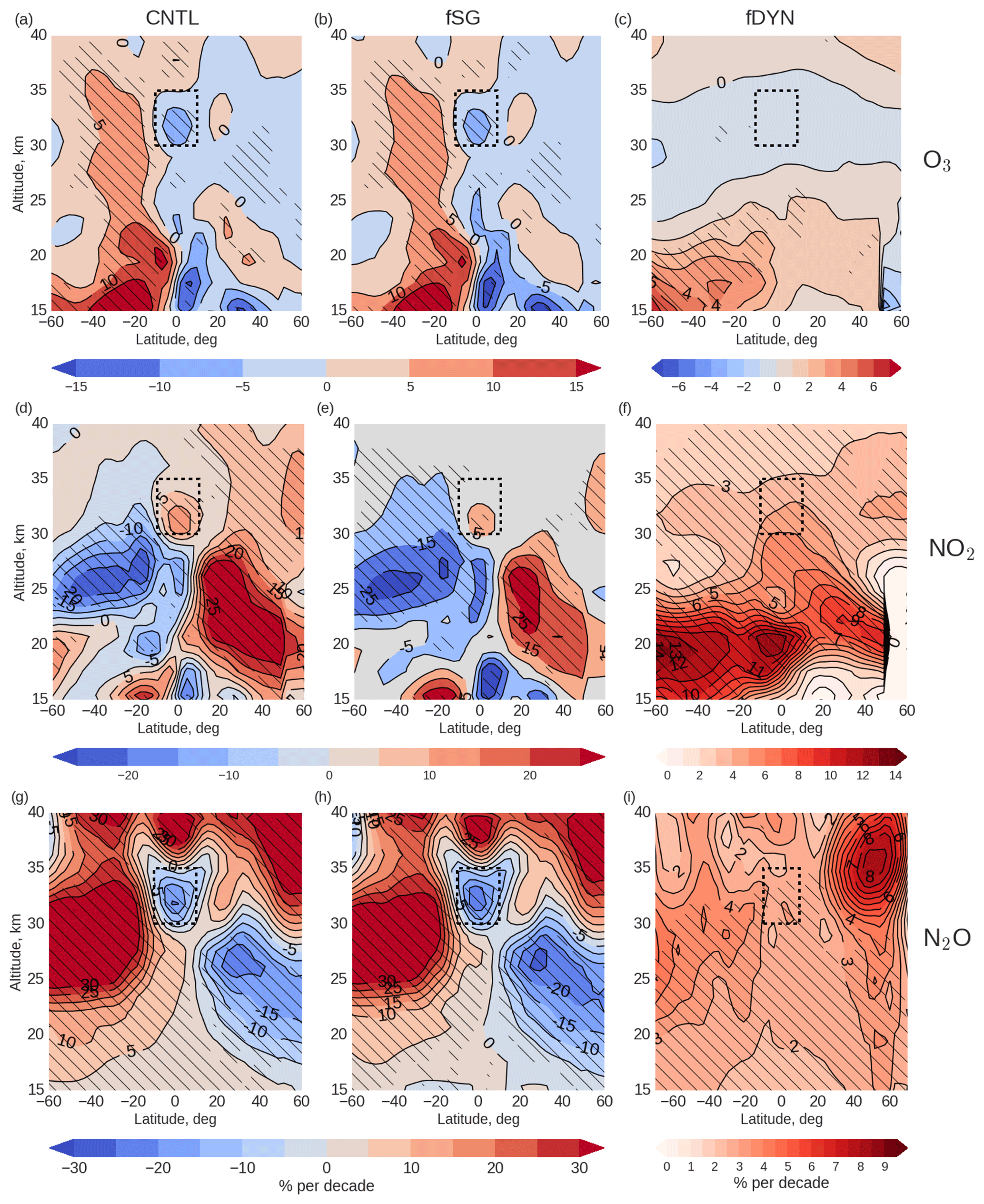
Figure 3Latitude–altitude distribution of (a–c) O3, (d–f) NO2, and (g–i) N2O changes (% decade−1) from the MLR model applied to TOMCAT runs in the January 2004–April 2012 period: CNTL (a, d, g), fSG (b, e, h), and fDYN (c, f, i). Latitude ranges from 60∘ S to 60∘ N, and altitude ranges from 15 to 40 km. Hatched areas show changes significant at the 2σ level. The dashed rectangle indicates the region of interest in this paper.
To distinguish the role of transport for O3, NO2, and N2O changes in the tropical mid-stratosphere, we show the results of the TOMCAT fSG simulation with constant tropospheric mixing ratios of all source gases in the middle column of Fig. 3. The modelled changes from both runs CNTL and fSG are very similar for O3 (Fig. 3a, b), NO2 (Fig. 3d, e), and N2O (Fig. 3g, h). This illustrates that the observed changes in the tropical mid-stratosphere are mostly of dynamical origin. The TOMCAT fDYN simulation, with annually repeating meteorology, shows insignificant (slightly negative) changes in O3 (Fig. 3c). Both NO2 (Fig. 3f) and N2O (Fig. 3i) show statistically significant but very weak positive changes in the tropical mid-stratosphere of around 3 % decade−1. This indicates that the direct impact of the chemistry on observed variations in O3, NO2, and N2O is rather small.
3.2 Tropical mid-stratospheric correlations
A powerful diagnostic for identifying the impact of chemical and dynamical processes on specific stratospheric constituents are tracer–tracer correlation plots (e.g. Sankey and Shepherd, 2003; Hegglin and Shepherd, 2007). Figure 4 shows correlation plots of N2O versus NO2 and N2O versus O3 in the tropical mid-stratosphere from the TOMCAT run CNTL. The colour coding classifies data according to altitude: 31 km (orange), 32 km (magenta), 33.5 km (sky blue), and 35 km (green). The panels show monthly mean data over the period January 2004–April 2012. Due to its long lifetime, N2O values reflect transport patterns: low N2O values indicate older air and high N2O values younger air. Figure 4a shows the N2O–NO2 anti-correlation that results from N2O chemical loss, which produces NO2 and is thus coupled to dynamical changes. Namely, when the upwelling is accelerated, more N2O is transported from lower altitudes, but less NO2 (and therefore NOy) is formed as the residence time of N2O decreases. Consequently, there is less time to produce NO2 via Reaction (R8a). In contrast, with slower upwelling less N2O is transported to the mid-stratosphere, but its residence time is longer, which allows for increased NO2 production. Figure 4a, clearly shows the larger abundance of N2O observed at 31 km (160–200 ppbV) than at 35 km (50–140 ppbV). This indicates the time needed to transport air masses between the two altitudes, which in turn favours larger NO2 production at 35 km of around 4.5–5.5 ppbV in comparison to 3–4.5 ppbV at 31 km. NO2 produced from the oxidation of N2O impacts O3. Figure 4b shows the N2O and O3 correlation. There is a linear relation, as the lifetime of both tracers in this region is greater than their vertical transport timescales (Bönisch et al., 2011). Both panels of Fig. 4 show quite compact correlations between the tracers, which indicate well mixed air masses (Hegglin et al., 2006).
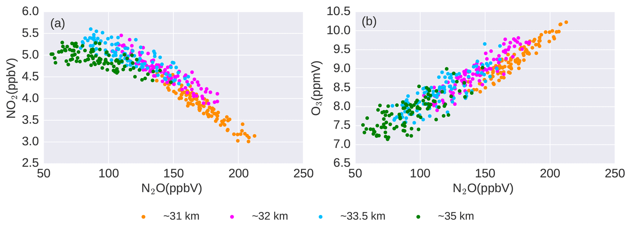
Figure 4Scatter plots of monthly mean (a) N2O versus NO2 and (b) N2O versus O3 in the tropical mid-stratosphere during January 2004–April 2012 from TOMCAT simulation CNTL. Colour coding classifies data according to altitude: 31 km (orange), 32 km (magenta), 33.5 km (sky blue), and 35 km (green).
To obtain more detailed information about tracer distributions, in particular on the NO2 impact on the observed negative O3 change, we present NO2–O3 scatter plots at 31.5 km in the tropics in Fig. 5 from SCIAMACHY measurements and TOMCAT simulations CNTL, fSG, and fDYN. Data points indicate zonal monthly mean values during January 2004–April 2012. Here TOMCAT results are interpolated to the SCIAMACHY vertical grid. Solid lines in each panel specify linear fits to corresponding data points and represent the chemical link between O3 and NO2. All panels of Fig. 5 show the expected negative correlation of O3 with NO2. The SCIAMACHY NO2–O3 distribution (Fig. 5a) agrees well with the TOMCAT CNTL simulation (Fig. 5b), although modelled NO2 and O3 are lower in comparison with measurements.
To further investigate the impact of dynamics on NO2–O3 changes, Fig. 5c shows a combined scatter plot from both simulations (CNTL and fSG). In conditions of unchanged tropospheric mixing ratios of source gases (fSG, orange points), the data scatter and slopes do not change significantly in comparison with the control simulation (CNTL, green points). Both simulations are performed with the same dynamical forcing. In contrast, the NO2–O3 scatter from CNTL and fDYN TOMCAT simulations (Fig. 5d) differ significantly. In the absence of dynamical changes (red points) the NO2 and O3 scatter plots do not show such large variability as in run CNTL (green points), which highlights the impact of transport and indicates different tracer distributions with and without dynamical changes. However, the slopes are similar in both simulations, which represents the chemical impact of NOx changes on O3. Therefore, the NO2–O3 scatter plots from the model calculations confirm the notion that observed O3 changes are linked to NOx chemistry in the tropical mid-stratosphere. Also, it follows from the different TOMCAT simulations that these chemical changes on shorter timescales are ultimately driven by dynamical variations.

Figure 5NO2–O3 scatter plots in the tropical stratosphere at an altitude of 31.5 km from (a) SCIAMACHY and TOMCAT simulations (b) CNTL, (c) CNTL and fSG, and (d) CNTL and fDYN. Colour coding denotes data source: SCIAMACHY (dark blue), TOMCAT: CNTL (green), fSG (orange), and fDYN (red). Solid lines specify linear fits to the data points.
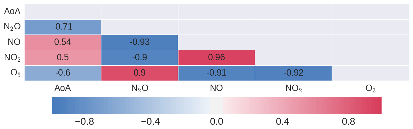
Figure 6Correlation heat map for monthly means of AoA, N2O, NO, NO2, and O3 from TOMCAT CNTL run for the period January 2004–April 2012 in the tropical mid-stratosphere. Repeated information was excluded from the heat map.
Recognizing the tight relationships within the tropical mid-stratosphere N2O–NOx–O3 chemistry, seen in Figs. 4 and 5, we calculated Pearson correlation coefficients between the chemical species as well as with the dynamical AoA tracer. Figure 6 shows the correlation heat map for AoA, N2O, NO, NO2, and O3 for the period January 2004–April 2012 in this region. The correlations between the monthly means of the chemical species N2O, NO, NO2, and O3 are very high and in all cases exceed 0.9, which is consistent with the tracer–tracer correlations shown in Figs. 4a, b and 5a–d. The overall high correlation as shown in the heat map can be explained by the overall regulation of the O3 abundance in the tropical mid-stratosphere. Ozone is mainly destroyed by NOx in this altitude region and the strong chemical link between O3 and NOx is confirmed by the high anti-correlation (0.92). A strong anti-correlation is expected between N2O and NOy as these are both long-lived tracers in the mid-lower stratosphere and N2O is the source of NOy. As the amount of NOx also scales with the amount of NOy, a fairly strong correlation (0.9) exists between N2O and O3, even in the mid-stratosphere where the O3 photochemical lifetime becomes short.
The correlation of AoA with all tracers is rather moderate (with absolute values within the range of 0.5–0.71), as transport (or AoA) does not directly control NO, NO2, or O3 in this region. The anti-correlation of N2O and AoA is also moderate (−0.71), which is unexpected as the major source of N2O in the tropical mid-stratosphere is the upwelling from lower altitudes (see Sect. 1).
3.3 N2O – age of air relationship
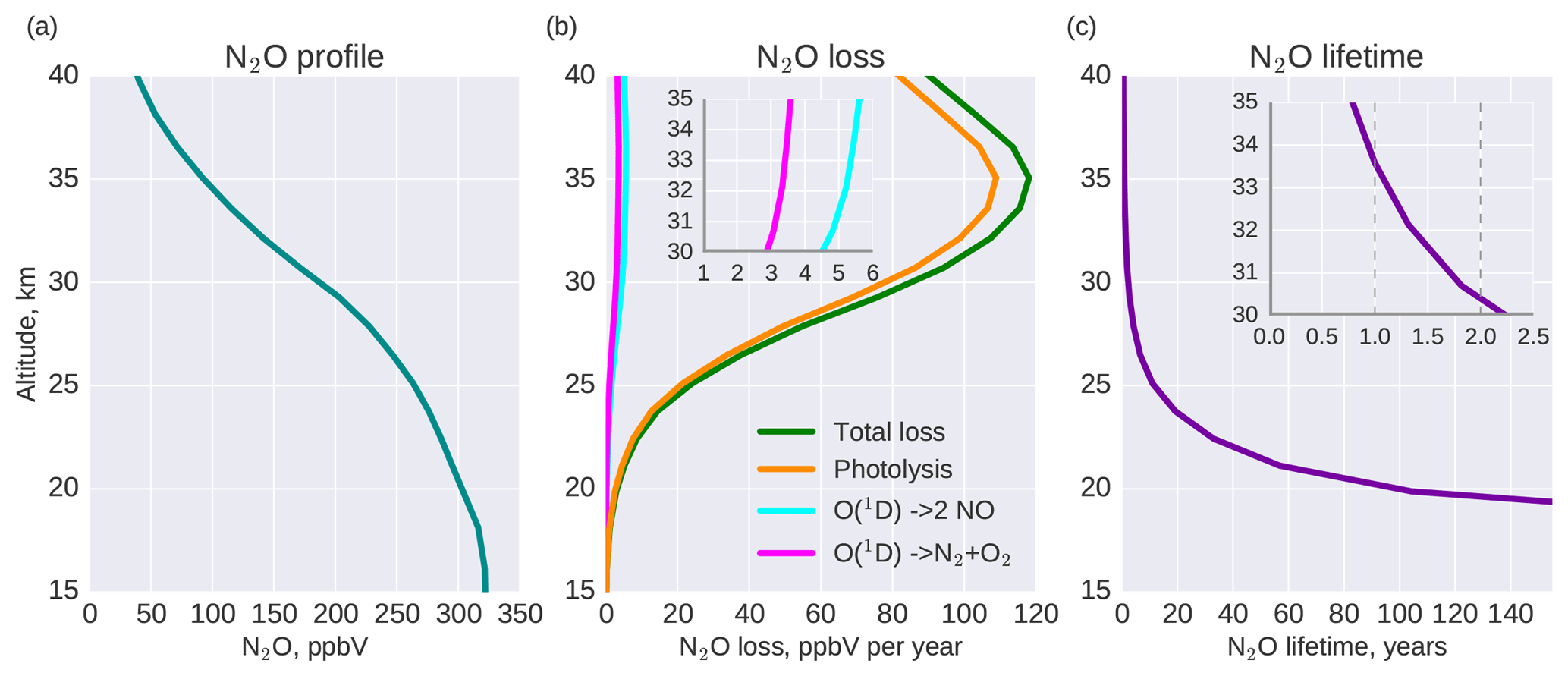
Figure 7Average profiles of (a) N2O (ppbV), (b) N2O loss (ppbV year−1), and (c) N2O lifetime (years) from TOMCAT for the period 2004–2012. Colour coding in panel (b) indicates the source of N2O loss: total loss – green; loss via photolysis Reaction (R7) – orange; loss via oxidation with NOx production Reaction (R8a) – turquoise; loss via oxidation without NOx production Reaction (R8b) – magenta.
To improve our understanding of the AoA–N2O relation, Fig. 7 shows profiles of N2O, N2O loss, and N2O lifetime from the TOMCAT CNTL run, averaged over the period 2004–2012. A significant decrease in N2O concentrations with altitude is seen in Fig. 7a, in particular a sharp decrease around 20 km altitude. Figure 7b shows that the largest (∼ 90 %) N2O loss is caused by photolysis Reaction (R7, orange), which starts to become important at around 20 km altitude. About 5–10 % of N2O reacts with O(1D) above 26 km, where the concentration of O(1D) starts slowly increasing due to the Reaction (R3a). As the consequence of these N2O loss reactions, its average lifetime (shown in Fig. 7c), calculated as the ratio of mean N2O concentration and its total loss is also strongly altitude dependent. It varies from more than 100 years at 20 km to less than 1 year at 35 km. In particular, in the altitude range 30–35 km the N2O lifetime varies by a factor of 2 (Fig. 7c).
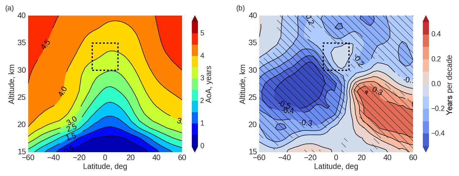
Figure 8Latitude–altitude AoA (a) the zonally averaged distribution (years), (b) the linear changes (years decade−1) from the MLR model applied to the TOMCAT CNTL simulation during January 2004–April 2012: latitude range is from 60∘ S to 60∘ N, altitude range is from 15 to 40 km. The dashed rectangle indicates the region of interest in the tropical mid-stratosphere. The hatched areas in (b) show changes significant at the 2σ level.
To investigate the link between transport and N2O, we show zonally averaged climatological mean AoA (years, in Fig. 8a) and AoA linear changes (years decade−1, Fig. 8b) as a function of latitude and altitude from the TOMCAT CNTL simulation during January 2004–April 2012. The dashed rectangle indicates the region of interest. Hatched areas in Fig. 8b show regions where changes are significant at the 2σ level. According to Fig. 8a the average lifetime of air is around 3.5 years in the tropical mid-stratosphere, and according to Fig. 8b there are no statistically significant changes in AoA in the same region. The absence of statistically significant AoA changes here is, on the one hand, in agreement with Aschmann et al. (2014) who demonstrated that the deep branch of BDC does not show significant changes. On the other hand, it is apparently inconsistent with (1) N2O negative changes identified in the region of interest (Fig. 3g) and (2) conclusions of Nedoluha et al. (2015b) who suggested a decrease in upwelling speed as a possible reason for the observed O3 decline at 10 hPa (around 30–35 km altitude).
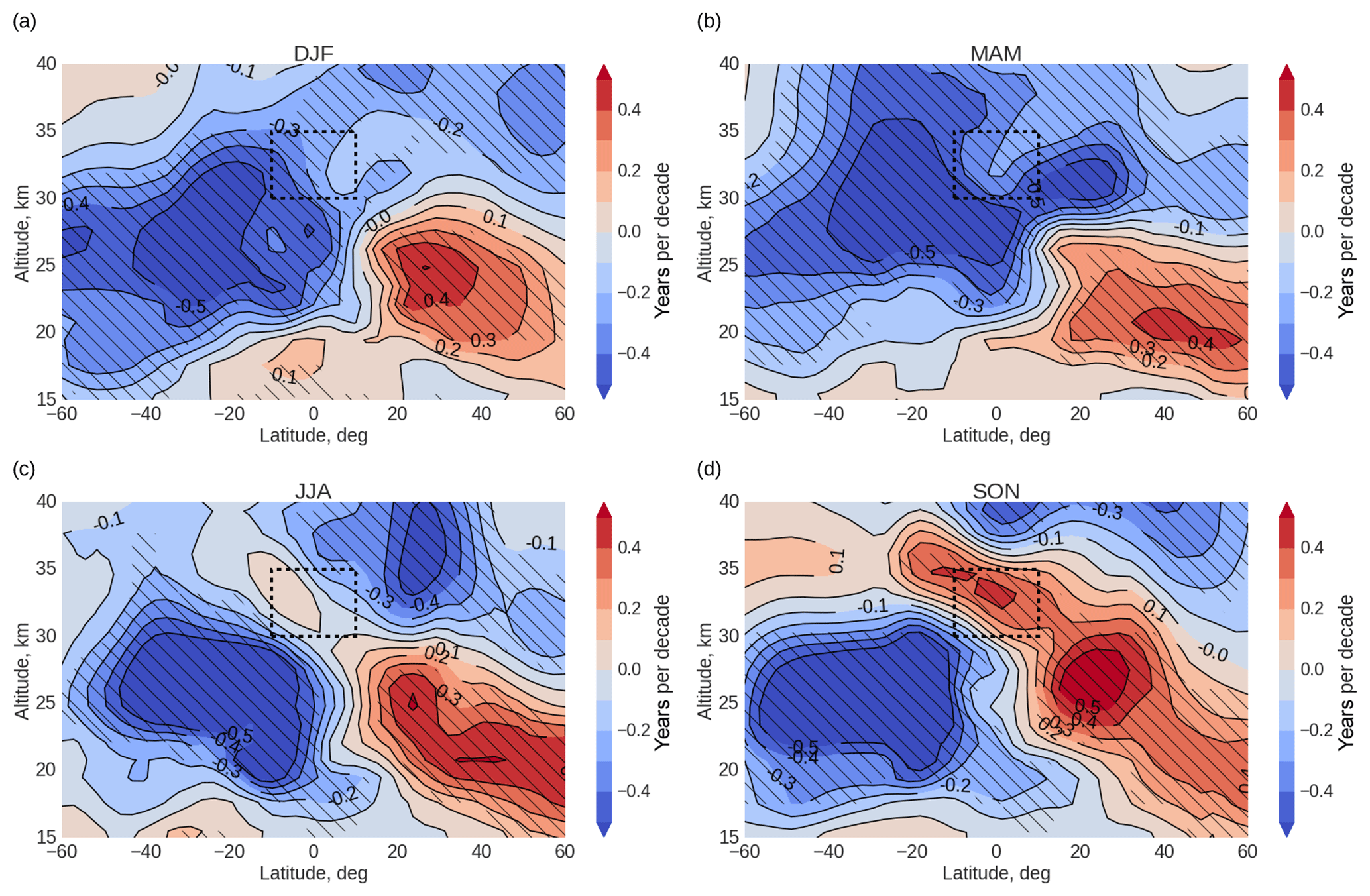
Figure 9Latitude–altitude distribution of AoA changes (years decade−1) from MLR model based on the TOMCAT CNTL simulation during January 2004–April 2012 for (a) DJF, (b) MAM, (c) JJA, (d) SON: latitude range from 60∘ S to 60∘ N, altitude range from 15 to 40 km. Hatched areas show changes significant at the 2σ level. The dashed rectangle indicates the region of the tropical mid-stratosphere investigated in this paper.
To further improve our understanding of AoA changes, we show in Fig. 9 a seasonal analysis of AoA linear changes (years decade−1) from the MLR model during January 2004–April 2012 based on TOMCAT CNTL simulation for DJF (panel a), March–April–May (MAM, panel b), June–July–August (JJA, panel c), and September–October–November (SON, panel d). Figure 9 shows that in the tropical mid-stratosphere, AoA changes vary significantly during seasons: AoA decreases during DJF and MAM (Fig. 9a, b) and increases during SON (Fig. 9d). During JJA (Fig. 9c) no statistically significant changes in AoA in tropical mid-stratosphere were identified. The seasonality in AoA changes in the tropical mid-stratosphere leads to insignificant changes when averaged over the entire year (seen in Fig. 8b). Another interesting pattern shown in Fig. 8b is the clear asymmetry between the hemispheres, with negative AoA changes in the southern and positive AoA changes in the northern hemispheres. This asymmetry is consistent with the results presented in Sect. 3.1 for N2O changes (Fig. 3g, h) and in agreement with Mahieu et al. (2014) and Haenel et al. (2015). The hemispheric asymmetry, however, remains unchanged within all seasons (Fig. 9a–c).
From the above, the major resulting question is the following. How are N2O and transport (via AoA) connected? To answer this, we analyse N2O–AoA correlation coefficients as a function of month (Fig. 10) at altitudes of 32, 33, and 35 km. To overcome any hemispheric dependencies, we split the tropics into southern (10–1∘ S) and northern (1–10∘ N) regions. Correlation coefficients were calculated on the native TOMCAT grid. Horizontal dashed lines indicate an arbitrary threshold of moderate correlation, which is represented by the value of −0.6.

Figure 10N2O–AoA anti-correlation as a function of month averaged for the period January 2004–April 2012 for (a) 10∘ S–10∘ N, (b) 10–1∘ S, and (c) 1–10∘ N. Colour coding indicates altitude: 32 km (orange), 33 km (magenta), and 35 km (cyan). The dashed horizontal lines indicate an arbitrary threshold of moderate correlation, which was selected to be the value of −0.6.
Figure 10a shows that in the tropical region (10∘ S–10∘ N) the AoA–N2O anti-correlation is very low during December–March. During the other months of the year, it is moderate and reaches maximum values (around 0.9) during late Northern Hemisphere summer (August) and autumn (September, October) months. Very similar seasonal behaviour is also observed in the tropical region of the Southern Hemisphere (Fig. 10b) with the minimum correlation occurring during December–March (Southern Hemisphere summer) and maximum during May–October (Southern Hemisphere winter). In contrast, in the tropical region of the Northern Hemisphere (Fig. 10c) a significant decrease in AoA–N2O anti-correlation is observed during summer months (June–July). Similar seasonal variations in N2O–AoA anti-correlation are observed in narrower latitude bands (4∘ S–4∘ N), which are shown in Fig. S3. The common characteristic of seasonal changes in AoA–N2O is that a significant decrease in the anti-correlation is observed during local summer in each hemisphere. This is the period when the strength of the BDC is the lowest (Kodama et al., 2007, and references therein) and no significant changes in AoA are observed. The overall correlation for inner tropics from 10∘ S to 10∘ N, as shown in Fig. 10a, combines the behaviour of both hemispheres.
With knowledge of the existence of strong seasonal dependencies in AoA variability, and therefore in N2O, we have analysed the AoA–N2O relation as a function of month, averaged for the period January 2004–April 2012. Figure 11 shows N2O mixing ratio and AoA averaged over January 2004–April 2012 as a function of month and altitude. The matching of the colour and contour isolines is pronounced, confirming a direct link between N2O and AoA. Furthermore, as N2O is transported from the troposphere, its concentrations decrease with altitude (see also Sect. 1). In the lower stratosphere (15–20 km) the seasonal variations in N2O and AoA exist, but are not as pronounced as in the mid-stratosphere (30–35 km). Moreover, the seasonal variations in N2O are larger than the seasonal variations in AoA, so the correlation breaks down (as seen from Fig. 8). There are two distinct seasonal features seen in the N2O–AoA distribution in the mid-stratosphere, which increase at a given altitude during January–March and September–November. During these periods, AoA becomes lower in comparison with the rest of the year (indicating younger air) and therefore more N2O is transported to these altitudes.
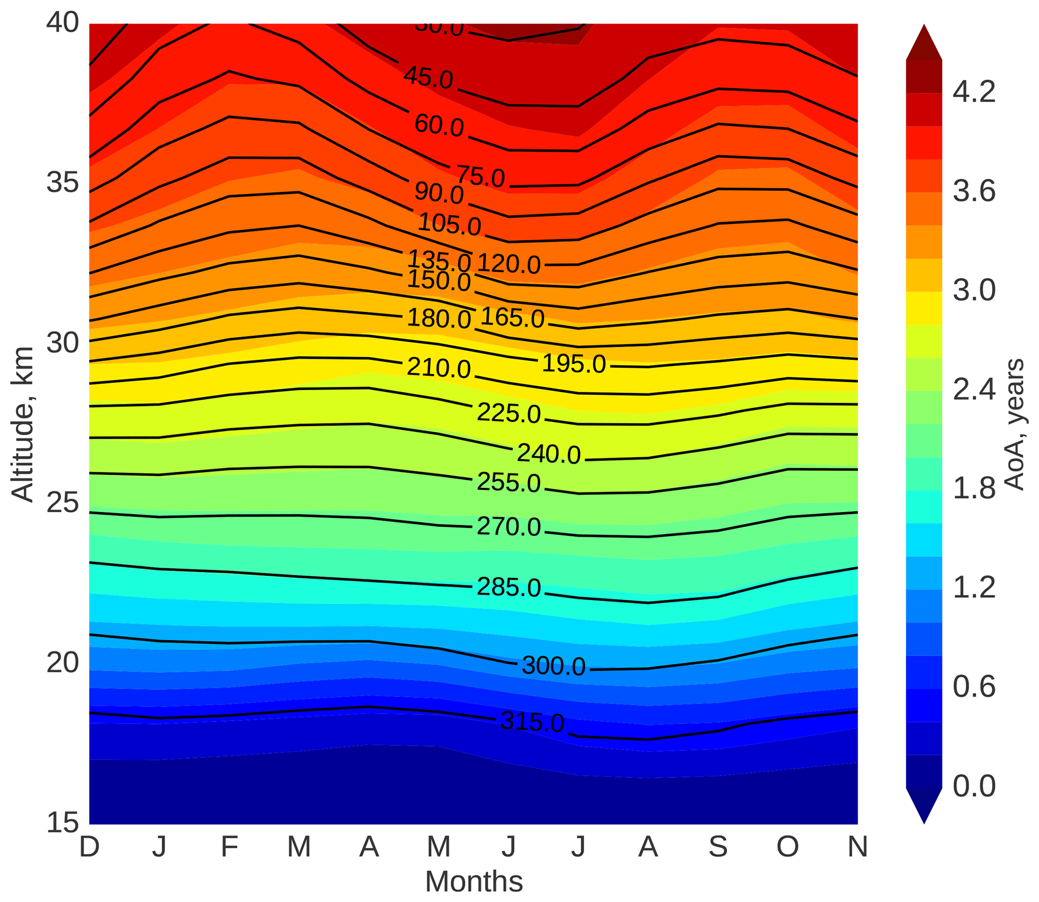
Figure 11Annual cycle of monthly mean N2O (ppbV, contours, 15 ppbV interval) and AoA (years, colours, 0.2-year interval) as a function of altitude from TOMCAT run CNTL in the tropical region, averaged over the period January 2004–April 2012.
3.4 Observed changes in the tropical mid-stratosphere
Figures 10 and 11 show the seasonal variations in AoA and N2O in the tropical mid-stratosphere. To further investigate the possible chemical impact on other species, we analysed linear changes in AoA, N2O, NO2, and O3 from TOMCAT run CNTL and SCIAMACHY measurements for each calendar month (see Figs. S4–S7). TOMCAT run CNTL in general shows lower O3 and NO2 concentrations compared to SCIAMACHY measurements as discussed earlier. The underestimation of modelled NO2 and O3 is also evident when comparing Fig. 5a and b, but the slope of the modelled anti-correlation regression line agrees very well with that of the SCIAMACHY observations. The reason for these biases between model and measurements is not clear. However, if the model NO2 increases then O3 will decrease even further (Fig. 5). Therefore, it is unlikely that transport errors are the cause. Either the model underestimates the production of O3 from O2 photolysis in this region, or there are uncertainties in the model NOx chemistry, which means the impact of NO2 on O3 is less than modelled. The latter uncertainties would then be associated with the reactions , or NO2 photolysis.
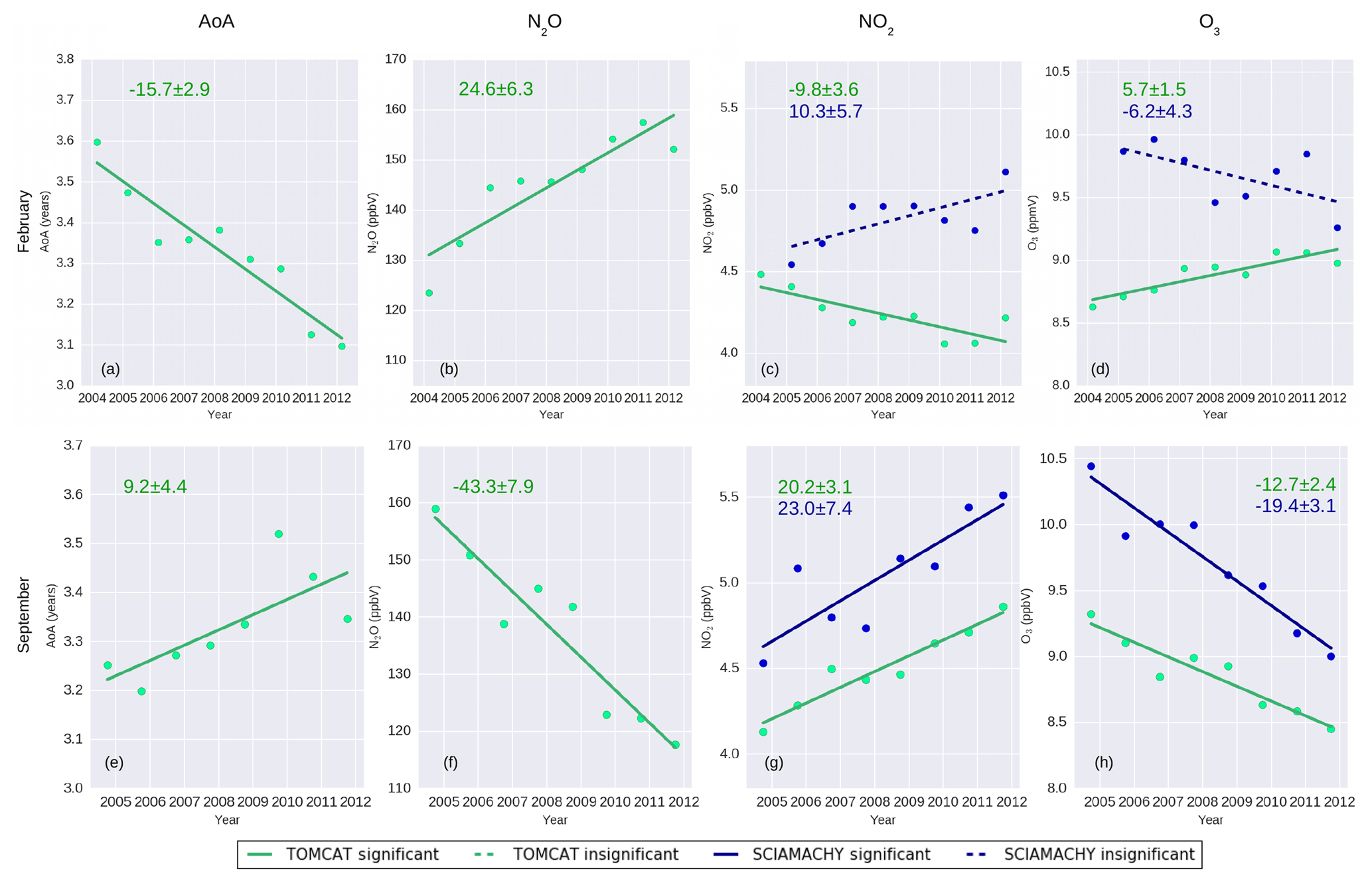
Figure 12Linear changes in AoA, N2O, NO2, and O3 minus QBO effect averaged over (a–d) Februaries 2004–2012 and (e–h) Septembers 2004–2011 in the tropical stratosphere between 30 and 35 km altitude. Colour coding indicates the data source: TOMCAT CNTL simulation (green) and SCIAMACHY measurements (dark blue). Colour-coded trend values and their errors (in % decade−1) are shown in each panel. Solid lines indicate statistically significant linear changes at the 2σ level, dashed lines indicate statistically insignificant changes.
The upper panels of Fig. 12 show linear changes in February AoA, N2O, NO2, and O3 from TOMCAT CNTL run (green) and SCIAMACHY measurements (dark blue). Solid lines in Fig. 12 indicate statistically significant linear changes (2σ), while dashed lines indicate statistically insignificant gradients or linear changes. The TOMCAT results yield a February decrease in AoA with time and a small O3 recovery. Similar results from TOMCAT are calculated for January (Fig. S4). In particular, the faster upwelling as indicated by the decrease in AoA (Fig. 12a) results in more intense N2O transport. Consequently, N2O increases with time (Fig. 12b) while NO2 decreases (Fig. 12c) due to the shorter residence time of N2O, i.e. there is less time to produce NOx species via the O(1D) Reaction (R8a). Finally, a small increase in O3 is observed in the tropical mid-stratosphere (Fig. 12d). SCIAMACHY measurements show statistically insignificant changes in NO2 and O3 during Januaries and Februaries (Figs. 12c, d, S4). Contrary to the TOMCAT simulations, SCIAMACHY measurements do not show any statistically significant NO2 decrease or O3 increase when analysing changes for any particular calendar month. From September to February, the gradient of O3 time series increases, becoming more positive for both SCIAMACHY and TOMCAT data, resulting for February in small statistically insignificant negative gradients for SCIAMACHY observations and small but statistically significant positive gradients for TOMCAT. Similarly for NO2 mixing ratios, from September to February the gradients decrease, i.e. they become more positive for both SCIAMACHY and TOMCAT results. The SCIAMACHY data show larger errors in gradients of the time series for individual months, than those of the TOMCAT model. This results from the stronger oscillating structure in the SCIAMACHY time series. The reasons for the observed oscillations and their strength are not yet unambiguously identified and are under investigation.
The lower panels of Fig. 12 show the changes in September AoA, N2O, NO2, and O3. The linear change or gradients are opposite to those of the winter months shown in the upper panels. October shows a similar behaviour to that of September (see Fig. S7). Positive AoA changes (Fig. 12e) indicate a significant transport slowdown or additional mixing of air. As a result, there is less N2O transported from the troposphere (Fig. 12f) and consequently more N2O is photolytically destroyed. The residence time in the tropical mid-stratosphere becomes longer, producing more NO2 (Fig. 12g) which leads to more effective O3 destruction (Fig. 12h). SCIAMACHY NO2 and O3 changes agree well with the model results in September and October (Figs. 12g, h and S7).
The negative AoA gradients for the 2004–2012 period during the boreal winter months (January and February) and positive AoA gradients during the boreal autumn months (September and October) cancel, i.e. there is no statistically significant linear change or gradient in the annual mean AoA (Fig. 8b). In contrast, the monthly gradients over the same periods for the chemical species N2O; NO2; and, as a result of the NOx ozone catalytic destruction cycle, O3 do not cancel in the annual means. This effect is primarily attributed to the non-linear relationship between AoA and N2O. That implies that, for example, the slowdown in tropical upwelling would indicate (1) slower N2O transport from lower altitudes, which would lead to a decrease in N2O, and (2) destruction of more N2O by photolysis (Reaction R7, around 90 %) and O1D (Reactions R8a and R8b, around 10 %), as the residence time of N2O in this region becomes longer. In contrast, the speed-up in tropical upwelling would mean that more N2O is transported from the lower altitudes, and its residence time is shorter. This leads to lower N2O destruction via photochemistry. The amounts of NO2 and O3 are chemically linked to that of N2O. Overall, the changes in NO2 and O3 are dependent on both the amount of N2O transported to the stratosphere and its residence time.
We have analysed O3 changes in the tropical mid-stratosphere during January 2004–April 2012 as observed by SCIAMACHY and simulated by the TOMCAT CTM. We find that the model, forced by ECMWF reanalyses, captures well the observed linear O3 changes within the analysed period. Using a set of TOMCAT simulations with different dynamical and chemical forcings we showed that the decline in O3 is ultimately dynamically controlled and occurs due to increases in NO2, which then chemically removes O3. The NO2 increases are due to a longer residence time of its main source N2O, which is long-lived so changes in its abundance indicate variations in the tropical upwelling. These results are in agreement with findings of Nedoluha et al. (2015b). To further investigate whether there was a decrease in tropical upwelling we analysed the AoA from the TOMCAT model. However, the AoA simulations did not show any significant annual mean changes in the tropical mid-stratosphere, in apparent contradiction with conclusions from Nedoluha et al. (2015b).
With the knowledge of dynamically driven N2O–NO2–O3 changes but no significant changes in mean AoA, we performed a detailed analysis of linear changes for each month separately within the period January 2004–April 2012. We find that during boreal autumn months, i.e. September and October in the north, there is a significant transport slowdown or additional air mixing that corresponds to positive changes in AoA. These positive changes cause longer residence time of N2O, leading to increased NOx production and stronger O3 loss. SCIAMACHY and TOMCAT O3 and NO2 changes are consistent in that regard. In contrast, we find that during boreal winter months, i.e. January and February, the AoA simulations show a transport speed-up. This decreases the residence time of N2O, so less NOx is produced and consequently less O3 is destroyed. While the TOMCAT model shows significant NOx decrease and O3 increase, the SCIAMACHY changes are not significant during these winter months. This is associated with larger uncertainties in the MLR applied to the satellite data.
Starting from the seasonal variation in AoA changes and its impact on annual mean trends in the tropical mid-stratosphere as presented in this paper, some questions still remain and should be the subject of further studies. Is the shift of subtropical transport barriers, as suggested by Eckert et al. (2014) and Stiller et al. (2017), linked to the seasonal AoA changes observed here? Or is this a result of the different behaviour of the shallow and deep branches of the BDC, i.e. hiatus in the acceleration of the shallow branch, strengthening of the transition branch, and no significant changes in the deep branch (Aschmann et al., 2014)? The cooling in the eastern Pacific (Meehl et al., 2011) could also affect O3 changes via upwelling, although our analysis of sea surface temperatures (not shown here) did not show significant monthly variations. Another plausible explanation of changes in the transport regime could be from planetary wave forcing (Chen and Sun, 2011), as we find that a significant decrease in the N2O–AoA correlations occurs during local summers, when the wave activity and therefore the strength of the upwelling is the lowest. In particular, the impact of variations in the wave activity on seasonal build up of O3 was also described by Shepherd (2007). However, all of these possible explanations require additional investigation to decide which processes dominate.
Overall, the non-linear relation of AoA and N2O and their month-to-month changes presented in this paper explain well the observed O3 decline in the tropical mid-stratosphere. With the application of a detailed CTM, we are able not only to confirm the O3 decline but also describe chemical impacts and define the role of dynamics on the observed changes. Having identified the impact of a seasonal dependency of the upwelling speed on tropical mid-stratospheric O3 in this study, a better understanding of the possible drivers of this behaviour is now required. However, the CTM with its specified meteorology cannot be used to determine the main drivers of the dynamical changes. Consequently, the application of interactive dynamical models is needed. The interpretation of the observed changes will give us an understanding of whether O3 decline in the tropical mid-stratosphere is part of natural variability, human impact, or a complex interaction of both factors.
SCIAMACHY O3 and NO2 data are available after registration at http://www.iup.uni-bremen.de/scia-arc/ (Rozanov, 2019). Results of TOMCAT simulations are available upon request from the authors. QBO equatorial winds at 10 and 30 hPa were taken from http://www.geo.fu-berlin.de/en/met/ag/strat/produkte/qbo/index.html (Kunze et al., 2019). The anomalies of the Nino 3.4 index were downloaded from http://www.cpc.ncep.noaa.gov/data/indices/ (NOAA, 2019). Data of the Mg II index from GOME, SCIAMACHY, and GOME-2 were taken from http://www.iup.uni-bremen.de/UVSAT/Datasets/mgii (Weber et al., 2019).
The supplement related to this article is available online at: https://doi.org/10.5194/acp-19-767-2019-supplement.
EG performed the trend analyses, was the lead author of the manuscript, and prepared the figures. All co-authors commented on the initial and revised drafts of the manuscripts. AR supervised and guided the computation of the trends, provided SCIAMACHY datasets, and expertise on data usage. MPC and SSD designed and performed the TOMCAT runs, contributed to the data analysis, and scientific interpretation of the results. MW contributed to the trend analysis and the scientific interpretation of the results. CA provided help with trend analysis. WF provided support for the TOMCAT simulations. JPB initiated and coordinated the study, contributed to the data analysis, the scientific outcomes, and preparation of the manuscript.
The authors declare that they have no conflict of interest.
This research has been partly funded by the University and State of Bremen,
by the Postgraduate International Programme in Physics and Electrical
Engineering (PIP) of the University of Bremen, by the project SHARP-II-OCF,
and by a “BremenIDEA out” scholarship, promoted by the German Academic
Exchange Service (DAAD) and funded by the Federal Ministry of Education and
Research (BMBF). This research is also in part a preparatory contribution to
the German BMBF ROMIC II project and the DFG VolImpact Research
Unit. The model simulations were performed on the UK national Archer and
Leeds ARC HPC facilities. MPC is supported by a Royal Society Wolfson Merit
Award. The authors thank Amanda Maycock and Andreas Chrysanthou for comments
on early stages of this research. The data presented were partially obtained
using the German High Performance Computer Center North (HLRN) service, whose
support is gratefully acknowledged.
Edited by:
Martin Dameris
Reviewed by: two anonymous referees
Arfeuille, F., Luo, B. P., Heckendorn, P., Weisenstein, D., Sheng, J. X., Rozanov, E., Schraner, M., Brönnimann, S., Thomason, L. W., and Peter, T.: Modeling the stratospheric warming following the Mt. Pinatubo eruption: uncertainties in aerosol extinctions, Atmos. Chem. Phys., 13, 11221–11234, https://doi.org/10.5194/acp-13-11221-2013, 2013. a
Aschmann, J., Burrows, J. P., Gebhardt, C., Rozanov, A., Hommel, R., Weber, M., and Thompson, A. M.: On the hiatus in the acceleration of tropical upwelling since the beginning of the 21st century, Atmos. Chem. Phys., 14, 12803–12814, https://doi.org/10.5194/acp-14-12803-2014, 2014. a, b, c, d
Ball, W. T., Alsing, J., Mortlock, D. J., Staehelin, J., Haigh, J. D., Peter, T., Tummon, F., Stübi, R., Stenke, A., Anderson, J., Bourassa, A., Davis, S. M., Degenstein, D., Frith, S., Froidevaux, L., Roth, C., Sofieva, V., Wang, R., Wild, J., Yu, P., Ziemke, J. R., and Rozanov, E. V.: Evidence for a continuous decline in lower stratospheric ozone offsetting ozone layer recovery, Atmos. Chem. Phys., 18, 1379–1394, https://doi.org/10.5194/acp-18-1379-2018, 2018. a
Bönisch, H., Engel, A., Birner, Th., Hoor, P., Tarasick, D. W., and Ray, E. A.: On the structural changes in the Brewer-Dobson circulation after 2000, Atmos. Chem. Phys., 11, 3937–3948, https://doi.org/10.5194/acp-11-3937-2011, 2011. a
Bovensmann, H., Burrows, J. P., Buchwitz, M., Frerick, J., Noël, S., Rozanov, V. V., Chance, K. V., and Goede, A. P. H.: SCIAMACHY: Mission Objectives and Measurement Modes, J. Atmos. Sci., 56, 127–150, 1999. a
Bregmann, A., Lelieveld, J., van den Broek, M. M. P., Siegmund, P. C., Fischer, H., and Bujok, O.: N2O and O3 relationship in the lowermost stratosphere: A diagnostic for mixing processes as represented by a three-dimensional chemistry-transport model, J. Geophys. Res.-Atmos., 105, 17279–17290, https://doi.org/10.1029/2000JD900035, 2000. a
Burrows, J. P., Hölzle, E., Goede, A., Visser, H., and Fricke, W.: SCIAMACHY – Scanning Imaging Absorption Spectrometer for Atmospheric Chartography, Acta Astron., 35, 445–451, https://doi.org/10.1016/0094-5765(94)00278-T, 1995. a
Butz, A., Bösch, H., Camy-Peyret, C., Chipperfield, M., Dorf, M., Dufour, G., Grunow, K., Jeseck, P., Kühl, S., Payan, S., Pepin, I., Pukite, J., Rozanov, A., von Savigny, C., Sioris, C., Wagner, T., Weidner, F., and Pfeilsticker, K.: Inter-comparison of stratospheric O3 and NO2 abundances retrieved from balloon borne direct sun observations and Envisat/SCIAMACHY limb measurements, Atmos. Chem. Phys., 6, 1293–1314, https://doi.org/10.5194/acp-6-1293-2006, 2006. a
Chapman, S. F.: On ozone and atomic oxygen in the upper atmosphere, The London, Edinburgh, and Dublin Philosophical Magazine and Journal of Science, 10, 369–383, https://doi.org/10.1080/14786443009461588, 1930. a
Chen, G. and Sun, L.: Mechanisms of the Tropical Upwelling Branch of the Brewer-Dobson Circulation: The Role of Extratropical Waves, J. Atmos. Sci., 68, 2878–2892, https://doi.org/10.1175/JAS-D-11-044.1, 2011. a
Chipperfield, M. P.: New version of the TOMCAT/SLIMCAT off-line chemical transport model: Intercomparison of stratospheric tracer experiments, Q. J. Roy. Meteor. Soc., 132, 1179–1203, https://doi.org/10.1256/qj.05.51, 2006. a
Chipperfield, M. P., Liang, Q., Strahan, S. E., Morgenstern, O., Dhomse, S. S., Abraham, N. L., Archibald, A. T., Bekki, S., Braesicke, P., Di Genova, G., Fleming, E. L., Hardiman, S. C., Iachetti, D., Jackman, C. H., Kinnison, D. E., Marchand, M., Pitari, G. A., Rozanov, P. J., Stenke, E. A., and Tummon, F.: Multimodel estimates of atmospheric lifetimes of long-lived ozone-depleting substances: Present and future, J. Geophys. Res.-Atmos., 119, 2555–2573, https://doi.org/10.1002/2013JD021097, 2014. a
Chipperfield, M. P., Bekki, S., Dhomse, S., Harris, N. R. P., Hassler, B., Hossaini, R., Steinbrecht, W., Thiéblemont, R., and Weber, M.: Detecting recovery of the stratospheric ozone layer, Nature, 549, 211–218, https://doi.org/10.1038/nature23681, 2017. a
Chipperfield, M. P., Dhomse, S., Hossaini, R., Feng, W., Santee, M. L., Weber, M., Burrows, J. P., Wild, J. D., Loyola, D., and Coldewey-Egbers, M.: On the Cause of Recent Variations in Lower Stratospheric Ozone, Geophys. Res. Lett., 45, L078071, https://doi.org/10.1029/2018GL078071, 2018. a
Coddington, O., Lean, J. L., Pilewskie, P., Snow, M., and Lindholm, D.: A Solar Irradiance Climate Data Record, B. Am. Meteorol. Soc., 97, 1265–1282, https://doi.org/10.1175/BAMS-D-14-00265.1, 2016. a
Crutzen, P. J.: The influence of nitrogen oxides on the atmospheric ozone content, Q. J. Roy. Meteor. Soc., 96, 320–325, https://doi.org/10.1002/qj.49709640815, 1970. a
Dee, D. P., Uppala, S. M., Simmons, A. J., Berrisford, P., Poli, P., Kobayashi, S., Andrae, U., Balmaseda, M. A., Balsamo, G., Bauer, P., Bechtold, P., Beljaars, A. C. M., van de Berg, L., Bidlot, J., Bormann, N., Delsol, C., Dragani, R., Fuentes, M., Geer, A. J., Haimberger, L., Healy, S. B., Hersbach, H., Hölm, E. V., Isaksen, L., Kållberg, P., Köhler, M., Matricardi, M., McNally, A. P., Monge-Sanz, B. M., Morcrette, J., Park, B., Peubey, C., de Rosnay, P., Tavolato, C., Thépaut, J., and Vitart, F.: The ERA-Interim reanalysis: configuration and performance of the data assimilation system, Q. J. Roy. Meteor. Soc., 137, 553–597, https://doi.org/10.1002/qj.828, 2011. a
Dhomse, S., Weber, M., Wohltmann, I., Rex, M., and Burrows, J. P.: On the possible causes of recent increases in northern hemispheric total ozone from a statistical analysis of satellite data from 1979 to 2003, Atmos. Chem. Phys., 6, 1165–1180, https://doi.org/10.5194/acp-6-1165-2006, 2006. a
Dhomse, S., Chipperfield, M., Damadeo, R., Zawodny, J., Ball, W., Feng, W., Hossaini, R., Mann, G., and Haigh, J.: On the ambiguous nature of the 11 year solar cycle signal in upper stratospheric ozone, Geophys. Res. Lett., 43, 7241–7249, 2016. a
Dhomse, S. S., Chipperfield, M. P., Feng, W., Hossaini, R., Mann, G. W., and Santee, M. L.: Revisiting the hemispheric asymmetry in midlatitude ozone changes following the Mount Pinatubo eruption: A 3-D model study, Geophys. Res. Lett., 42, 3038–3047, https://doi.org/10.1002/2015GL063052, 2015. a
Eckert, E., von Clarmann, T., Kiefer, M., Stiller, G. P., Lossow, S., Glatthor, N., Degenstein, D. A., Froidevaux, L., Godin-Beekmann, S., Leblanc, T., McDermid, S., Pastel, M., Steinbrecht, W., Swart, D. P. J., Walker, K. A., and Bernath, P. F.: Drift-corrected trends and periodic variations in MIPAS IMK/IAA ozone measurements, Atmos. Chem. Phys., 14, 2571–2589, https://doi.org/10.5194/acp-14-2571-2014, 2014. a, b, c, d, e, f, g
Gebhardt, C., Rozanov, A., Hommel, R., Weber, M., Bovensmann, H., Burrows, J. P., Degenstein, D., Froidevaux, L., and Thompson, A. M.: Stratospheric ozone trends and variability as seen by SCIAMACHY from 2002 to 2012, Atmos. Chem. Phys., 14, 831–846, https://doi.org/10.5194/acp-14-831-2014, 2014. a, b, c, d, e, f, g, h, i
Haenel, F. J., Stiller, G. P., von Clarmann, T., Funke, B., Eckert, E., Glatthor, N., Grabowski, U., Kellmann, S., Kiefer, M., Linden, A., and Reddmann, T.: Reassessment of MIPAS age of air trends and variability, Atmos. Chem. Phys., 15, 13161–13176, https://doi.org/10.5194/acp-15-13161-2015, 2015. a
Hegglin, M. I. and Shepherd, T. G.: O3-N2O correlations from the Atmospheric Chemistry Experiment: Revisiting a diagnostic of transport and chemistry in the stratosphere, J. Geophys. Res.-Atmos., 112, https://doi.org/10.1029/2006JD008281, 2007. a
Hegglin, M. I., Brunner, D., Peter, T., Hoor, P., Fischer, H., Staehelin, J., Krebsbach, M., Schiller, C., Parchatka, U., and Weers, U.: Measurements of NO, NOy, N2O, and O3 during SPURT: implications for transport and chemistry in the lowermost stratosphere, Atmos. Chem. Phys., 6, 1331–1350, https://doi.org/10.5194/acp-6-1331-2006, 2006. a
Jacob, D.: Introduction to Atmospheric Chemistry, Princeton University Press, 280 p, 1999. a
Jacobson, M. Z.: Atmospheric Pollution: History, Science, and Regulation, Cambridge University Press, https://doi.org/10.1017/CBO9780511802287, 2002. a
Jia, J., Rozanov, A., Ladstätter-Weißenmayer, A., and Burrows, J. P.: Global validation of SCIAMACHY limb ozone data (versions 2.9 and 3.0, IUP Bremen) using ozonesonde measurements, Atmos. Meas. Tech., 8, 3369–3383, https://doi.org/10.5194/amt-8-3369-2015, 2015. a, b
Keller-Rudek, H., Moortgat, G. K., Sander, R., and Sörensen, R.: The MPI-Mainz UV/VIS Spectral Atlas of Gaseous Molecules of Atmospheric Interest, Earth Syst. Sci. Data, 5, 365–373, https://doi.org/10.5194/essd-5-365-2013, 2013. a
Kodama, C., Iwasaki, T., Shibata, K., and Yukimoto, S.: Changes in the stratospheric mean meridional circulation due to increased CO2: Radiation- and sea surface temperature-induced effects, J. Geophys. Res.-Atmos., 112, https://doi.org/10.1029/2006JD008219, 2007. a
Kracher, D., Reick, C. H., Manzini, E., Schultz, M. G., and Stein, O.: Climate change reduces warming potential of nitrous oxide by an enhanced Brewer-Dobson circulation, Geophys. Res. Lett., 43, 5851–5859, https://doi.org/10.1002/2016GL068390, 2016. a
Kunze, M.: QBO equatorial winds at 10 and 30 hPa, available at: http://www.geo.fu-berlin.de/en/met/ag/strat/produkte/qbo/index.html, last access: 8 January 2019. a
Kyrölä, E., Laine, M., Sofieva, V., Tamminen, J., Päivärinta, S.-M., Tukiainen, S., Zawodny, J., and Thomason, L.: Combined SAGE II-GOMOS ozone profile data set for 1984–2011 and trend analysis of the vertical distribution of ozone, Atmos. Chem. Phys., 13, 10645–10658, https://doi.org/10.5194/acp-13-10645-2013, 2013. a, b, c, d
Mahieu, E., Chipperfield, P. M., Notholt, J., Reddmann, T., Anderson, J., Bernath, F. P., Blumenstock, T., Coffey, T. M., Dhomse, S. S., Feng, W., Franco, B., Froidevaux, L., Griffith, T. D. W., Hannigan, W. J., Hase, F., Hossaini, R., Jones, B. N., Morino, I., Murata, I., Nakajima, H., Palm, M., Paton-Walsh, C., Russell, J. M., Schneider, M., Servais, C., Smale, D., and Walker, A. K.: Recent Northern Hemisphere stratospheric HCl increase due to atmospheric circulation changes, Nature, 515, 104–107, https://doi.org/10.1038/nature13857, 2014. a
McElroy, M. B. and McConnell, J. C.: Nitrous Oxide: A Natural Source of Stratospheric NO, J. Atmos. Sci., 28, 1095–1098, https://doi.org/10.1175/1520-0469(1971)028<1095:NOANSO>2.0.CO;2, 1971. a
McLinden, C. A., Prather, M. J., and Johnson, M. S.: Global modeling of the isotopic analogues of N2O: Stratospheric distributions, budgets, and the 17O-18O mass-independent anomaly, J. Geophys. Res.-Atmos., 108, https://doi.org/10.1029/2002JD002560, 2003. a
Meehl, G., Arblaster, J., Fasullo, J., Hu, A., and Trenberth, K.: Model-based evidence of deep-ocean heat uptake during surface-temperature hiatus periods, Nat. Clim. Change, 1, 360–364, https://doi.org/10.1038/nclimate1229, 2011. a
Nedoluha, G. E., Boyd, I. S., Parrish, A., Gomez, R. M., Allen, D. R., Froidevaux, L., Connor, B. J., and Querel, R. R.: Unusual stratospheric ozone anomalies observed in 22 years of measurements from Lauder, New Zealand, Atmos. Chem. Phys., 15, 6817–6826, https://doi.org/10.5194/acp-15-6817-2015, 2015a. a
Nedoluha, G. E., Siskind, D. E., Lambert, A., and Boone, C.: The decrease in mid-stratospheric tropical ozone since 1991, Atmos. Chem. Phys., 15, 4215–4224, https://doi.org/10.5194/acp-15-4215-2015, 2015b. a, b, c, d, e, f, g, h, i, j, k
Nicolet, M.: The solar spectral irradiance and its action in the atmospheric photodissociation processes, Planet. Space Sci., 29, 951–974, https://doi.org/10.1016/0032-0633(81)90056-8, 1981. a
NOAA: Anomalies of the Nino 3.4 index, available at: http://www.cpc.ncep.noaa.gov/data/indices/, last access: 8 January 2019. a
Olsen, S. C., McLinden, C. A., and Prather, M. J.: Stratospheric N2O-NOy system: Testing uncertainties in a three-dimensional framework, J. Geophys. Res.-Atmos., 106, 28771–28784, https://doi.org/10.1029/2001JD000559, 2001. a
Portmann, R. W., Daniel, J. S., and Ravishankara, A. R.: Stratospheric ozone depletion due to nitrous oxide: influences of other gases, Philos. T. R. Soc. B, 367, 1256–1264, https://doi.org/10.1098/rstb.2011.0377, 2012. a, b, c
Ravishankara, A. R., Daniel, J. S., and Portmann, R. W.: Nitrous Oxide (N2O): The Dominant Ozone-Depleting Substance Emitted in the 21st Century, Science, 326, 123–125, https://doi.org/10.1126/science.1176985, 2009. a
Rozanov, A.: SCIAMACHY Limb NO2 and O3 Dataset, available at: http://www.iup.uni-bremen.de/scia-arc/ last access: 8 January 2019. a
Sankey, D. and Shepherd, T. G.: Correlations of long-lived chemical species in a middle atmosphere general circulation model, J. Geophys. Res.-Atmos., 108, https://doi.org/10.1029/2002JD002799, 2003. a
Seinfeld, J. and Pandis, S.: Atmospheric Chemistry and Physics: From Air Pollution to Climate Change, A Wiley-Interscience publication, Wiley, 1225 p., 2006. a, b
Shepherd, T. G.: Transport in the Middle Atmosphere, J. Meteorol. Soc. Jpn., 85, 165–191, https://doi.org/10.2151/jmsj.85B.165, 2007. a, b
Snow, M., Weber, M., Machol, J., Viereck, R., and Richard, E.: Comparison of Magnesium II core-to-wing ratio observations during solar minimum 23/24, J. Space Weather Spac., 4, doi:10.1051/swsc/2014001, 2014. a
Sofieva, V. F., Kyrölä, E., Laine, M., Tamminen, J., Degenstein, D., Bourassa, A., Roth, C., Zawada, D., Weber, M., Rozanov, A., Rahpoe, N., Stiller, G., Laeng, A., von Clarmann, T., Walker, K. A., Sheese, P., Hubert, D., van Roozendael, M., Zehner, C., Damadeo, R., Zawodny, J., Kramarova, N., and Bhartia, P. K.: Merged SAGE II, Ozone_cci and OMPS ozone profile dataset and evaluation of ozone trends in the stratosphere, Atmos. Chem. Phys., 17, 12533–12552, https://doi.org/10.5194/acp-17-12533-2017, 2017. a, b
Steinbrecht, W., Froidevaux, L., Fuller, R., Wang, R., Anderson, J., Roth, C., Bourassa, A., Degenstein, D., Damadeo, R., Zawodny, J., Frith, S., McPeters, R., Bhartia, P., Wild, J., Long, C., Davis, S., Rosenlof, K., Sofieva, V., Walker, K., Rahpoe, N., Rozanov, A., Weber, M., Laeng, A., von Clarmann, T., Stiller, G., Kramarova, N., Godin-Beekmann, S., Leblanc, T., Querel, R., Swart, D., Boyd, I., Hocke, K., Kämpfer, N., Maillard Barras, E., Moreira, L., Nedoluha, G., Vigouroux, C., Blumenstock, T., Schneider, M., García, O., Jones, N., Mahieu, E., Smale, D., Kotkamp, M., Robinson, J., Petropavlovskikh, I., Harris, N., Hassler, B., Hubert, D., and Tummon, F.: An update on ozone profile trends for the period 2000 to 2016, Atmos. Chem. Phys., 17, 10675–10690, https://doi.org/10.5194/acp-17-10675-2017, 2017. a
Stiller, G. P., Fierli, F., Ploeger, F., Cagnazzo, C., Funke, B., Haenel, F. J., Reddmann, T., Riese, M., and von Clarmann, T.: Shift of subtropical transport barriers explains observed hemispheric asymmetry of decadal trends of age of air, Atmos. Chem. Phys., 17, 11177–11192, https://doi.org/10.5194/acp-17-11177-2017, 2017. a
Tiao, G. C., Reinsel, G. C., Xu, D., Pedrick, J. H., Zhu, X., Miller, A. J., DeLuisi, J. J., Mateer, C. L., and Wuebbles, D. J.: Effects of autocorrelation and temporal sampling schemes on estimates of trend and spatial correlation, J. Geophys. Res.-Atmos., 95, 20507–20517, https://doi.org/10.1029/JD095iD12p20507, 1990. a
Weber, M., Dikty, S., Burrows, J. P., Garny, H., Dameris, M., Kubin, A., Abalichin, J., and Langematz, U.: The Brewer-Dobson circulation and total ozone from seasonal to decadal time scales, Atmos. Chem. Phys., 11, 11221–11235, https://doi.org/10.5194/acp-11-11221-2011, 2011. a
Weber, M., Pagaran, J., Dikty, S., von Savigny, C., Burrows, J. P., DeLand, M., Floyd, L. E., Harder, J. W., Mlynczak, M. G., and Schmidt, H.: Investigation of Solar Irradiance Variations and Their Impact on Middle Atmospheric Ozone, Springer Netherlands, Dordrecht, 39–54, https://doi.org/10.1007/978-94-007-4348-9_3, 2013. a
Weber, M.: Bremen Composite Mg-II Index, available at: http://www.iup.uni-bremen.de/UVSAT/Datasets/mgii, last access: 8 January 2019. a
WMO: Scientific Assessment of Ozone Depletion: 2014, Global Ozone Research and Monitoring Project-Report No. 55, WMO (World Meteorological Organization), Geneva, Switzerland, 2014. a, b