the Creative Commons Attribution 4.0 License.
the Creative Commons Attribution 4.0 License.
 | 04 Jun 2019
Droplet inhomogeneity in shallow cumuli: the effects of in-cloud location and aerosol number concentration
Dillon S. Dodson
Jennifer D. Small Griswold
Aerosol–cloud interactions are complex, including albedo and lifetime effects that cause modifications to cloud characteristics. With most cloud–aerosol interactions focused on the previously stated phenomena, there have been no in situ studies that focus explicitly on how aerosols can affect large-scale (centimeters to tens of meters) droplet inhomogeneities within clouds. This research therefore aims to gain a better understanding of how droplet inhomogeneities within cumulus clouds can be influenced by in-cloud droplet location (cloud edge vs. center) and the surrounding environmental aerosol number concentration. The pair-correlation function (PCF) is used to identify the magnitude of droplet inhomogeneity from data collected on board the Center for Interdisciplinary Remotely Piloted Aircraft Studies (CIRPAS) Twin Otter aircraft, flown during the 2006 Gulf of Mexico Atmospheric Composition and Climate Study (GoMACCS). Time stamps (at 10−4 m spatial resolution) of cloud droplet arrival times were measured by the Artium Flight phase-Doppler interferometer (PDI). Using four complete days of data with 81 non-precipitating cloud penetrations organized into two flights of low-pollution (L1, L2) and high-pollution (H1, H2) data shows enhanced inhomogeneities near cloud edge as compared to cloud center for all four cases. Low-pollution clouds are shown to have enhanced overall inhomogeneity, with flight L2 being solely responsible for this enhanced inhomogeneity. Analysis suggests cloud age plays a larger role in the amount of inhomogeneity experienced than the aerosol number concentration, with dissipating clouds showing increased inhomogeneities as compared to growing or mature clouds. Results using a single, vertically developed cumulus cloud demonstrate enhanced droplet inhomogeneity near cloud top as compared to cloud base.
- Article
(3668 KB) - Full-text XML
- BibTeX
- EndNote


The spatial inhomogeneity of cloud droplets at different spatial scales has impacts on multiple cloud processes, including precipitation formation on the smallest scales (millimeter to centimeter scale, from here on termed inertial clustering or just clustering) and radiative heating and cooling on the largest spatial scales. The work presented here deals with in situ measurements of the magnitude of cloud droplet spatial inhomogeneities at scales of centimeters to tens of meters (from here on termed droplet inhomogeneities or just inhomogeneities) to provide information on how the entrainment mixing present at cloud–clear air interfaces impacts inertial particles (i.e., cloud droplets).
This information is of interest due to the complex physical processes controlling clouds, in particular the formation of precipitation and aerosol–cloud interactions, both of which can affect cloud lifetime and size. Along with these uncertainties, one of the main problems with cloud microphysical research has been determining how turbulence and mixing processes occurring on smaller scales affect the macroscopic evolution of clouds (in particular the cloud droplet size distribution), along with gathering in situ data to better understand these properties (Shaw, 2003; Grabowski and Wang, 2013). Due to the complexity of these processes, clouds are responsible for the greatest uncertainty when estimating climate sensitivity (Ramaswamy et al., 2001).
Cloud droplets grow through the diffusion of water vapor up to sizes where collision–coalescence occurs. However, the rapid onset of rain (typically 15 to 20 min observed through radar measurements; Laird et al., 2000; Szumowski et al., 1997) is difficult to explain using classical droplet growth theory. This is due to uniform condensational growth of cloud droplets leading to a narrowing of the drop size distribution, while most observed distributions are much broader. For example, the predicted growth time of precipitation calculated by Jonas (1996) of 80 min is 4 times slower than that observed. Although progress in modeling the formation of rain has been made (i.e., Wyszogrodzki et al., 2013; Seifert et al., 2010; van Zanten et al., 2011), improvements still need to be implemented – in particular, in developing a better understanding of precipitating processes and the resulting feedbacks to implement better microphysical schemes (Wyszogrodzki et al., 2013). It has long been proposed that the entrainment of dry air into the cloud causes the broad size distributions observed (Warner, 1969; Telford and Chai, 1980; Jonas and Mason, 1982). Khain et al. (2000) states that the smallest droplets form through nucleation of drops during entrainment of drop-free air into the cloud, while the largest droplets are formed during inhomogeneous mixing leading to a local increase in the supersaturation.
Enhanced evaporation from smaller droplet sizes arises from aerosol perturbations, resulting in a stronger horizontal buoyancy gradient and increased entrainment (known as the evaporation–entrainment feedback mechanism), as shown in both simulation (Xue and Feingold, 2006) and observational (Small et al., 2009) studies, where increased (decreased) entrainment leads to decreased (increased) cloud lifetimes. This suggests that aerosol perturbations can lead to modifications in the turbulent environment within clouds, specifically at the entrainment interface, influencing the amount of dry air being entrained into the cloud.
It is generally assumed that sub-saturated (droplet-free and laminar) ambient air is entrained in “blobs” due to the turbulent motions of the cloud. This results in a reduction in the total liquid water and directly influences the droplet size distribution. As suggested by Baker et al. (1980), the exact influence of entrainment mixing on the drop size distribution can be described by the Damköhler number (see Small et al., 2013), which relates the timescales for turbulent mixing (τmix) and droplet evaporation(τevap). Homogeneous mixing (τevap≫τmix) results in the drop size distribution shifting towards smaller diameters due to all droplets experiencing the same sub-saturation. Inhomogeneous mixing (τevap≪τmix) results in a decrease in the overall droplet number (while the drop size distribution remains unshifted) due to droplets experiencing different sub-saturated and super-saturated values.
After initial entrainment of the ambient, drop-free air into the cloud, the subsequent turbulent mixing within the cloud acts to produce smaller and smaller parcels of sub-saturated cloudy and ambient air until the Kolmogorov length scale (approximately 1 mm for atmospheric conditions, depending on the turbulent kinetic energy dissipation rate) is reached (Baker et al., 1984; Brenguier, 1993). Direct numerical simulations by Ireland and Collins (2012) and experimental results by Good et al. (2012) of particle entrainment showed droplet inhomogeneity resulting from the initial entrainment of particle-free (non-turbulent) air into the particle-laden turbulent air, with a decrease in the observed inhomogeneity in time due to turbulent mixing. Large-scale spatial inhomogeneities resulting from mixing have also been observed and discussed by Saw et al. (2008, 2012).
Up until the late 1980s, it was mostly accepted that droplet spacing within clouds was statistically homogeneous, or uniformly distributed according to Poisson statistics (Marshak et al., 2005; Rogers and Yau, 1989). Srivastava (1989) argued that in most numerical studies of cloud physics it is assumed that droplet-to-droplet variability is not important in calculating the growth of an ensemble of droplets. However, this conclusion must be viewed as tentative due to evidence that has been gathered over the past three decades for the inhomogeneous distribution of droplet populations at all length scales (i.e., Baker, 1992; Kostinski and Jameson, 1997; Kostinski and Shaw, 2001; Larsen, 2007; Shaw et al., 1998, 2002; Saw et al., 2008, 2012; Good et al., 2012). The presumption that droplet spacing is homogenous has consequences for cloud parameterizations in microphysical models such as the formation of precipitation. For example, the stochastic collection equation, used to describe the growth of droplets via collision–coalescence, assumes that droplets are homogeneously distributed and not preferentially concentrated (Kostinski and Shaw, 2001). An enhanced collision kernel and collision efficiency also results from droplet clustering (Pinsky et al., 1999; Grabowski and Wang, 2013).
Analyses of droplet observations in adiabatic cores of cumulus clouds from Chaumat and Brenguier (2001) display droplets that are randomly distributed (homogeneous) on the small and large scales, albeit this homogeneous droplet distribution is observed in adiabatic cores away from dry air entrainment at cloud edge. These results are in disagreement with the aforementioned studies in the previous paragraph, suggesting more in situ studies into droplet spatial inhomogeneity need to be performed. The in situ observations of droplet spatial distributions that do exist are scarce, with most studies (i.e., Shaw et al., 2002; Lehmann et al., 2007) focusing on single cloud traverses and/or quantifying the statistical tools used to measure said inhomogeneity. Our understanding of the motion of inertial particles in turbulence has advanced considerably, particularly due to the study of inertial clustering at the Kolmogorov scales (i.e., Maxey, 1987; Squires and Eaton, 1991; Shaw et al., 1998; Eaton and Fessler, 1994; Sundaram and Collins, 1997). However, this understanding has not been extended to particles being clustered due to larger-scale influences such as the entrainment mixing found at the boundaries of clouds. The work conducted here therefore becomes important due to the fact that a data set is provided that gives in situ cloud droplet spatial data allowing for an investigation into the influence that entrainment has on the droplet spatial distribution.
Specific questions in regards to droplet inhomogeneity in shallow, warm continental cumulus clouds to be answered include the following. (1) Does droplet inhomogeneity change as a function of location (cloud center vs. edge)? It is hypothesized that said inhomogeneities will be enhanced at cloud edge where entrainment of dry air is directly occurring. Turbulent mixing will reduce the large-scale inhomogeneities in the droplet population moving towards cloud center. (2) Does droplet inhomogeneity change as a function of cloud height? It is hypothesized that an increase in inhomogeneity will be present near cloud top due to the entrainment of dry air. (3) Does droplet inhomogeneity depend on aerosol number concentration? It is hypothesized that an increased aerosol load leads to enhanced inhomogeneities due to the resulting increased entrainment from smaller droplet sizes and evaporation.
This is a first step in developing a better understanding of droplet inhomogeneities as a result of entrainment mixing, in the hopes of eventually leading to better cloud microphysical parameterizations for modeling precipitation and the overall role of clouds in radiation models. Section 2 will provide a deeper introduction into droplet inhomogeneity along with the pair-correlation function (the statistical tool used to measure the magnitude of droplet inhomogeneities). Section 3 will discuss data collection and instrumentation along with environmental and flight characteristics. Results related to the three scientific questions proposed above are presented in Sect. 4. Finally, in Sect. 5 we discuss and summarize the work presented and provide suggestions for extending the analysis presented here.
2.1 Droplet inhomogeneity
As briefly introduced in Sect. 1, droplet inhomogeneity inherently occurs on different spatial scales. It has been proposed in multiple studies (i.e., Shaw et al., 1998; Eaton and Fessler, 1994; Sundaram and Collins, 1997) that inertial clustering can be understood as the result of particles being centrifuged out of regions of high fluid vorticity (where vorticity is a measure of local rotation in a fluid flow) and thus preferentially concentrating into regions of high strain or low fluid vorticity as a consequence of their inertia. Sundaram and Collins (1997) have shown that the scale most responsible for preferential concentration is the Kolmogorov scale. This is partially supported by the fact that vorticity plays a key role in concentrating particles, and vorticity is predominantly concentrated in the smallest eddies (Tennekes and Lumley, 1972).
Saw et al. (2008), Hogan and Cuzzi (2001), and Wood et al. (2005) have shown that inertial clustering is very sensitive to the particle Stokes number, given by
where ρa and ρw represent the density of air and liquid droplets, respectively; d the droplet diameter; ν the fluid kinematic viscosity; ε the turbulent energy dissipation rate; τd the particle response time; and τK the Kolmogorov timescale. The Stokes number characterizes a particle's inertial response to the flow. Particles with St≫1 react very slowly to changes in the flow, while particles with St≪1 follow the flow exactly. For the range of Stokes number in clouds (St≪1 to St<1), inertial clustering increases as the droplet size increases or as the turbulent dissipation rate increases, with inertial clustering peaking at St∼1 and decreasing for smaller Stokes values.
However, the mechanism responsible for inertial clustering is completely unrelated to droplet inhomogeneities that result from entrainment mixing, which is the focus of the work presented here. Inhomogeneous mixing (i.e., entrainment mixing) leads to the mixing of particles from one region of the flow to another on a spatial scale comparable to the length scale of the mixing eddies. The largest eddies are slightly smaller than the length scale of the cloud itself (Grabowski and Clark, 1993), while the smallest mixing eddies are on centimeter scales. These mixing length scales have been observed in non-precipitating continental cumulus, with observations of the largest mixed cloud and clear air parcels on the scale of meters to tens of meters (Paluch and Baumgardner, 1989), with the smallest parcels down to centimeter scales from turbulent mixing of the larger parcels. Other observations (Baker, 1992; Brenguier, 1993) suggest sharp interfaces between mixed parcels down to centimeter scales, with Brenguier (1993) observing a change from near 0 to 2000 drops per cubic centimeter over a length scale of approximately 5 mm. These observations support the conceptual ideas of entrainment mixing, with the initial engulfment of ambient air followed by turbulent mixing of cloudy air down to the smallest scales.
Entrainment is found to be governed by the large-scale parameters of the flow. Veeravalli and Warhaft (1989) and Kang and Meneveau (2008) show that the entrainment interface is characteristic of turbulent bursts penetrating the low-turbulence region, resulting in non-turbulent (drop-free) air being entrained into the turbulent region. The non-turbulent air then becomes turbulent through the viscous diffusion of vorticity at the interface. The viscous diffusion of vorticity is a Kolmogorov-length-scale process, while the entrainment rate at large Reynolds numbers is known to be independent of viscosity. This suggests that although the transition from non-turbulent to turbulent occurs through small eddies, its rate is governed by the larger eddies (Hunt et al., 2006). This suggests that the rate of entrainment determines the magnitude of droplet inhomogeneity present, with more entrainment leading to larger droplet inhomogeneities due to larger and more numerous packets of environmental air being mixed with the cloud.
Good et al. (2012) and Ireland and Collins (2012) have shown that mixing-driven droplet inhomogeneities are only weakly dependent on the particle Stokes number. Unlike inertial clustering, large-scale droplet inhomogeneities due to entrainment should exist even as the Stokes number approaches zero. Droplet inhomogeneity would only be reduced as the Stokes number approaches infinity (such as heavy particles) due to the droplets not following the turbulent flow as dry air is entrained.
The effect that gravity (i.e., droplet sedimentation) has on the droplet response to the fluid must also be considered. Grabowski and Vaillancourt (1999) suggest that if the droplet terminal velocity is much larger than the Kolmogorov velocity scale, then the particle will fall through the microscale structures associated with the turbulent flow regardless of the particle inertia. Ireland and Collins (2012) found that particles are less dependent on the turbulent fluctuation for enhanced gravity, leading to lower levels of droplet inhomogeneity as compared to the reduced gravity case. Ireland and Collins (2012) also found enhanced settling of droplets with moderate Stokes numbers (larger droplet size), consistent with the findings in Wang and Maxey (1993) where droplets tended to cluster at the edges of vortical eddies leading to a preferential sweeping of the particles in a downward moving fluid. On the other hand, Good et al. (2012) observed reduced settling for droplets with moderate Stokes numbers. This contradiction suggests more research into droplet spatial tendencies is needed. It is also important to note that the studies just discussed present results for Reynolds numbers that are smaller than those encountered in atmospheric clouds. Although the Reynolds number is shown to have a very weak dependence (if any at all) on droplet inhomogeneities, the results presented here can be used to compare in-cloud measurements with measurements from laboratory experiments made by Ireland and Collins (2012) and Good et al. (2012).
2.2 Pair-correlation function
There are multiple tools that can be used to measure droplet clustering using a time series of droplet detection times, but the 1-D temporal pair-correlation function (PCF) will be used throughout this paper due to the advantages of the PCF outlined in Shaw et al. (2002), Shaw (2003), Larsen (2007, 2012), and Baker and Lawson (2010). The PCF can be introduced as a scale-localized deviation from a stationary Poisson distribution, where the PCF is given by
from Larsen (2012), where η(t) is the PCF, ) is the probability of finding a particle in the time lag to+t given a particle detected at some time to, and λ is the mean number of droplets per time bin. Calculating can become simplified by using
where fk(t) is the probability distribution function that the kth particle posterior to a particle at to (the kth nearest neighbor) is located at to+t, where it is assumed that co-located particles are impossible. Each of the fk(t) can be estimated from the observed inter-arrival distributions (time between droplet arrival), thus allowing a computationally simple way to compute the PCF from particle arrival times (Picinbono and Bendjaballah, 2005; Larsen, 2007, 2012).
The main advantage of the PCF is the fact that it is scale localized. The PCF depends only on the presence or absence of particles separated by t in time (Larsen, 2012). Physically, when η(t)>0 there is an enhanced probability of finding a particle in the time frame t. The range of the PCF is , with η(t)=0 representing perfect randomness and η(t)=3, for example, resulting in a factor of 4 enhancement of finding another droplet time t away, as discussed in Kostinski and Shaw (2001).
When measuring data that are non-stationary (i.e., large-scale spatial inhomogeneities are present), the PCF measures droplet spatial heterogeneities that are a result of inertial clustering and entrainment mixing (Saw et al., 2008, 2012). This results in a PCF (see Fig. 4 in Saw et al., 2012) with a power-law-like region at the smallest scales (Kolmogorov scales) due to inertial clustering, followed by an extended “shoulder” region due to entrainment mixing at larger scales (above Kolmogorov to tens of meters), followed by a rapid drop-off at even larger scales. Figure 3 in Shaw et al. (2002) demonstrates two PCF plots, one with data from an entire cloud penetration and another with only cloud center data. The PCF for the entire cloud traverse is shown to be shifted to larger clustering values due to large-scale droplet concentration fluctuations caused by “holes” in the cloud. Although Shaw et al. (2002) does not elaborate on the cause of these cloud holes, for our purposes we can think of them as areas of decreased droplet concentration due to the entrainment of dry environmental air into the cloud and subsequent filamentation during turbulent mixing.
2.3 Calculating the PCF
The PCF was calculated three times for each cloud penetration (120 m section, representing roughly 2 s worth of data) at cloud edge (cloud entry and exit) and cloud center. To calculate the kth nearest neighbor, a maximum time interval (t-max) and time bin (dt) are selected. Careful consideration must be given. Set dt too small, and the PCF will be too noisy. Set dt too large, and you end up doing unnecessary scale averaging which results in a poor estimate of the PCF. Typically, t-max is an order of magnitude or so above the mean inter-arrival time (mean time between each droplet within the data) of the particles and sets the maximum temporal lag. A dt of 0.0003 s and a t-max of 0.2 s were selected for all PCF calculations throughout this paper. This results in a vector ranging from 0 to 0.2 by 0.0003, giving the temporal lag (x axis) for each PCF measurement. This results in a spatial range of ∼3 cm to 12 m, which is ideal for analyzing droplet inhomogeneities due to entrainment mixing.
The PCF is calculated by binning the inter-arrival times of the droplets into the vector sequence discussed in the previous paragraph. An inter-arrival time is first determined between every subsequent droplet, binned and summed (the sum of each inter-arrival time per bin). An inter-arrival time is then determined for every other droplet, every third droplet, every fourth droplet, and so on. The inter-arrival times are binned and added to the previously summed binned inter-arrival times up until the minimum inter-arrival time in the data is no longer less than t-max. The total summed binned data are then used to calculate the PCF from Eq. (3).
Figure 1 gives a visualization and description of the PCF clustering signature, giving both temporal and spatial lag on the x axis. Note that the PCF results presented from this point on will be in spatial lag (where spatial lag was estimated using the mean aircraft velocity) for the simplicity of being able to more easily comprehend spatial lag over temporal lag. Real data (Fig. 1a) from a randomly selected cloud show a peak in the PCF at smaller spatial scales and a decrease to zero at larger spatial scales (where the decrease starts at ∼1.2 m), while simulated Poisson data (Fig. 1b) show the PCF varying around zero, indicating no inhomogeneities at any scale. The PCF signature for the real data is indicative of droplet inhomogeneity at larger scales, where the shoulder region of the curve is present before a decrease to zero (note that inertial clustering is not presented since the curve does not extend into small enough length scales). In comparing the two PCF curves, it is clear that the real cloud droplets have a greater amount of spatial inhomogeneity as compared to droplets that have a perfectly random orientation, i.e., the simulated Poisson data. A better visual representation of the droplet inhomogeneity that the PCF is displaying can be gained by analyzing the raw droplets (Fig. 1c and d), where the real data are patchy or clustered and the Poisson point data are nearly perfectly homogeneous.

Figure 1Panels (a) and (b) represent the clustering signature for the PCF, with the x axis showing the temporal and spatial lag on a log scale and the y axis representing the PCF (unitless). Panel (a) shows the PCF for data from a randomly selected portion of cloud covering a temporal range of 2 seconds (∼120 m) with a population of 2168 droplets. Panel (b) shows simulated Poisson point data with the same temporal scale and droplet population. The red line represents a rolling mean of five for the raw PCF values (shown in black). Panels (c) and (d) represent short 25 m subsets (∼270 droplets) of the data used in generating the PCF curves. Each circle represents a cloud droplet, and each line with vertical bars represents the distance traversed for each sampling volume, with each vertical bar corresponding to a droplet count of 10. The green vertical line is used for reference, where the mean value of the PCF is obtained by taking PCF values to the left of the green line.
The Gulf of Mexico Atmospheric Composition and Climate Study (GoMACCS) was conducted jointly with the 2006 Texas Air Quality Study (TexAQS) during August and September of 2006 as a combined climate change and air quality intensive field campaign. The Center for Interdisciplinary Remotely Piloted Aircraft Studies (CIRPAS) Twin Otter aircraft (flight speed of about 60 m s−1) performed 22 research flights to explore aerosol–cloud relationships over the Houston and northwestern Gulf of Mexico regions (Lu et al., 2008). Among the 22 research flights, 14 intensive cloud measurements were carried out (where the clouds were all continental warm cumulus subjected to various levels of anthropogenic influence), including one flight in which an isolated cumulus cloud of sufficient size and lifetime existed to allow detailed sampling at different altitudes. The other 13 cases involved scattered cumuli that were sampled in such a manner as to provide statistical properties over the cloud field (Lu et al., 2008), with each cloud being traversed through once and no one cloud being measured multiple times.
Table 1Shows the flight information for 20 of the 22 flights that occurred during the GoMACCS campaign. Each flight corresponds to a RF number, date, the number of clouds (after filtering; see text), the total aerosol number concentration (Na), and the accumulation mode aerosol number concentration (Nacc). Values in parentheses represent the standard deviation.
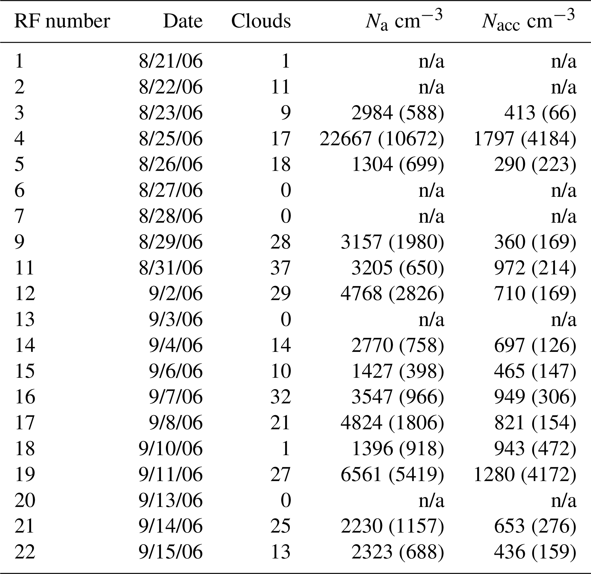
n/a – not applicable.
Table 1 shows each flight conducted during GoMACCS, with the corresponding research flight (RF) number, date, number of clouds in the flight after filtering (including clouds that are only >300 m in length and non-precipitating), the aerosol number concentration (Na, measured by the condensation particle counter, CPC), and the aerosol number concentration for accumulation mode particles (Nacc, measured by the passive cavity aerosol spectrometer probe, PCASP), which includes aerosols that are only in the size range of 0.1 µm < particle size < 2.5 µm. The phase-Doppler interferometer (PDI; see Chuang et al., 2008) was used to collect droplet velocity, size, and measurement time. It was found that the droplet arrival time can accurately be measured to <3.5 µs from Saw (2008), resulting in accurately mapping droplets down to m (assuming average aircraft speed). Note that there is no dead time in PDI measurements. For more information on each of the flights and the instrument payload, see Lu et al. (2008).
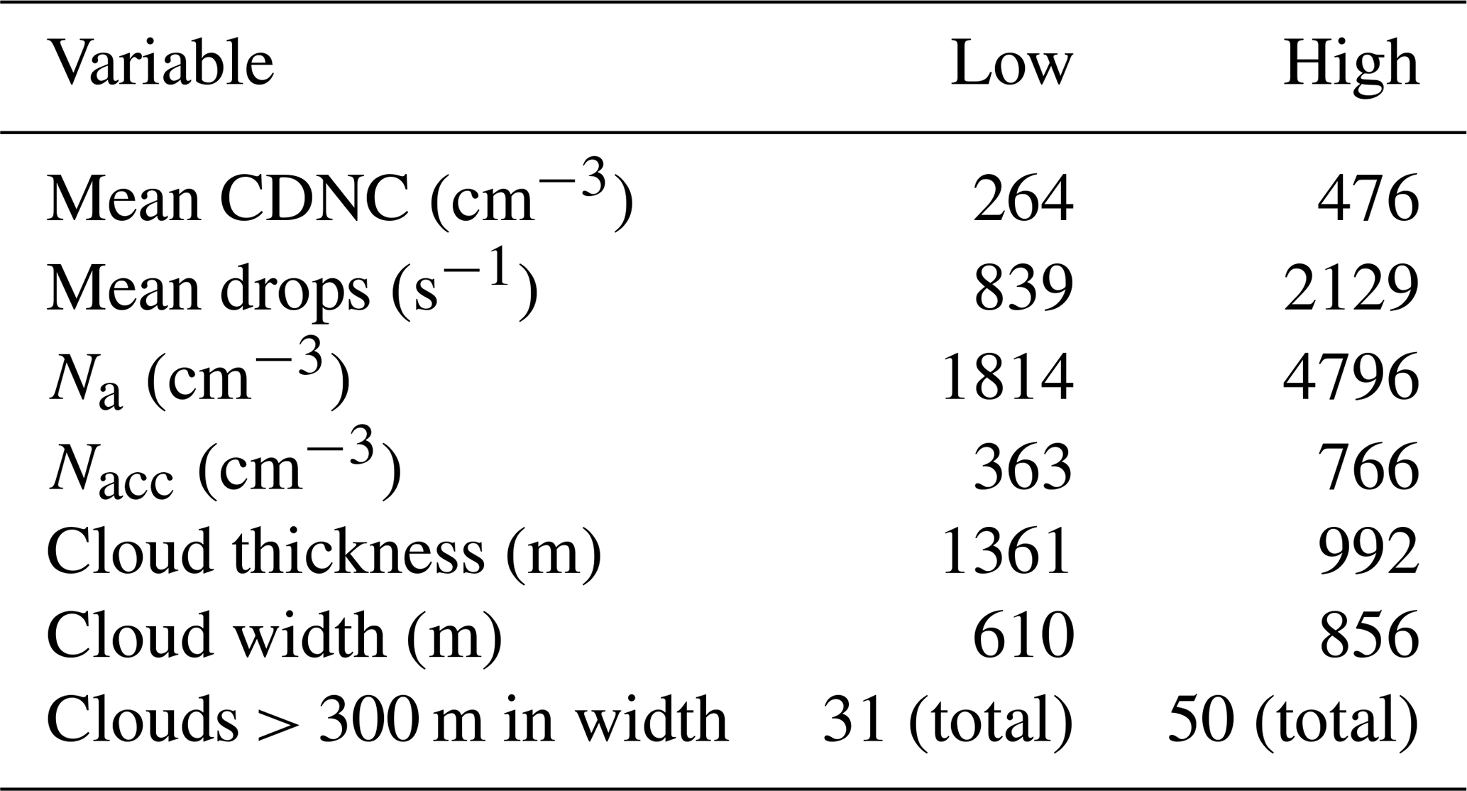
Following the methods in Small et al. (2013), two low (L1 and L2, where L1 (L2) is given by RF 5 (RF 22)) and high (H1 and H2, where H1 (H2) is given by RF 12 (RF 18)) pollution flights were selected out of the 22 research flights. The two least and most polluted flights which had satisfactory cloud sampling were selected for analysis of how aerosol number concentration affects droplet inhomogeneity. A case flight (RF 18) was selected where an isolated cumulus cloud was sampled at different altitudes for analysis of droplet inhomogeneity as a function of cloud height. Table 2 shows variables highlighting different cloud and environmental conditions within each flight. Note that the environmental lapse rate and relative humidity (RH) in Table 2 was calculated from data collected from out-of-cloud spirals, where the average RH was computed for the vertical range of cloud measurements for the respected flight. As a result of RH measurement problems occurring throughout the campaign (i.e., values considerably above 100 %) the RH data were filtered to include values that were only less than 103 %. Table 3 gives a summary of average values for low- and high-pollution cases for select properties from Table 2.
Table 2A summary of cloud, flight, and environmental properties from the L1, L2, H1, H2, and case flights. Note that CDNC stands for cloud droplet number concentration, LWC stands for liquid water content, and mean drops (s−1) represents the mean number of drops measured by the PDI per second. Standard deviation values are represented in parentheses.

n/a – not applicable.
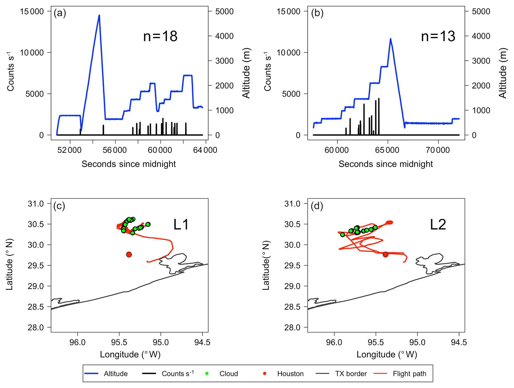
Figure 2L1 and L2 are shown on the left and right, respectively. Flight altitude (blue) as a function of time is displayed in (a) and (b), with droplet counts per second in black. The “n=” represents the number of clouds sampled for each flight after filtering. Panels (c) and (d) show the Texas coast in grey with the location of Houston represented by the red dot. The flight path is outlined in red with the location of clouds displayed by green dots.
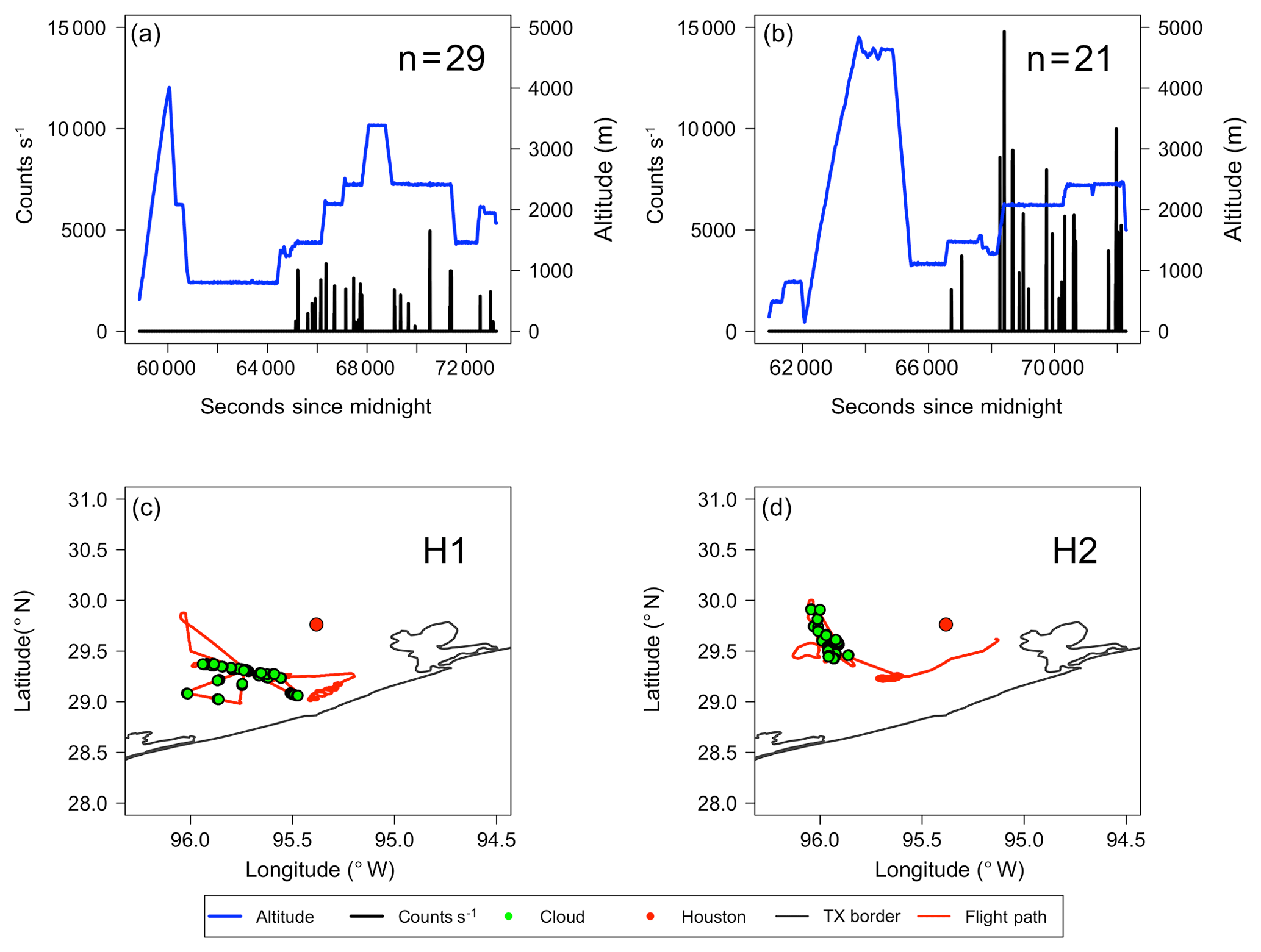
Figures 2 and 3 show the flight altitude as a function of time with droplet counts per second overlaid (panels a and b) and the flight paths (panels c and d) for weakly and highly polluted clouds, respectively. Note that the flight path for the case flight is not shown here. The average droplet counts (clouds) encountered per second (flight) for L1 and L2 were 660 (18) and 1016 (13), respectively, whereas for H1 and H2, the average counts (clouds) encountered per second (flight) were 958 (29) and 3300 (21), respectively. Low-pollution clouds were sampled to the north of Houston (upwind) and high-pollution clouds were sampled to the southwest (H1) and west (H2) of Houston (downwind), as confirmed using archived wind data from the NOAA National Centers for Environmental Information and HYSPLIT trajectories (not shown here) from the Air Resources Laboratory (Stein et al., 2015).
It can be calculated from analyzing Table 3 that the high-pollution clouds had roughly 2.5 times more aerosols per cubic centimeter than the low-pollution clouds. The difference in aerosol number concentration between the low- and high-pollution clouds produces clouds that are statistically different from one another. Figure 4 shows cloud droplet diameter in microns (µm) on the x axis with aerosol number concentration (cm−3) on the y axis, with low-pollution data in green and high-pollution data in gold. Density curves are given to show how the data are distributed for the respected axis. The p value (used to determine statistical significance between two data sets, where p value < 0.05 is considered significant; see Wilks, 2011) between low- and high-pollution cloud droplet size is (average droplet diameter is 13.4 µm (10.7 µm) for low (high) pollution clouds). The linear best-fit trend lines show that droplet size decreases with increasing aerosol number concentration, with R2 values (the proportion of the variance in droplet size that is predictable from the aerosol number concentration) of 0.24 and 0.07 for low and high pollution, respectively. The p value for the aerosol number concentration is . Both properties of the droplet population have p values less than 0.05, making the difference in droplet size and aerosol number concentration significant for the two populations of data. Having two statistically different data populations is ideal for comparing PCF values for low- and high-pollution clouds. If the magnitude of spatial inhomogeneity does not change between the two, then an argument cannot be made for the statistical similarities in the data sets as a possible reason. Note that all p values in this paper were calculated using the Wilcoxon rank-sum test, which is used to determine a statistical difference in the medians of two data sets that have different populations (Wilks, 2011).
Table 3Average values for low (L1, L2) and high (H1, H2) pollution clouds for select variables from Table 2.
4.1 Edge, center, and cloud top inhomogeneities
PCF functions for L1, L2, H1, and H2 are given in Fig. 5, moving from Fig. 5a to d, respectively, with blue (red) representing cloud edge (cloud center) data. The two envelopes represent the 85th and 15th percent quantile of the data. The center lines in each envelope represent the edge and center mean inhomogeneity, with bold mean lines representing data that are statistically significant (p value less than 0.05) and thin mean lines representing data that are statistically similar. The PCF functions for both center and edge data indicate clustering associated with larger-scale inhomogeneity, with the shoulder region of the curves present out to ∼1.2 m before a decrease to zero at spatial scales beyond ∼1.2 m.
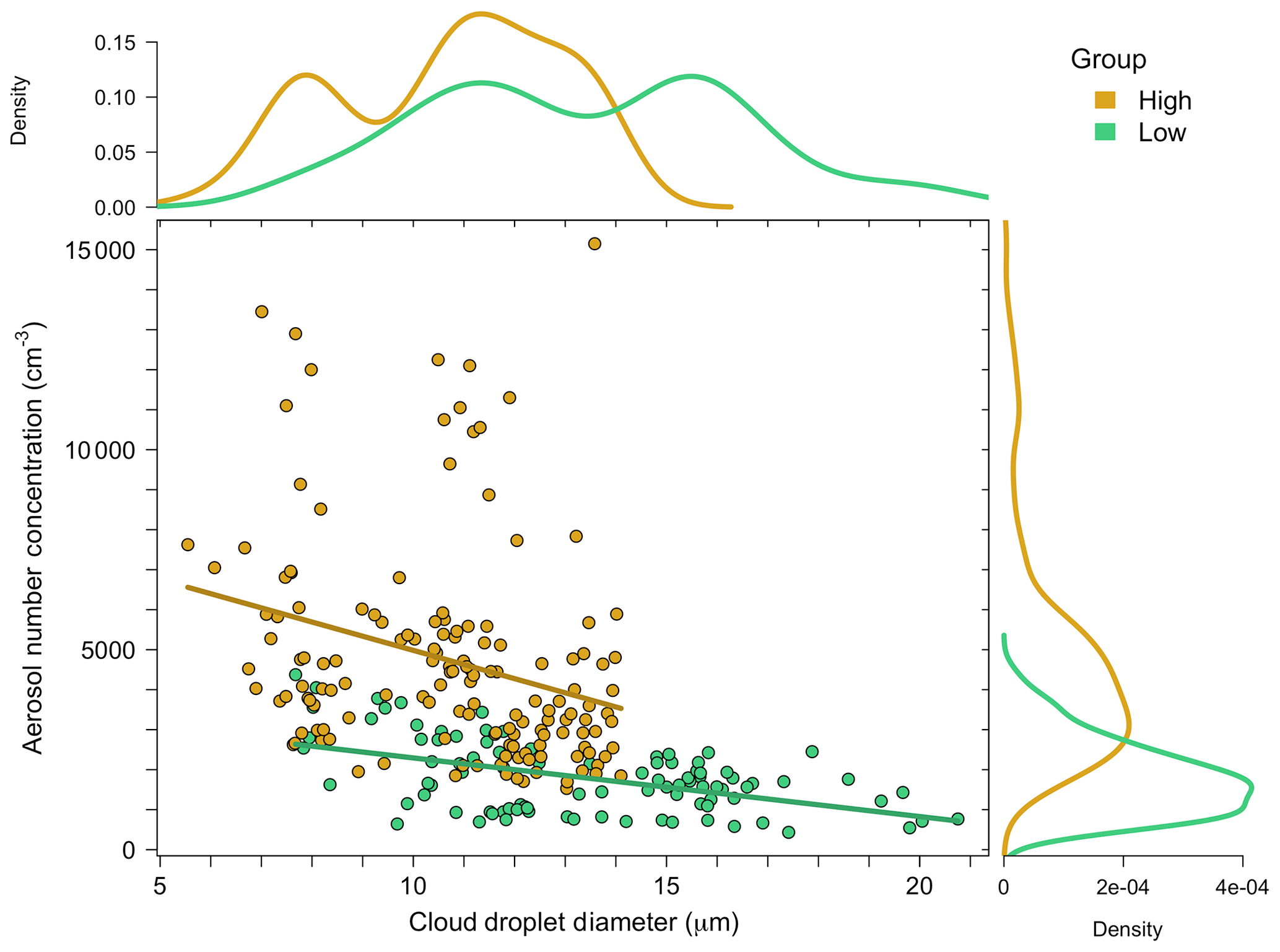
Figure 4Shows cloud droplet diameter (µm) on the x axis and aerosol number concentration (cm−3) on the y axis, with low-pollution data in green and high-pollution data in gold. The corresponding density curves of the high- and low-pollution data are given on the outer margins of the plot.
Table 4The mean PCF, 85th percent quantile, and 15th percent quantile values for center data (on the left) and edge data (on the right) for L1, L2, H1, and H2 in Fig. 5, along with average low and high values from Fig. 9.
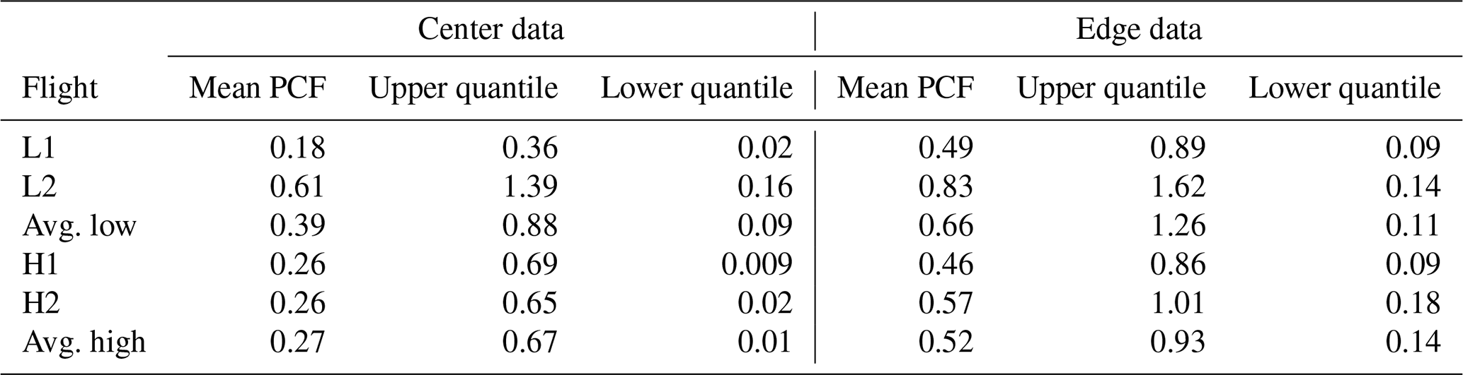
Table 5The mean p value and the percent of data that are statistically significant (for the first 60 PCF values) between edge and center data for L1, L2, H1, and H2 in Fig. 5 and for average low and high in Fig. 9
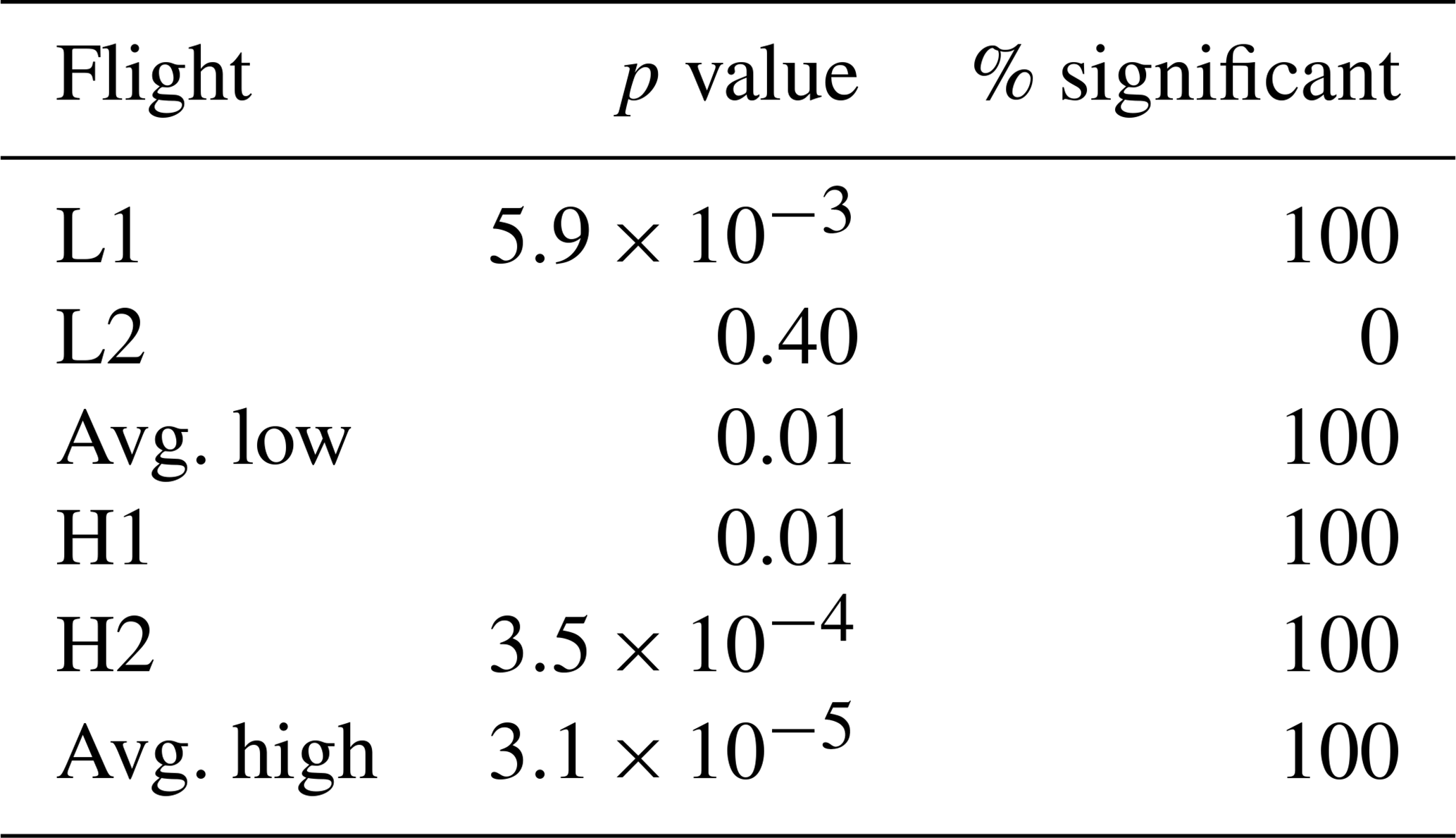
The main takeaway from Fig. 5 is the larger degree of inhomogeneity for cloud edge as compared to the center zones for all four flights. Mean PCF and quantile values for edge and center data can be found in Table 4. The mean and quantile values were calculated by taking the first 60 PCF values (taking PCF values to the left of the green reference line in Fig. 1), covering a spatial scale up to ∼1 m since it is the shoulder region of the PCF curve that we are interested in analyzing. The percent of statistically significant data (for the first 60 PCF values) and the corresponding p values can be found in Table 5. Note that to calculate the p value every PCF curve generated for the respective plot was grouped. A p value was then generated for each spatial lag on the x axis by calculating the Wilcoxon rank-sum test between the two sets of data for the specific x-axis location.
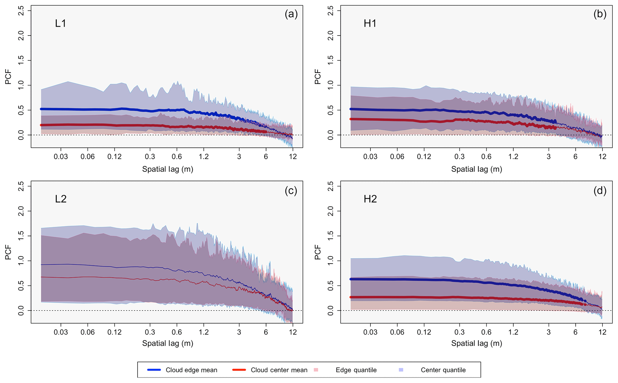
Figure 5PCF clustering signatures for L1 (a), L2 (c), H1 (b), and H2 (d) with spatial lag (m) on the x axis and PCF values (unitless) on the y axis. Edge data are in blue and cloud center data are in red, with the envelopes representing the 85th (a, b) and 15th (c, d) percent quantile values of the data. The mean PCF value for each case is represented by the middle line in each envelope, where a bold mean line represents edge and center differences that are statistically significant.
From analyzing Fig. 5 and the corresponding tables, L1, H1, and H2 show PCF characteristics which are comparable to one another, including the following. (1) The mean PCF value for the edge data is always greater than the mean PCF value for the center data. (2) The 15th percent quantile value for the center data is always smaller than the 15th percent quantile value for the edge data. (3) The 85th percent quantile value for the edge data is always larger than the 85th percent quantile value for the center data. (4) There is a statistical significance between the inhomogeneities occurring between the edge and center zones of the clouds. Note that the statistical significance in the inhomogeneities between the two zones breaks down at larger spatial scales (this is very apparent in the H1 case) as the PCF decays towards zero for both entrainment and center data.
From analyzing L2 (Fig. 5c) and the corresponding tables, there are significant differences from the other three cases. Although the mean edge inhomogeneity is enhanced as compared to the center zone, the difference is not statistically significant, with 0 % of the data having a p value below 0.05 (average p value of 0.40). Another difference is the range of the quantile values, with the cloud edge data having a lower 15th percent quantile value than that of the center data, in contrast to what is observed in L1, H1, and H2. Note that the mean inhomogeneity amount for L2 (both center and edge) is enhanced as compared to the other three cases (Table 4).
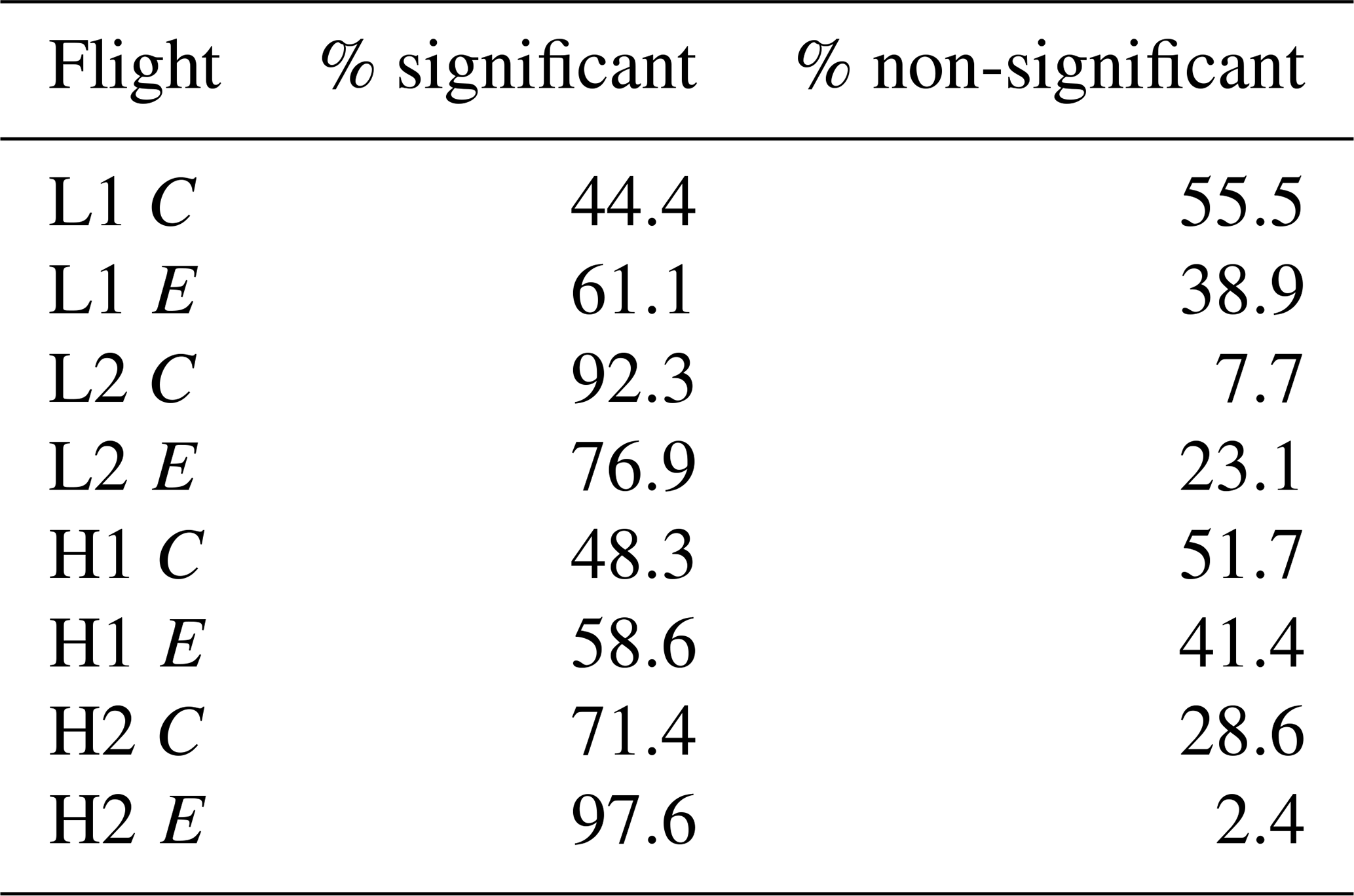
It is clear that there are enhanced inhomogeneities in the edge zone as compared to the center zone, but one needs to understand how to define if the overall inhomogeneities (both edge and center) are significant as compared to a randomly distributed droplet population. This is done by analyzing the range that the PCF can take on due to the random nature of the data. If the physical inhomogeneities measured fall outside of this range, then the conclusion can be made that the droplet spatial inhomogeneities being viewed are indeed real and not perfectly homogeneous. This test was performed on each of the four cases, following the methods outlined in Larsen and Kostinski (2005). For the data, 1000 Poisson simulations were produced (as is seen in Fig. 1b, showing a single Poisson simulation) using the same time duration and droplet count as the original data. These Poisson simulations then form an envelope of PCF values (using the maximum and minimum values from the 1000 simulations) one would consider homogeneous. PCF values that lie within the Poissonian simulation envelope were recorded by using the average PCF value and were labeled non-significant. Table 6 shows the percentage of PCF values for each flight and each location (edge and center) that were considered non-significant and significant. From analyzing Table 6 it can be seen that not every cloud section measured experienced inhomogeneity that would be considered a statistical difference from a random distribution. However, a majority of the data sets do display inhomogeneities that are statistically significant, with the exception of the L1 center and H1 center data, which shows that less than 50 % of the droplet populations display statistically significant inhomogeneities. With the exception of the L2 case (which does not have a statistical difference between edge and center inhomogeneity), the center inhomogeneity contains a higher percentage of PCF values that are non-significant as compared to the edge data.
Table 6Percentage of inhomogeneities that are significant and non-significant (as compared to a randomly distributed droplet population) for center (C) and edge (E) data in L1, L2, H1, and H2.
We can use the inter-arrival times used in calculating the PCF to develop a better understanding of the overall droplet spatial distributions and the largest inhomogeneities measured by directly analyzing the inter-arrival time distribution (as is done in Baker, 1992). Figure 6 shows the inter-arrival distance (IAD, distance between each droplet measurement) binned for L1 and zoomed in on a frequency of 60 as to put more emphasis on the largest IADs measured. Zooming in further on the first bin (range of 0 to 60 cm), where 98.4 % and 99.5 % of the data lie for edge and center data, respectively, it can be seen that the IADs follow a Poisson distribution. Analyzing the largest IADs, the box plot in the top left corner shows the data for center and edge that is greater than or equal to the 0.998 quantile of the IAD data, i.e., the largest 0.2 % of the IAD data. This results in approximately the largest 100 IADs to be represented in the box plot.
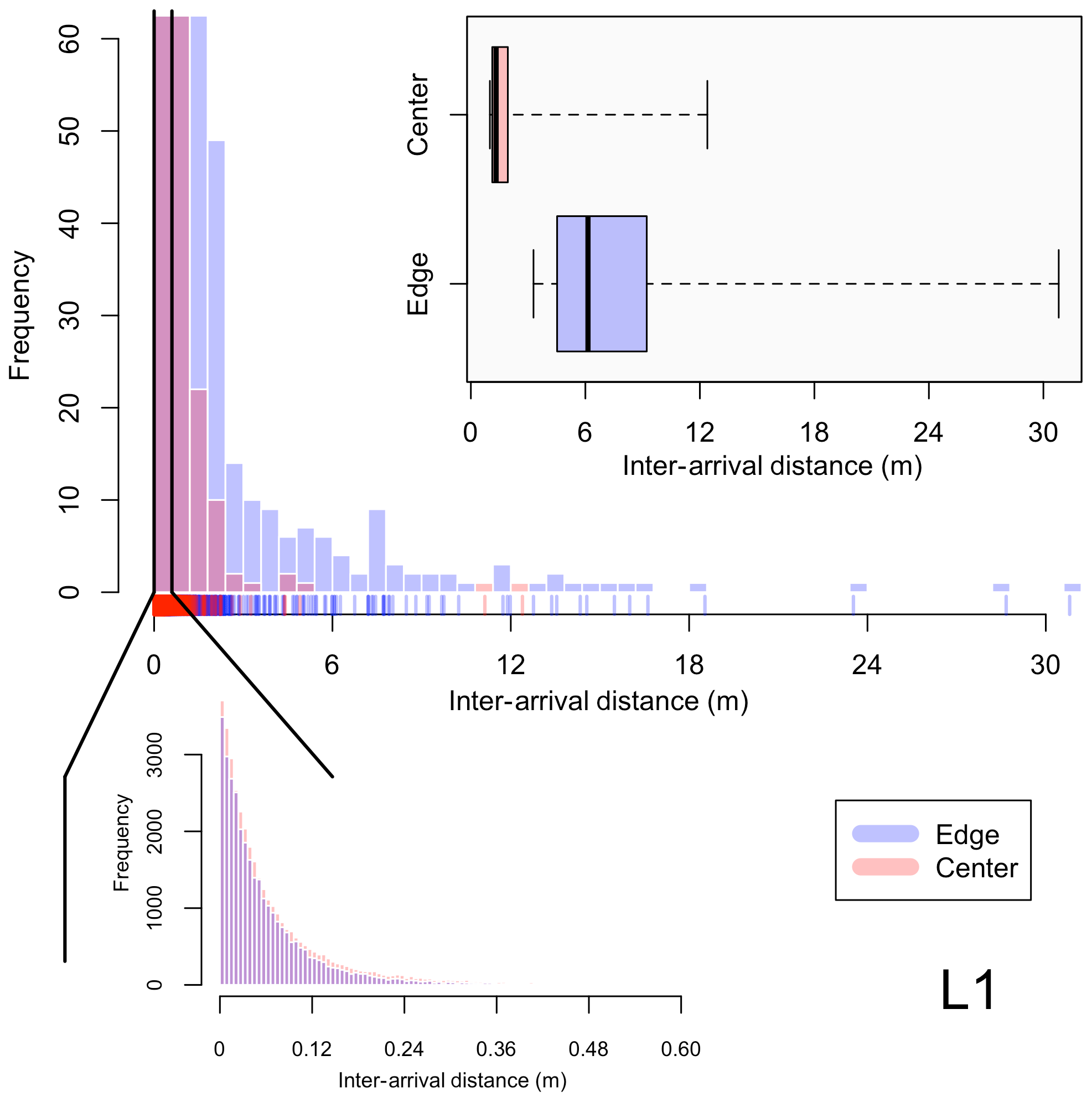
Figure 6Histogram distributions of the inter-arrival distance (IAD) for droplet populations measured in flight L1, with edge data in blue and center data in red. Note that the main histogram is zoomed in to a value of 60 on the y axis, with further analysis of the first bin (representing a range from 0 to 0.60 m) below the main histogram. The box plots in the top right represents the IAD data that are greater than or equal to the 0.998 quantile of the overall data sets for entrainment and center.
Although the raw histograms of IAD data are not displayed for L2, H1, and H2 (they appear very similar in nature to that of L1), the resulting box plots of the IAD data which are greater than or equal to the 0.998 quantile for each of the four flights are presented in Fig. 7, where the tick marks occurring on the upper whiskers represent the raw data positions for a better visualization of how the data are distributed. For each of the four flights, the edge data are shifted to larger IAD values as compared to the center data, with the IADs between the edge and center data being statistically significant for each of the four cases. Note that the median value for each data set is displayed within the box plot. This tells us that there are more numerous, larger pockets of droplet-free air within the edge zone as compared to the center zone. For example, in analyzing the box plots for L2, we can see that there are five cases where there is a distance of 20 m or greater between droplet measurements for the edge zone, as compared to only one case for the cloud center zone.
Table 7Values for vertical velocity (m s−1), RH (%), LWC (g m−3), the PCF, and the median drop size (µm), respectively, for each normalized cloud height in Fig. 8.
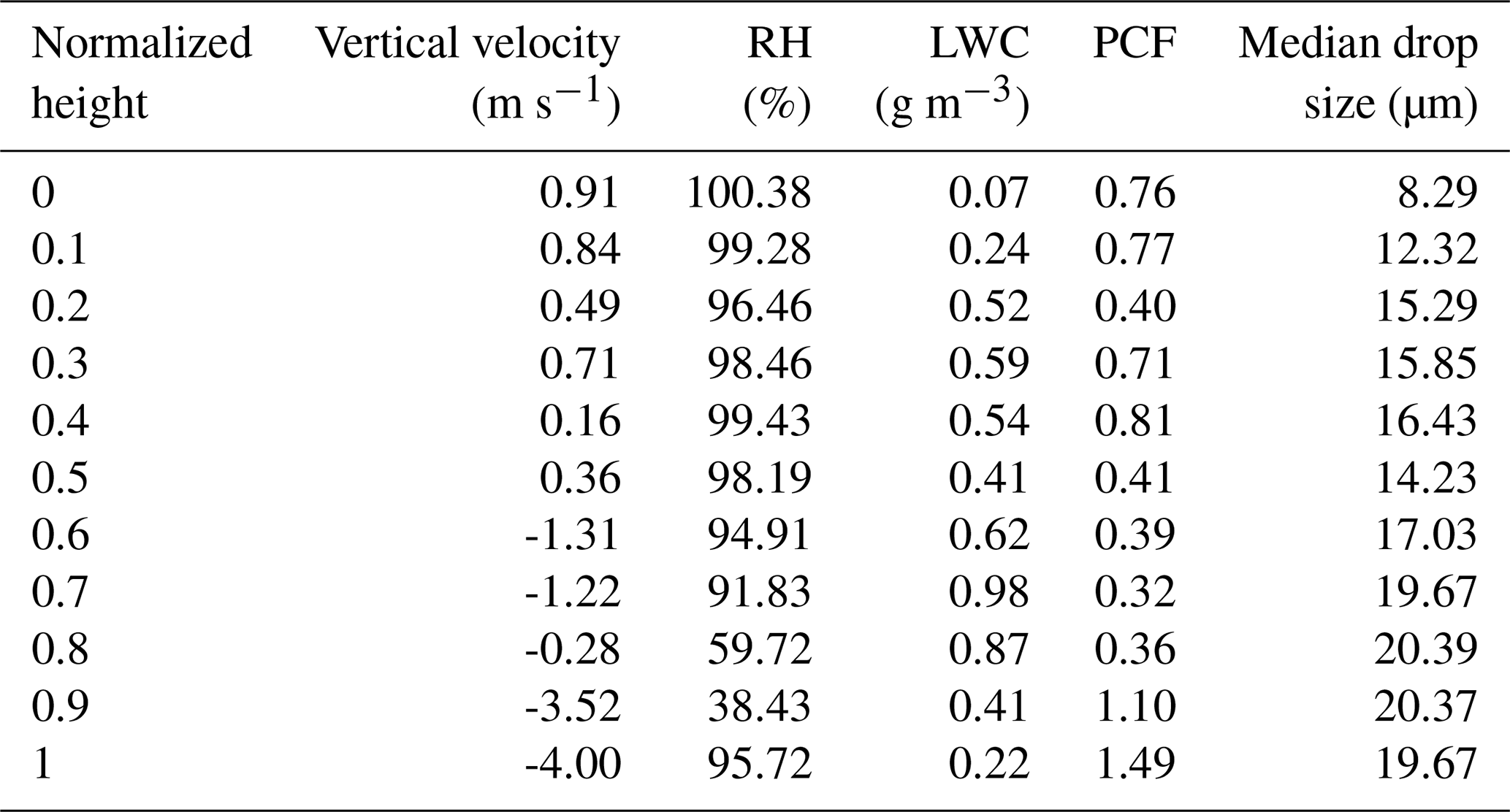
Figure 8 shows how the mean PCF value (where, again, the mean PCF value is obtained by taking the mean of all individual PCF values to the left of the green reference line in Fig. 1) and other environmental properties (cloud droplet number concentration, cm−3; liquid water content, g m−3; RH, %; and vertical velocity, m s−1) vary with normalized cloud height from the case flight. Variable quantities for each normalized cloud height can be found in Table 7. The liquid water content (LWC) increases from cloud base (0.073 g m−3) to a normalized cloud height of 0.7 (0.98 g m−3) before decreasing to 0.23 g m−3 at cloud top. Accompanied by the decrease in LWC is a sharp decrease in the RH from 91.8 % to 38.4 % between normalized cloud heights of 0.7 and 0.9, before increasing again at cloud top to 95.7 %. As both the LWC and RH decrease, the PCF has a sharp increase from 0.36 to 1.49 between normalized cloud heights of 0.8 and 1.0, indicating enhanced inhomogeneity at cloud top. The PCF values at cloud top (between normalized cloud heights of 0.8 to 1.0) are statistically significant as compared to the PCF values below a normalized altitude of 0.8 (with a p value of 0.043), making the inhomogeneity that is present at cloud top statistically significant from the inhomogeneity that is occurring in lower cloud layers.
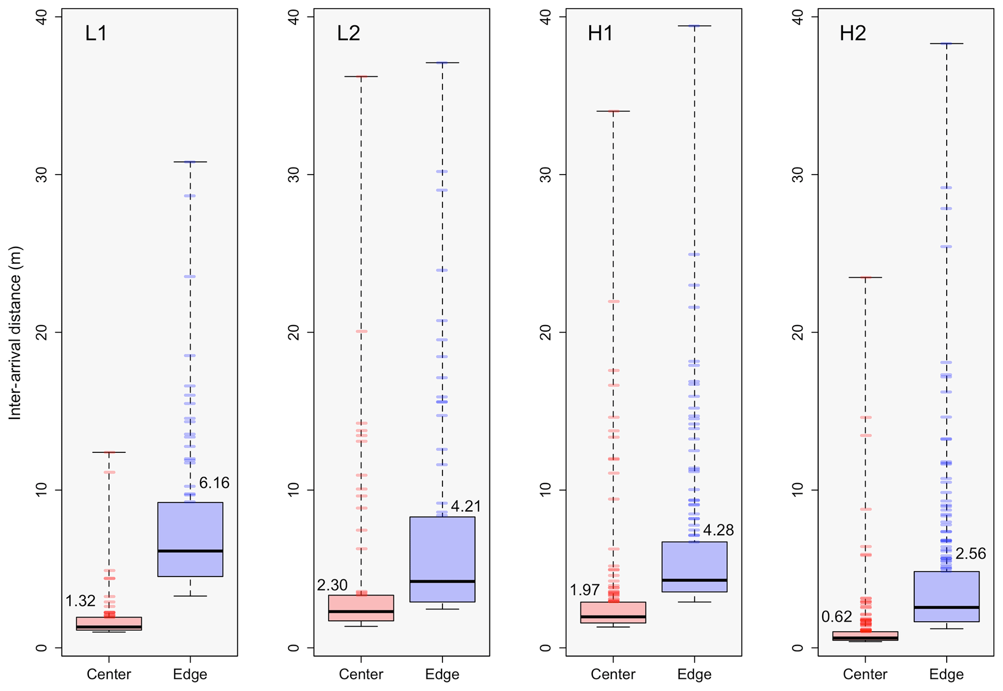
Figure 7Box plots for the IAD data which are greater than or equal to the 0.998 quantile of the overall data sets for edge (blue) and center (red), with L1, L2, H1, and H2 shown moving from left to right, respectively. The median value for each data set is displayed within the plot. Tick marks occurring on the upper whiskers represent the raw data positions. Note that panel L1 represents the same box plot displayed in Fig. 6.
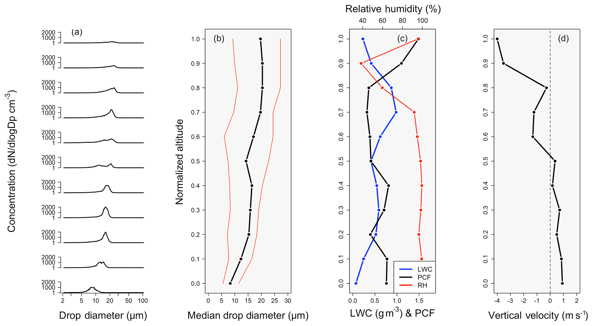
Figure 8Shows the cloud droplet size distribution in panel (a). Panel (b) gives the median droplet size along with the 5th and 95th percent quantiles (red) of the droplet size distribution. Panel (c) shows LWC (blue), RH (red), and the mean PCF value (black). Panel (c) shows vertical velocity. All variables are represented as a function of cloud normalized altitude.
Figure 8a gives the cloud drop size distribution for each normalized cloud height while Fig. 8b gives the median droplet diameter along with the 5th and 95th percent quantiles of the drop size distribution. The median drop size increases from 8.29 µm at cloud base to 19.67 µm at cloud top. In comparing the median drop size to the mean PCF value for each normalized height, the R2 value is 0.041, indicating no correlation between the PCF and median droplet size. Particulary at cloud top where the PCF increases, there is no associated changes in the median drop size or the quantile values of the size distribution. Figure 8d shows that the vertical velocity is negative in the upper portion of the cloud, while an updraft is present in the lower 50 % of the cloud.
4.2 Low- vs. high-pollution inhomogeneity
Figure 9 panels (1a) and (1b) give the same information as in Fig. 5, except for the PCF values for total low pollution (average of L1 and L2) and total high pollution (average of H1 and H2), respectively. The characteristics of the two clustering signatures are similar to that of Fig. 5. The average PCF values for low- and high-pollution edge and center data can be found in Table 4, along with the 15th and 85th percent quantile values. Table 4 reveals that the mean PCF values (for both edge and center data) for the low-pollution case are larger than the corresponding mean PCF values for the high-pollution case. As can be seen in Table 5, 100 % of the first 60 spatial lags are statistically significant for both average low- and high-pollution cases between the edge and center data.
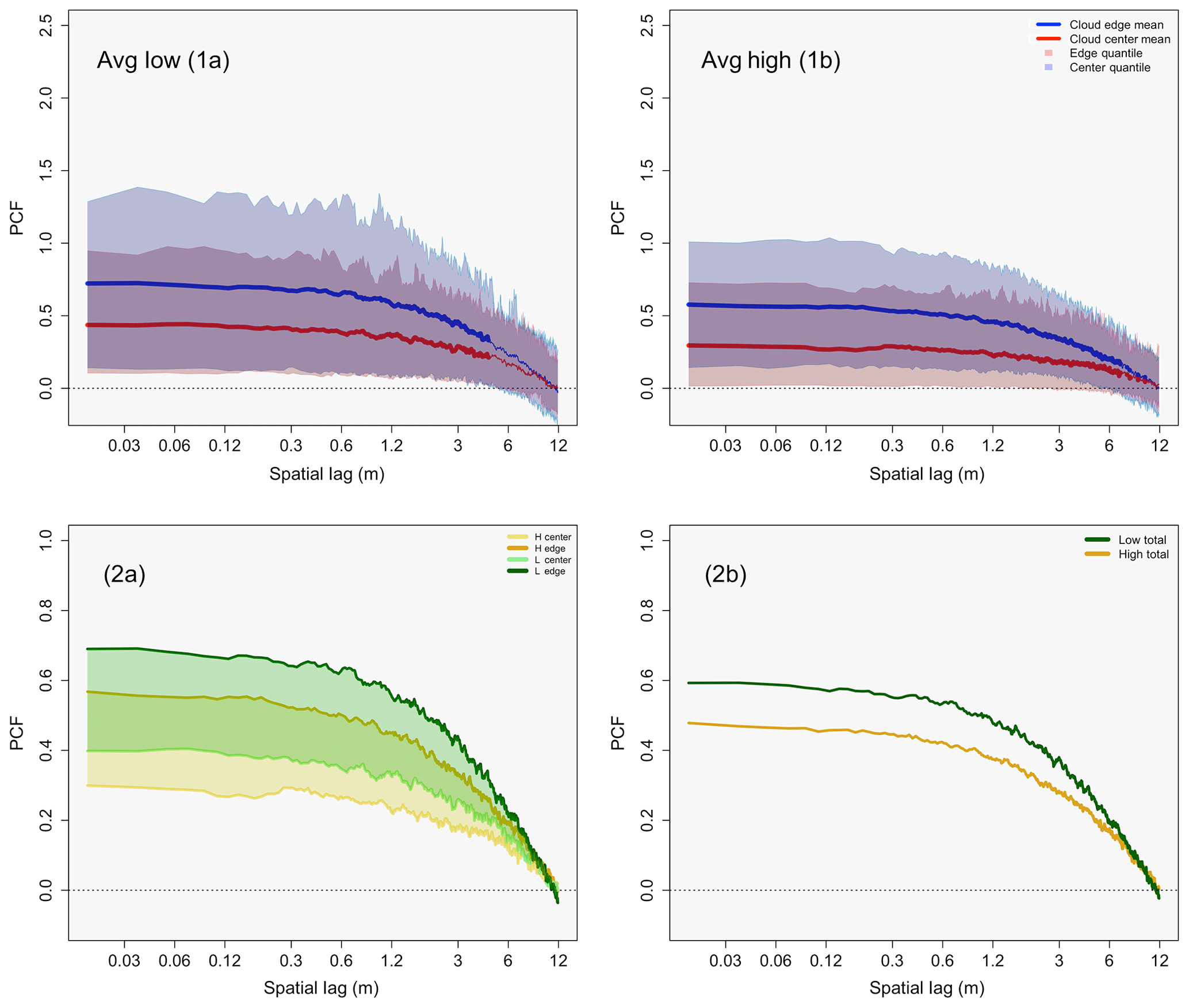
Figure 9Panels (1a) and (1b): as in Fig. 5, except for average low-pollution PCF values (L1, L2) in panel (1a) and average high-pollution PCF values (H1, H2) in panel (1b). Panels (2a) and (2b): low-pollution data in green and high-pollution data in gold. Panel (2a) shows envelopes that span the mean center PCF value (lower limit of the envelopes) to the mean edge PCF value (upper limit of the envelopes). Panel (2b) gives the overall mean PCF for low- and high-pollution clouds.
The larger mean inhomogeneity amount for the low-pollution clouds can be seen well in Fig. 9 panel (2a), which shows low-pollution data in green and high-pollution data in gold. The boundaries of each green and gold envelope are created by the mean center (bottom of each envelope) and edge (top of each envelope) inhomogeneity. Low-pollution clouds are clearly offset to a higher inhomogeneity amount for both mean center and edge inhomogeneity. Figure 9 panel (2b) shows the overall mean of all the PCF values for low- and high-pollution clouds. The overall mean PCF value for low-pollution clouds (average of entrainment and center inhomogeneity for both L1 and L2) is 0.54, while the overall mean PCF value for high-pollution clouds is 0.43. Although it appears that low-pollution clouds experience more inhomogeneity as compared to high-pollution clouds, the difference is statistically similar. The average p value is 0.19 for the first 60 spatial lags, with 0 % of the data being statistically significant.
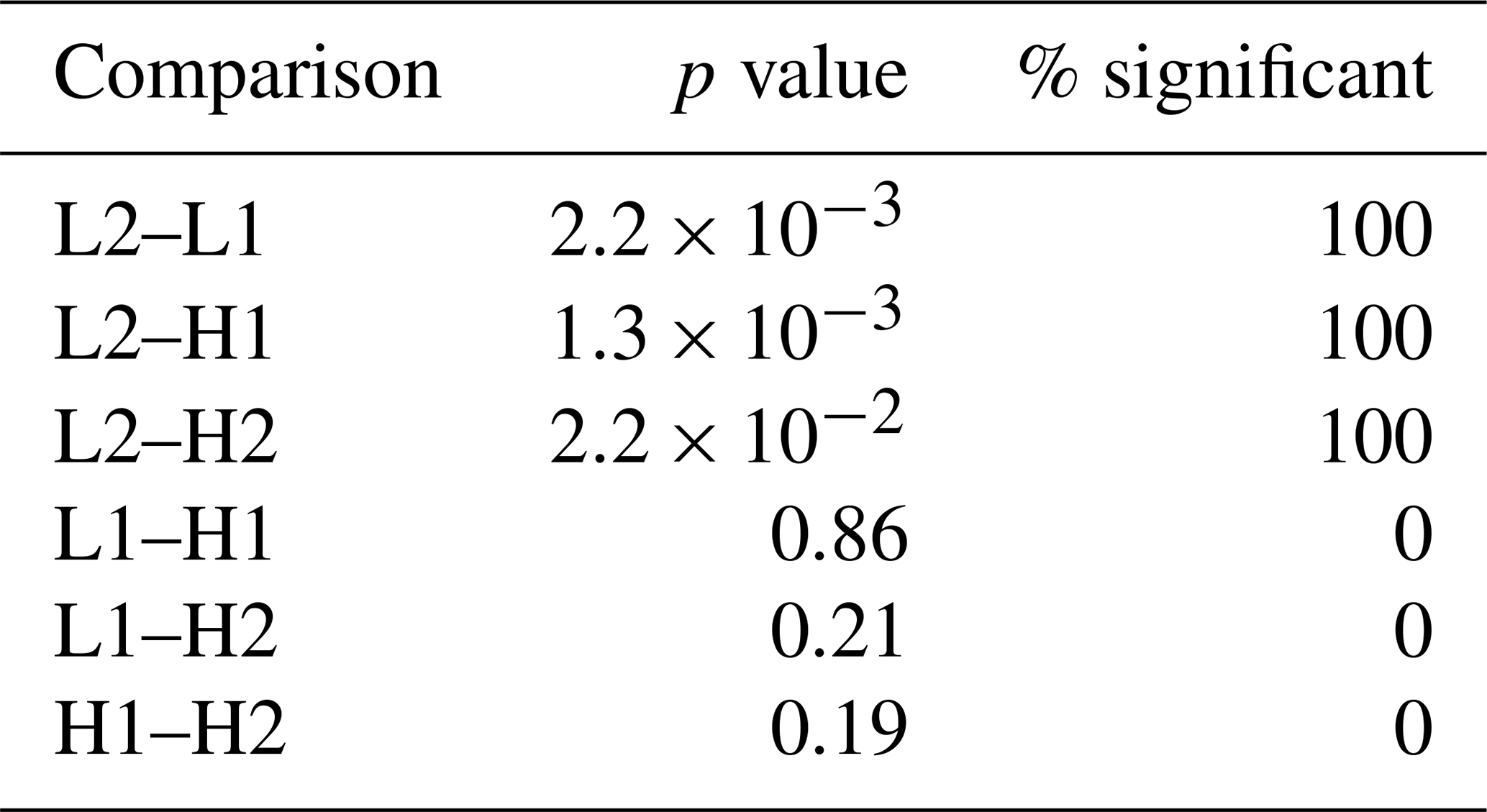
Low-pollution clouds have a non-statistically significant higher amount of inhomogeneity than high-pollution clouds, with further analysis showing that the higher amount of inhomogeneity in the low-pollution case is due entirely to the L2 flight. Figure 10 gives the same information as panels (2a) and (2b) in Fig. 9, except for the individual flights (L1, L2, H1, H2) shown. From analyzing Fig. 10a, one can see the mean center and edge inhomogeneity for L2 (light green envelope) is beyond the range of the other three flights. The total mean PCF for the clouds in L1, L2, H1, and H2 is shown in Fig. 10b. L2 has a mean PCF value of 0.76, which is roughly twice the mean PCF values (and statistically significant; see Table 8) of the other three flights, where L1 (dark green), H1 (dark gold), and H2 (light gold) have mean PCF values of 0.39, 0.40, and 0.46, respectively. The question of whether inhomogeneity depends on aerosol number concentration cannot confidently be answered. Although Fig. 9 shows that low-pollution clouds have a larger amount of inhomogeneity, statistically speaking the inhomogeneity between low- and high-pollution clouds is the same. Further analysis shows that L1, H1, and H2 all have statistically similar inhomogeneity values (see Table 8) with mean inhomogeneity amounts that are almost identical. Flight L2 has statistically significant inhomogeneity as compared to the other three cases and is solely responsible for causing the low-pollution clouds to have a higher mean PCF value than that of the high-pollution clouds.
Table 8The mean p value and the percent of data that are statistically significant (for the first 60 PCF values) between PCF functions provided in Fig. 10b.
5.1 Cloud lifetime hypothesis and inhomogeneity in L2
An explanation for the statistically different inhomogeneity in L2 as compared to the other three cases could be cloud age. A study by Schmeissner et al. (2015) found that dissipating clouds have five main characteristics, including a negative buoyancy (m s−2) and vertical velocity, lower LWC and cloud droplet number concentrations (CDNC) as compared to actively growing clouds, and a larger RH shell around the cumulus cloud. Decaying clouds are also associated with the enhanced entrainment of dry air, where Cooper and Lawson (1984) found that the LWC decreases due to entrainment as cumulus clouds deteriorate. Lu et al. (2013) and Cheng et al. (2015) also found that enhanced entrainment leads to decreases in cloud droplet concentration, droplet size, and LWC.
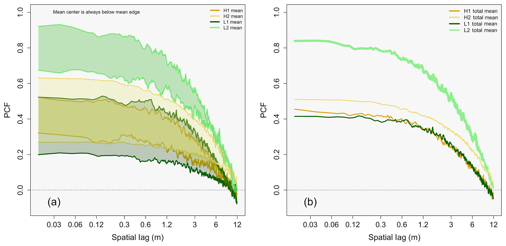
Figure 10As in panels (2a) and (2b) from Fig. 9, except for the individual flights of L1 (dark green), L2 (light green), H1 (dark gold), and H2 (light gold). Note that the envelopes in panel (a) represents the range from the mean center inhomogeneity (lower limit of each envelope) to the mean edge inhomogeneity (upper limit of each envelope).
Figure 11 shows box plots of vertical velocity, LWC, cloud width, CDNC, buoyancy, and RH. Red median lines represent data sets that are statistically different when compared to L2. Note that, except for cloud width, each variable is represented from 1 Hz data collected during in-cloud sampling. From analyzing Fig. 11 (exact median values for variables can be found in Table 9), L2 has the lowest median vertical velocity, LWC, cloud width, and CDNC, with L2 being statistically significant (p values found in Table 10) when compared to the other three flights. The fact that L2 has the lowest median vertical velocity reflects the fact that clouds have smaller positive vertical velocities than those measured in the other three flights, suggesting weaker growth potential. The low LWC in L2 signifies that entrainment of dry air has been occurring, resulting in the evaporation of liquid water droplets, reducing the LWC and the CDNC (Pruppacher and Klett, 1997). Although Schmeissner et al. (2015) does not discuss cloud width, clouds that are dissipating would be expected to have a smaller horizontal extent due to entrainment of dry air leading to evaporation of cloud edge droplets as compared to mature clouds.
Table 9Median values of vertical velocity (m s−1), LWC (g m−3), cloud width (m), CDNC (cm−3), buoyancy (m s−2), in-cloud RH, and out-of-cloud RH (%) from Fig. 11.
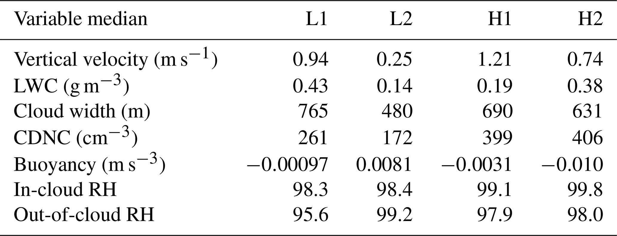

Figure 11Box plots of L1, L2, H1, and H2, represented in that order on the x axis, with panels (a) through (f) representing vertical velocity (m s−1), LWC (g m−3), cloud width (m), CDNC (cm−3), buoyancy (m s−3), and in-cloud RH (%), respectively. Red median lines represent data sets that are statistically significant as compared to the L2 data set. Each red dot in panel (f) represents out-of-cloud RH.
Figure 11f gives a box plot of in-cloud RH, with L2 having the second-lowest in-cloud RH, while being statistically similar to that of the other three flights. The red dots represent the median out-of-cloud RH (100 m before and after cloud edge). L2 is the only flight where the RH increases out of the cloud. The fact that the RH is larger, on average, outside of the clouds in L2 as compared to inside of the clouds could be a sign of a large humid shell that is surrounding the individual clouds. The humid shell results from entrainment of dry air into the cloud while moist air is detrained out of the cloud into the cloud-free environment, resulting in a lower (larger) RH inside (outside) the cloud (Heus and Jonker, 2008; Jonker et al., 2008; Heus et al., 2008). More evidence for the large humid shell can be gathered from the vertical profiles of environmental RH reported in Table 2, where the average RH (measured out of cloud) for the vertical range of cloud measurements was 96.3 % for L2, while for the other flights the RH was considerably lower.
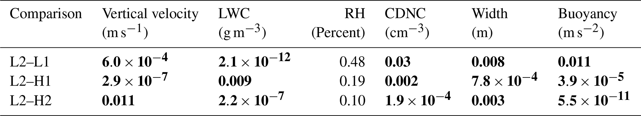
Figure 11e shows the in-cloud buoyancy, which was calculated by taking the in-cloud and out-of-cloud (100 m before and after cloud edge) virtual potential temperatures. L2 has the largest median buoyancy and is statistically significant as compared to the other three flights. The clouds in the L2 flight have five out of the six characteristics for decaying clouds, including the (1) lowest vertical velocity, (2) lowest LWC, (3) lowest CDNC, (4) lowest cloud width, and (5) largest humid shell. The evidence points to the clouds in L2 decaying on average, therefore leading to larger droplet inhomogeneities as more dry air is mixed into the clouds as compared to the other three cases. The statistically similar values between center and edge inhomogeneities for L2 add to the cloud lifetime hypothesis, as it is not only the cloud edge zone that is experiencing mixing but the entire horizontal extent of the clouds (both edge and center zones) that is experiencing mixing and dissipation. However, one would expect the buoyancy of dissipating clouds to be negatively buoyant, not positively buoyant as is shown. Although cloud age is a good hypothesis in describing the higher inhomogeneity amounts measured in the L2 flight, the data presented do not offer a conclusive resolution.
Table 10The p values between L2 and L1, L2 and H1, and L2 and H2 for in-cloud vertical velocity (m s−1), LWC (g m−3), RH (%), CDNC (cm−3), cloud width (m), and in-cloud buoyancy (m s−2). Statistically significant values are presented in bold.
Aerosols can act as cloud condensation nuclei (CCN), increasing the number of droplets in clouds and decreasing the mean droplet size (Twomey, 1977). Although not shown in Fig. 11, for the clouds measured in this study the median droplet size was 15.01 (L1), 11.45 (L2), 11.19 (H1), and 10.92 µm (H2). Although L2 has roughly half the aerosol number concentration as that of H1 and H2, the droplet size for L2 is more comparable to that of the high-pollution flights as compared to L1. This suggests that some physical process is resulting in the droplet sizes of L2 being smaller than what is expected based on the reported Na values. The most likely explanation is the entrainment of dry air leading to enhanced evaporation.
Other possible explanations for the increased inhomogeneity in L2 could be due to flight path or the atmospheric environment for a given flight. The flight path through the cumuli for L2 could have favored cloud edge or cloud top instead of true cloud center. Favoring cloud edge would result in measuring areas of cloud that favor a higher amount of inhomogeneity (as displayed in Fig. 5) and could result in the overall larger average amount of inhomogeneity experienced. Measuring just cloud edge would result in a lower vertical velocity, LWC, and CDNC due to evaporation from entrainment and a shorter cloud width from not traversing the maximum diameter of the cloud. However, just as with the cloud lifetime hypothesis, the buoyancy is expected to be negative, not positive, in the edge zone of the cloud due to evaporational cooling of the air.
Comparing cloud width on different days can become complicated due to the environmental factors that control cloud size. As is discussed in Hill (1973) and Seigel (2014), the dominant factor governing the size and spatial distribution of cumulus clouds is the size and strength of the sub-cloud circulations. There is no way to know what the sub-cloud circulation was for the given days. Only vertical velocity is available, which, as we saw in Fig. 11a, was smallest for the in-cloud portions of the L2 flight. Whether the fact that L2 clouds were smaller as compared to the other flights is due to dissipation through entrainment of dry air or environmental characteristics is unknown.
5.2 Edge vs. center inhomogeneity and aerosol number concentration
The finding that droplet spacing is inhomogeneous agrees with the findings in multiple other papers, including Good et al. (2012), Ireland and Collins (2012), and Saw et al. (2012). Note that in this paper inhomogeneity is measured down to ∼2 cm. It is expected from the inertial clustering hypothesis that droplet clustering continues to increase at scales below what was measured here – into the millimeter scales (Shaw, 2003) due to inertial clustering from fluid vorticity. It is important to note, however, that not all the inhomogeneities measured were statistically different from a random Poisson distribution. Only 60.8 % of the traverses for center data showed a statistical deviation from a randomly distributed droplet population, as compared to 72.2 % for edge data. This suggests that although a majority of the data display large-scale inhomogeneity, 31.7 % of the data are randomly distributed. This is partially in agreement with Chaumat and Brenguier (2001), which found that droplets displayed homogeneous distributions on small and large scales.
PCF curves measuring inertial clustering in other literature (Larsen, 2007; Shaw, 2003; Shaw et al., 2002) show an elevated value of the PCF at the smallest separations that is naturally accompanied with lower values of the PCF at larger separations. The PCF curves presented here are measured over separations ranging from 2 cm (just above the Kolmogorov scale) to 12 m (on the order of the integral scale) and show elevated values over a large spatial range (2 cm to 1.2 m) before the PCF begins to decay. It is important to keep in mind that this suggests that the elevated PCF values examined here are the result of spatial holes in the droplet concentrations (non-stationary) due to mixing with dryer air and not preferential concentration from particle inertia. Note that other possible causes of larger-scale inhomogeneity that are not examined here include fluctuations in the vertical velocity and cloud condensation nuclei (Pinsky and Khain, 2002, 2003).
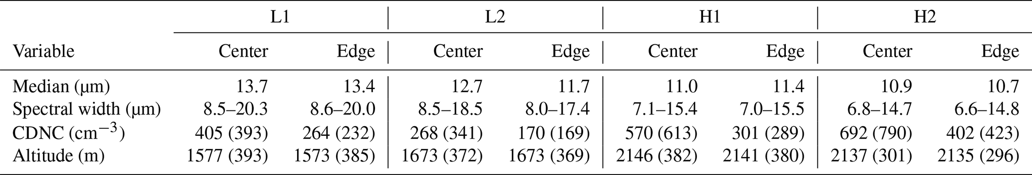
From the clouds measured, the conclusion can be made that droplet inhomogeneity does change as a function of cloud center vs. cloud edge, with the edge zone having a larger amount of inhomogeneity than the center of the cloud, which is shown to be statistically significant. The decrease in inhomogeneity in the center of the cloud as compared to the edge may be attributed to several aspects, including (1) the mean entrainment rate decreases from cloud edge to cloud center, as has been shown with in situ measurements made by Cheng et al. (2015). Although the entrainment rate is not directly measured here, an analysis of the type of entrainment that is occurring is provided in Table 11. It can clearly be seen from Table 11 that the median droplet size along with the spectral width of the drop size distribution is virtually the same between the center and edge zones for each respective flight. This suggests that the drop size distribution is unshifted between center and edge zones. The CDNC is reduced for the edge zone as compared to the center zone for each of the four cases, however, with percent reductions of the CDNC in the edge zone of 35 %, 40 %, 47 %, and 42 %, for L1, L2, H1, and H2, respectively. The unshifted drop size distribution along with a reduction in the CDNC at cloud edge is evidence of the occurrence of inhomogeneous mixing. The fact that the CDNC is reduced at cloud edge suggests increased evaporation at the edge zone due to enhanced mixing with dry air as compared to cloud center. The altitude between edge and center zones for each respective flight is virtually the same, suggesting that the analysis conducted on the drop size distribution is not affected by differences in altitude. (2) Turbulent mixing within the cloud leads to a breakup of the larger-scale inhomogeneities, reducing the PCF. Ireland and Collins (2012) through simulations observed a larger degree of non-uniformity for a turbulent–non-turbulent interface (i.e., cloud edge) as compared to a turbulent–turbulent interface (i.e., cloud center) due to the lower turbulence levels at the edge weakening the homogenization process of the droplet spacings.
Table 11Provides the median value and spectral width (10th to 90th percent quantile range) of the drop size distribution, the altitude at which measurements occurred, and the cloud droplet number concentration (CDNC) for both the center and edge zone of cloud passages for each of L1, L2, H1, and H2. Standard deviation values are given in parenthesis.
Along with enhanced inhomogeneity at cloud edge, enhanced inhomogeneity at cloud top is also evident due to entrainment as is shown in Fig. 8, where the LWC and RH have a sharp decrease near cloud top accompanied by an increase in the PCF. The decrease in RH and LWC is characteristic of dry air being entrained into the cloud. The entrainment at cloud top can also be seen to cause a negative vertical velocity (from evaporative cooling, typically termed cloud top entrainment instability) in the upper portion of the cloud (Fig. 8c), where the average vertical velocity is increasingly negative above a normalized cloud height of 0.5, suggesting penetrative downdrafts extend into the middle section of the cloud.
Although the conclusion in this paper is that aerosol number concentration does not affect droplet inhomogeneity, this conclusion can only be made for the range of Na given and the resulting mean droplet sizes. For example, Xue and Feingold (2006) showed that smaller droplets evaporate more readily, leading to dissipation of the cloud through entrainment. However, in Xue and Feingold (2006) the difference in droplet size was roughly −81 % between clean and polluted clouds. Although the difference in droplet size is statistically significant between flights, the largest percent difference analyzed here is only −28 % between flights L1 and H2. Perhaps the aerosol number concentration can affect the amount of clustering that is occurring if there are more significant changes in the sizes of the droplet populations than those analyzed here. Such a case could be comparing a highly polluted cloud in Houston (mean droplet diameter ∼11 µm) to a clean cloud over the ocean (mean droplet diameter ∼35 µm, as was found for some Atlantic trade wind cumuli; Wang et al., 2009). This would result in droplet populations that have a large enough percent difference in their size that evaporative effects may be severe enough to lead to statistically different entrainment rates and droplet inhomogeneity. However, sampling clouds in two different types of boundary layers would result in vast differences in their environmental characteristics. One way in which sampling could be achieved would be to analyze cumuli that are exposed to a point source of pollution (such as volcanic gas emissions in Hawaii) in the marine boundary layer and cumuli that lie outside the pollution plume. This would allow for the sampling of clouds which are exposed to vast differences in Na but still share many of the same environmental characteristics.
Flight data obtained from the CIRPAS Twin otter aircraft flown during the GoMACCS campaign near Houston, TX, from 2006 were used to investigate 81 non-precipitating cumulus clouds, and one vertically developed cumulus cloud, to better understand how droplet inhomogeneity changes as a function of cloud location (cloud edge vs. cloud center) and aerosol number concentration. Of the 22 flights flown, two low-pollution (L1, L2) and high-pollution (H1, H2) flights were selected to analyze how droplet inhomogeneity changed with aerosol number concentration.
It has been shown that (1) droplet inhomogeneity is enhanced at cloud edge as compared to cloud center, with a statistically significant difference. Most of the inhomogeneity measured is shown to be real, physical variability (non-Poissonian). Statistically significant, enhanced inhomogeneity is also shown at cloud top as compared to the lower portion of the cloud. (2) There is no statistical difference at the 5 % level for droplet inhomogeneity between low- and high-pollution clouds, at least for the range of Na that was measured in this research. Although it was found that low-pollution clouds do, on average, have a larger amount of inhomogeneity in both the center and edge zones, this is due entirely to the L2 flight. (3) L1, H1, and H2 have a statistically similar amount of inhomogeneity at the 5 % level, while L2 has a larger, statistically significant amount of inhomogeneity. It is proposed that cloud age plays an important role in the amount of inhomogeneity that is occurring, with decaying clouds demonstrating an enhanced amount of inhomogeneity as compared to developing clouds due to enhanced entrainment of dry air, although this hypothesis needs more work as the buoyancy data are not in agreement for decaying clouds.
This work provides a good statistical base for analyzing how droplet inhomogeneity changes with cloud location and aerosol number concentration. The conclusions from this work are drawn only from 81 clouds whose properties are highly variable and influenced by environmental aspects that are not constrained by the observations, including the sub-cloud layer properties and the life cycle stage of the clouds. This study examined the cloud properties at instantaneous moments, resulting in a mean behavior averaged over each cloud and each flight. Further analysis and data from more clouds are required to confirm some of the ideas that have been presented here. For example, if a field campaign takes place in the future for the purposes of illuminating these results, constraints on the life cycle stage of the observed clouds must be considered, along with the proper instrumentation for turbulent analysis.
All cabin data from different aircraft platforms can be found on the NOAA Earth System Research Laboratory website for the TexAQS/GoMACCS at https://www.esrl.noaa.gov/csd/projects/2006/ (last access: 25 May 2019). For specific data related to droplet arrival times from the PDI, please contact the corresponding author.
DSD and JDSG contributed equally to both the analysis and the writing of this paper.
The authors declare that they have no conflict of interest.
We thank Haflidi Jonsson and Patrick Chuang for their support during the original field campaign. We also thank the CIRPAS Twin Otter crew and personnel for their effort and support during the field program and John Seinfeld and Rick Flagan (Caltech) and their research groups for assistance and discussions in the field regarding other GoMACCS data sets. Michael Larsen (College of Charleston) also deserves thanks for his suggestions and intellectual help which made this paper possible. This work was funded by NSF CAREERS grant 1255649.
This research has been supported by the National Science Foundation (grant no. 1255649).
This paper was edited by Armin Sorooshian and reviewed by Ewe-Wei Saw and one anonymous referee.
Baker, B.: Turbulent Entrainment and Mixing in Clouds: A New Observation Approach, J. Atmos. Sci., 49, 387–404, 1992. a, b, c
Baker, B. A. and Lawson, R. P.: Analysis of Tools used to Quantify Droplet Clustering in Clouds, J. Atmos. Sci., 67, 3355–3367, https://doi.org/10.1175/2010JAS3409.1, 2010. a
Baker, M., Corbin, R., and Latham, J.: The influence of entrainment on the evolution of cloud droplet spectra: I. A model of inhomogeneous mixing, Q. J. Roy. Meteor. Soc., 106, 581–598, 1980. a
Baker, M., Breidenthal, R., Choularton, T., and Latham, J.: The effects of turbulent mixing in clouds, J. Atmos. Sci., 41, 209–304, 1984. a
Brenguier, J.: Observations of cloud mictrostructure at the centimeter scale, J. Appl. Meteor., 32, 783–793, 1993. a, b, c
Chaumat, L. and Brenguier, J.: Droplet Spectra Broadening in Cumulus Clouds, Part II: Microscale Droplet Concentrtion Heterogeneities, J. Atmos. Sci., 58, 642–654, 2001. a, b
Cheng, M., Lu, C., and Liu, Y.: Variation in entrainment rate and relationship with cloud microphysical properties on the scale of 5 m, Sci. Bull., 60, 707–717, 2015. a, b
Chuang, P. Y., Saw, E. W., Small, J. D., Shaw, R. A., Sopperley, C. M., Payne, G. A., and Bachalo, W. D.: Airborne Phase Doppler Interferometry for Cloud Microphysical measurements, Aerosol Sci. Tech., 42, 685–703, 2008. a
Cooper, W. A. and Lawson, R. P.: Physical interpretation of results from HIPLEX–1 Experiment, J. Clim. Appl. Meteorol., 23, 532–540, 1984. a
Eaton, J. K. and Fessler, J. R.: Preferential concentration of particles by turbulence, Int. J. Multiphase Flow, 20, 169–209, 1994. a, b
Good, G., Gerashchenko, S., and Warhaft, Z.: Intermittency and inertial particle entrainment at a turbulent interface: the effect of the large-scale eddies, J. Fluid Mech., 694, 371–398, 2012. a, b, c, d, e, f
Grabowski, W. and Clark, T.: Cloud–environment interface instability: Rising thermal calculations in two spatial dimensions, J. Atmos. Sci., 48, 527–546, 1993. a
Grabowski, W. and Vaillancourt, P.: Comments on “Preferential concentration of cloud droplets by turbulence: Effects on the early evolution of cumulus cloud droplet spectra”, J. Atmos. Sci., 56, 1433–1436, 1999. a
Grabowski, W. and Wang, L.: Gowth of Cloud Droplets in a Turbulent Environment, Annu. Rev. Fluid Mech., 45, 293–324, 2013. a, b
Heus, T. and Jonker, H. J. J.: Subsiding shells around shallow cumulus clouds, J. Atmos. Sci., 65, 1003–1018, 2008. a
Heus, T., Dijk, G. V., Jonker, H. J. J., and Akker, H. E. A. V. D.: Mixing in Shallow Cumulus Clouds Studied by Lagrangian Particle Tracking, J. Atmos. Sci., 65, 2581–2597, 2008. a
Hill, G. E.: Factors controlling the size and spacing of cumulus clouds as revealed by numerical experiments, J. Atmos. Sci, 31, 646–673, 1973. a
Hogan, R. C. and Cuzzi, J. N.: Stokes and reynolds number dependence of preferential concentration in simulated three–dimensional turbulence, Phys. Fluids, 13, 2938–2945, 2001. a
Hunt, J., Eames, I., and Westerweel, J.: Mechanics of inhomogeneous turbulence and interfacial layers, J. Fluid Mech., 554, 499–519, 2006. a
Ireland, P. and Collins, L.: Direct numerical simulation of inertial particle entrainment in a shearless mixing layer, J. Fluid Mech., 704, 301–332, 2012. a, b, c, d, e, f, g
Jonas, P.: Turbulence and cloud microphysics, Atmos. Res., 40, 283–306, 1996. a
Jonas, P. R. and Mason, B. J.: Entrainment and the droplet spectrum in cumulus clouds, Q. J. Roy. Meteor. Soc., 108, 857–869, 1982. a
Jonker, H. J. J., Heus, T., and Sullivan, P. P.: A refined view of vertical mass transport by cumulus convection, Geophys. Res. Lett., 35, L07810, https://doi.org/10.1029/2007GL032606, 2008. a
Kang, H. and Meneveau, C.: Experimental study of an active grid-generated shearless mixing layer and comparisons with large–eddy simulation, Phys. Fluids, 20, 125102, https://doi.org/10.1063/1.3001796, 2008. a
Khain, A., Ovtchinnikov, M., Pinsky, M., Pokrovsky, A., and Krugliak, H.: Notes on the state-of-the-art numerical modeling of cloud microphysics, Atmos. Res., 55, 159–224, 2000. a
Kostinski, A. B. and Jameson, A. R.: Fluctuation properties of precipitation, Part 1, On Deviations of Single–Size Drop Counts from the Poisson Distribution, J. Atmos. Sci., 54, 2174–2186, 1997. a
Kostinski, A. B. and Shaw, R. A.: Scale dependent droplet clustering in turbulent clouds, J. Fluid Mech., 434, 389–398, 2001. a, b, c
Laird, N. F., Ochs, H. T., Rauber, R. M., and Miller, L. J.: Initial Precipitation Formation in Warm Florida Cumulus, J. Atmos. Sci., 57, 3740–3751, 2000. a
Larsen, M.: Spatial distributions of aerosol particles: Investigation of the Poisson assumption, Aerosol Sci., 38, 807–822, 2007. a, b, c, d
Larsen, M.: Scale Localization of Cloud Particle Clustering Statistics, J. Atmos. Sci., 69, 3277–3289, 2012. a, b, c, d
Larsen, M. L. and Kostinski, A. B.: Observations and Analysis of Uncorrelated Rain, J. Atmos. Sci., 62, 4071–4083, 2005. a
Lehmann, K., Siebert, H., Wendisch, M., and Shaw, R.: Evidence for Inertial droplet clustering in weakly turbulent clouds, Tellus B, 59, 57–65, 2007. a
Lu, C., Niu, S., Liu, Y., and Vogelmann, A.: Empirical relationship between entrainment rate and microphysics in cumulus clouds, Geophys. Res. Lett., 60, 2333–2338, 2013. a
Lu, M., Jonsson, H., Chuang, P., Feingold, G., and Flagan, R.: Aerosol–cloud relationships in continental shallow cumulus, J. Geophy. Res., 113, D15201, https://doi.org/10.1029/2007JD009354, 2008. a, b, c
Marshak, A., Knyazikhin, Y., Larsen, M. L., and Wiscombe, W.: Small–Scale Drop Variability: Empirical Models for Drop–Size–Dependent Clustering in Clouds, J. Atmos. Sci., 62, 551–558, 2005. a
Maxey, M. R.: The gravitational settling of aerosol particles in homogeneous turbulence and random flow fields, J. Fluid Mech., 174, 441–465, 1987. a
Paluch, I. and Baumgardner, D.: Entrainment and fine–scale mixing in a continental convective cloud, J. Atmos. Sci., 46, 261–278, 1989. a
Picinbono, B. and Bendjaballah, C.: Characterization of nonclassical optical fields by photodetection statistics, Phys. Rev. A, 71, 1–12, 2005. a
Pinsky, M. and Khain, A.: Fine Structure of cloud droplet concentration as seen from the Fast–FSSP Measurements, Part II: Results of In Situ Observations, J. Appl. Meteor., 42, 65–73, 2003. a
Pinsky, M., Khain, A., and Shapiro, M.: Collision of Small Drops in a Turbulent Flow, Part I: Collision Efficiency, Problem Formulation and Preliminary Results, J. Atmos. Sci., 56, 2585–2600, 1999. a
Pinsky, M. B. and Khain, A. P.: Effect of in–cloud nucleation and turbulence on droplet spectrum formation in cumulus clouds, Q. J. Roy. Meteor. Soc., 128, 501–533, 2002. a
Pruppacher, H. and Klett, J.: Microphysics of clouds and precipitation, 2 edn., Kluwer Academic Publishers, Dordrecht, 1997. a
Ramaswamy, V., Boucher, O., Haigh, J., Hauglustaine, D., Haywood, J., Myhre, G., Nakajima, T., Shi, G. Y., and Soloman, S.: Radiative forcing of climate change, in: Climate Change: 2001: The Scientific Basis, Contribution of working group I to the Third Assessment Report of the Intergovernmental Panel on Climate Change, Cambridge Univ. Press, Cambridge, 2001. a
Rogers, R. R. and Yau, M. K.: A Short Course in Cloud Microphysics, 3 edn., Pergamon Press, Oxford, 1989. a
Saw, E.: Studies of spatial clustering of inertial particles in turbulence, Ph.D. thesis, Michigan Technological University, 2008. a
Saw, E., Shaw, R., Salazar, J., and Collins, L.: Spatial clustering of polydisperse inertial particles in turbulence: II, Comparing simulation with experiment, New J. Phys., 14, 105031, https://doi.org/10.1088/1367-2630/14/10/105031, 2012. a, b, c, d, e
Saw, E. W., Shaw, R. A., Ayyalasomayajula, S., Chuang, P. Y., and Gylfason, A.: Inertial Clustering of Particles in High Reynols–Number Turbulence, Phys. Rev. Lett., 100, 214501, https://doi.org/10.1103/PhysRevLett.100.214501, 2008. a, b, c, d
Schmeissner, T., Shaw, R. A., Ditas, J., Strathmann, F., Wendisch, M., and Siebert, H.: Turbulent mixing in shallow Trade Wind cumuli: dependence on cloud life cycle, J. Atmos. Sci., 72, 1447–1465, 2015. a, b
Seifert, A., Nuijens, L., and Stevens, B.: Turbulence effects on warm-rain autoconversion in precipitating shallow convections, Q. J. Roy. Meteor. Soc., 136, 1753–1762, 2010. a
Seigel, R. B.: Shallow Cumulus Mixing and Subcloud-Layer Responses to Variations in Aerosol Loading, J. Atmos. Sci., 71, 2581–2603, 2014. a
Shaw, R. A.: Particle–Turbulence Interactions in Atmospheric Clouds, Annu. Rev. Fluid Mech., 35, 183–227, 2003. a, b, c, d
Shaw, R. A., Reade, W. C., Collins, L. R., and Verlinde, J.: Preferential Concentration of Cloud Droplets by Turbulence: Effects on the Early Evolution of Cumulus Cloud Droplet Spectra, J. Atmos. Sci., 55, 1965–1976, 1998. a, b, c
Shaw, R. A., Kostinski, A. B., and Larsen, M. L.: Towards quantifying droplet clustering in clouds, Q. J. Roy. Meteor. Soc., 128, 1043–1057, 2002. a, b, c, d, e, f
Small, J. D., Chuang, P., Feingold, G., and Jiang, H.: Can aerosol decrease cloud lifetime?, Geophys. Res. Lett., 36, L16806, https://doi.org/10.1029/2009GL038888, 2009. a
Small, J. D., Chuang, P. Y., and Jonsson, H. H.: Microphysical imprint of entrainment in warm cumulus, Tellus B, 65, 1–18, 2013. a, b
Squires, K. and Eaton, J.: Measurements of particle dispersion from direct numerical simulations of isotropic turbulence, J. Fluid Mech., 226, 1–35, 1991. a
Srivastava, R. C.: Growth of Cloud Drops by Condensation: A Criticism of Currently Accepted Theory and a New Approach, J. Atmos. Sci., 46, 869–887, 1989. a
Stein, A. F., Draxler, R. R., Rolph, G. D., Stunder, B. J., Cohen, M. D., and Ngan, F.: HYSPLIT atmospheric transport and dispersion modeling system, B. Am. Meteorol. Soc., 96, 2059–2077, 2015. a
Sundaram, S. and Collins, L. R.: Collision statistics in an isotropic particle–laden turbulent suspension, Part I, Direct numerical simulations, J. Fluid. Mech., 335, 75–109, 1997. a, b, c
Szumowski, M. J., Rauber, R. M., Ochs III, H. T., and Miller, L. J.: The Microphysical Structure and Evolution of Hawaiian Rainband Clouds, Part I: Radar Observations of Rainbands Containing High Reflectivity Cores, J. Atmos. Sci., 48, 112–121, 1997. a
Telford, J. W. and Chai, S. K.: A new aspect of condensation theory, Pure Appl. Geophys., 118, 720–742, 1980. a
Tennekes, J. and Lumley, J. L.: A First Course in Turbulence, The MIT press, Cambridge, 1972. a
Twomey, S.: The Influence of pollution on the shortwave albedo of clouds, J. Atmos. Sci., 34, 1149–1152, 1977. a
van Zanten, M. C., Stevens, B., Nuijens, L., Siebesma, A., Ackerman, A., Burnet, F., Cheng, A., Couvreux, F., Jiang, H., Khairoutdinov, M., Kogan, Y., Lewellen, D., Mechem, D., Nakamura, K., Noda, A., Shipway, B., Slawinska, J., Wang, S., and Wyszogrodzki, A.: Controls on precipitation and cloudiness in simulations of trade–wind cumulus as observed during RICO, J. Adv. Model. Earth Syst., 3, M06001, https://doi.org/10.1029/2011MS000056, 2011. a
Veeravalli, S. and Warhaft, V.: The shearless turbulence mixing layer, J. Fluid Mech., 207, 191–229, 1989. a
Wang, L.-P. and Maxey, M. R.: Settling velocity and concentration distribution of heavy particles in homogeneous isotropic turbulence, J. Fluid. Mech., 256, 27–68, 1993. a
Wang, Y., Geerts, B., and French, J.: Dynamics of the cumulus cloud margin: An observational Study, J. Atmos. Sci., 66, 3660–3677, 2009. a
Warner, J.: The microstructure of cumulus cloud: Part II: The effect on droplet size distribution of the cloud nucleus spectrum and updraft velocity, J. Atmos. Sci., 26, 1035–1040, 1969. a
Wilks, D. S.: Statistical methods in the atmospheric sciences, vol. 100 of International Geophysics Series, 3 edn., Academic Press, Cambridge, 2011. a, b
Wood, A. M., Hwang, W., and Eaton, J. K.: Preferential concentration of particles in homogeneous and isotropic turbulence, Int. J. Multi. Flow, 31, 1220–1230, 2005. a
Wyszogrodzki, A. A., Grabowski, W. W., Wang, L.-P., and Ayala, O.: Turbulent collision-coalescence in maritime shallow convection, Atmos. Chem. Phys., 13, 8471–8487, https://doi.org/10.5194/acp-13-8471-2013, 2013. a, b
Xue, H. and Feingold, G.: Large–Eddy Simulations of Trade Wind Cumuli: Investigation of Aerosol Indirect Effects, J. Atmos. Sci., 63, 1605–1622, 2006. a, b, c