Ozone and carbon monoxide observations over open oceans on R/V Mirai from 67° S to 75° N during 2012 to 2017: testing global chemical reanalysis in terms of Arctic processes, low ozone levels at low latitudes, and pollution transport

Constraints from ozone (O₃) observations over oceans are needed in addition to those from terrestrial regions to fully understand global tropospheric chemistry and its impact on the climate. Here, we provide a large data set of ozone and carbon monoxide (CO) levels observed (for 11 666 and 10 681 h, respectively) over oceans. The data set is derived from observations made during 24 research cruise legs of R/V Mirai during 2012 to 2017, in the Southern, Indian, Pacific, and Arctic oceans, covering the region from 67^∘ S to 75^∘ N. The data are suitable for critical evaluation of the over-ocean distribution of ozone derived from global atmospheric chemistry models. We first give an overview of the statistics in the data set and highlight key features in terms of geographical distribution and air mass type. We then use the data set to evaluate ozone mixing ratio fields from the tropospheric chemistry reanalysis version 2 (TCR-2), produced by assimilating a suite of satellite observations of multiple species into a global atmospheric chemistry model, namely CHASER. For long-range transport of polluted air masses from continents to the oceans, during which the effects of forest fires and fossil fuel combustion were recognized, TCR-2 gave an excellent performance in reproducing the observed temporal variations and photochemical buildup of O₃ when assessed from ΔO₃∕ΔCO ratios. For clean marine conditions with low and stable CO mixing ratios, two focused analyses were performed. The first was in the Arctic (> 70^∘ N) in September every year from 2013 to 2016; TCR-2 underpredicted O₃ levels by 6.7 ppbv (21 %) on average. The observed vertical profiles from O₃ soundings from R/V Mirai during September 2014 had less steep vertical gradients at low altitudes (> 850 hPa) than those obtained by TCR-2. This suggests the possibility of a more efficient descent of the O₃-rich air from above than assumed in the models. For TCR-2 (CHASER), dry deposition on the Arctic ocean surface might also have been overestimated. In the second analysis, over the western Pacific equatorial region (125–165^∘ E, 10^∘ S to 25^∘ N), the observed O₃ level more frequently decreased to less than 10 ppbv in comparison to that obtained with TCR-2 and also those obtained in most of the Atmospheric Chemistry Climate Model Intercomparison Project (ACCMIP) model runs for the decade from 2000. These results imply loss processes that are unaccounted for in the models. We found that the model's positive bias positively correlated with the daytime residence times of air masses over a particular grid, namely 165–180^∘ E and 15–30^∘ N; an additional loss rate of 0.25 ppbv h⁻¹ in the grid best explained the gap. Halogen chemistry, which is commonly omitted from currently used models, might be active in this region and could have contributed to additional losses. Our open data set covering wide ocean regions is complementary to the Tropospheric Ozone Assessment Report data set, which basically comprises ground-based observations and enables a fully global study of the behavior of O₃.

1 Introduction

The global burden and distribution of tropospheric ozone (O₃) have changed from preindustrial times to the present, and have induced a radiative forcing of $+\mathrm{0.4}\pm \mathrm{0.2}$ W m⁻² (IPCC, 2013) by interactions with the Earth's radiative field. The distribution of O₃ is critical for determining concentration fields of hydroxyl radicals, which control the lifetimes of many important chemical species, including methane. Changes in atmospheric chemistry and their impacts on the climate are often investigated by using O₃ distributions derived from global atmospheric chemistry model simulations. Therefore the model performance determines the accuracy of the assessment, requiring model evaluation against field observations of levels of O₃ and its precursors. For example, the models included in the Atmospheric Chemistry Climate Model Intercomparison Project (ACCMIP; Shindell et al., 2011; Lamarque et al., 2013) and the Chemistry–Climate Model Initiative (CCMI; Morgenstein et al., 2017) were carefully evaluated against field observations (e.g., Tilmes et al., 2016). Recently, an unprecedented comprehensive data set of O₃ measurements was systematically compiled under a community-wide activity, i.e., the Tropospheric Ozone Assessment Report (TOAR) (Cooper et al., 2014; Schultz et al., 2017; Gaudel et al., 2018), and this provided additional constraints for model simulations.

However, even with the data in the TOAR, observation data coverage over oceans is still poor; Schultz et al. (2017) reported that the “true oceanic sites” covered by TOAR were American Samoa (14.25^∘ S, 170.56^∘ W), Sable Island (43.93^∘ N, 59.90^∘ W), the Ieodo Ocean Research Station (32.12^∘ N, 125.18^∘ E), Ogasawara (27.08^∘ N, 142.22^∘ E), and Minamitori Island (24.28^∘ N, 153.98^∘ E), while Cape Grim (40.68^∘ S, 144.69^∘ E), Amsterdam Island (37.80^∘ S, 77.54^∘ E), and Mace Head (53.33^∘ N, 9.90^∘ W) were also included in other categories. For assessment of the Arctic region (AMAP, 2015), observations obtained truly over the Arctic Ocean were largely unavailable; only observations at coastal or inland sites such as Alert (82.45^∘ N, 62.51^∘ W), Barrow (71.32^∘ N, 156.61^∘ W), Zeppelin (78.90^∘ N, 11.88^∘ E), Pallas–Sodankyla (67.97^∘ N, 24.12^∘ E), Summit (72.58^∘ N, 38.46^∘ W) and Thule (76.5^∘ N, 68.8^∘ W) were used to test simulations. Measurements from individual cruises (e.g., Dickerson et al., 1999; Kobayashi et al., 2008; Boylan et al., 2015; Prados-Roman et al., 2015), a large collection from multiple cruises (e.g., Lelieveld et al., 2004), O₃ soundings from the SHADOZ network (e.g., Oltmans et al., 2001; Thompson et al., 2017), and those from various campaigns (e.g., Kley et al., 1996; Takashima et al., 2008; Rex et al., 2014) have provided important O₃ data over oceanic regions. However, their spatiotemporal coverage over open oceans is too sparse to complete the global picture. Aircraft observations (e.g., HIAPER Pole-to-Pole Observations (HIPPO); Wofsy et al., 2011) also sampled marine boundary layer but the measurement frequency was not necessarily high. One mature example of such global observations that include the over-ocean atmosphere is that for CO₂. For example, observational data at a large number of remote islands are available from the World Data Centre for Greenhouse Gases (WDCGG) database of the World Meteorological Organization (WMO)/GAW. Atmospheric CO₂ measurements are now accepted by SOCAT Version 4 (https://www.socat.info/, last access: 27 May 2019), which is a database of ship-based observations, e.g., from research vessels and voluntary ships. Similarly dense O₃ observations over oceans are needed.

An understanding of the processes behind the O₃ mixing ratio distribution is important. Young et al. (2018) reported that the rates of chemical processes (production and loss) and deposition/stratosphere–troposphere exchange could differ among models by factors of 2–3. More observational constraints for characterizing photochemical buildup and long-range transport events using tracers such as carbon monoxide (CO) are required. The chemical loss term under clean marine conditions should also be examined; the loss rate caused by halogen chemistry and the regions where such chemistry is important need to be evaluated.

Since 2010, we have conducted ship-borne observations on R/V Mirai of the atmospheric composition, including the O₃ and CO levels, for more than 10 000 h. The geographical coverage was wide, covering the Arctic, Pacific, Indian, and Southern oceans. Such observations, together with currently available data sets, will enable critical testing of model simulations that cover the entire globe. In this paper, we present our observational data set for O₃ and CO for the first time. The data were separately analyzed for cases affected by long-range transport and those under clean marine conditions. For each case, the observations were compared with independent reanalysis data from Tropospheric Chemistry Reanalysis version 2 (TCR-2). The aims are to interpret the observations and to evaluate the reanalysis data over the oceans. The reanalysis data were produced by assimilating a suite of satellite data for O₃ and precursors into a global atmospheric chemistry model, namely CHASER. The precursor emissions were simultaneously optimized. This has advantages over forward model simulations incorporating a bottom-up emission inventory because realistic emissions are taken into account, even those for recent years, for which a bottom-up emission inventory is not yet ready. TCR-2 was updated from the previous version, TCR-1 (Miyazaki et al., 2015): the spatial resolution has been improved and newer satellite products are used for assimilation. For TCR-1, evaluation against surface, sonde, and aircraft observations was successful (Miyazaki et al., 2015; Miyazaki and Bowman, 2017). For TCR-2, the performance has been evaluated using the KORUS-AQ aircraft campaign measurements over east Asia (Miyazaki et al., 2019). However, insufficient evaluation against data over remote oceans has been performed and our motivation in this study was to attempt this.

In Sect. 2, field observations and the assimilation model are outlined. In Sect. 3, geographical and statistical overviews of the observational data are presented and then compared with the data from TCR-2. CO data and backward trajectories are used to classify O₃ data into cases that are influenced by long-range transport of pollution from continents and other cases, namely clean remote air masses. For the former cases, the reproducibility of the O₃ mixing ratio levels and whether the chemical buildup is well reproduced by the reanalysis were tested for more than 20 events. For the latter cases, a particular focus was placed on underestimation for the Arctic Ocean and overestimation for the western Pacific equatorial region by TCR-2. Similar trends were observed with the ensemble median of model runs of ACCMIP. Possible explanations for these discrepancies were investigated.

2 Methodology

2.1 Observations on R/V Mirai

Atmospheric composition observations were conducted on R/V Mirai (8706 gross tons) of the Japan Agency for Marine–Earth Science and Technology (JAMSTEC) from 2010. The O₃ and CO levels were determined by UV and IR absorption methods (Models 49C and 48C, Thermo Scientific, Waltham, MA, USA), respectively. The instruments were located in an observational room on the top floor. Two Teflon tubes (6.35 mm o.d.) of length ∼20 m were used to sample air near the bow to best avoid contamination from the ship's exhaust. The exhaust effect was clearly discerned in the 1 min O₃ data record as high concentrations of NO in the exhaust titrated O₃. Minute data exceeding 3σ of the standard deviation in an hour were eliminated before producing hourly averages. The CO data for the same minutes were removed. The CO instrument alternately measured the ambient (for 40 min) and zero (for 20 min) levels. For the zero-level observations, CO was removed from the ambient air by using a zero-air generator equipped with a heated Pt catalyst (Model 96, Nippon Thermo, Uji, Japan). The O₃ instrument was calibrated twice per year in the laboratory, before and after deployment, using a primary standard O₃ generator (Model 49PS, Thermo Scientific, Waltham, MA, USA). The CO instrument was calibrated on board twice per year, on embarking and disembarking of the instrument, using a premixed standard gas (CO∕N₂, 1.02 ppm, Taiyo-Nissan, Tokyo, Japan). The reproducibility of the calibration was to within 1 % for O₃ and 3 % for CO.

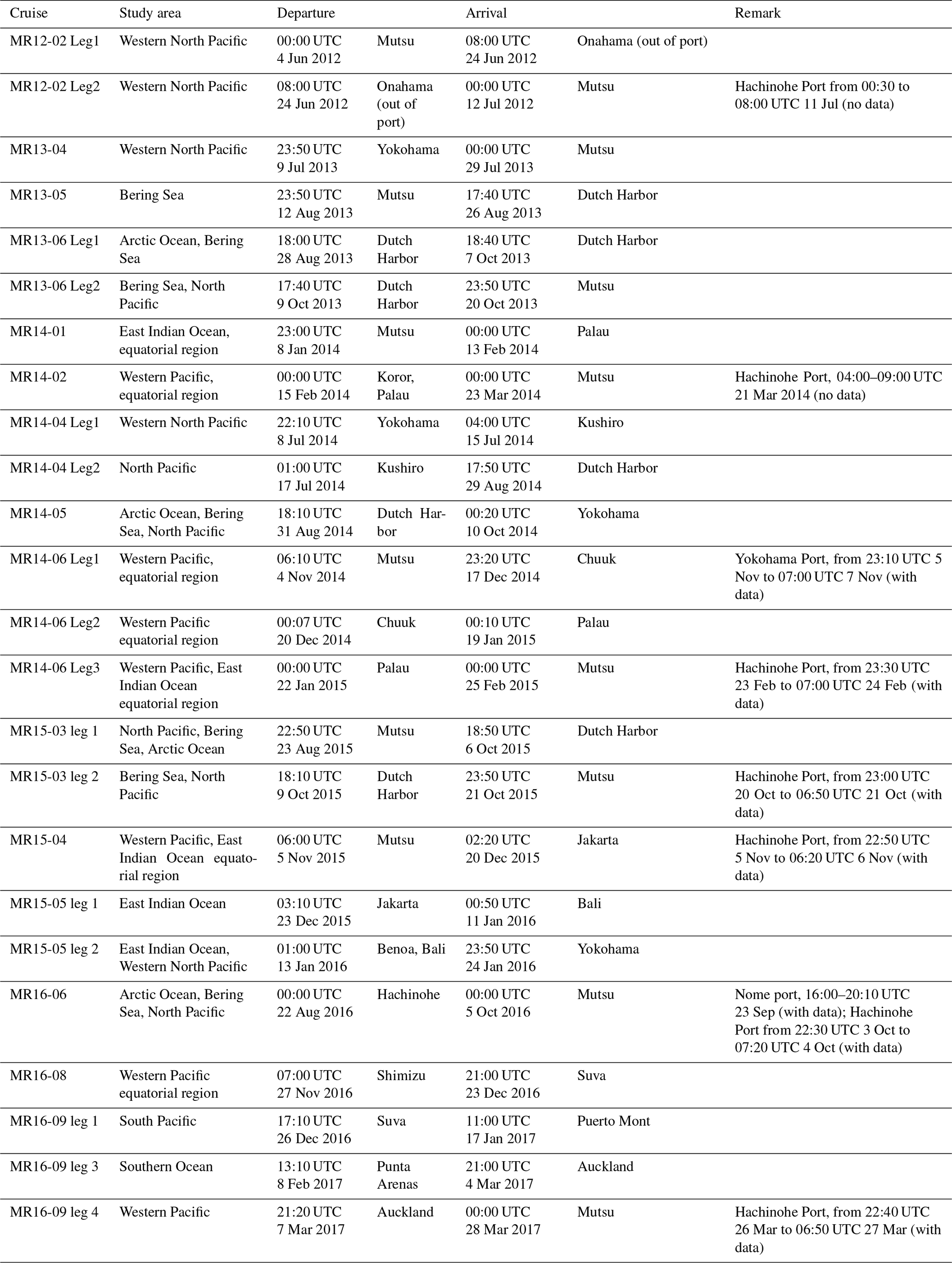
The 24 cruise legs during which the two instruments were operated are listed in Table 1. During MR12-02 Legs 1 and 2, the CO instrument did not work well and only the O₃ data were used for analysis. The cruise regions ranged widely, from the Arctic, the north, the Equator, South Pacific Ocean, and the eastern part of the Indian Ocean to the Southern Ocean. The Arctic cruises took place every year during the period 2013 to 2016 (specifically during the MR13-06, 14-05, 15-03, and 16-06 cruises). Other cruises aimed to study geology, meteorology, and oceanography and took place in the Pacific, Indian, and Southern oceans. The western Pacific equatorial region and Indian oceans were also frequently visited for operation of the TRITON buoy. Regions near Japan were frequently observed because the departure and arrival ports were often in that country. Our data basically did not include observations made while the vessel was anchored in ports; exceptions were the inclusion of short on-port data when the ports were visited during cruise legs (see the far-right-hand column in Table 1). During many cruises, other instruments, i.e., for performing black carbon and fluorescent aerosol measurements, and multi-axis differential optical absorption spectroscopy (MAX-DOAS), were operated together (e.g., Taketani et al., 2016; Takashima et al., 2016). These data will be reported in future publications.

Table 1 Overview of cruise legs of R/V Mirai used in this study.

2.2 Reanalysis and ACCMIP models

The first version of tropospheric chemistry reanalysis from JAMSTEC, i.e., TCR-1, which used an ensemble Kalman filter (EnKF) approach with a global atmospheric chemistry model (CHASER) as a base forward model, has been previously described (Miyazaki et al., 2015). Here, the updated version, TCR-2, was used (Miyazaki et al., 2019, https://ebcrpa.jamstec.go.jp/tcr2/about_data.html, last acces: 27 May 2019). The detailed description of the basic data assimilation framework and the evaluation results using the KORUS-AQ aircraft measurements over east Asia are available in Miyazaki et al. (2019), while detailed global evaluations are ongoing. The major aspects of the update of TCR-1 were a finer horizontal resolution (1.1^∘, compared with 2.8^∘ in TCR-1), assimilation of newer satellite data products – OMI NO₂ (QA4ECV), GOME-2 NO₂ (TM4NO2A v2.3), TES O₃ (v6), MOPITT CO (v7 NIR), and MLS O₃, HNO₃ (v4.2) – and extension of the period to 2017 (from 2005). A priori emissions were obtained from EDGAR v4.2 for anthropogenic sources, GFED v3.1 for open-fire emissions, and GEIA for biogenic sources. In addition to concentration fields of chemical species, NO_x emissions (surface and lightning, separately) and CO were included in the state vector and were simultaneously optimized. An advantage was that analysis for recent years (e.g., 2017) was possible before development of a bottom-up emission inventory. The base forward model CHASER V4.0 used for TCR-2 has been described by Sekiya et al. (2018). Briefly, 93 species and 263 reactions (including heterogeneous reactions) represent ${\mathrm{O}}_x-{\mathrm{NO}}_x-{\mathrm{HO}}_x-{\mathrm{CH}}_{\mathrm{4}}-\mathrm{CO}$ photochemistry and oxidation of nonmethane volatile organic compounds. Tropospheric halogen chemistry is not included. The dry deposition velocity (v_d) of O₃ was computed as ($r_{\mathrm{a}}+r_b+r_{\mathrm{s}}{)}^{-\mathrm{1}}$, where r_a, r_b, and r_s are the aerodynamic resistance, the surface canopy (quasi-laminar) layer resistance, and the surface resistance, respectively (Wesely, 1989). 1∕r_s over ocean surface was assumed to be 0.075 cm s⁻¹ globally, irrespective of region (Sudo et al., 2002). As a result, v_d was ∼0.04 cm s⁻¹ over the Arctic open ocean in September, for instance. This will be a subject of discussion in Sect. 3.3.2.

Because the number of assimilated TES O₃ retrievals decreased substantially after 2010, the data assimilation performance became worse after 2010 in the previous version TCR-1 (Miyazaki et al., 2015), and it can be expected that TCR-2 has similar increases in O₃ analysis errors after 2010. Nevertheless, the multi-constituent data assimilation framework provides comprehensive constraints on the chemical system and entire tropospheric O₃ profiles through corrections made to precursors' emissions and stratospheric concentrations, as demonstrated by Miyazaki et al. (2015, 2019).

We also used the monthly ACCMIP ensemble simulations for the present day (Shindell et al., 2011), which were represented as simulation results for a decade from 2000 (Stevenson et al., 2013; Young et al., 2013). The monthly mean O₃ field from an ensemble member, MIROC-Chem, with a modeling framework similar to that of TCR-2, provided corresponding climatological mixing ratio levels at a given location. These values were used to evaluate the performance of TCR-2, which uses meteorological data and estimated emissions in those particular years. Seven other ACCMIP ensemble members that provide hourly O₃ mixing ratios at the Earth's surface (CESM-CAM-superfast, CMAM, GEOSCCM, GFDL-AM3, GISS-E2-R, MOCAGE, and UM-CAM) were also used for comparative analysis in terms of frequency distribution of O₃ mixing ratios in the Arctic region (domain 1, 72.5–77.5^∘ N, 190–205^∘ E) and in a narrow western Pacific equatorial region (domain 3, 0–15^∘ N, 150–165^∘ E). The ACCMIP results were chosen for the latest intercomparison exercises because the data were publicly available.

2.3 Backward trajectory

Five-day backward trajectories from an altitude of 500 m above sea level (a.s.l.) were calculated every hour from the position of R/V Mirai by using NOAA's Hybrid Single-Particle Lagrangian Integrated Trajectory (HYSPLIT) model (Draxler and Rolph, 2013) to trace the origin areas of the observed air masses. GDAS1 three-dimensional meteorological field data with a resolution of 1.0^∘ were used. Cases that did not involve traveling over land regions (at altitudes lower than 2500 m a.s.l.) during the 5 days were extracted as marine air mass cases. Here, the land mask data from NASA (https://ldas.gsfc.nasa.gov/gldas/data/0.25deg/landmask_mod44w_025.asc, last access: 27 May 2019) at a resolution of 0.25^∘ were used for making judgments.

3 Results and discussion

3.1 Overview of geographical distributions of O₃ and CO

Figure 1a shows the entire O₃ data set from observations on R/V Mirai from 2012 to 2017. The covered latitudinal range was wide, from 67.00^∘ S (at 06:00 UTC on 16 February 2017 during MR16-09 Leg 3) to 75.12^∘ N (at 06:00 UTC on 6 September 2014 during MR14-05). The highest hourly mixing ratio, i.e. 66.6 ppbv, was recorded twice: first at 35.89^∘ N, 141.95^∘ E, about 70 km east off the coast of the Kanto area, Japan, at 04:00 UTC on 6 July 2012, and second at 32.29^∘ N, 146.04^∘ E, about 500 km southeast of the Kanto area at 14:00 UTC on 18 March 2014. During 57 h, the hourly values exceeded 60 ppbv (which corresponds to the environmental standard in Japan) in a similar region off the coast of Japan, under the influence of Asian regional air pollution. The lowest hourly mixing ratio, i.e. 4.3 ppbv, was recorded twice on the western Pacific equatorial region: first at 5.86^∘ N, 156.00^∘ E and secondly at 7.96^∘ N, 156.02^∘ E at 09:00 and 21:00 UTC, respectively, on 11 March 2014. Values lower than 10 ppbv were recorded for a total of 800 h; this will be discussed in the following section.

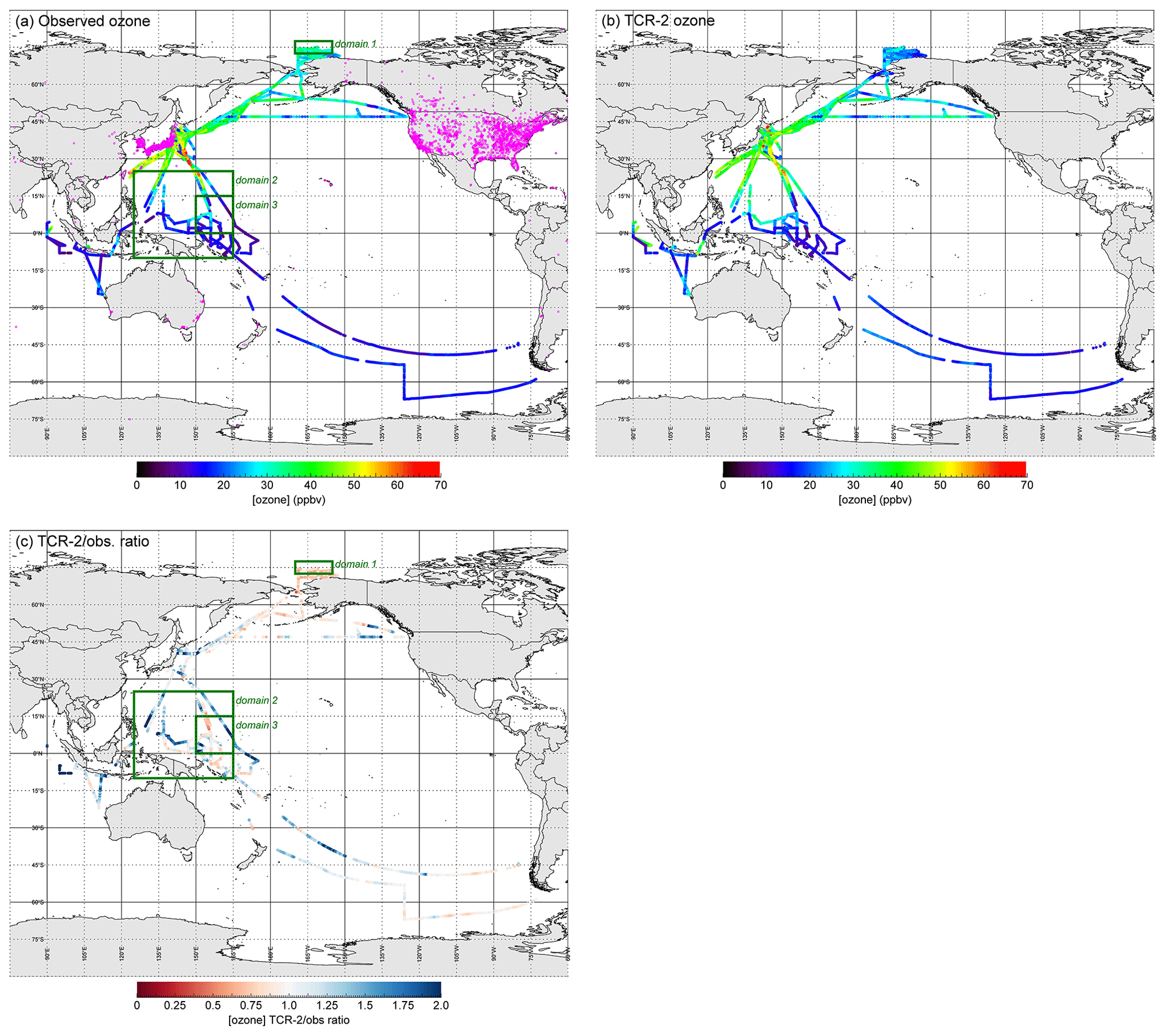
Figure 1 Geographical distributions from (a) observed hourly O₃ mixing ratios (N= 11 666) on R/V Mirai during 24 research cruise legs in 2012–2017 and (b) those from reanalysis (TCR-2) of data along R/V Mirai cruise track; (c) reanalysis∕observation ratios (TCR-2/obs) for O₃ mixing ratios. In (a) stationary points of TOAR data set are plotted (magenta dots). In (a) and (c), three green rectangles show focused domains in the Arctic (domain 1, 72.5–77.5^∘ N, 190–205^∘ E) and two in the western Pacific equatorial region (domain 2, 10^∘ S to 25^∘ N, 125–165^∘ E; domain 3, 0–15^∘ N, 150–165^∘ E).

Figure 2a shows the entire CO data set. The highest mixing ratio was 556 ppbv, which was recorded at 58.00^∘ N, 179.23^∘ E, at 01:00 UTC on 26 September 2016 during the MR16-06 cruise, where a dense plume from severe forest fires in Russia reached as far as the Bering Sea. All 8 h in which the mixing ratio exceeded 500 ppbv were recorded on the same day. There were 59 other hours when the CO mixing ratio exceeded 300 ppbv, when anthropogenic emissions from east Asia and/or biomass burning were important.

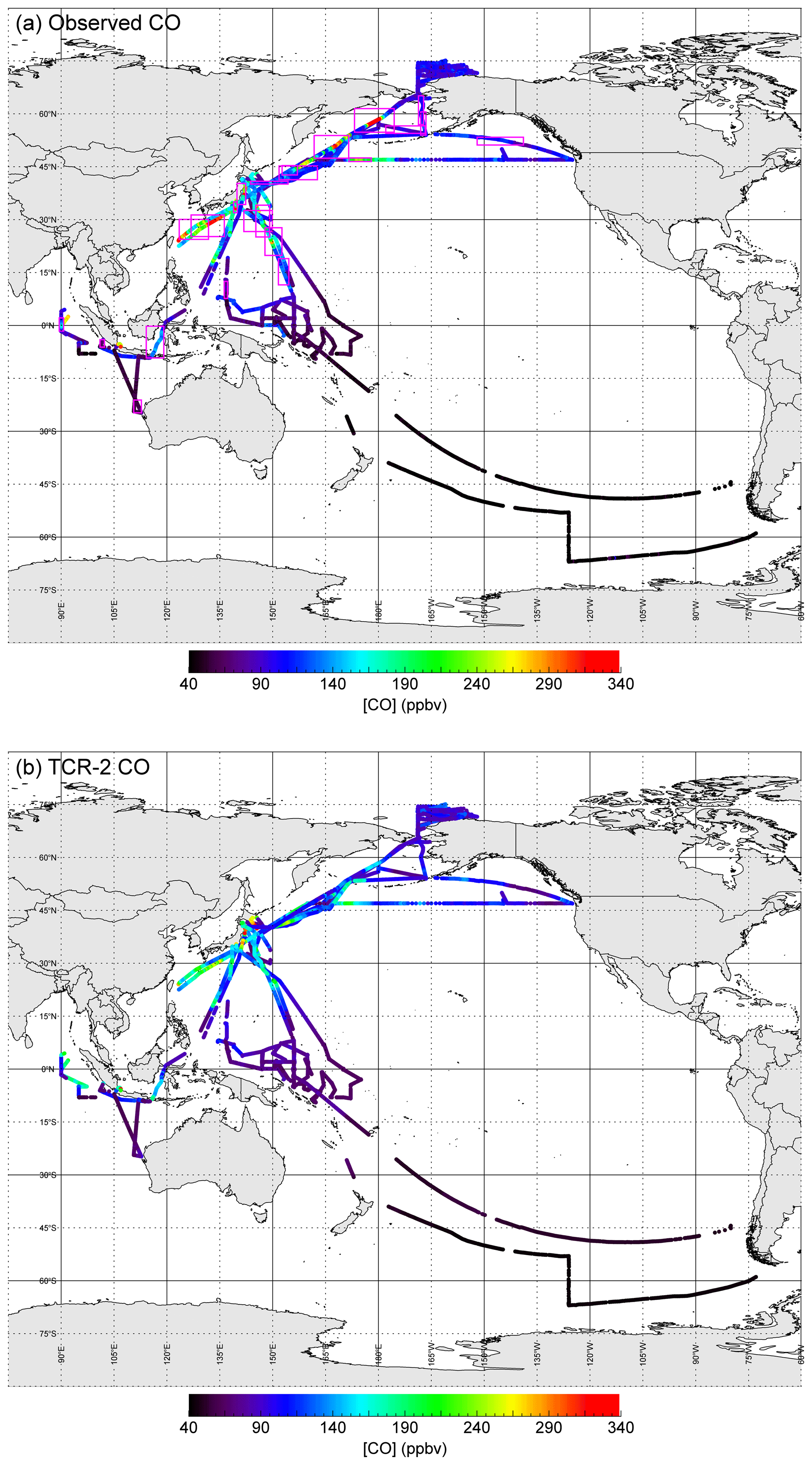
Figure 2 Geographical distributions of (a) observed CO mixing ratios and (b) those from TCR-2. In (a) magenta boxes indicate 23 regions where ΔO₃∕ΔCO ratios were analyzed (see Fig. 8 and Table 2).

Figure 3 shows an example of O₃ variations for data from MR14-06 Leg 1 with backward trajectories. The vessel started from Mutsu port (41.37^∘ N, 141.24^∘ E), stayed for about 32 h at Yokohama port (35.45^∘ N, 139.66^∘ E), and then headed to the western Pacific equatorial region. A latitudinal gradient was apparent: north of 27^∘ N was dominated by air masses originating from the Asian continent, as shown by violet trajectory lines. During some hours, high levels, i.e., greater than 50 ppbv of O₃, were recorded (points with red trajectory lines). In contrast, marine air masses from the east were dominant south of 27^∘ N and the mixing ratio levels decreased to less than 30 ppbv. South of 15^∘ N, even lower levels were dominant, i.e., < 15 ppbv, particularly in equatorial regions where levels less than 10 ppbv of O₃ were frequently observed. The latitudinal gradient, air mass exchange, and transport of photochemically produced O₃ are the three important factors determining distributions. Figure S1 in the Supplement shows the spatial distributions of O₃ and backward trajectories for each cruise leg, and their time series. All three factors listed above for the MR14-06 Leg 1 had major effects on the variations. The classification of air masses as marine and other cases was satisfactory for identifying cases of long-range transport of pollutants from continents, although some events with continental effects with traveling times longer than 120 h were probably wrongly categorized. Because longer trajectories may not be reliable, we will use this criterion (i.e., 120 h) in the following sections with a notice of such limitations. Stratospheric influences were not identified: we did not find any events with reasonable O₃-level enhancement accompanied by descent of air masses from 8 km or higher altitudes within 72 h prior to observations.

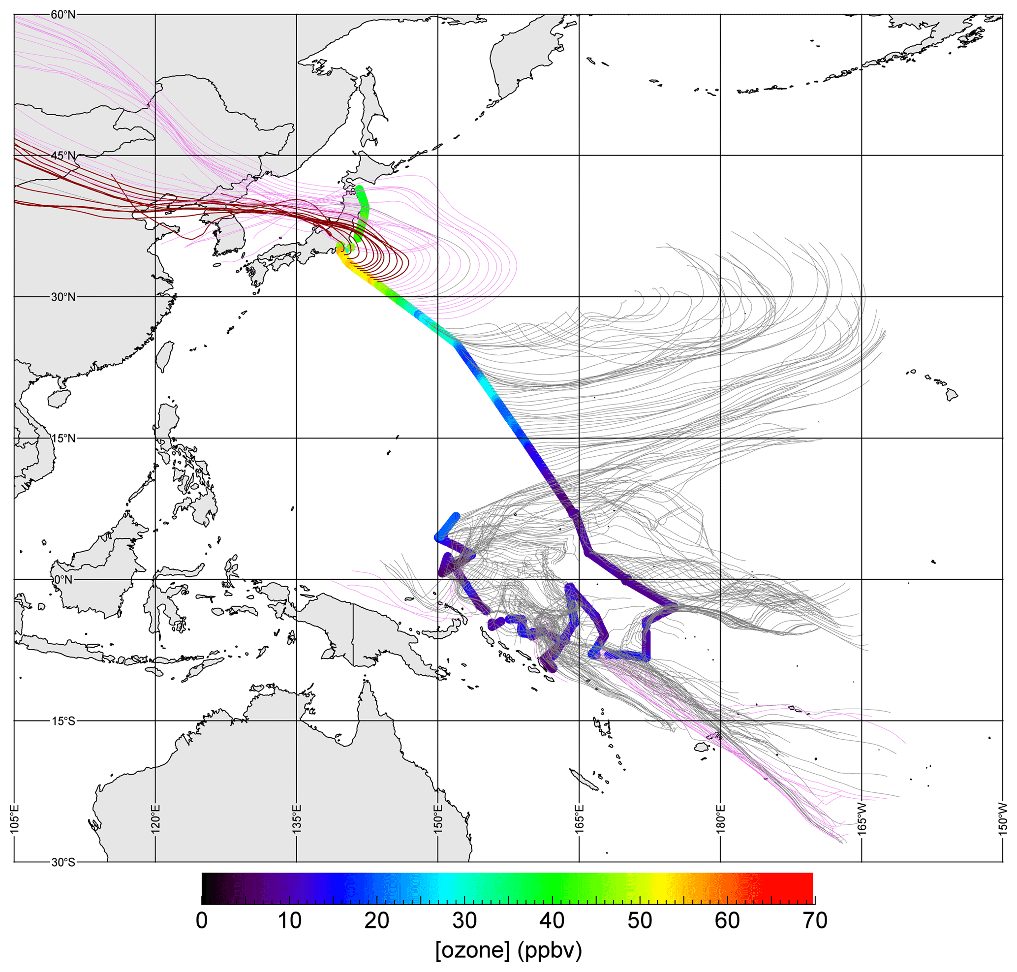
Figure 3 Observed O₃ mixing ratios during MR14-06 Leg 1 and backward trajectories (120 h). Magenta lines indicate cases in which trajectory entered regions over land (at altitudes < 2500 m a.s.l.). Red lines indicate cases in which observed O₃ mixing ratios exceeded 50 ppbv.

3.2 Comparisons between observations and TCR-2 data: Global features

Figures 1b and 2b show the geographical distributions of O₃ and CO obtained from TCR-2 along the cruise track. The nearest grid and time (2 h resolution) at the lowest layer were sampled to achieve the best possible comparison with the observations shown in Figs. 1a and 2a. Most features were in agreement with the observations, in terms of areas with high mixing ratios and latitudinal gradients. This comparison indicates a reasonably high quality of reanalysis data over the oceans. This is partly because the NO_x and CO emissions rates were optimally estimated during the data assimilation cycle and were reflected in the mixing ratio field. The emission changes provide substantial influences on ozone forecasts over many regions. Assimilation of the TES ozone measurements has limited impacts on near-surface ozone owing to its weak sensitivity to the lower troposphere.

In Fig. S1, the comparisons are shown as time-series plots. Excellent matches in the evolution with time of O₃ and CO mixing ratios were found for the latter period of MR14-02, i.e., during the period 12–22 March 2014, in the time series (Fig. S1g). The blue lines show plots of monthly climatological mean mixing ratios, which were obtained from MIROC-Chem. Although the monthly means sometimes followed the observed baseline trend for O₃, the performance of TCR-2 was superior, particularly for reproducing detailed peak patterns for CO. This case will be analyzed in Sect. 3.3.1 on photochemical buildup. A similarly excellent performance was obtained for MR15-05 Leg 2 (Fig. S1r) and MR16-09 Leg 4 (Fig. S1w), when the ship returned to Japan from the south.

Clear gaps were also sometimes observed. These are probably related to limited reproducibility in the meteorological field and errors in the emission estimation and other physicochemical processes that were taken into account in the model system. A large gap was observed during the latter half of the MR14-01 cruise (Fig. S1f); the predictions produced by TCR-2 for CO and O₃ in the eastern Indian Ocean were too high. The climatological mean from MIROC-Chem reproduced the observed level better, which suggests that false information was introduced from satellite observations to the surface mixing ratios, for instance, associated with the use of total column measurements and errors in vertical transport, or that the position of ITCZ was too far south in the simulation. During other cruises, smaller gaps in the peak occurrence times and peak mixing ratio levels were found. For example, during MR14-04 Leg 2 (Fig. S1i), the peak times for O₃ and CO during the period 27 July to 6 August 2014 were out of phase by about 1 to 2 days. This was probably caused by a small displacement of pollution air masses after long-range transport. High O₃ mixing ratios, i.e., > 70 ppbv (off the scale in the time-series plot) for 23 h were predicted by TCR-2, which was an overestimation compared with the observations. Except for 2 h on 9 October 2014, these were always in July (in 2012, 2013, and 2014). All were found within 200 km east of Japan's main islands, suggesting overestimation of photochemical O₃ production during long-range transport in TCR-2.

With such case-dependent reproducibility in mind, Fig. 1c summarizes the overall geographical distribution of the reanalysis∕observation ratios for O₃ mixing ratios. For clarity, the data were limited to cases of marine origins, where the differences between the TCR-predicted and -observed CO mixing ratios were less than 50 ppbv (N=5662), in contrast to Fig. 1a, b, where all data (N= 11 666) were included. The model's underestimation in the Arctic Ocean and overestimation over the oceans south of Japan (western Pacific equatorial or subtropical regions) are clearly shown. These features will be discussed in Sect. 3.3.

Figure 4 shows the latitudinal distribution of the observed and TCR-2 O₃ mixing ratios and their ratios. In Fig. 4a, the data were again limited to cases of marine origins, where the differences between the model-derived and observed CO mixing ratios were less than 50 ppbv (N=5662). The variability shown here reflects seasonality and cases of long-range transport from continents over 120 h. The range of TCR-2∕observation ratios (shown in red in Fig. 4b) narrowed when TCR-2 successfully captured the variability. Data selection (N=5662) also contributed to narrowing of the range (grey points indicate without data selection). The ratios binned by latitudes indicate that TCR-2 tended to give underestimations at high northern latitudes and overestimations at low latitudes. The 10th, 50th (median), and 90th percentiles (range shown as bars) of the ratios at high latitudes (> 70^∘ N) were 0.62, 0.81, and 0.94 (N=876); the range was off unity. The medians for low latitudes (0–10, 10–20, and 20–30^∘ N) were 1.12 (N=1061), 1.28 (N=268), and 1.28 (N=195), respectively.

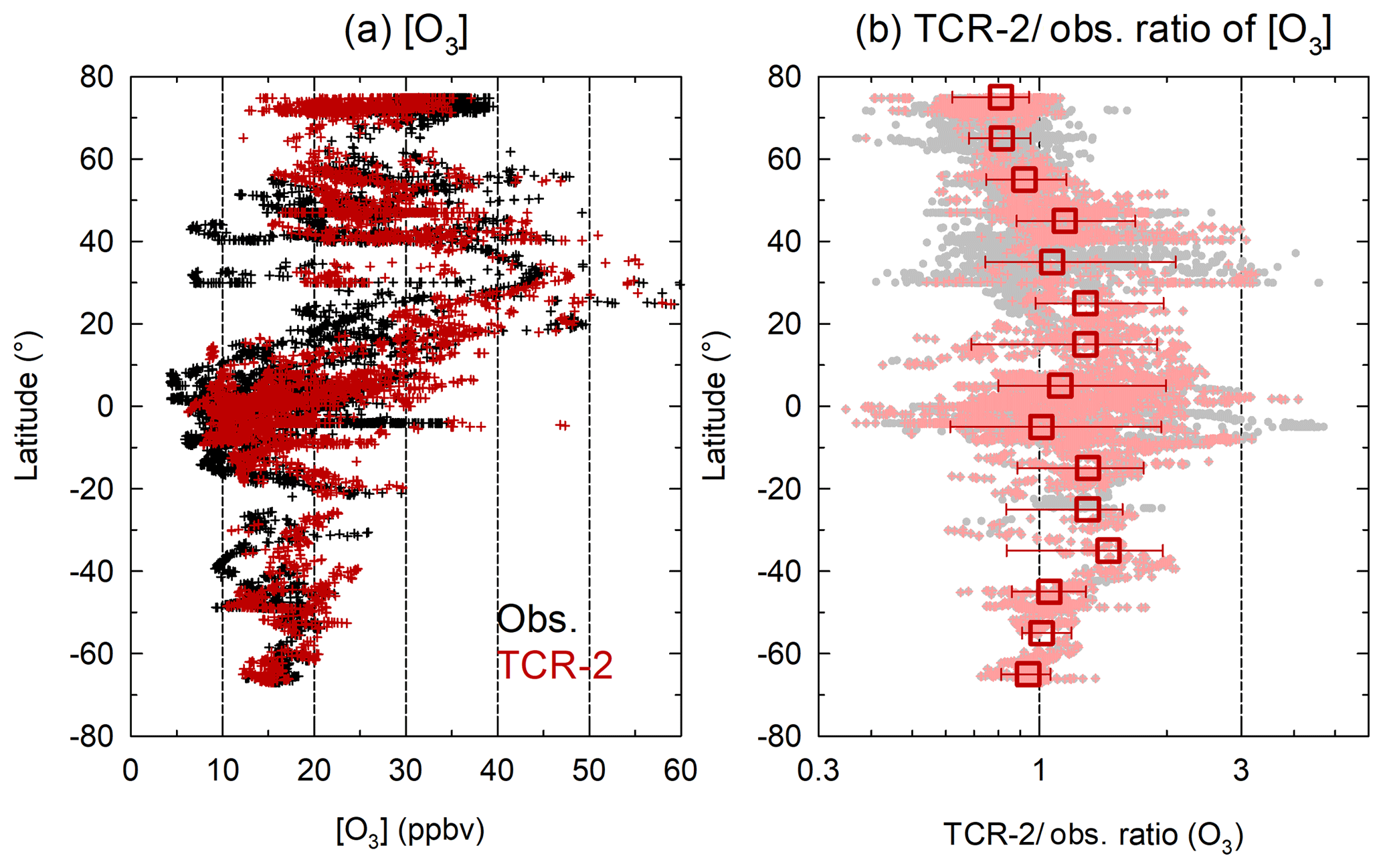
Figure 4 (a) Latitudinal distribution of O₃ mixing ratios from observation (black) and TCR-2 (red). Data are limited to cases of marine origins where difference between predicted and observed CO mixing ratios was less than 50 ppbv (N=5647). (b) Latitudinal distribution of TCR-2∕observation ratio for O₃ (light-red dots) and binned medians (ranges are from 10th to 90th percentile) over 10^∘. Gray dots represent all cases without data selection.

Figure 5 shows a scatterplot of the comparison. The data set was re-expanded by removing the criteria of marine air mass selection and CO differences (i.e., N= 11 666) to show the overall correlation between the observed and TCR-2 data over the full range. The square of the correlation coefficient (R²) was 0.59; this increased to 0.62 when clear outliers (latter half of MR14-01 and cases in which TCR-2 exceeded 70 ppbv) were omitted (red, N= 11 305). The excellent performance of TCR-2 was assured by a resolution of 2 h in reproducing O₃ mixing ratio variations. When the data were further binned to a resolution of 1 day (with observations for 6 h or more), R² improved to 0.66; this suggests that the original variability was partly derived from small shifts in the peak times by less than a day. In the past, reanalysis data were not used for such detailed diagnoses but were normally compared with observations after monthly averaging or binning to coarse latitudinal bands. Recently, Akritidis et al. (2018) evaluated stratosphere-to-troposphere transport processes represented by the Copernicus Atmosphere Monitoring Service (CAMS) system, but evaluation of transport and transformation processes for tropospheric O₃ over oceans has not been reported with reanalysis. Here, a successful comparison was made for the first time at the daily or finer timescale. The regression line for the data set, i.e., [TCR-2, ppbv] $=(\mathrm{6.90}\pm \mathrm{0.15})+(\mathrm{0.71}\pm \mathrm{0.01})\times$ [obs, ppbv], suggests a statistically significant positive intercept on the y axis (i.e., TCR-2) and a slope of less than unity. The result was unchanged even when MR14-01 and cases with > 70 ppbv in TCR-2 were included. The green circles in Fig. 5 represent data from the Arctic region (> 70^∘ N) and clearly suggest an underestimation by TCR-2. In contrast, the blue circles from the western Pacific equatorial region (125–165^∘ E, 10^∘ S to 25^∘ N) fell on the opposite side, with respect to the 1:1 line, indicating an overestimation by TCR-2. These two aspects will be discussed in detail in the following sections.

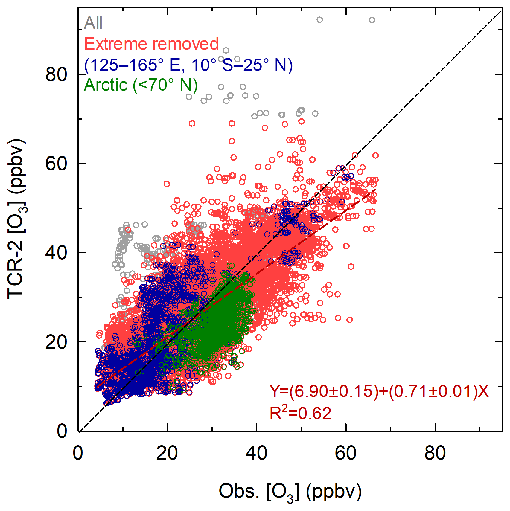
Figure 5 Scatterplot of observed and reanalysis O₃ mixing ratios. Gray circles include all data (N= 11 666), red circles are cases in which data from MR14-01 and extreme cases in which TCR-2 exceeded 70 ppbv were removed. Green circles indicate data from Arctic region (> 70^∘ N) and blue circles indicate data from domain 2 (125–165^∘ E, 10^∘ S to 25^∘ N).

3.3 Specific analysis with event or regional focuses: Implications for processes

In this section, more detailed comparisons between observations and simulations are made to shed light on the underlying mechanisms determining O₃ mixing ratio levels and distributions.

3.3.1 Long-range transport events with photochemical production

We selected events with simultaneous increases in CO and O₃ levels or those with at least evident CO peaks. We then assessed the reproducibility of the peak mixing ratios and ΔO₃∕ΔCO ratios in TCR-2; the ΔO₃∕ΔCO ratio is an index of the efficiency of photochemical production of O₃ from CO as a precursor. In total, 23 cases were selected (Table 2 and magenta rectangles in Fig. 2a). The two cases discussed below were studied in depth.

Table 2 Cases of long-range transport events used for examination of photochemistry (unit for ΔO₃∕ΔCO is ppbv/ppbv).

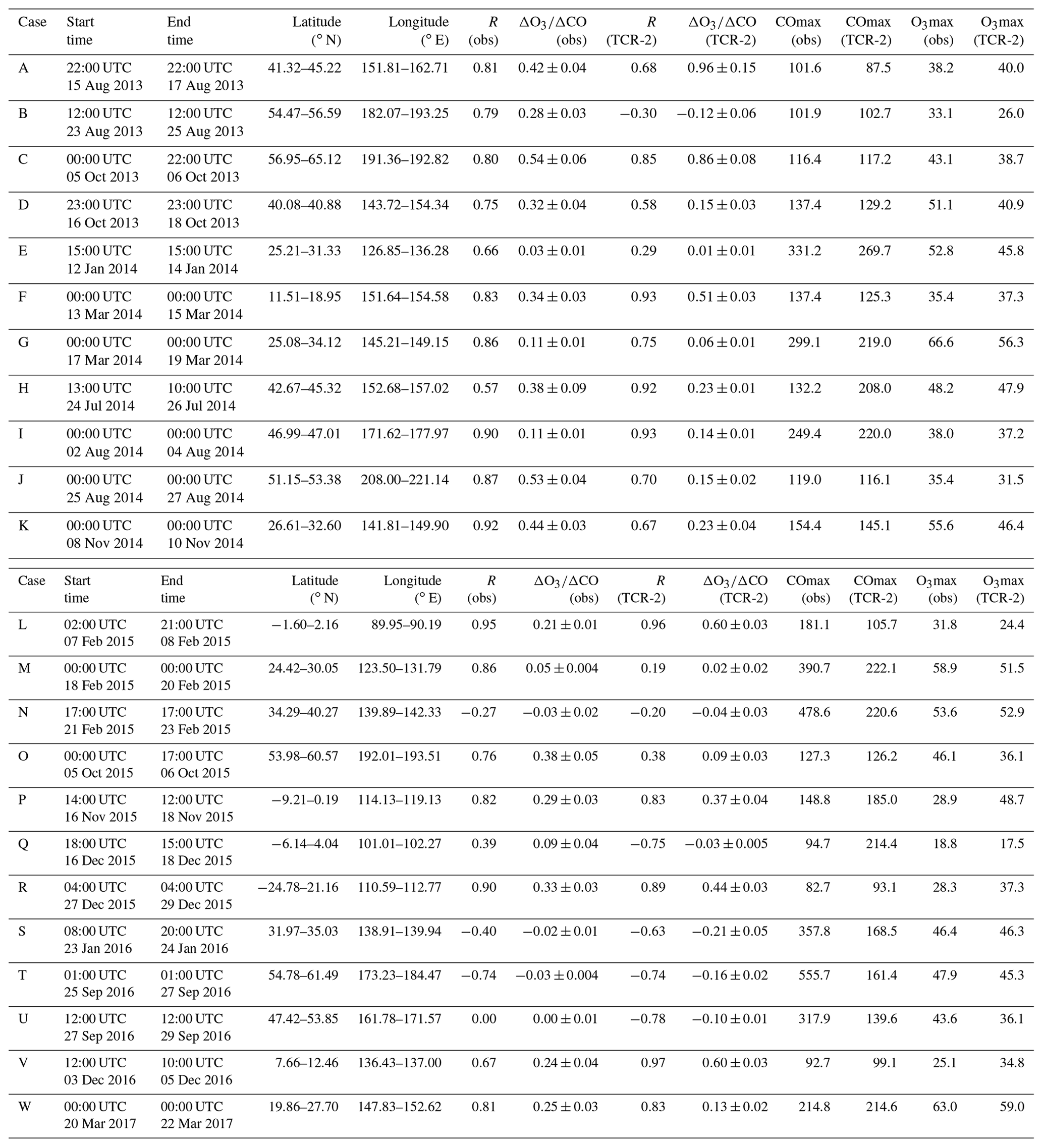
Figure 6 Temporal evolution of surface CO and O₃ distribution from TCR-2 (colored open squares) and from observations on R/V Mirai (all data, position of vessel is black circle) during MR14-02 (from 16 to 19 March 2014). Black circles in the bottom-left CO panel indicate locations with high anthropogenic CO emissions (EDGAR).

Figure 6 shows the time evolution of the O₃ and CO mixing ratios from observations and TCR-2 during the period 16–19 March 2014, when the vessel returned to Japan from the equatorial Pacific during MR14-02. The observational data along the entire track are shown, with the exact position of R/V Mirai at that time marked by a black circle. This part of the cruise has already been briefly mentioned in Sect. 3.2; here, the origins of pollution and the photochemical states for three episodes with increased mixing ratios are discussed. First, at 09:00 UTC on 16 March 2014, at 23.69^∘ N, 149.72^∘ E, the CO mixing ratio peaked at around 284 ppbv. The geographical distribution of surface O₃ and CO in TCR-2 implied that this was a tongue-shaped pollution event originating from mainland southeast Asia (formerly the Indochina Peninsula) and extending to the east; however, it was not. Instead, as inferred from the backward trajectories (Fig. S1g), weather charts, and time evolution of CO distributions from TCR-2 (Fig. 6), it should be interpreted as a belt of pollution originating from east Asia, present at the south edge of a high-pressure system moving toward the southeast. An O₃ peak of 54.2 ppbv occurred 10 h later, which was also captured by TCR-2. A second CO peak occurred the next day, at 19:00 UTC on 17 March 2014, at 28.56^∘ N, 147.68^∘ E; in this case an O₃ peak of 66.2 ppbv occurred just 1 h before. TCR-2 suggested that the plume originated from east Asia and was transported to the east from the continent and then to the south, under the influence of another high-pressure system traveling over Japan and a low-pressure system that followed (see the second row panel in Fig. 6 for 01:00 UTC on 17 March 2014). The timing and location of the third peak were also well predicted; a CO peak of 273 ppbv occurred at 17:00 UTC on 18 March 2014, at 32.88^∘ N, 145.77^∘ E, 3 h after the O₃ peak of 66.6 ppbv (the highest in the data set). In this case, the air mass traveled directly from central east China, with a large precursor emission (see the distribution of grids with high CO emissions in the panel for 01:00 UTC on 19 March 2014) via a quick westerly flow under the influence of passage of a cold front. The ΔO₃∕ΔCO ratio, calculated as the slope of the regression line in a scatterplot of hourly mixing ratios of O₃ and CO between 00:00 UTC on 17 March 2014 and 00:00 UTC 19 on March 2014, was 0.11±0.01 ppbv/ppbv (R=0.83) for observations and 0.06±0.01 ppbv/ppbv (R=0.75) for TCR-2 (Table 2, case G). The underestimation of O₃ peaks by TCR-2 (maximum 56.3 ppbv) is attributable to a combination of less efficient production of O₃ and underestimation of CO peaks by TCR-2 (maximum 219 ppbv).

Figure 7 shows a similar time evolution during MR14-04 Leg 2, when a plume reached the central Pacific from the Asian continent about 5000 km away. The ΔO₃∕ΔCO ratio from 00:00 UTC on 2 August 2014 to 00:00 UTC on 4 August 2014 was 0.11±0.01 ppbv/ppbv (R=0.90) for observations and 0.14±0.01 ppbv/ppbv (R=0.93) for TCR-2. The maximum CO and O₃ mixing ratios were 249 and 38.0 ppbv, respectively, for observations, and 220 and 37.2 ppbv, respectively, for TCR-2 (Table 2, case I). The pollution source was probably forest fires in the far east of Russia (shown by plus signs in the upper-left panel of Fig. 7) with a smaller contribution from anthropogenic emissions from east Asia. Specifically, on 26 July 2014, the head of a plume extending from the forest fires arrived in northern Japan (see Zhu et al., 2019 and references therein for details) and affected our ship observations. The main body of the plume arrived from the west and traveled with a migrating high-pressure system until 6 August 2014. The observed CO and O₃ mixing ratios decreased during the period 29 July to 1 August 2014, when the vessel was located at the center of a low-pressure system traveling to the east. After the low-pressure system had weakened, the plume was still present in its southern part and was pushed northeast under the influence of the high-pressure system in the south, which again affected the ship observations during 2 and 3 August 2014, in the middle of the North Pacific.

Figure 7 Temporal evolution of surface CO and O₃ distribution from TCR-2 (colored open squares) and from observations on R/V Mirai (all data; position of vessel is shown by black circle) during MR14-04 Leg 2 (from 26 July to 3 August 2014). Plus signs in the top-left panel show points with high carbon emissions from wildfires (GFED).

Table 2 summarizes the results from all 23 cases, including the two events discussed above (cases F and G from MR14-02 and cases H and I from MR14-04 Leg 2). The span of the study area was from the Indian Ocean in the Southern Hemisphere, and the central equatorial Pacific Ocean to the Bering Sea (see magenta rectangles in Fig. 2a). In most cases, the observed ΔO₃∕ΔCO slopes were positive, suggesting photochemical buildup of O₃ with emissions of CO. The ranges were well reproduced by TCR-2. It is interesting to note that negative slopes for ΔO₃∕ΔCO were found for at least three cases and that these were also well captured by TCR-2. These were the cases where very high CO levels were recorded (479, 358, and 556 ppbv for cases N, S, and T, respectively). The strong negative correlation for case N was influenced by the low O₃ mixing ratios (11.2 ppbv) recorded with high CO levels. When such irregular points were removed, the observed slope was 0.01±0.01 ppbv/ppbv. For case S, a strong CO peak occurred in the south of Japan (∼200 km off the coast) on 23 January 2016, without an O₃ increase (Fig. S1r). For case T, a plume from a Russian forest fire affected the observations over the Bering Sea (Fig. S1s). Relatively fresh air pollution from nearby ships or weak UV in January and February for cases N and S, and weak co-emission of NO_x from forest fires for case T, could cause the observed negative slopes. Processes other than daytime photochemistry (e.g., nocturnal chemistry) might also have been important.

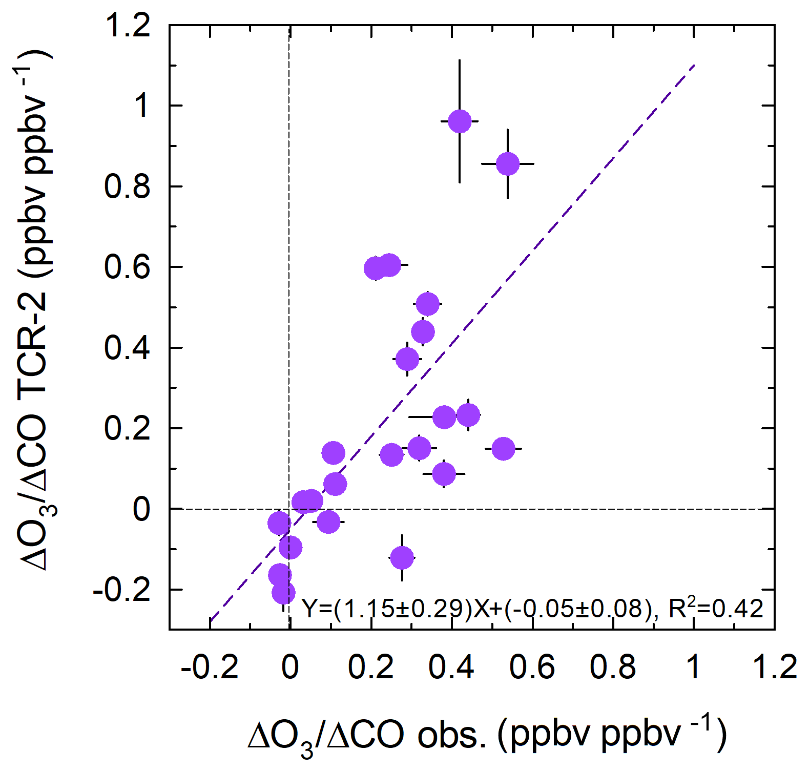
Figure 8 shows the correlation between the observed and reanalysis ΔO₃∕ΔCO ratios. The reasonable correlation, with a slope of 1.15±0.29 and R²=0.42, suggests that TCR-2 reproduced the state of O₃ production fairly well for various cases in different geographical domains in different seasons. Case B is an outlier in terms of correlation: observations and TCR-2 yielded ΔO₃∕ΔCO ratios of 0.28±0.03 and $-\mathrm{0.12}\pm \mathrm{0.06}$ ppbv/ppbv, respectively. This was recorded at the center of the Bering Sea, where TCR-2 failed to reproduce the coinciding increases in the observed O₃ and CO mixing ratios.

Figure 8 Correlations between ΔO₃∕ΔCO ratios from observations and TCR-2.

The observed and simulated ranges of the ΔO₃∕ΔCO ratios are in accordance with previously reported data. On the Azores in the central Atlantic (38.73^∘ N) in spring and on Sable Island (43.93^∘ N) in Atlantic Canada in summer, the ΔO₃∕ΔCO ratios were uniform, at 0.3–0.4 ppbv/ppbv (Parrish et al., 1998). For TRACE-P aircraft measurements, Hsu et al. (2004) reported smaller values, i.e., 0.08 ppbv/ppbv in the tropics and 0.03 ppbv/ppbv in the extratropics, with CO > 200 ppbv. Weiss-Penzias et al. (2006) reported 0.22 ppbv/ppbv in April and May 2004 for two long-range transport events that reached a mountain on the west coast of the United States from Asia. Tanimoto et al. (2008) summarized the range as being from slightly negative to ∼0.4 ppbv/ppbv when observing Siberian fire plumes at Rishiri Island. Zhang et al. (2018) documented the ΔO₃∕ΔCO ratios at Pico Mountain in the Atlantic Ocean and found that the ratios for anthropogenic pollution were higher (0.45–0.71 ppbv/ppbv) than those for observations affected by wildfires (0.12–0.71 ppbv/ppbv). They suggested that the low ratios from wildfires could be the result of lower NO_x∕CO emission ratios compared with those for anthropogenic sources.

3.3.2 Arctic processes

In the Arctic Ocean (> 70^∘ N), the CO mixing ratios were regularly close to the background and stable (101±10 ppbv, Fig. S1d, j, n, and s), suggesting that the measurements were not affected by strong pollution events. The average observed O₃ mixing ratio was 31.3 ppbv (N=1804) and the reanalysis significantly underestimated this (24.6 ppbv) based on Welch's t test (p< 0.001). The magnitude of the relationship was common for all 4 years of measurements (Fig. 9). A low bias with TCR-2 was also clear for cumulative frequency distributions of hourly O₃ mixing ratios from observations (black, N=1031) and TCR-2 (red) in domain 1 (72.5–77.5^∘ N, 190–205^∘ E) in September (Fig. 10). The frequency distributions for eight model members of ACCMIP and their ensemble median (magenta) are also included in Fig. 10. The median was close to that for TCR-2 and similarly significantly underestimated, although three members (GEOSCCM, GFDL-AM3, and GISS-E2-R) showed better agreement with observations. These analyses suggest that, in the simulations, the sources were too weak or the losses were too strong. The average diurnal variations were generally almost flat (the variability was within 5 % of the average) for observations and TCR-2 (not shown), suggesting that the missing processes did not show significant diurnal variability. At high latitudes, the assimilated measurements have either low quality or low sensitivity in the troposphere, while the optimization of precursors emissions generally has limited impacts on ozone. The reanalysis ozone over the Arctic Ocean can be similar to the model predictions, except when poleward transports are strong enough to propagate observational information from low latitudes and midlatitudes.

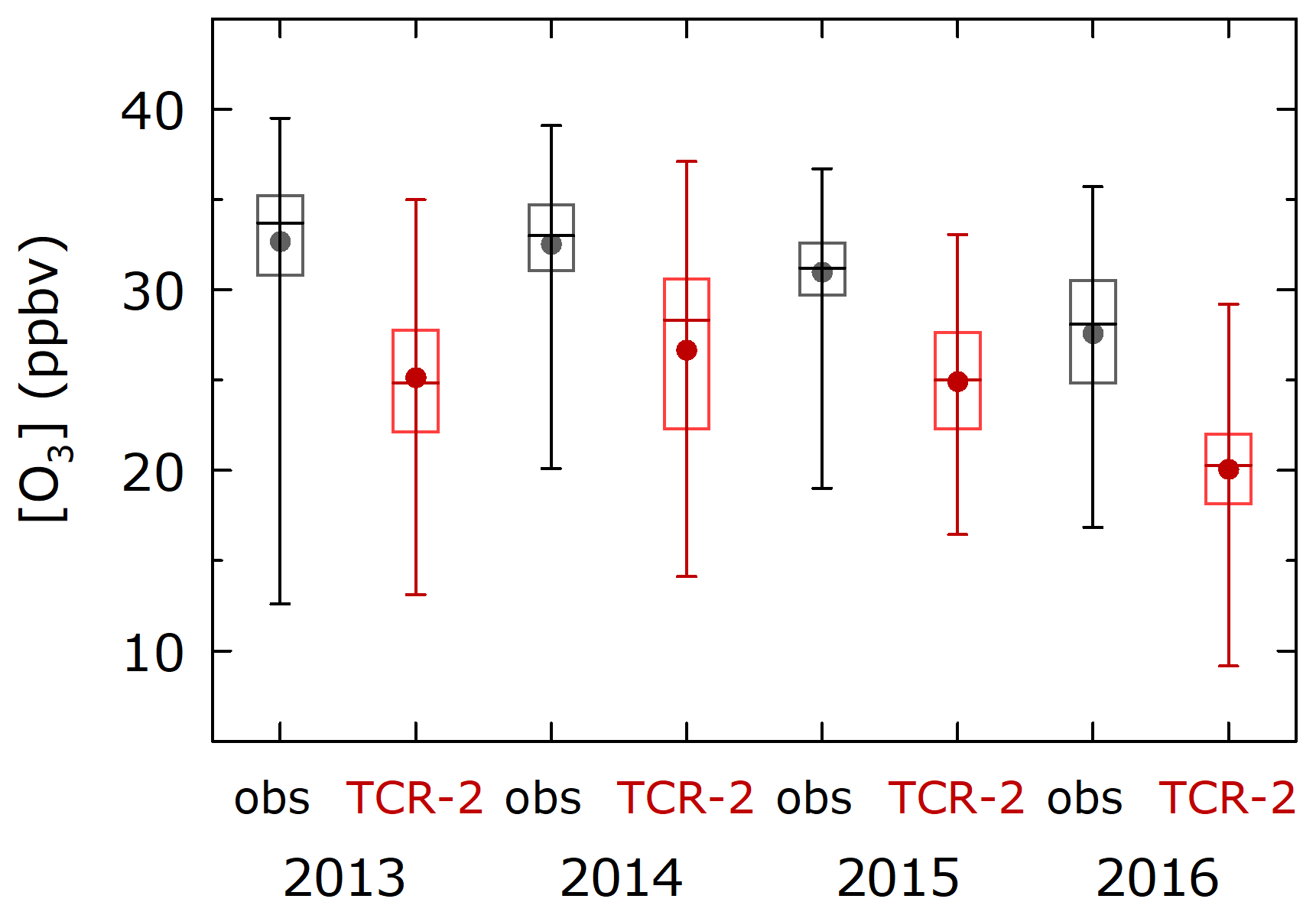
Figure 9 Repeated underestimations of O₃ mixing ratios ranges by TCR-2 relative to observed values in the Arctic region (> 70^∘ N). Boxes and horizontal bars indicate 75 %, 50 % (median), and 25 %, and whiskers indicate 90 % and 10 %. Circles are averages.

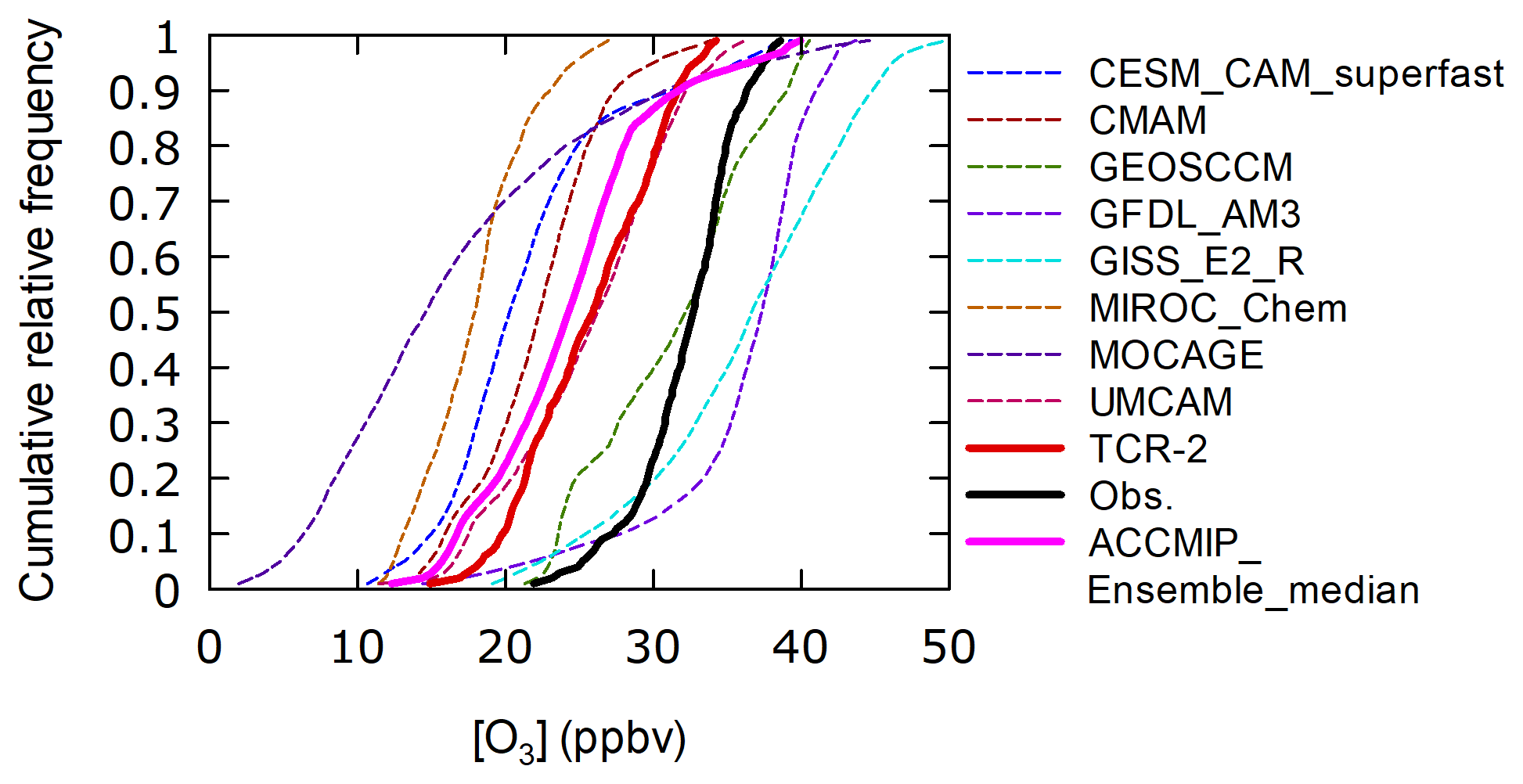
Figure 10 Cumulative relative frequency distributions of O₃ mixing ratios from observations (black), TCR-2 (red), and members and ensemble median of ACCMIP in the Arctic grid 1 (72.5–77.5^∘ N, 190–205^∘ E) in September.

During the MR14-05 cruise, 10 O₃ sondes were launched every other day at 22:00 UTC during the period 6–24 September 2014 (Inoue et al., 2018). The average vertical profile was compared with that from TCR-2 at the nearest grid (Fig. 11) to investigate the altitude to which this low bias of TCR-2 continued. At the lowest altitude near the surface, the underestimation by TCR-2 against the O₃ sonde observations was evident. However, the gap only continued to about 850 hPa, at which the two mixing ratios crossed over, and TCR-2 gave higher mixing ratios at higher altitudes. This suggests that the missing process was only important for the boundary layer, not for the entire troposphere. Inoue et al. (2018) compared the O₃ sonde profiles with ERA-Interim (ERA-I) products, with a focus on troposphere–stratosphere exchange. They found that in the upper-troposphere ERA-I had a high bias against observations, similarly to the case for TCR-2; this confirms that the underestimation by the model for the surface did not continue into the tropopause. One possibility is that the model's vertical (downward) mixing near the top of the boundary layer was too weak: this mixing would otherwise have effectively carried the O₃-rich air mass from higher altitudes. Another possibility is that dry deposition on the surface of the Arctic Ocean by the model was too fast. The v_d, ∼0.04 cm s⁻¹ over the Arctic open ocean in September for CHASER (TCR-2), is on the high side of ∼0.01–0.05 cm s⁻¹, a range adopted into global atmospheric chemistry models (see Fig. 4 of Hardacre et al., 2015). Ganzeveld et al. (2009) discussed a sensitivity model run, shifting their standard v_d of 0.05 to 0.01 cm s⁻¹, which substantially increased surface ozone concentrations by up to 60% in high-latitude regions.

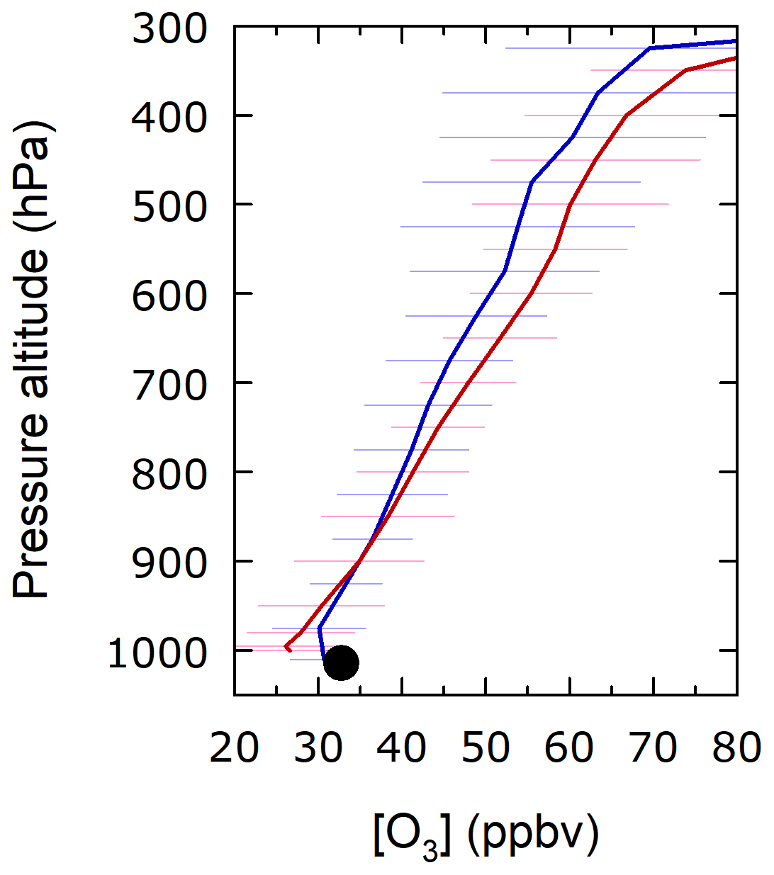
Figure 11 Average profile from O₃ soundings (blue) and that from TCR-2 (red). Average from surface observations on R/V Mirai is shown as black circle.

At Barrow (71.32^∘ N, 156.6^∘ W), the nearest ground-based site, the monthly average O₃ mixing ratios in September were 29.8 and 29.1 ppbv, in 2013 and 2014, respectively (McClure-Begley et al., 2014). These values are close to our observations over oceans, and the model ensemble tended to underestimate mixing ratios in September (AMAP, 2015), similarly to our case.

3.3.3 O₃ levels below 10 ppbv at low latitudes

Figures 1c, 4, and 5 show that TCR-2 tended to overestimate O₃ mixing ratios over the western Pacific equatorial region. For the whole global data set, TCR-2 predicted O₃ levels below 10 ppbv O₃ during 262 h, which is much less than the observed duration, i.e., 800 h. The occurrence frequencies in the region 125–165^∘ E, 10^∘ S to 25^∘ N (defined as domain 2, N=2258) were large, namely 295 and 205 h for observations and TCR-2 predictions, respectively. When the studied region was further narrowed to 150–165^∘ E and 0–15^∘ N (defined as domain 3, N=657), the discrepancy increased again, i.e., 199 and 80 h for observations and predictions, respectively. In March and December, observations were frequently conducted in domain 3 (N=211 and 321, respectively). Figure 12 shows the cumulative relative frequency distributions for observations, and the TCR-2 and ACCMIP models for these two months. In March (Fig. 12a), the observed O₃ mixing ratios in the low ranges (< 30th percentiles) were as low as 5 ppbv; these were overestimated by TCR-2. The shape of the distribution was in better agreement for higher ranges (30th to 100th percentiles). The ensemble medians for the ACCMIP runs were higher than the observations for any of the percentiles, whereas CESM-CAM-superfast, GISS-E2-R, GEOSCCM, and MOCAGE better captured features of the observed low mixing ratios (at higher percentiles GEOSCCM and MOCAGE gave mixing ratios that were too high). For December (Fig. 12b), the performances of the models were poorer: although CESM-CAM-superfast and GISS-E2-R again captured the observed distributions in low ranges, all others, including the ACCMIP ensemble median and TCR-2, overestimated the mixing ratios for any of the percentiles. The large variations among the model results may reflect the impact of large variations in transport, particularly in March. Because of the lack of direct constraints over the remote oceans on near-surface mixing ratios in the current satellite observing systems, the systematic mismatches imply requirements for exploring model error sources to improve the reanalysis quality.

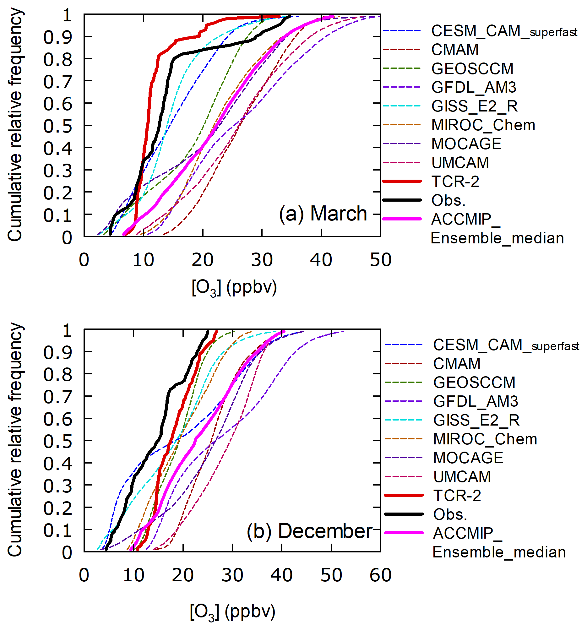
Figure 12 Cumulative relative frequency distributions of O₃ mixing ratios from observations (black), TCR-2 (red), and members and ensemble median of ACCMIP for domain 3 (0–15^∘ N and 150–165^∘ E) in (a) March and (b) December.

The average relative diurnal variations normalized to the maximum mixing ratios during these 2 months (Fig. 13, x axis is UTC+11 h, adjusted to local time for the selected region) showed a pattern of daytime decreases, suggesting photochemical destruction. However, the observed decrease was stronger (15 %) and earlier than those simulated in the TCR-2 and ACCMIP runs, in which the HO_x cycle was primarily responsible for photochemical destruction. This feature may indicate O₃ loss via a different process, e.g., halogen chemistry, which is not included in any of the model simulations considered in this study.

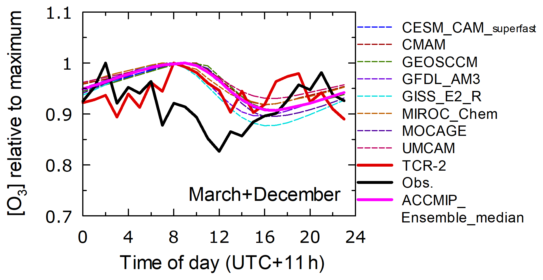
Figure 13 Diurnal variation patterns relative to maximum mixing ratios from observations (black), TCR-2 (red), and members and ensemble median of ACCMIP for domain 3 (0–15^∘ N and 150–165^∘ E). Data from March and December are merged.

To obtain further insights into the regions in which this additional loss could be important, the differences between the O₃ levels predicted by TCR-2 and the observed levels were calculated and the correlations with the residence times (in the daytime) of back trajectories in 15^∘ × 15^∘ grid regions around domain 3 were examined. Use of the residence time during the day can be justified because the destruction probably occurred in the daytime (Fig. 13). Figure S2 shows the results for 17 regions, covering 120–195^∘ E and 15^∘ S to 45^∘ N. We found that the residence time in the grid region 165–180^∘ E and 15–30^∘ N, located northeast of domain 3, had the largest positive correlation coefficient (Fig. 14). This suggests that this region is a possible hotspot for additional loss. It is worth noting that data from all five cruises contributed to the positive correlation, which suggests that the relationship is reproducible. The slope of the regression line was 0.25 ppbv h⁻¹. This corresponds to the possible loss rate in the grid that best explains the discrepancy between observations and TCR-2 predictions. If the rate is attributed to dry deposition on the sea surface, a deposition velocity as high as 0.33 cm s⁻¹ is required, assuming a boundary layer height of 1000 m and an average O₃ mixing ratio of 17.4 ppbv. This high velocity is not supported by previous studies (e.g., Ganzeveld et al., 2009; Hardacre et al., 2015). Such a loss rate can be more easily explained by bromine and/or iodine chemistry in the atmosphere (e.g., Saiz-Lopez et al., 2012, 2014). We observed elevated iodine monoxide (IO) radical concentrations with a MAX-DOAS instrument aboard R/V Mirai during the cruises included in the analysis in Fig. 14. Further analysis will be reported in a future publication.

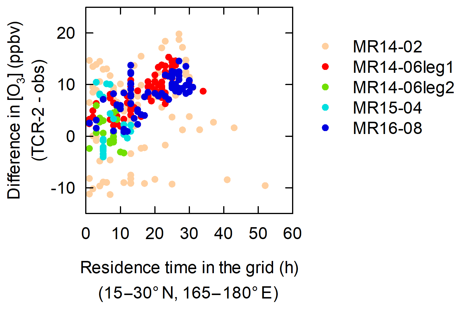
Figure 14 High biases in TCR-2 with respect to observations in domain 2 (10^∘ S to 25^∘ N, 125–165^∘ E) show positive correlations with daytime residence times in grid 15–30^∘ N and 165–180^∘ E.

Substantially reduced O₃ levels (< 10 ppbv) have been reported in the marine boundary layer over the equatorial Pacific. Johnson et al. (1990) found near-zero (3 ppbv or less) O₃ mixing ratios in the central equatorial Pacific during April and May. Kley et al. (1996) observed similar events in March 1993, with mixing ratios occasionally reaching 3–5 ppbv, from O₃ soundings in a region between the Solomon Islands (9.4^∘ S, 160.1^∘ E) and Christmas Island (2^∘ N, 157.5^∘ W). Takashima et al. (2008) reported substantially reduced O₃ events throughout the year on Christmas Island. Rex et al. (2014) used a combination of O₃ sounding data from the TransBrom cruise of R/V Sonne in October 2009, atmospheric chemistry models, and satellite observations to identify a region with strong O₃ depletion in the marine boundary layer at 0–10^∘ N along the north–south cruise track (at around 150^∘ E). This is in good agreement with our observations. Hu et al. (2010) reported that average O₃ mixing ratios at Kwajalein Island (8.72^∘ N, 167.73^∘ E), Republic of the Marshall Islands, located near our hotspot grid, during July, August, and September 1999, were lower than 10 ppbv throughout 24 h, with an afternoon decrease of about 1 ppbv. Gómez Martín et al. (2016) reported year-round continuous observations of surface O₃ at San Cristóbal (0.90^∘ S, 89.61^∘ W) and at Puerto Villamil, Isabela Island (0.96^∘ S, 90.97^∘ W), in the Galápagos Islands in the equatorial eastern Pacific. Daily averages as low as 5–6 ppbv were observed during the period February to May. During the Malaspina circumnavigation in 2010, O₃ mixing ratios as low as 3.4 ppbv were detected around the central Pacific equatorial region (Prados-Roman et al., 2015). During PEM-West A in October 1991, Singh et al. (1996) reported O₃ levels as low as 8–9 ppbv from aircraft measurements at altitudes of 0.3–0.5 km in the region 0–20^∘ N in the western and central Pacific. It is worth noting that the O₃ levels over the Atlantic were typically higher, e.g., 30–35 ppbv (Read et al., 2008), even when halogen-mediated destruction was considered. In these studies, detailed statistical comparisons of the observed O₃ levels with chemistry–climate model simulations or reanalysis data as focused here have not been achieved. Conducting continuous observations of O₃ during a large number of cruise legs was useful for obtaining a large data set for performing detailed statistical analysis.

The influence of halogen (bromine and/or iodine) chemistry on O₃ levels has been studied using model simulations at assumed (e.g., Davis et al., 1996; Hu et al., 2010) and observed levels of halogen compounds (Mahajan et al., 2012; Dix et al., 2013; Großmann et al., 2013; Prados-Roman et al., 2015; Koenig et al., 2017) over the Pacific. For example, for bromine chemistry, Hu et al. (2010) estimated a photochemical loss rate of up to 0.12 ppbv h⁻¹. A loss of about 0.4 ppbv d⁻¹ can be attributed to halogen chemistry in the marine boundary layer south of Hawaii (Dix et al., 2013). From CAM-chem-based global model simulations, Saiz-Lopez et al. (2012) estimated an annually integrated rate of surface O₃ loss through halogen chemistry as ∼0.15 ppbv h⁻¹ in the daytime, over the region 20^∘ S to 20^∘ N. On the basis of GEOS-Chem, Sherwen et al. (2016) suggested that halogen chemistry would reduce surface O₃ levels by ∼3–5 ppbv over our domain 3. These loss rates caused by halogen chemistry are in fair agreement with the required additional loss rate, i.e., ∼0.25 ppbv h⁻¹, estimated in this study.

Our observational O₃ data set with a large geographical coverage will be useful for evaluating up-to-date model simulations with inclusion of halogen chemistry. Analysis at midlatitude regions over the Pacific are also of interest because the importance of halogen chemistry in this region has been indicated (e.g., Nagao et al., 1999; Galbally et al., 2000; Watanabe et al., 2005).

4 Summary and outlook

We compiled a large data set of shipborne in situ observations of O₃ and CO levels with a 1 h resolution, which were recorded on R/V Mirai over the Arctic, Bering, Pacific, Indian, and Southern oceans from 67^∘ S to 75^∘ N, during the period 2012 to 2017. We used the data set to evaluate tropospheric chemistry reanalysis data from TCR-2 and ACCMIP model simulations. TCR-2 captured the basic features of the observations, including the latitudinal gradient and air mass exchange, and therefore enabled interpretation of observations regarding transport and pollution sources. Correlations with observations were sufficient (R² up to 0.62 for hourly data and 0.67 for daily data). This suggests an excellent performance by TCR-2 in representing the temporal and geographical distributions of surface O₃. For over 23 long-range transport events with CO and/or O₃ buildup, variations in the ΔO₃∕ΔCO ratios were well reproduced by TCR-2. This suggests that the nature of photochemical evolution during transport of pollution plumes was also well captured. However, two major discrepancies were identified: in the Arctic (> 70^∘ N) in September, TCR-2 and the ensemble median of model runs of ACCMIP tended to underestimate O₃ levels. From analysis of O₃ sonde measurements, we concluded that the gap was related to processes relevant to the boundary layer: downward mixing from the free troposphere, with a higher O₃ abundance, might have been too weak in the models. For TCR-2, dry deposition on the Arctic Ocean surface might have been too fast. Conversely, in the western Pacific equatorial region, TCR-2 and ACCMIP simulations significantly overestimated the observed O₃ levels, which were often less than 10 ppbv. The minimum in the observed diurnal pattern occurred earlier than those in the models. The gap of mixing ratios correlated with the residence time of trajectories over a particular grid, i.e., 15–30^∘ N, 165–180^∘ E. These analyses indicate the importance of halogen chemistry, which is not accounted for in the models, and the region in which it is active. The data set from our observations (which will continue) is open and complements the TOAR data collection and will be useful for critically evaluating global-scale atmospheric chemistry model simulations, including those from CCMI, AerChemMIP (Collins et al., 2017), and future intermodel comparisons.