the Creative Commons Attribution 4.0 License.
the Creative Commons Attribution 4.0 License.
 | 18 Jan 2019
Biogenic emissions and land–atmosphere interactions as drivers of the daytime evolution of secondary organic aerosol in the southeastern US
Juhi Nagori
Ruud H. H. Janssen
Juliane L. Fry
Maarten Krol
Jose L. Jimenez
Weiwei Hu
Jordi Vilà-Guerau de Arellano
The interactions between biogenic volatile organic compounds (BVOCs), like isoprene and monoterpenes, and anthropogenic emissions of nitrogen and sulfur oxides lead to high concentrations of secondary organic aerosol (SOA) in the southeastern United States. To improve our understanding of SOA formation, we study the diurnal evolution of SOA in a land–atmosphere coupling context based on comprehensive surface and upper air observations from a characteristic day during the 2013 Southern Oxidant and Aerosol Study (SOAS) campaign. We use a mixed layer model (MXLCH-SOA) that is updated with new chemical pathways and an interactive land surface scheme that describes both biogeochemical and biogeophysical couplings between the land surface and the atmospheric boundary layer (ABL) to gain insight into the drivers of the daytime evolution of biogenic SOA.
MXLCH-SOA reproduces observed BVOC and surface heat fluxes, gas-phase chemistry, and ABL dynamics well, with the exception of isoprene and monoterpene mixing ratios measured close to the land surface. This is likely due to the fact that these species do not have uniform profiles throughout the atmospheric surface layer due to their fast reaction with OH and incomplete mixing near the surface. The flat daytime evolution of the SOA concentration is caused by the dampening of the increase due to locally formed SOA by entrainment of SOA-depleted air from the residual layer. SOA formation from isoprene through the intermediate species isoprene epoxydiols (IEPOXs) and isoprene hydroxyhydroperoxides (ISOPOOHs) is in good agreement with the observations, with a mean isoprene SOA yield of 1.8 %.
However, SOA from monoterpenes, oxidised by OH and O3, dominates the locally produced SOA (69 %), with a mean monoterpene SOA yield of 10.7 %. Isoprene SOA is produced primarily through OH oxidation via ISOPOOH and IEPOX (31 %). Entrainment of aged SOA from the residual layer likely contributes to the observed more oxidised oxygenated organic aerosol (MO-OOA) factor.
A sensitivity analysis of the coupled land surface–boundary layer–SOA formation system to changing temperatures reveals that SOA concentrations are buffered under increasing temperatures: a rise in BVOC emissions is offset by decreases in OH concentrations and the efficiency with which SVOCs partition into the aerosol phase.
- Article
(4947 KB) - Full-text XML
- BibTeX
- EndNote


Secondary organic aerosol (SOA) produced from the oxidation of volatile organic compounds (VOCs) forms an important contribution to aerosol loading (Jimenez et al., 2009; Zhang et al., 2007). They can affect regional climate (Goldstein et al., 2009) and pose health risks to humans (Mauderly and Chow, 2008). A large fraction of SOA is formed by biogenic volatile organic compounds (BVOCs), which are emitted in large quantities from forested areas, especially during summer (Goldstein et al., 2009; Guenther et al., 1995). Isoprene and the monoterpenes α-pinene, β-pinene, and limonene are the most abundant of these BVOCs in the southeastern US (Liao et al., 2007). Consequently, SOA mass in this region has a high biogenic contribution (Ahmadov et al., 2012; Kim et al., 2015).
Anthropogenic emissions can alter the oxidation pathways of BVOCs and thereby the formation of SOA from biogenic precursors (Spracklen et al., 2011). Recently, the contribution of isoprene to SOA in the southeastern US has been studied extensively, with a focus on aqueous-phase reactive uptake mechanisms that are modulated by anthropogenic emissions of sulfur dioxide (SO2) (Budisulistiorini et al., 2015; Hu et al., 2016). In addition, isoprene SOA can also be produced through the condensation of low-volatility organic compounds (LVOCs) (Krechmer et al., 2015). Both mechanisms are prevalent under low nitrogen monoxide (NO) conditions, which are important at the SOAS site, under which the initial oxidation of isoprene by the hydroxyl radical (OH) leads to the formation of hydroxyhydroperoxides (ISOPOOHs) (Paulot et al., 2009), whose oxidation product (ISOP(OOH)2) can condense to form ISOPOOH SOA. The major channel of ISOPOOH oxidation, however, forms isoprene epoxydiols (IEPOXs), which produce IEPOX SOA upon reactive uptake on acidic surfaces (Gaston et al., 2014; Hu et al., 2016; Krechmer et al., 2015). IEPOX SOA formation contributed approximately 15 %–30 % to total observed aerosol mass during the SOAS campaign, while ISOPOOH SOA contributed approximately 2.2 % (Krechmer et al., 2015; Lopez-Hilfiker et al., 2016b).
Monoterpene SOA (MT SOA) formation has been shown to be important in the southeastern US (Kim et al., 2015; Xu et al., 2018; Zhang et al., 2018) and depends on anthropogenic nitrogen oxide (NOx) emissions, which influence daytime oxidation pathways and enhance nitrate-radical-initiated (NO3) SOA formation during night-time (Ayres et al., 2015; Xu et al., 2015).
Sesquiterpene oxidation and the resulting SOA are not included due to its small contribution to SOA during SOAS (3 % compared to ∼45 % for monoterpenes and ∼18 % for isoprene) (Hu et al., 2015; Marais et al., 2016; Zhang et al., 2018). Sesquiterpenes are very reactive and those contributions could be underestimated. However, without further information that would suggest a larger importance in the SE US, we did not include sesquiterpenes in the current study.
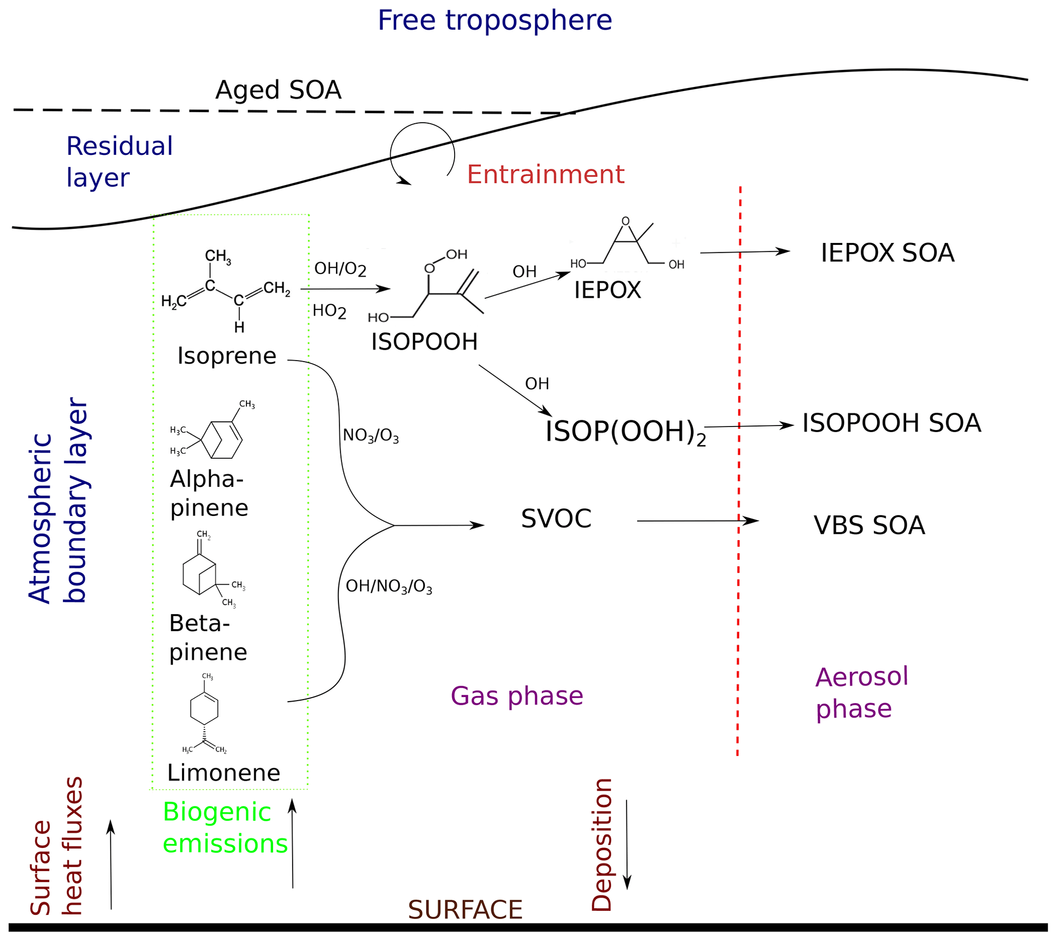
Figure 1Formation pathways of secondary organic aerosol (SOA) and interactions included in this study. The atmospheric layers in consideration are shown in blue, and dynamic and surface processes are shown in maroon. The chemical species are in black, the arrows show their movement, and the stages the species go through are shown in purple. Biogenic emissions of gas-phase precursors at the land surface are followed by oxidation by OH, O3, and NO3 to form semi-volatile organic compounds (SVOCs), which either partition between the gas phase and aerosol phase, condense to the aerosol phase, or form aerosol through reactive uptake onto existing acidic aerosol. ISOPOOH and IEPOX are the isoprene oxidation products isoprene hydroxy hydroperoxides (ISOPOOHs) and isoprene epoxydiols (IEPOXs), respectively. VBS SOA stands for SOA formed through gas–particle partitioning in the volatility basis set. SOA formation takes place in the atmospheric boundary layer (ABL), which grows in time due to surface fluxes. Entrainment of air from the residual layer brings in aged SOA from previous days and long-range transport.
Since SOA concentrations in the southeastern US are driven by both natural and anthropogenic factors, understanding future changes in SOA concentrations requires an understanding of these different factors and their interactions. Previous modelling studies have focused on the effects of future lower anthropogenic emissions of NOx and sulfur oxides (SOx) on the formation of isoprene-derived SOA (Marais et al., 2016; Pye et al., 2013). These studies found that reductions of anthropogenic emissions of NOx and SOx lead to a net reduction of SOA formation from isoprene.
Here, we study the formation of SOA from biogenic emissions (specifically from daytime sources) and the SOA diurnal evolution in the context of land–atmosphere coupling, including both biogeochemical interactions (VOC emissions) and biogeophysical interactions (sensible and latent heat fluxes) between the land surface and the atmosphere, in a case study for the SOAS campaign. The diurnal SOA evolution is driven by atmospheric boundary layer (ABL) dynamics and the interaction between the ABL and the free troposphere (FT), as well as by emissions, chemical transformations, and subsequent partitioning into the aerosol phase (Janssen et al., 2012, 2013). The ABL dynamics are often a challenge to represent in global and regional chemistry models; hence, in order to encompass the many aforementioned factors affecting the diurnal SOA evolution, an integrated approach is required to accurately represent the diurnal evolution of SOA and BVOC concentrations.
As sources of SOA, we consider isoprene SOA formation through aqueous-phase uptake of IEPOX (Hu et al., 2015; Marais et al., 2016) and through condensation of ISOP(OOH)2 (Krechmer et al., 2015), and speciated monoterpene SOA formation from α-pinene, β-pinene, and limonene. We account for the anthropogenic influence on biogenic SOA formation by including the influence of NOx concentrations on peroxy radical chemistry, in addition to the NOx-induced changing ratios of oxidant concentrations (OH, NO3, ozone (O3)). We do not include night-time SOA formation.
Our aim is twofold: (1) to improve our understanding of SOA formation in the southeastern US from established and recently elucidated pathways and (2) to understand SOA diurnal evolution in a land–atmosphere coupling context. We build on the case study by Su et al. (2016) that was able to accurately reproduce the dynamics and gas-phase photooxidation of isoprene during the SOAS campaign and then do the following.
-
We couple the dynamics and chemistry of the boundary layer–chemistry model to the land surface and vegetation factors by including interactive formulations for surface BVOC and heat fluxes.
-
We update the SOA formation module by including speciated monoterpenes and isoprene SOA formation through reactive uptake and condensation to accurately represent the diurnal SOA evolution, as constrained by tower and aircraft observations. Figure 1 shows a schematic of the chemistry mechanism.
-
We study the contribution of different aerosol factors in the southeastern US and attempt to identify the source contributions to more oxidised oxygenated organic aerosol (MO-OOA).
-
We analyse the SOA budget and quantify the contribution of different processes and precursors to the SOA diurnal evolution.
-
Finally, we carry out a sensitivity of the integrated land surface–boundary layer–SOA formation system to concentrations of SOA in the residual layer (RL) and to temperature changes.
To constrain and evaluate our model, we use data collected during the Southeastern Oxidant and Aerosol Study (SOAS), held over the period of 1 June to 15 July 2013 (Hidy et al., 2014), and the Southeast Nexus (SENEX) campaign, held in the same time period (Warneke et al., 2016). Both campaigns were part of the Southeast Atmosphere Studies (SAS), which coordinated comprehensive measurements of trace gas and aerosol compositions, aerosol physics and chemistry, and meteorological dynamics across the southeastern US (Carlton et al., 2018). All the measurements (and model results) are shown in Central Standard Time (CST).
The case study represents the SOAS main sites near Brent (32∘54′12 N, 87∘15′0 W) and Marion (32∘41′40 N, 87∘14′55 W), Alabama; these are the SOAS ground and flux (above-canopy) measurement sites, respectively. A pre-existing Southeastern Research and Characterization (SEARCH) network site served as the main ground site with gas chromatography–mass spectrometry (GC-MS) (including speciated monoterpene mixing ratios) (Su et al., 2016) and aerosol mass spectrometry (AMS) measurements (Hu et al., 2015). The National Center for Atmospheric Research C-130 flights collected observations of trace gases, isoprene, monoterpenes, photolysis, methyl vinyl ketone (MVK), and methacrolein (MACR) (Warneke et al., 2016). At the Alabama Aquatic Biodiversity Center (AABC) flux tower (24 km from the Brent ground site and tower) eddy covariance measurements above canopy for surface latent and sensible heat, BVOC fluxes, and shear velocity (u*) measurements were carried out. We use data from both sites to represent a more regional footprint. Flights with the Whole Air Sample Profiler (WASP) and high-resolution proton transfer reaction time-of-flight mass spectrometer (PTR-ToF-MS) measured trace gas concentrations, meteorological data, and isoprene and monoterpene mixing ratios above the AABC tower (Su et al., 2016), though speciated monoterpenes mixing ratios are only obtained through GC-MS at the SEARCH site. Data are also used from the NOAA P-3 flights during the Southeast Nexus (SENEX) campaign, which included vertical profile data near the SOAS site (Warneke et al., 2016). To reduce uncertainties from day-to-day variations and gain representativity, we average the meteorological data, isoprene and monoterpene emissions and mixing ratios, and trace gas mixing ratio data for 5, 6, 8, and 10–13 June following Su et al. (2016). The speciated monoterpene data from the GC-MS measurements are averaged from 5–13 June. WASP research flights were not flown on 7 and 9 June (Su et al., 2016), whereas GC-MS had continuous data.
The total organic aerosol (OA) concentrations measured at the SOAS site by the AMS (Canagaratna et al., 2007; DeCarlo et al., 2006) have previously been apportioned by positive matrix factorisation (PMF) to determine the contribution of individual SOA factors (Ulbrich et al., 2009) (see discussion below). The main SOA factors observed at the SEARCH site were isoprene-epoxydiol-derived SOA (IEPOX SOA), isoprene hydroxyhydroperoxide SOA (ISOPOOH SOA), more oxidised oxygenated OA (MO-OOA), low oxidised oxygenated OA (LO-OOA), and biomass burning OA (BBOA) (Hu et al., 2015; Xu et al., 2015); the total observed SOA is the sum of all these factors. For this study, the aerosol data are averaged for 6, 8, and 10–13 June, since data are not available for 5 June and are incomplete for 7 and 9 June (Hu et al., 2016, 2015; Krechmer et al., 2015; Xu et al., 2015).
We use a mixed layer model for the dynamics of the convective boundary layer with a chemistry and SOA formation module (MXLCH-SOA) to analyse a representative (sub-diurnal) case study for the southeastern US. The model version that we use is described in Su et al. (2016) and Janssen et al. (2013), and a derivation of its basic equations is given in Vilà-Guerau de Arellano et al. (2015). The dynamics and boundary conditions can be seen in Table A1. In this section, we summarise the main characteristics of the model and in the following subsections we describe the specific adaptations that have been made for this study, which include new chemical pathways (Sect. 3.1), SOA formation mechanisms (Sect. 3.2), interactive BVOC emissions (Sect. 3.3), and a coupled land surface model (Sect. 3.4).
MXLCH-SOA approximates ABL mixing under convective conditions (Lilly, 1968; Tennekes, 1973) by assuming vigorous mixing throughout the daytime ABL, resulting in constant mixing ratios with height. The ABL height growth due to entrainment is driven by sensible and latent heat flux (Tennekes, 1973). We consider the atmospheric boundary layer interface with the free troposphere to be an infinitesimal inversion layer with entrainment-driven exchange of scalars and variables between these layers (Tennekes and Driedonks, 1981), i.e. a zero-order closure model. Large-scale meteorology is prescribed based on Su et al. (2016), species segregation is neglected (Ouwersloot et al., 2011), and we do not account for horizontal advection via long-range transport.
The chemical reaction scheme, which consists of the essential gas-phase reactions of the O3–NOx–VOC–HOx system (see Table ), is based on Su et al. (2016) and Janssen et al. (2013). The standard SOA formation scheme in MXLCH-SOA is based on the volatility basis set (VBS) approach (Donahue et al., 2006).
3.1 New chemical pathways
We add gas-phase reactions that lead to IEPOX SOA and ISOPOOH SOA formation (Reactions RA19, RA30–RA34) from Hu et al. (2016). To better represent IEPOX SOA formation, we included a module for reactive uptake (Sect. 3.2.2) (Gaston et al., 2014; Hu et al., 2016). The reactions of speciated monoterpenes (α-pinene, β-pinene, and limonene) with the three oxidants (OH, O3, and NO3) are also added (Reactions RA38–RA46), as are reactions of isoprene with O3 and NO3 (Reactions RA36–RA37) (Atkinson and Arey, 2003; Crounse et al., 2011; Orlando and Tyndall, 2012; Pye et al., 2010; Wennberg et al., 2018). The IRO2+HO2 and IRO2+NO rate constants are updated per Crounse et al. (2011). We use the speciated monoterpenes α-pinene, β-pinene, and limonene (the most abundant monoterpenes in the southeastern US; Geron et al., 2000) instead of the bulk monoterpene term which is used in Janssen et al. (2012). With these new pathways we can track the actual variability in SOA formation due to different BVOC precursor–oxidant combinations. The contributions to SOA can be quite different depending on the combination; for instance, limonene + OH or O3 in high NOx has a yield of 0.62 at 10 µg m−3, whereas β-pinene and NO3 have a yield of 0.26 (Geron et al., 2000; Pye et al., 2010). We also add the BVOC+NO3 oxidation reactions to the VBS module as NO3-initiated oxidation has been shown to contribute substantially to SOA loading (Ayres et al., 2015; Fisher et al., 2016; Pratt et al., 2012). Nitrate-radical-initiated oxidation is dominant during night-time (as the lifetime of NO3 is very short during daytime), and organonitrate formation peaks at night-time as well (Xu et al., 2015). This is because monoterpene emissions, unlike isoprene emissions, persist after sundown (Ayres et al., 2015; Horowitz et al., 2007).
3.2 Secondary organic aerosol formation
In the MXLCH-SOA model we represent the isoprene + OH factors explicitly using the full mechanism for the formation of IEPOX SOA and ISOPOOH SOA (Hu et al., 2016; Krechmer et al., 2015). We then aggregate the other SOA formation via O3 and NO3 with isoprene and all oxidants with monoterpenes via volatility basis set (VBS) partitioning for comparison with MO-OOA and LO-OOA (Donahue et al., 2006). However, it is uncertain how much of the aged MO-OOA is locally formed versus advected in via long-range transport, and we apply a simulation with no entrainment in an attempt to separate these effects. This is explored in Sect. 7, in which different residual layer SOA concentrations are applied to explore their effect on the diurnal evolution of SOA in the ABL. The IEPOX SOA is formed through reactive uptake and a mechanism to calculate the heterogeneous reaction rate for this formation is included (Gaston et al., 2014; Hu et al., 2016). Lastly, ISOPOOH SOA formation (upon condensation) is included using reaction rates from Krechmer et al. (2015). BBOA is not accounted for in the model; however, as G–P partitioning depends on the total aerosol mass in the system, it is included in the initialisation of background SOA. We do not consider isoprene SOA formed through the methacryloyl peroxynitrate (MPAN) pathway (Kjaergaard et al., 2012), since this pathway had a negligible contribution to SOA formation during the SOAS campaign (Nguyen et al., 2015a), as it is favoured under low temperatures and high NO2 conditions.
3.2.1 Gas–particle partitioning
SOA formation through gas–particle (G–P) partitioning in the MXLCH-SOA model follows the volatility basis set (VBS) approach (Donahue et al., 2006), with semi-volatile products of VOC oxidation lumped into four logarithmically spaced bins of effective saturation concentration.
The SVOC yields for isoprene, α-pinene, β-pinene, and limonene are obtained from Pye et al. (2010) and are summarised in Table A3. These yields depend on NOx concentrations, with the high and low NOx yields interpolated based on the branching reaction of RO2 from isoprene and monoterpene through NO and HO2 channels. We do not consider G–P partitioning of the products of the isoprene + OH reaction since this reaction is explicitly accounted for via ISOPOOH SOA and IEPOX SOA formation through condensation and reactive uptake, which are assumed to form low-volatility aerosol products (Hu et al., 2016; Krechmer et al., 2015; Lopez-Hilfiker et al., 2016a). The β-pinene reaction rates are used here as a proxy for monoterpene branching, and the reaction with NO and HO2 has rates of cm3 molec−1 s−1 and cm3 molec−1 s−1 (Saunders et al., 2003), respectively, while the reaction rates for isoprene are the same, as shown in Table . For the enthalpy of vaporisation we use the recommended value of 42 kJ mol−1 from Pye et al. (2010).
We prescribe an early morning SOA concentration (OABG) (Janssen et al., 2012), which has the assumed initial value of 3.2 µg −3 in the ABL based on total SOA observations at SOAS (see Fig. 7) and 1.5 µg m−3 above the ABL based on vertical profiles (Fig. C4). The effective saturation concentrations are based on Pye et al. (2010), which are more relevant to the southeastern US (Table A3). A deposition velocity of 0.024 m s−1 was set for the SVOCs, as per Karl et al. (2010). The dry deposition of SOA is not considered as it is small at approximately 0.002 m s−1 (Farmer et al., 2013).
3.2.2 Reactive uptake and condensation
IEPOX SOA and ISOPOOH SOA formation results from the isoprene + OH reaction (RA9). The initially formed isoprene peroxy radical IRO2 reacts with OH to give isoprene hydroxyhydroperoxides (ISOPOOHs). ISOPOOH reacts with OH and forms either isoprene epoxide (IEPOX) (Paulot et al., 2009) or ISOP(OOH)2 (Liu et al., 2016). ISOPOOH SOA is formed due to condensation of ISOP(OOH)2 to the aerosol phase, with a yield of 4 % (from ISOPOOH + OH). A deposition velocity of 0.03 m s−1 is applied for ISOPOOH and IEPOX, as per Nguyen et al. (2015b).
A heterogeneous reaction rate for IEPOX SOA formation is calculated using a modified resistor model from Gaston et al. (2014) and using inputs from Hu et al. (2016) to represent SOAS conditions. A γIEPOX factor is used to determine the lifetime of IEPOX against aerosol uptake. This factor depends on pH, temperature, particle size, nucleophile (sulfates and nitrates) and hydrogen sulfate ion () concentration, the mass accommodation coefficient, and the radius of the inorganic core, which was estimated from a volume ratio between organics and inorganics from the AMS data (Gaston et al., 2014; Hu et al., 2016). The values for these parameters were constrained by the ambient aerosol measurements as described in Hu et al. (2016). The IEPOX SOA was a considerable fraction of the organic aerosol mass measured during SOAS, approximately 17 % (Hu et al., 2015), while ISOPOOH SOA explains a small fraction of aerosol formed through low-NO isoprene oxidation (Krechmer et al., 2015); hence, they are included to represent the aerosol composition for the SOAS campaign.
3.3 Biogenic volatile organic compound emissions
We implement the Model of Emissions of Gases and Aerosols from Nature (MEGAN) (Guenther et al., 2006) to calculate monoterpene and isoprene emission fluxes, driven by light intensity and the temperature of the overlying atmosphere. In this model, emissions of isoprene and monoterpenes are parameterised depending on base emissions, the production and loss of BVOC within canopy, and the emission activity factors. The base emission rates depend on the plant functional type, which are taken as a broadleaf forest at the SOAS site (Guenther et al., 2006). The isoprene fluxes are light dependent so we use the parameterised canopy environment emission activity (PCEEA), and we use air temperature instead of skin temperature in our formalism, as the PCEEA already accounts for the canopy temperature being higher than air temperature (Alex Guenther, personal communication, 2017). The daily average photosynthetic photon flux density (PPFD) was calculated between 400 and 500 µmol m−2 s−1 for this site (Alex Guenther, personal communication, 2017). We use a conversion factor of 4.766 to convert the photosynthetically active radiation (PAR) value from W m−2 to PPFD above canopy in µmol m−2 s−1, per the Goddard Earth Observing System chemistry (GEOS-chem) model. We calculate the monoterpene flux depending on the canopy emission activity factor and the soil moisture emission activity factor and use skin temperature instead of air temperature (Guenther et al., 1995). Table A5 summarises the MEGAN parameters applied here.
To derive speciated monoterpene emissions, factors of 45 % : 45 % : 10 % are applied to allocate the emissions to α-pinene, β-pinene, and limonene, respectively, based on their average relative abundances observed during the SOAS campaign as per Fig. S1 in Ayres et al. (2015).
3.4 Coupled land surface model
The land surface and the boundary layer form a tightly coupled system, in which fluxes respond to changes in forcings on the whole system (Betts, 2004; Van Heerwaarden et al., 2009). To properly understand the response of SOA formation to changing temperatures (see Sect. 8), it is therefore important to have a fully coupled land surface–boundary layer model. This allows us to study the effects on SOA evolution of a forcing which affects the coupled land–atmosphere. For that purpose, a land surface model (Van Heerwaarden et al., 2009) is coupled to MXLCH-SOA to obtain a fully coupled land surface–boundary layer model that enables the interactive calculation of surface heat fluxes based on the Penman–Monteith equations for evapotranspiration (Monteith, 1965). With this inclusion, MXLCH-SOA can be used to simultaneously and interactively calculate the exchange of energy (sensible heat flux) and water (latent heat flux) between the land surface and the ABL. These heat fluxes, in turn, drive the diurnal dynamics of the ABL. Additionally, the coupled land surface model also provides input for calculating BVOC emissions interactively (Sect. 3.3).
In this way, an online coupled land surface–ABL–SOA formation model is obtained, in which the exchanges of energy and VOCs between the land surface and the ABL at the diurnal timescale are internal variables of the coupled system. This means that only forcings (drivers external to the system at the appropriate timescales) are prescribed to the model. Note that dry deposition is not yet calculated interactively; we instead utilise deposition velocities from other literature. We evaluate the interactively calculated surface moisture and heat fluxes with the eddy covariance measurements taken at the AABC tower.
Table A4 shows the land surface characteristics used to calculate the dynamic fluxes interactively, for which typical values for broadleaf trees are used. We model above canopy and include a wind module in which the initial U wind and V wind are set at 1 m s−1. These wind module values are used so as to have a more realistic value of the aerodynamic resistance, ra, which is otherwise very large in the first time step due to a very small convective velocity scale, w*. The ra is inversely proportional to w* in the model.
We use the MXLCH-SOA model to perform a set of numerical experiments to improve our understanding of SOA formation during SOAS in a land–atmosphere coupling context. First, we set up a base case by expanding the case study of Su et al. (2016) guided by the observations of heat and VOC fluxes, ABL dynamics, and VOC and SOA concentrations. We then evaluate the contributions of the different dynamical and chemical processes to the diurnal evolution of the SOA concentration and dissect the SOA budget to show the contributions of the various precursors and chemical pathways to SOA formation.
The dynamical initial and boundary conditions for the base case are shown in Table A1 and are based on Su et al. (2016). We apply a lapse rate of 0.002 K m−1 below 1150 m and 0.005 K m−1 above 1150 m to better constrain the boundary layer height (See Fig. 3). The lapse rate mimics upper air conditions and counteracts the development of the ABL, and we adjust this value so that the observed evolution of the boundary layer was satisfactorily reproduced by the model (See Fig. 3). The initial conditions for the chemical species are based on observations from the SEARCH and AABC sites and Su et al. (2016) (see Table A6). Early morning NOx chemistry and subsequent SOA formation is constrained by the initialisation of NO and NO2 mixing ratios at 06:00 CST based on observed mixing ratios (see Fig. C1). The initial concentrations of SOA in the boundary layer are based on AMS observations taken at the SEARCH site (Hu et al., 2015). Since the model is initialised at sunrise, it does not explicitly account for night-time SOA formation, but the effect of NO3-initiated night-time SOA formation is included in the value of the prescribed bulk SOA concentration.
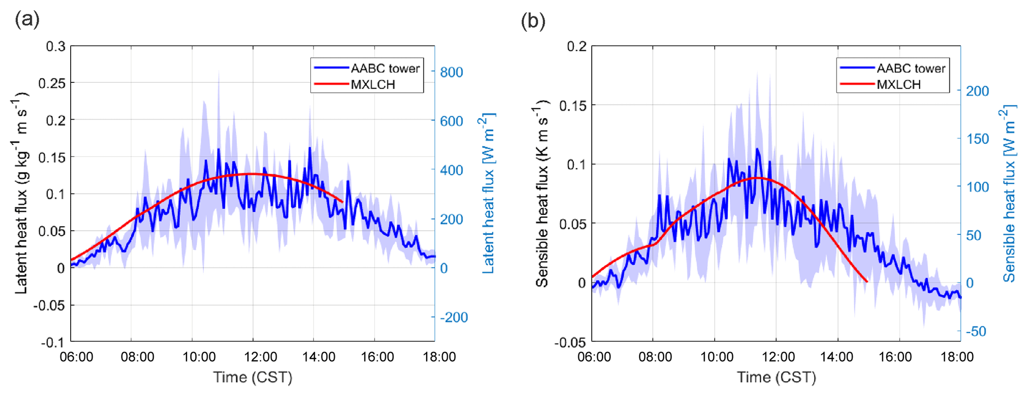
Figure 2(a) Sensible and (b) latent heat flux measured (blue) and modelled (red) at the Alabama Aquatic Biodiversity Center (AABC) eddy covariance tower. The blue shaded area represents the data variability over 5, 6, 8, and 10–13 June 2013, while the solid blue shows the average over these days.
After establishing the base case, we carry out a series of numerical experiments to assess the impact of SOA concentrations above the ABL on the diurnal SOA evolution to stress the importance of information on early morning residual layer concentrations. We use concentrations measured above the ABL, as we have a few measurements of SOA concentration at 11:00 CST from SENEX flights (Warneke et al., 2016). In addition to the base case in which SOA in the RL was initiated at 1.5 µg m−3, we also run simulations in which we initiated it at 1 and 1.8 µg m−3, respectively, which encompasses the range of observed SOA concentrations above the ABL. Further, we included a scenario in which SOA concentrations in the ABL and RL were initialised with uniform values. The latter scenario is then used to estimate the contribution of long-range transport versus local formation of MO-OOA.
Finally, we explore the effect of a changing climate on the near-surface SOA concentration. Our main interest is improving our understanding of the net effect on SOA concentrations of several interacting processes that can either reinforce or compensate for each other. The increase in average air temperature under a warmer climate has several effects on the coupled system that may affect SOA concentrations: (1) VOC emissions increase, (2) the partitioning efficiency of SVOCs into the aerosol phase decreases, and (3) the vapour pressure deficit (VPD) decreases, which modulates the heat fluxes and consequently the boundary layer height (Van Heerwaarden et al., 2009). We simulate a warming climate of 1 and 2 K. For this purpose, the early morning values of mixed layer temperature, surface temperature, and soil temperature in both layers are all increased (and decreased) by 1 and 2 K. In order to stay consistent with climate warming predictions, the initial relative humidity is kept constant, which is done by calculating the values of the specific moisture at each temperature increment using the Clausius–Clapeyron relation (Van Heerwaarden et al., 2009). In this way the sensible heat flux forcing is more consistent with future climate warming. As previous literature (Goldstein et al., 2009; Hansen et al., 1999, 2001) has observed the southeastern US to have undergone a cooling trend compared to the rest of the US in the summer months, we add two more runs with a cooling of 1 and 2 K, respectively.
5.1 Surface heat and BVOC fluxes
We are able to successfully represent the dynamics, surface conditions, and gas-phase chemistry and hence have a good balance of the three in this model. The correspondence of the model to those observations is comparable to Su et al. (2016).
Figure 2 shows that the interactively calculated sensible and latent heat fluxes match well with the observations. The modelled sensible heat flux peaks before noon (at around 100 W m−2) and is underestimated compared to the observations at the end of the afternoon. However, measurements are largely in the range of observations and eddy covariance measurements have an uncertainty range of approximately 15 %–20 %, as measurements mostly underestimate the fluxes (possibly due to unresolved eddies) (Field et al., 1992; Weaver, 1990). The modelled latent heat flux matches the observations and peaks at noon (just below 0.14 g kg−1 m s−1 or 400 W m−2). The Bowen ratio (the ratio of the sensible heat to the latent heat) is consistent with being above a moist surface, as the latent heat flux is larger than the sensible heat flux.

Figure 3Boundary layer height measured (blue and green) versus modelled by MXLCH-SOA (red) over the SOAS super site during the SOAS measurement campaign for the days 5, 6, 8, and 10–13 June 2013.
The dynamics are also successfully represented; the boundary layer height is well within the range of observations (Fig. 3). The boundary layer is shallow in the early morning and its height increases rapidly between 08:00 and 10:00 CST from 400 m to about 1100 m, after which it slowly rises to 1300 m by 14:00 CST. The rapid increase between 08:30 and 10:00, once the capping inversion is overcome, is due to the peak in the entrainment flux, which adds heat and dry air to the boundary layer from the RL, resulting in the rapid growth of the boundary layer (Vilà-Guerau de Arellano et al., 2009).
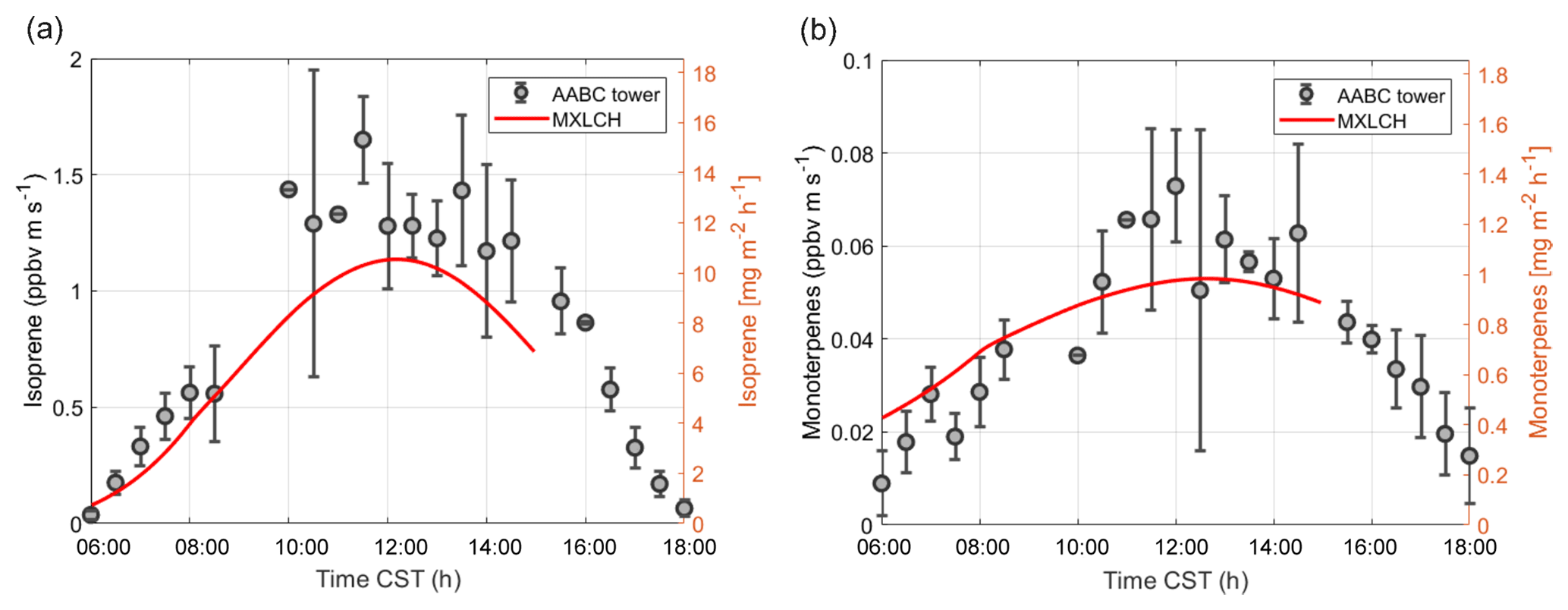
Figure 4Measured (black) and modelled (red) (a) isoprene and (b) monoterpene fluxes at the Alabama Aquatic Biodiversity Center (AABC) eddy covariance tower for 5, 6, 8, and 10–13 June 2013.
Figure 4 shows the interactively calculated above-canopy monoterpene and isoprene emissions (calculated from Appendix B). The isoprene flux falls in the lower end of the measurements (but within their uncertainties), while the monoterpene emissions are modelled accurately compared to the observations. The isoprene flux peaks at noon (at 1.1 ppb m s−1), while the monoterpene emission flux peaks at noon at just 0.05 ppb m s−1. The diurnal range of monoterpene emissions is small compared to isoprene (only 0.03 ppb m s−1) because monoterpene emissions depend only weakly on light (Emmerson et al., 2017). On the other hand, isoprene emissions respond to diurnal light availability (Guenther et al., 2006). Hence, the emission rates for isoprene are much more variable than emission rates for monoterpenes, as the model is run during the day with abundant light availability (measurements are chosen from clear days). Monoterpene emissions are mainly temperature dependent, and hence there is a slight increase towards noon (Holzinger et al., 2005). As outlined before, we speciate the monoterpene emissions as 45 % α-pinene, 45 % β-pinene, and 10 % limonene.
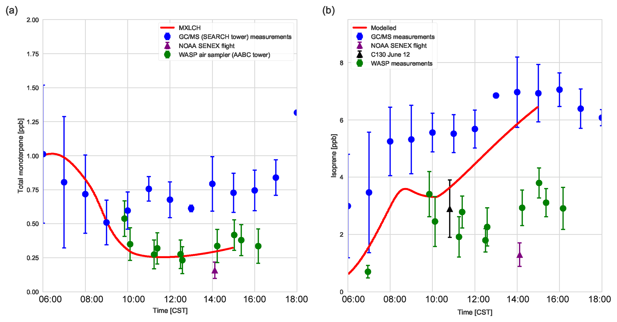
Figure 5(a) Total monoterpenes (sum of α-pinene, β-pinene, and limonene) and (b) isoprene measured above canopy (blue) above the SEARCH tower averaged from 5–13 June 2013; vertical profile measurements made by the NOAA SENEX campaign flight (purple) averaged for 11 June above the SEARCH super site, by whole air sample profilers (WASP; green and averaged for 5, 6, 8, and 10–13 June), and by the NCAR C-130 flight (black) on 12 June 2013 above the SEARCH super site. MXLCH-SOA model output in red. Error bars indicate 1 standard deviation. The WASP sampler only measured the bulk monoterpene mixing ratio instead of the speciated monoterpenes.
5.2 Diurnal evolution of BVOC mixing ratios
Figure 5a shows the mixing ratio of the bulk monoterpenes (sum of the mixing ratios of α-pinene, β-pinene, and limonene). The initial value is 1.0 ppb, which decays rapidly until 10:00, followed by an increase to just above 0.25 ppb at the end of the day. This shape of the monoterpene is reflected in the respective shapes of α-pinene, β-pinene, and limonene (see Fig. C2). The decay rate of the modelled monoterpenes is much higher than the surface observations (blue – SEARCH tower). The model underestimates the monoterpene mixing ratio compared to these ground observations (by about 0.5 ppb; almost by a third). These GC-MS measurements are taken on top of the SOAS tower, which is just above canopy height (20 m). The difference in the model and measurements might arise since the measurements are done within the roughness sub-layer, which is 3 times the canopy height (hc) (Vilà-Guerau de Arellano et al., 2015). The MXLCH-SOA model assumes a well-mixed ABL with a coupled surface layer model. However, concentrations closer to the surface fall within the roughness sub-layer and are usually different than in the mixed layer (Stull, 1988).
The mean values calculated from the vertical profiles of monoterpenes (made by SENEX above SEARCH; black and purple, Fig. 5a, and WASP above the AABC tower – green) indicate lower mixing ratios compared to surface (GC-MS) measurements (blue, Fig. 5a). These vertical profiles agree much better with the mixed layer approximation, with very good representation of the model with WASP air sampler measurements. As we are modelling the air above the canopy, airplane measurements give a good average of measurements in the atmospheric boundary layer, leading to better representativeness. The WASP air sampler only measures the bulk monoterpenes and not speciated monoterpenes, so a comparison per monoterpene cannot be made as in Fig. C2.
The isoprene mixing ratios (made by WASP and NCAR-130 above AABC; green and black, Fig. 5b) match well with the vertical profiles at the start of the day. However, they are overestimated in the late afternoon compared to the vertical profiles (green; boosted due to the high emissions calculated above the AABC tower; modelled 6.4 ppb, while measurements indicate 4 ppb ± 0.8 ppb) but are better matched to the isoprene mixing ratios measured at the SEARCH tower better (blue). The difference in measured isoprene mixing ratios indicates that isoprene is not very homogeneously well mixed in the horizontal or vertical, while the model assumes it is. In addition, model OH concentrations are in the low range of the observations in the afternoon, which could contribute to the overestimation of isoprene concentrations.
According to Su et al. (2016), ground-based measurements of species with short lifetimes (as is the case for monoterpenes and isoprenes) are not representative of the averaged concentrations inside the convective boundary layer (CBL). A short chemical lifetime could explain the disparity between the mixing ratio of the monoterpenes and isoprenes at the surface and measured in the vertical profile. According to Holzinger et al. (2005), the monoterpene concentration peaks in less well-mixed conditions (especially at night) and in more well-mixed conditions the monoterpene concentration falls. The oxidative lifetime of monoterpenes is relatively short; the monoterpene lifetime is between 18 and 48 min (Holzinger et al., 2005). Isoprene has a lifetime of approximately 1.4 h (Xu et al., 2015). However, these times are comparable with the turbulent mixing timescale, which is calculated as the boundary layer height divided by the convective velocity scale (w*). This velocity scale depends on the buoyancy of the air parcel and determines the time taken for the air parcel to reach the boundary layer (Vilà-Guerau de Arellano et al., 2015), which in this model is between 20 and 40 min and is comparable to the monoterpene lifetime.
In summary, within the limits of the measurements and observations, we obtained a reasonable representation of the diurnal evolution of gas-phase composition in a dynamically evolving boundary layer. Moreover, the evolution of other gas-phase mixing ratios is also reproduced within measurement range (Fig. C1). Next, we investigate the SOA concentration and diurnal evolution.
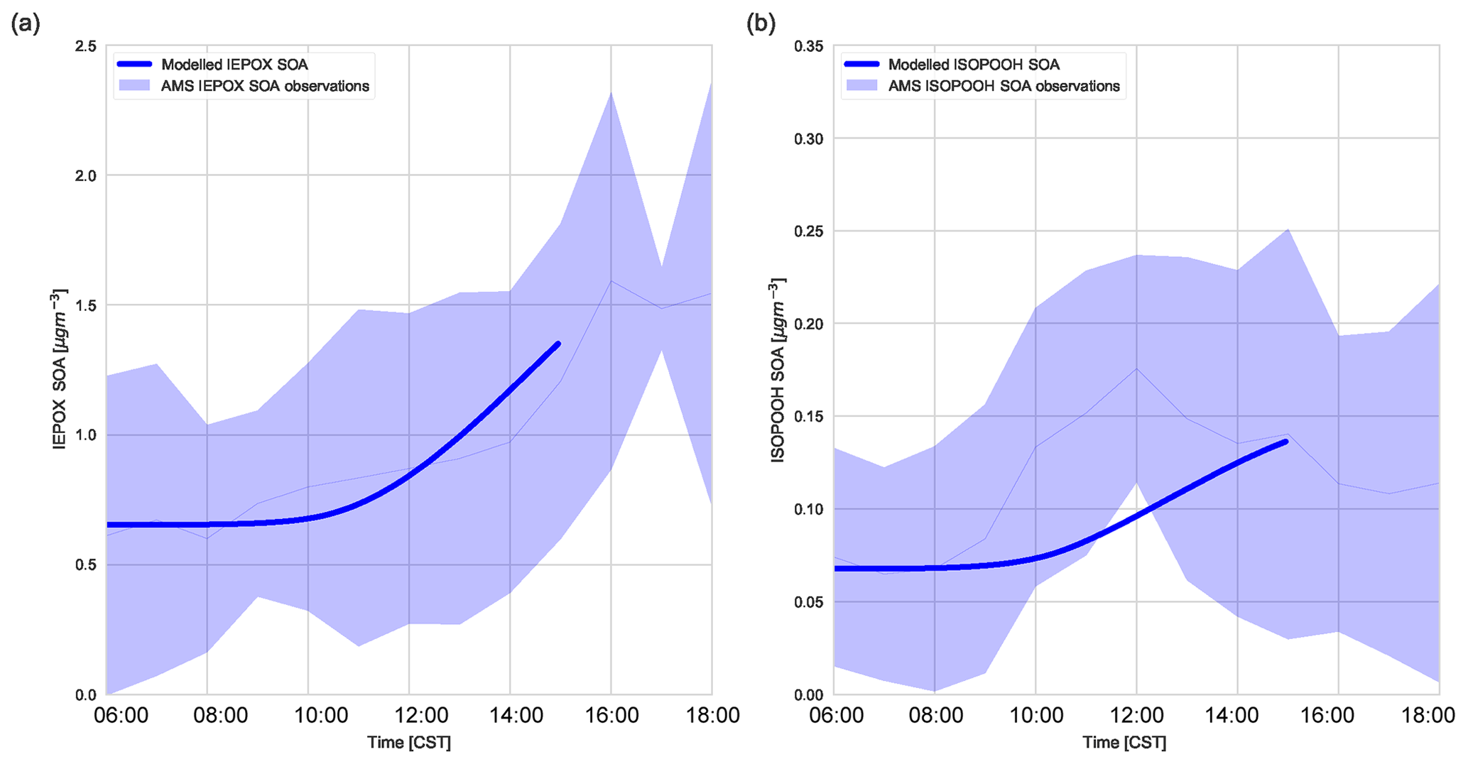
Figure 6(a) Diurnal IEPOX SOA evolution measured with aerosol mass spectrometry versus modelled IEPOX SOA and (b) diurnal ISOPOOH SOA evolution measured with aerosol mass spectrometry versus modelled ISOPOOH SOA above the SEARCH super site. The light blue shaded area represents the variability over these days (measurements averaged over 6, 8, and 10–13 June).
5.3 Diurnal evolution of isoprene SOA
Figure 6 shows that the model is able to capture the observed evolution of both IEPOX SOA and ISOPOOH SOA, which is similar to Hu et al. (2016) and Krechmer et al. (2015), respectively. The concentrations of IEPOX SOA and ISOPOOH SOA increase throughout the day, following the isoprene mixing ratio (Fig. 5b). At the end of the day the IEPOX SOA concentration is 1.45 µg m−3, while the ISOPOOH SOA concentration equals 0.155 µg m−3. There is a peak at noon in ISOPOOH SOA measurements, which matches Krechmer et al. (2015), but this peak is not captured by the model. ISOPOOH SOA formation depends on the OH concentration and hence the fast rise in ISOPOOH SOA coincides with the OH peak. ISOPOOH SOA is otherwise within the range of observations. IEPOX SOA formation is faster after noon due to a peak in OH concentration and isoprene emissions. From the ISOPOOH formed from this reaction, the branching ratio to IEPOX and ISOP(OOH)2 is approximately 88 % and 2.5 %, which results in a larger concentration of IEPOX SOA compared to ISOPOOH SOA (Krechmer et al., 2015). The mean isoprene SOA yield (the amount of IEPOX SOA and ISOPOOH SOA produced compared to the total isoprene chemical loss in the model) was calculated at 1.8 %, which is lower compared to the 3.3 % calculated by Marais et al. (2016) but well within the range of 1 %–6 % discussed by Krechmer et al. (2015).
The calculated γIEPOX in ambient SOAS conditions was 0.0087, and the subsequent heterogeneous reaction rate was calculated at s−1, which agrees with Hu et al. (2016). This value successfully models the observed IEPOX SOA. The IEPOX lifetime to uptake on acidic aerosol is relatively slow (timescale of approximately 5 h), though it depends on the time of the day. pH is low in the afternoon and this accelerates uptake (Krechmer et al., 2015). We use a pH of 0.8 (corresponding to Hu et al. (2016) wherein the H+ proton concentration was 0.15 M for the ambient case), though as we do not include diurnal variation of pH in this model, the diurnal effect is not captured in the model. The relatively slow uptake implies that dry deposition and OH reaction compete significantly with the heterogeneous uptake of IEPOX, as concluded in prior studies (Hu et al., 2016; Nguyen et al., 2015a). The budget contribution of IEPOX SOA to total SOA is small in the first 3 h of the day and picks up in the latter part of the day, which follows the isoprene peak. The rate of IEPOX SOA formation peaks at 14:00 CST, with the steepest increase between 10:00 and 12:00 CST. Once formed, IEPOX SOA is thought to have a relatively long lifetime (1–2 weeks against wet deposition, 2 weeks through heterogeneous OH reaction; Hu et al., 2016).
5.4 Constraining the SOA budget at SOAS: model versus observations
Figure 7 shows the diurnal evolution of the measured total SOA (and the contribution of each observed factor) against the modelled IEPOX SOA, ISOPOOH SOA, and the modelled total SOA (as a sum of IEPOX SOA, ISOPOOH SOA, and MT SOA). The light blue shaded area shows the variability over the days averaged for the aerosol measurements, and the modelled diurnal evolution of the SOA falls within this standard deviation. The modelled SOA concentration remains relatively constant in the early morning, as is reflected by the SOA observations. The modelled SOA concentration then decreases as it is diluted by the ABL growth as entrainment mixes in air with a lower SOA concentration. The modelled SOA concentration increases towards the end of the day, driven by the rise in ISOPOOH and IEPOX SOA concentrations, reaching 3.5 µg m−3 by the end of the day.
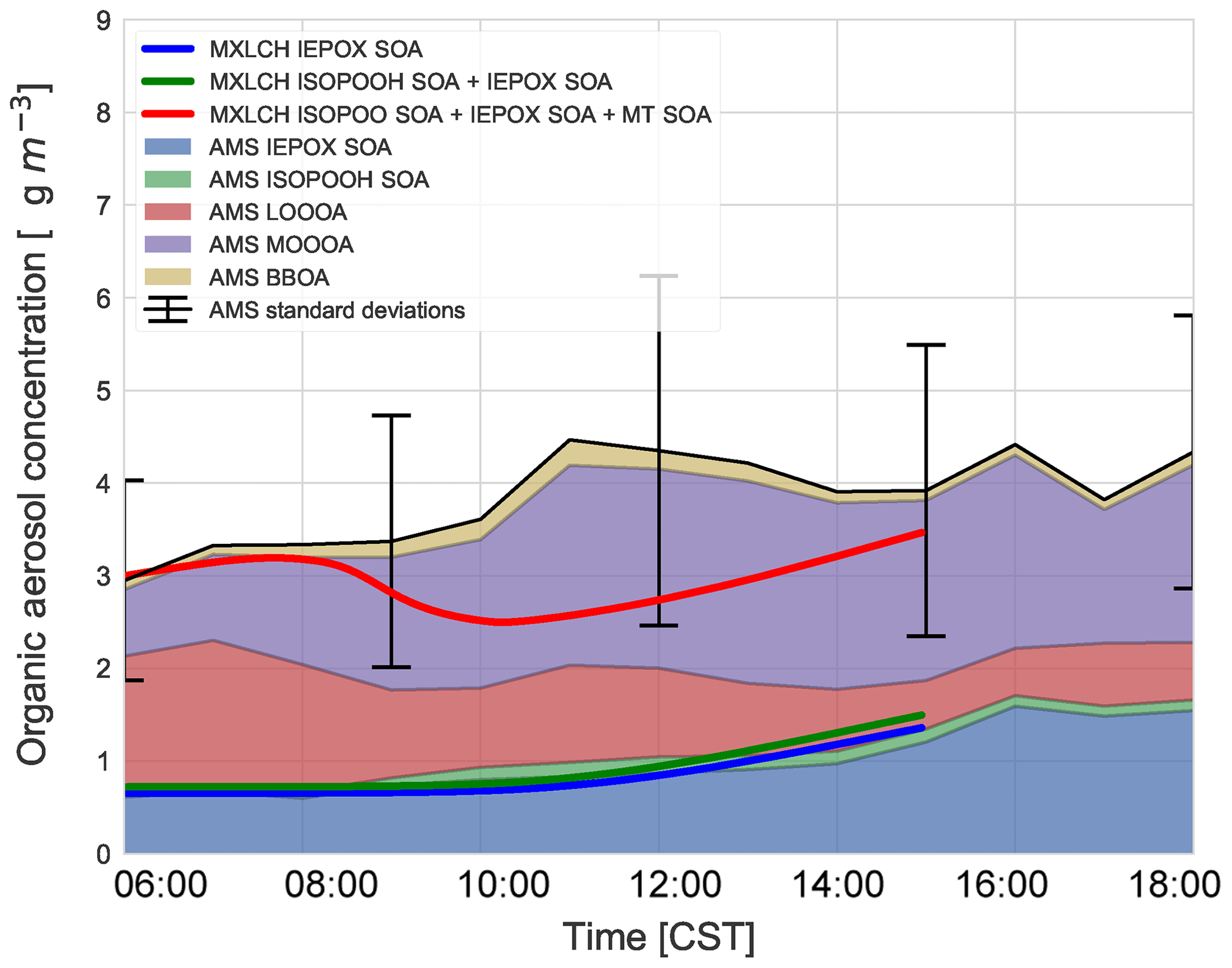
Figure 7SOA measured at the SOAS site versus SOA modelled in the MXLCH-SOA model. The observations are averaged over 6, 8, and 10–13 June 2013 and show the stacked contribution of IEPOX SOA, ISOPOOH SOA, LO-OOA, MO-OOA, and BBOA, which made up the majority of the aerosol mass at the SOAS site. The light blue area shows 1 standard deviation of the total SOA measurements. The solid lines show the SOA modelled in MXLCH-SOA, with the blue line showing IEPOX SOA; green shows IEPOX SOA + ISOPOOH SOA and the red line shows the total SOA (IEPOX SOA + ISOPOOH SOA + MT SOA) formed in the model.
According to the model, the largest contribution to SOA comes from the gas–aerosol partitioning of monoterpene oxidation products, approximately between 73 % in the morning and 58 % by the end of the day with a mean of 69 %. This monoterpene SOA can be compared to the LO-OOA and MO-OOA measurements, though MO-OOA is assumed to be more aged and could either be left over from previous days (entrained from the RL) as a result of advection, in which case it is not locally produced and represents a regional concentration (Jimenez et al., 2009; Xu et al., 2015), or a result of fast oxidation (and hence locally produced). MT SOA is formed via gas–particle partitioning and Fig. C3 shows the partitioning that takes place in each of the four bins in the VBS.
Based on PMF source apportionment, LO-OOA and MO-OOA contributed 33 % and 39 %, respectively, to ambient total SOA in the southeastern US (Xu et al., 2015). Hence, throughout the campaign a major part of SOA is LO-OOA and MO-OOA in the southeastern US and hence a large part of SOA formed in the model can be attributed to G–P partitioning. As the majority of the G–P partitioning is monoterpene based, MT SOA contributes significantly to total SOA formation in the southeastern US (Ayres et al., 2015; Zhang et al., 2018). The addition of nitrate reactions can also make a significant contribution to the SOA fraction (Ayres et al., 2015); however, this is not the case in our model, as observed in Fig. C6.
The model, which predicts locally formed OA only, bisects MO-OOA between 09:00 and 15:00 (Fig. 7), implying that there is some aged SOA in the system (more than 1 µg m−3 in the system at 11:00). In the morning, as there is not much OH history, the aged MO-OOA could be from the previous day and entrained into the ABL from the FT. In the afternoon, the ABL stops growing and is deeper such that local effects become more dominant. Local partitioning of SVOC contributes between half and the majority of the MO-OOA in the afternoon, which could indicate that aerosol becomes more aged over the day in approximately 4 h. It would be instructive to study changes in the composition of the species comprising MO-OOA with more molecularly specific analysis methods and check whether this change over the day is consistent with a shift from aged to rapidly oxidised local products or whether it is just an identical product mixture from a different region. This might address the issue of aged SOA transported in versus fast local oxidation. Most importantly, however, the model and measurements agree on 3–4 µg m−3 of afternoon SOA during the SOAS campaign.
A bulk budget analysis can be used to differentiate the contribution of entrainment and the different SOA factors to the SOA budget. The entrainment budget for background OA is calculated as per Janssen et al. (2012):
in which the entrainment flux is calculated from the entrainment velocity (we in m s−1), the concentration jump in background OA (ΔOABG in µg m−3) between the RL and BL, and the boundary layer height (h in m).
From Fig. 8, we can determine the contributions of different processes and chemical species to total SOA. The early morning SOA consists primarily of MT SOA (formed by gas–particle partitioning) as per Fig. 7. The contribution of entrainment to the total rate of change of the SOA concentration peaks at 09:00, when entrainment contributes more than 86 % to the total SOA tendency. Hence, as the boundary layer height is growing the fastest (Fig. 3) and the entrainment velocity is also peaking (0.12 m s−1 at 09:30), the SOA concentration decreases due to the introduction of SOA-poor air from the RL. Just after 10:00 CST, the effect of entrainment is low and hence the SOA tendency becomes positive again, as production picks up from a sum of IEPOX SOA, ISOPOOH SOA, and MT SOA from G–P partitioning. By the late afternoon, IEPOX SOA has the largest contribution to the SOA budget (68 %), while the contribution of MT SOA decreases (to 27 %) at this time, as the contributions of α-pinene, β-pinene, and limonene are lower in the afternoon. The mixing ratios of monoterpenes decrease due to entrainment in the early morning and strong reaction with OH, which peaks around noon, while the emissions, though continuous, are unable to compensate for the increased oxidation and entrainment; therefore, the monoterpene contribution to SOA later in the afternoon is smaller. ISOPOOH SOA has a very small contribution to the SOA budget (end-of-day contribution 3.9 %).
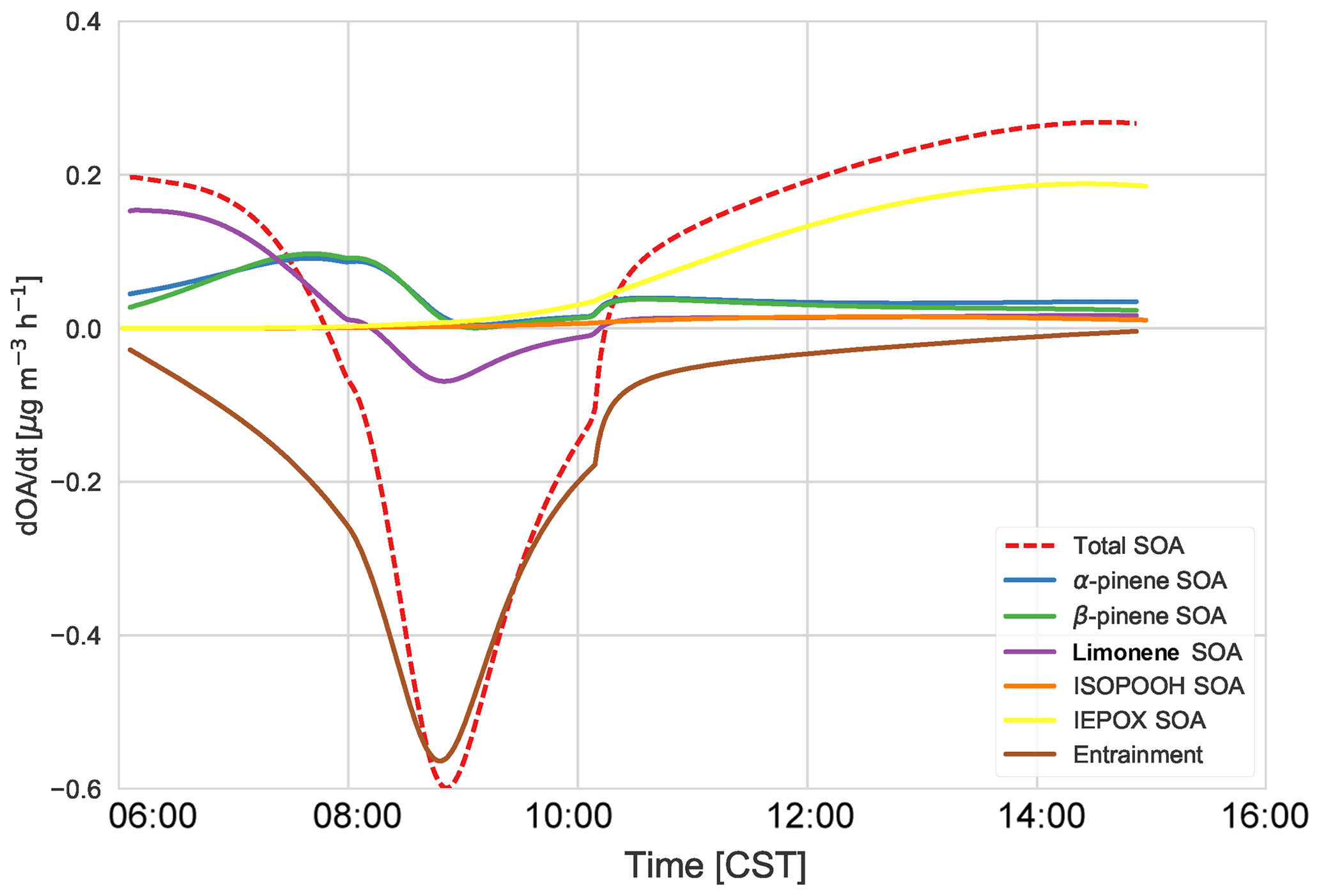
Figure 8The SOA budget, which consists of the total tendency (dashed) and the contribution from entrainment of background OA (pink). The chemistry contribution is split into IEPOX SOA (yellow), ISOPOOH SOA (orange), α-pinene SOA (red), β-pinene SOA (blue), and limonene SOA (green). The total MT SOA (purple) is just the sum of α-pinene SOA (red), β-pinene SOA (blue), and limonene SOA (green).
α-Pinene contributes about 18 % of the total SOA, while β-pinene contributes about 10 % in the early morning. The contribution of both rises, and by 08:00 MT SOA is largely from α- and β-pinene (α-pinene and β-pinene are approximately 50 % each). By the end of the day, α-pinene SOA dominates, contributing about 50 % to MT SOA and 12.5 % to the total SOA. Rather surprisingly, the limonene product dominates the SOA contribution in the morning (approximately 60 %). This is surprising as the limonene mixing ratio is much lower than α- and β-pinene (Fig. C2). However, as discussed in previous literature (Krechmer et al., 2015; Lee et al., 2006), the limonene SOA yield is much higher than the yield of α-pinene and β-pinene. The stoichiometric coefficients for limonene + OH and O3 are also higher than the OH and O3 + α- and β-pinene stoichiometric coefficients. As there is an OH peak in the morning in the shallow boundary layer and the oxidation reactions between limonene and OH and O3 are fast (Table A6: R44, R45), this results in a large accumulation of limonene SOA product in the morning. As the boundary layer grows, entrainment dilutes this product, causing a fall in the limonene SOA tendency. As the day progresses the contribution of limonene SOA becomes less dominant (6 % by the end of the day) and the α- and β-pinene contributions become more important. The isoprene + O3 and NO3 pathways lead to a negligible amount of SOA formed in our model, even in the early morning. The early morning NOx chemistry and subsequent SOA formation are constrained through the observed NO and NO2 initial mixing ratios. Since the resulting NO3 (and N2O5) mixing ratios are very small, the NO3-initiated SOA formation is negligible. The oxidant + BVOC pathway contribution can be seen in Fig. C6; OH oxidation is the most important contributor to aerosol formation.
To test the sensitivity of the coupled land surface–boundary layer–SOA formation system, we carried out numerical experiments on the initial conditions of the model. We evaluated the effect of the initial RL concentration of SOA on the diurnal evolution of SOA in the ABL.
These experiments are guided by measurements of SOA concentration above the boundary layer at 11:00 CST from the SENEX flights (Fig. C4). We use the range of these profile measurements as constraints on the numerical experiments. In the previous section, we discussed the entrainment of aged SOA from previous days from the RL into the mixed layer as the boundary layer grows. Figure 9 shows the sensitivity of diurnal SOA evolution in the boundary layer to the concentration of background SOA in the RL. We constrain SOA concentrations by the vertical profiles from by the SENEX flights (Fig. C4 and Wagner et al., 2015) and a case in which the concentration of SOA is the same in the ABL and RL at the start of the simulation. We compare the effect of the RL SOA concentration on the modelled SOA against the observed SOA concentrations.
We find that a uniform SOA concentration in the ABL and RL no longer leads to a drop in SOA due to growth of the ABL, but leads to overestimated values compared to the observations during the end of the afternoon. In cases in which the concentration of SOA is less in the RL than the ABL, there is a dilution of SOA as the boundary layer grows, as entrainment mixes air with less SOA from the RL. This is more marked when the concentration difference is larger. This difference is also found by Janssen et al. (2012, 2017), who discussed the importance of background OA concentration in the RL; if there is a large jump of background OA between the ABL and RL it has a significant effect on diurnal SOA evolution. Tracer concentrations are generally lower in the RL compared to the ABL (which is the case for SOA in Fig. C4), and hence entrainment dilutes the concentrations in the ABL (Karl et al., 2007, 2009). In order to accurately understand diurnal SOA evolution, it is very important to have a good estimate of its RL concentration in the early morning.
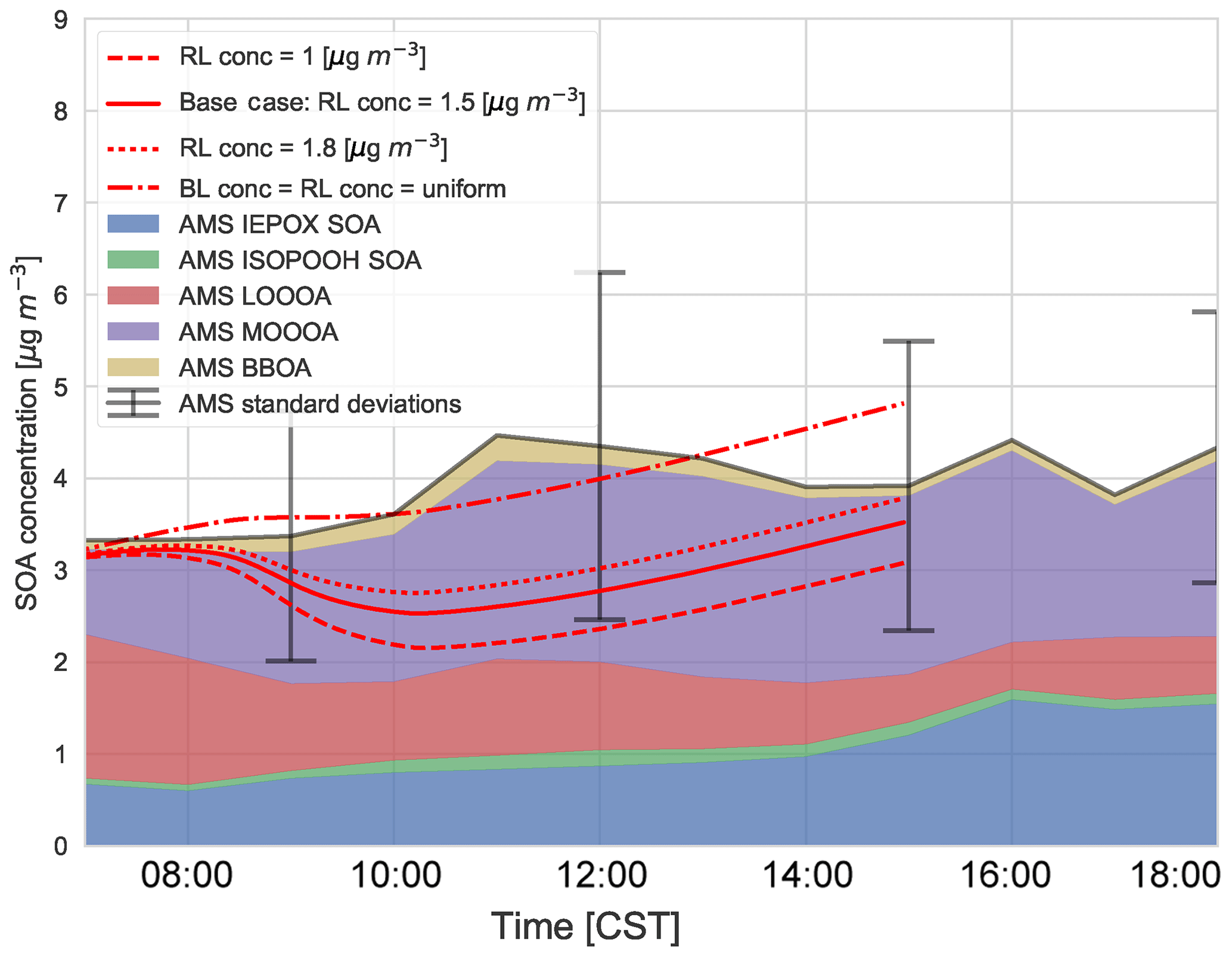
Figure 9Sensitivity of the diurnal SOA evolution to initial free tropospheric organic aerosol (OABG) compared to the (average) AMS observations of IEPOX SOA, ISOPOOH SOA, LO-OOA, MO-OOA, and BBOA averaged over 5, 6, 8, and 10–13 June 2013. “BL conc” and “RL conc” indicate the concentrations in the boundary layer and residual layer, respectively.
This sensitivity analysis also provides an opportunity to allocate the source of SOA. As SOA is relatively long-lived, the amount of aged SOA in the RL can have a large effect on the SOA in the ABL, as it affects the vertical mixing of SOA and SOA availability for G–P partitioning. The drop in measured LO-OOA concentrations (in the morning) indicates a dilution that is driven by entrainment as LO-OOA-poor air is introduced into the BL from the RL. If we consider a uniform concentration in the ABL and RL, most of the MO-OOA is captured by the model (implying the dominance of local production), though there is an overestimation of SOA formation in the early morning and late afternoon (although the model results are within 1 standard deviation of the measurements and within measurement uncertainties). The more oxidised oxygenated organic aerosol (MO-OOA) could result from entrainment from the RL, though the available measurements show that the OA concentration in the RL is between 1 and 1.8 µg m−3 (Fig. C4 and Wagner et al., 2015), so not all the aged MO-OOA can be explained by this process and some must be horizontally advected. In addition, the rapid formation of MO-OOA via autoxidation reactions (Ehn et al., 2014) or the substantially lower volatility of ambient SOA compared to that assumed in VBS-based models (Hu et al., 2016; Stark et al., 2017) may contribute to explaining the model–measurement differences in MO-OOA when the experimentally constrained RL concentrations are used in the model.
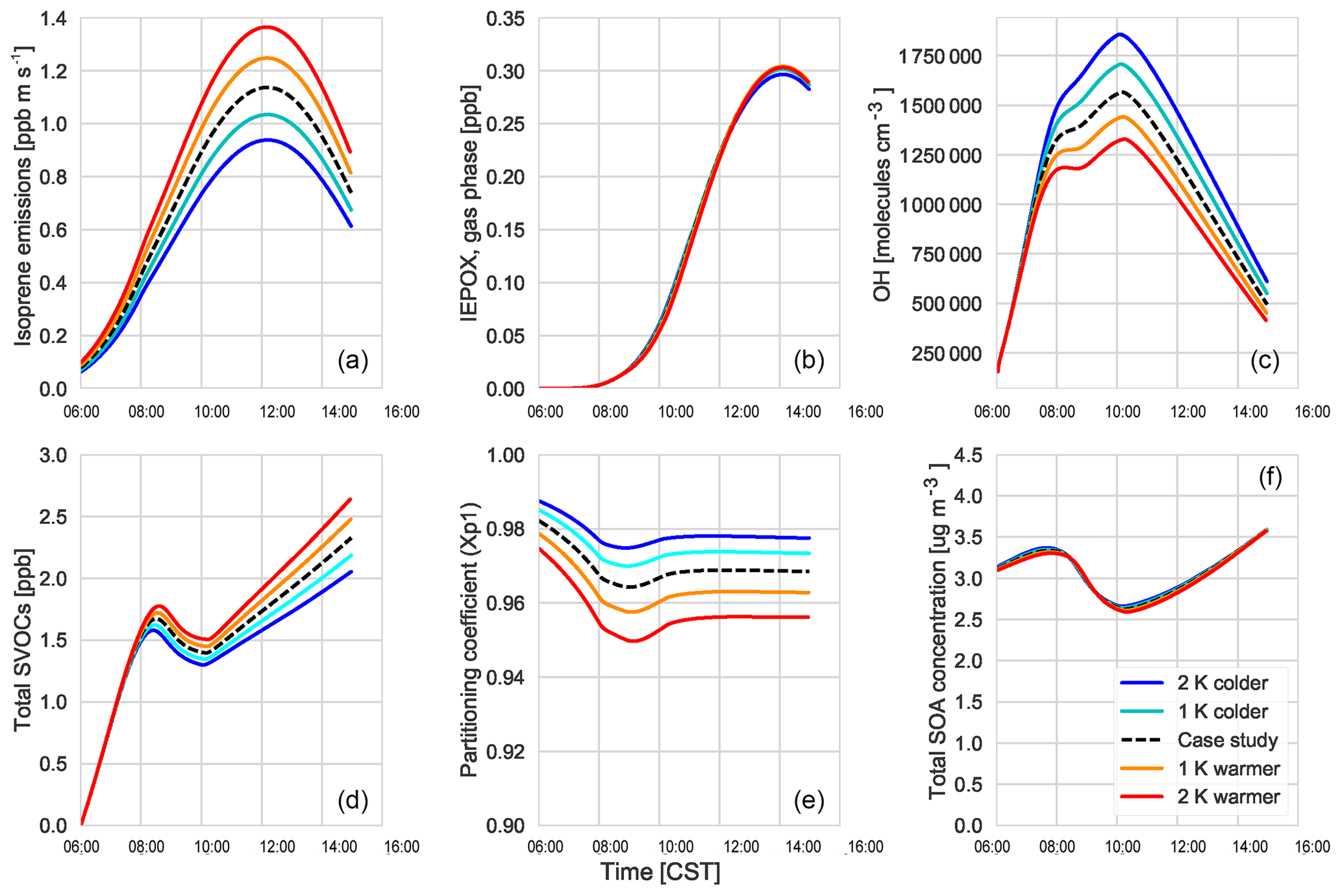
Figure 10The response of isoprene emissions (a), gas-phase IEPOX mixing ratios (b), OH (c), total SVOC mixing ratios (d), partitioning efficiency in the first volatility bin (e), and the total SOA concentration (f) to changing temperatures.
Using our coupled land surface–boundary layer–SOA formation model, we can study the net effect that temperature has on SOA concentration through VOC emissions, G–P partitioning, and feedbacks between the ABL and the land surface that influence entrainment of SOA from the residual layer. In our experiments, in which we varied the early morning temperature by between −2 and +2 K, we find that the total SOA concentration in the daytime ABL is buffered against temperature changes (Fig. 10).
Isoprene (Fig. 10a) and monoterpene emissions (Fig. C5d) are temperature dependent (Guenther et al., 2006), and consequently we observe a positive impact of rising temperature on these BVOC fluxes. At higher temperatures, this means there is an accumulation of BVOCs in the ABL, which consequently leads to a depletion of OH (Fig. 10). However, as we do not take OH recycling into account in the oxidation of isoprene, this has an effect on OH depletion. The change in the IEPOX gas-phase mixing ratio (Fig. 10) is not as large as the isoprene emissions as a consequence of the depletion of OH and slower reaction rates compared to BVOCs. Consequently, the effect of temperature on IEPOX SOA is rather small, with a minuscule increase in IEPOX SOA formed at higher temperatures at the end of the day (around 0.02; Fig. C5).
The abundance of BVOCs leads to a build-up of SVOCs in the ABL that are available for partitioning, but since partitioning to the aerosol phase is generally favoured at lower temperatures, rising temperatures reduce the partitioning coefficient (Takekawa et al., 2003). Janssen et al. (2012) discussed the fact that the partitioning efficiency of SOA had a non-linear response, especially at low temperatures and high background SOA availability. At low OABG concentrations and high temperatures, the partitioning coefficient is small; however, there is a slight increase in SOA concentration.
A rising temperature could, in principle, affect surface heat fluxes and ABL development by increasing the vapour pressure deficit (Van Heerwaarden et al., 2009). However, we find that for a temperature increase of 2 K, this effect is of minor importance (Fig. C5), and the entrainment of SOA is hardly affected. Overall, a rise in temperature does not have a significant effect on modelled SOA concentration.
However, the southeastern US, in contrast to the rest of the US, has experienced cooling summer temperatures which have been linked to either high aerosol loading or other large-scale synoptic meteorology predominant in that region (Goldstein et al., 2009; Pan et al., 2013). Cooler temperatures favour partitioning to the aerosol phase, although BVOC emissions will be lower. If the concentration of aerosol is already high, however, the low temperatures would lead to an increase in aerosol concentration. The regional cooling caused by the high aerosol concentration could further exacerbate this situation. The decrease in temperature by 1 and 2 K shows that SOA concentrations do not change much despite the decrease in available BVOCs. This means that the cooling that has been seen over this region of the US is unlikely to have affected SOA concentrations above the region.
The radiative effect caused by high aerosol loading means that the region is likely to stay cooler than the rest of the US (Barbaro et al., 2014; Goldstein et al., 2009), which should increase aerosol in the regions, though at cooler temperatures the BVOC emissions will be lower, which would limit SOA formation. These radiative effects of aerosol on the surface energy balance (Barbaro et al., 2014) are, however, not included in this work.
The coupled land–atmosphere model gives us the ability to explore the sensitivity of SOA formation to different variables that might change in the future due to changing climate regimes. It would be interesting, for instance, to study the effect of drier or wetter climates on SOA diurnal variability.
We studied the diurnal evolution of biogenic secondary organic aerosol formed from daytime sources in the southeastern US by combining the MXLCH-SOA model with observations from the SOAS campaign. By coupling the MXLCH-SOA boundary layer–chemistry model to modules that interactively calculate surface VOC fluxes and heat fluxes, we can study diurnal SOA evolution in the context of a tightly coupled land surface–boundary layer–SOA formation system.
An evaluation with observations shows that our model system reproduces observations of surface fluxes, tracer concentrations, and boundary layer height satisfactorily. Deviations from observed mixing ratios were found for isoprene and monoterpenes measured just above canopy. However, modelled mixing ratios of VOCs agree better with aircraft observations, which are actually more representative for the mixed layer.
We considered several mechanisms for SOA formation from isoprene and monoterpenes, though the model was limited to daytime, and night-time SOA formation was not included. Reactive uptake of IEPOX SOA agreed well with observations, thereby corroborating previous studies, in a case study that is tightly constrained by observations. ISOPOOH SOA formation though condensation is reproduced within the measurement uncertainty, although the observed peak around noon is not captured by the model. The mean isoprene SOA yield is 1.8 %, which is in the lower range of values reported in the literature.
MT SOA dominates over isoprene SOA, contributing 68 % to aerosol mass, with limonene having the largest contribution in the early morning (60 %) and α-pinene and β-pinene during the rest of the day. The mean MT SOA yield is 10.7 %. In contrast to isoprene SOA, there are no observed monoterpene-specific aerosol factors, so both the LO-OOA and the MO-OOA factors may result from MT SOA formation. Our findings suggest that the more oxidised oxygenated organic aerosol (MO-OOA) could result from entrainment from the residual layer in the late morning and fast autoxidation reactions in the late afternoon, although the roles of horizontal advection and/or lower real MT SOA volatility than in the VBS used here may also play a role in the observed differences. VOC oxidation by the nitrate radical contributed negligibly to SOA formation during daytime, while OH-initiated reactions dominated SOA formation. Overall, the relatively flat diurnal cycle of the total observed SOA can be explained by the contrasting effects of local SOA production and entrainment of SOA-depleted air from the residual layer.
In a sensitivity analysis of the coupled land surface–boundary layer–SOA formation system to temperature changes, we find that the effect of increasing BVOC emissions with increasing temperatures is offset by a depletion of OH concentrations and a decrease in the partitioning efficiency of SVOCs into the aerosol phase. This suggests that near-surface SOA concentrations in the southeastern US are buffered against temperature changes in the region. The use of a fully coupled land surface–boundary layer model that enables the interactive calculation of surface heat and entrainment fluxes makes it possible to study how VOC fluxes, heat fluxes, and ultimately SOA concentrations respond to changing forcings.
The MXLCH-SOA code is available at http://classmodel.github.io/ (last access: January 2019). The data sets used in this work are available from the cited references.
Table A1Dynamics: initial and boundary layer conditions to reproduce the dynamical properties of 11 June 2013 from the SOAS measurement campaign based on Su et al. (2016).
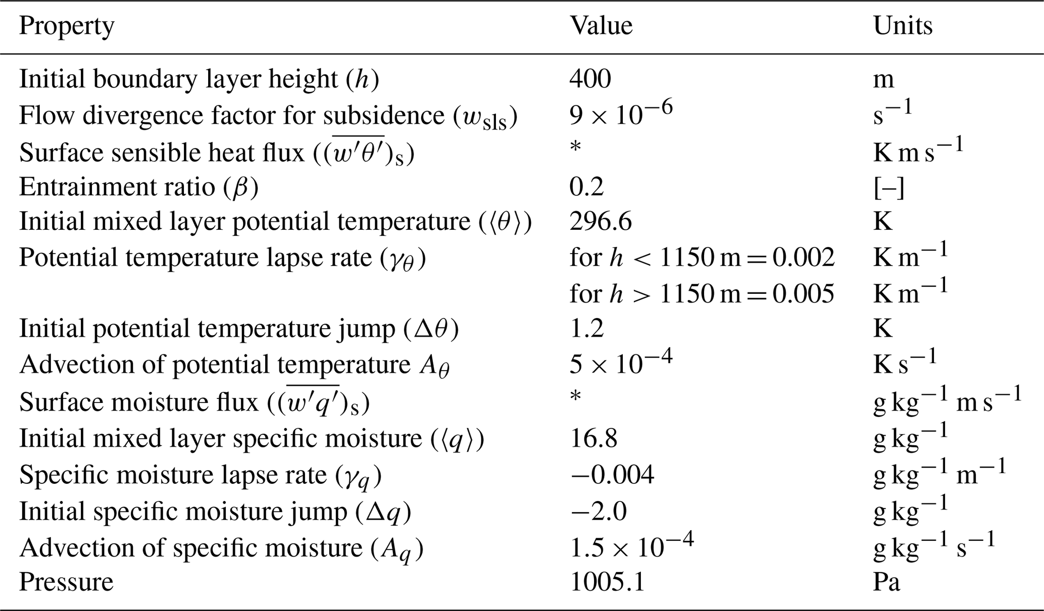
* Calculated interactively in Sect. 3.4.
Table A2Chemical reaction scheme. In the reaction rates, T is the absolute temperature in Kelvin and χ is the solar zenith angle. First-order reaction rates are in s−1, and second-order reaction rates are in cm3 molecule−1 s−1. PRODUCTS are the species which are not further evaluated in this chemical reaction scheme. The reaction scheme is derived from Janssen et al. (2013) and Su et al. (2016) and new reactions adapted from Hu et al. (2016), while speciated monoterpene reactions and reaction rates are from Orlando and Tyndall (2012), Crounse et al. (2011), and Atkinson and Arey (2003). SVOCs are shown in bold, which are then distributed per bin and multiplied by the respective α factor.
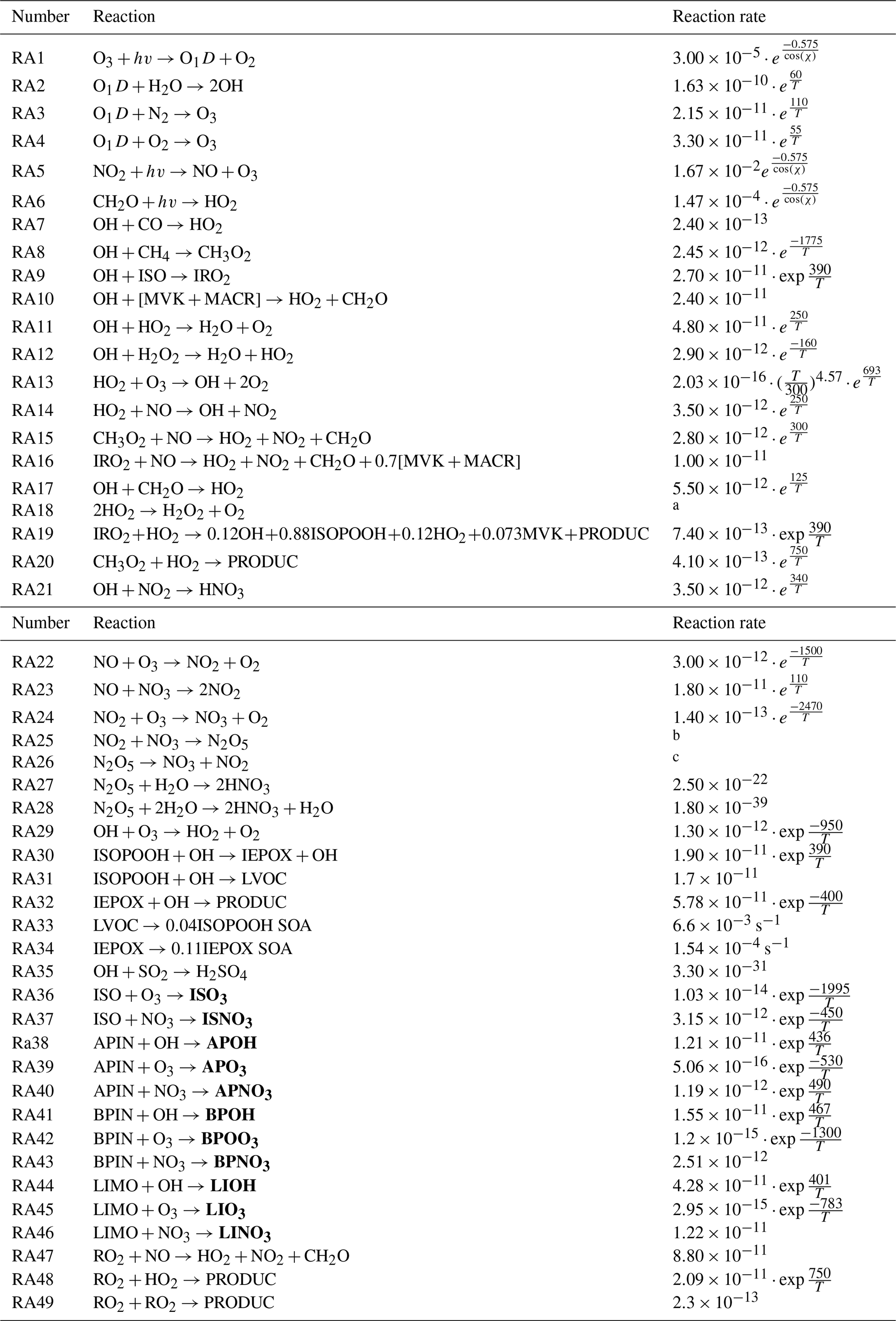
a ; ; . b ; ; . c ; ; .
Table A3Stoichiometric coefficients for different volatility bins for the precursors α-pinene (APIN), β-pinene (BPIN), limonene (LIMO), and isoprene (ISO) and depending on the oxidant (OH, NO3, and O3) at 298 K. ISO+OH is not considered as this is included in the reactive uptake and condensation pathways, and the ISO+NO pathway is not considered due to the low NOx availability in this region. Saturation concentrations, , are in µg m−3 and based on Pye et al. (2010).
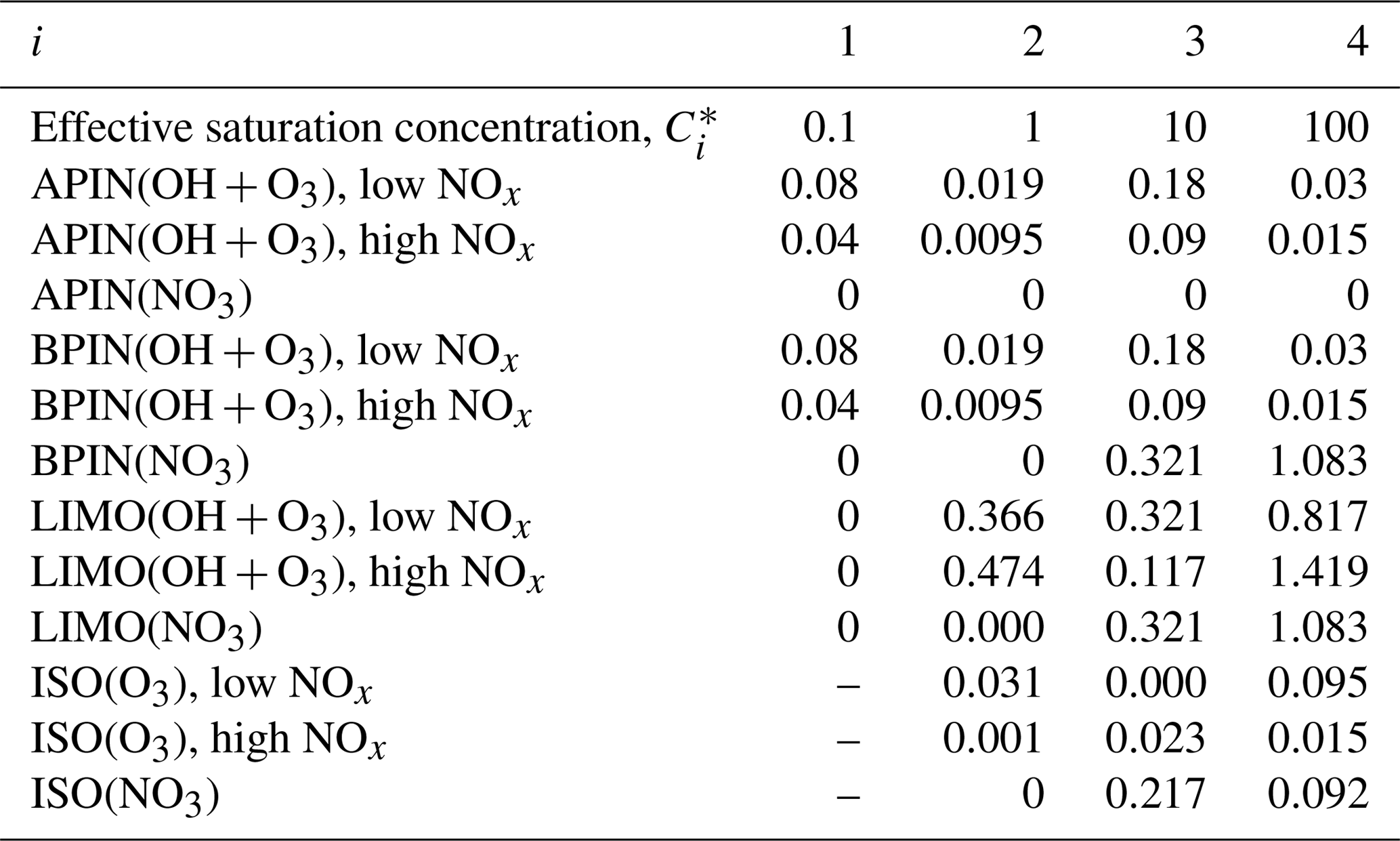
Table A4Advanced surface variables: plant and soil initial and boundary layer conditions to study the effect of a coupled land–atmosphere scheme. The plant scheme has been taken from the Van Heerwaarden et al. (2009) value for the broadleaf tree (deciduous forests) sand loam soil, with some observations taken from the Integrated Surface Flux System measurements taken at the AABC flux tower.
* Clapp and Hornberger retention curve parameter.
Table A5MEGAN parameters and values used in the mixed layer model.
a Above-canopy photosynthetic photon density flux. b Photosynthetically active radiation in W m−2. c Daily mean of above-canopy photosynthetic photon density flux.
Table A6Initial mixing ratio in the atmospheric boundary layer (ABL) and free troposphere (FT); surface emission–deposition fluxes of reactants based on Su et al. (2016). Gas-phase chemistry conditions are based on ground observations at SEARCH site, flux tower observations at the AABC tower, and aircraft observations (WASP system and NCAR-130 flight) and then averaged for 5, 6, 8, and 10–13 June (Su et al., 2016). Observations for secondary organic aerosol are from the aerosol mass spectrometer on the SEARCH ground site and a SENEX flight on 11 June. Species with 0 initial concentrations and emissions are not included in the table. The SVOCs have a 0 initial concentration but a deposition velocity of 0.024 m s−1 (not mentioned in the table).

a Dry deposition velocity in m s−1. b Interactively calculated in Sect. 3.3. c The OA is converted to µg m−1 in the model using a molecular weight of 250 g mol−1 multiplied by the pressure (Pa), divided by the gas constant R (8.3145 J mol−1 K−1) and the potential temperature (K) at half the boundary layer height, all multiplied by 0.001 (to convert it to µm).
This parameterisation is based on Guenther et al. (2006). In this model, the emissions, E, of isoprene and other BVOCs are parameterised by
Here, [ϵ] represents the base emissions in µg m−2 h−1 of a compound, while ρ accounts for the production and loss of the BVOC within canopy, which for isoprene is set to 0.96 (Guenther et al., 2006). The base emission rates are dependent on the plant functional type, and since we are over a broadleaf forest the emission rate for isoprene is set at 3000 µg m−2 h−1 (= 0.83 µg m−2 s−1); though it is low for a broadleaf area it is used as it is able to reproduce the isoprene mixing ratio observations. γ (dimensionless) is an emission activity factor and represents variation in emissions due to changes from standard conditions. It is derived for isoprene per
γ is a lumped correction factor (Wang et al., 2017); it takes into account the effect of the canopy environment γCE, the leaf age γAge, and soil moisture γSM.
A constant value for γAge is used (γAge=1). In order to calculate γCE, we utilise the parameterised canopy environment emission activity (PCEEA) algorithm. This is calculated by
The parameterised γ values are activity factors that are related to variations of temperature (t), light, and the leaf area index (LAI) (Guenther et al., 2006); γT is temperature dependent, and γLAI depends on the leaf area index, while γP represents the leaf-level photosynthetic photon flux density (PPFD), with units in µmol m−2 s−1. The PPFD is related to photosynthetically active radiation (PAR) (Guenther et al., 2006). PAR is the radiation that organisms can use for photosynthesis, and in our model framework the PAR depends on the incoming solar radiation.
Isoprene emissions respond to changes in PPFD at canopy level by
where a is the solar angle (calculated by subtracting the zenith angle from 90∘) in degrees. Pdaily is related to the PAR (multiplied by 4.766 to convert it from W m−2 to µmol m−2 s−1) and represents the daily mean of the above-canopy PPFD, and ϕ is the transmission of the above-canopy PPFD, which is non-dimensional (Guenther et al., 2006) and approximated by
The Pac, the above-canopy PPFD, is also approximated from PAR multiplied by a conversion factor (4.766). Ptoa, the top of the atmosphere PPFD (Guenther et al., 2006), depends on the day of the year (DOY).
The response of isoprene emissions to temperature is calculated by
Here , CT1 (= 80), and CT2 (= 200) are empirically derived coefficients, and Topt is the optimal temperature at which Eopt is calculated (Guenther et al., 2006).
Tdaily is the representative daily average air temperature at canopy level for the modelling period (K), which is set to 298 K based on surrounding temperature measured at the SOAS campaign site. Lastly, for canopy level, the isoprene emission dependence on the leaf area index (LAI in m3 m−3) is estimated by
The last γ factor, γSM, is 1 if the soil moisture θ is greater than θl, 0 if θ is less than the wilting point θw, and if θw is less than θ, which is less than θl; Δθl is an empirical parameter equalling 0.06 (Guenther et al., 2006).
For the monoterpene flux, in Eq. (B1), ρ=1 and ϵ=850 µg m−2 h−1 to fit the monoterpene mixing ratio observations, and γ is given by
As above, it is determined by the canopy emission activity factor and the soil moisture emission activity factor. The soil emission factor, however, is only considered for isoprene, and not other BVOCs in the MEGAN model, and hence for monoterpenes is set at 1 (Guenther et al., 2012; Sakulyanontvittaya et al., 2008). The canopy emission activity factor is calculated by
which depends on the LAI emission activity factor, γLAI, and the temperature emission activity factor, γT. The γLAI is also 1; however, the temperature emission activity factor is approximated by
Here βMT is the beta (an empirical coefficient) for monoterpene, set at 0.1 K−1 (Guenther et al., 2006), Ts is the skin temperature, and Tref is the reference temperature for the BVOC base emission rate (K) and equals 303 K.

Figure C1(a) Ozone, (b) nitrogen oxide, (c) nitrogen dioxide, and (d) hydroxide (OH) mixing ratio measured (blue) at the SOAS super site versus modelled by the MXLCH-SOA model (red) over the SOAS super site during the SOAS measurement campaign for the days 5, 6, 8, and 10–13 June 2013.
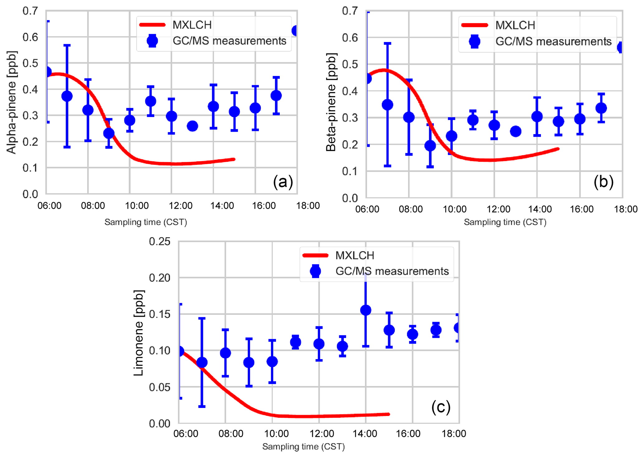
Figure C2Mixing ratios of (a) α-pinene, (b) β-pinene, and (c) limonene measured (blue) by gas chromatography–mass spectrometry over the SOAS super site tower (20 m above canopy), averaged over 5–13 June 2013, versus the mixing ratios modelled (red) in the MXLCH-SOA model.
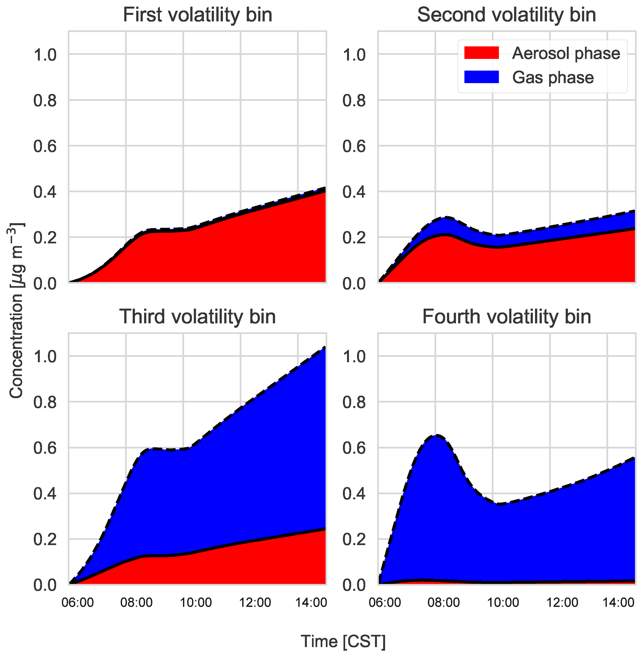
Figure C3Gas–particle partitioning products per volatility bin, with red indicating the amount of SVOC in the aerosol phase versus the gas phase (blue).
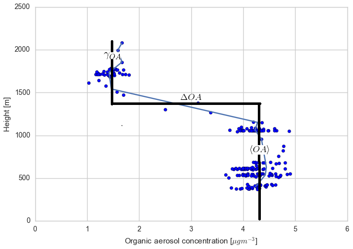
Figure C4Measured vertical profile of organic aerosol (blue dots) taken during the SENEX campaign above the SOAS campaign sites on 11 June 2013 at 14:00 CST, averaged for different heights (blue line) and overlaid with a typical convective boundary layer vertical profile: a mixed layer represented by a bulk value (〈OA〉), a sharp discontinuity in the inversion layer (ΔOA), and a value in the free troposphere (γOA).
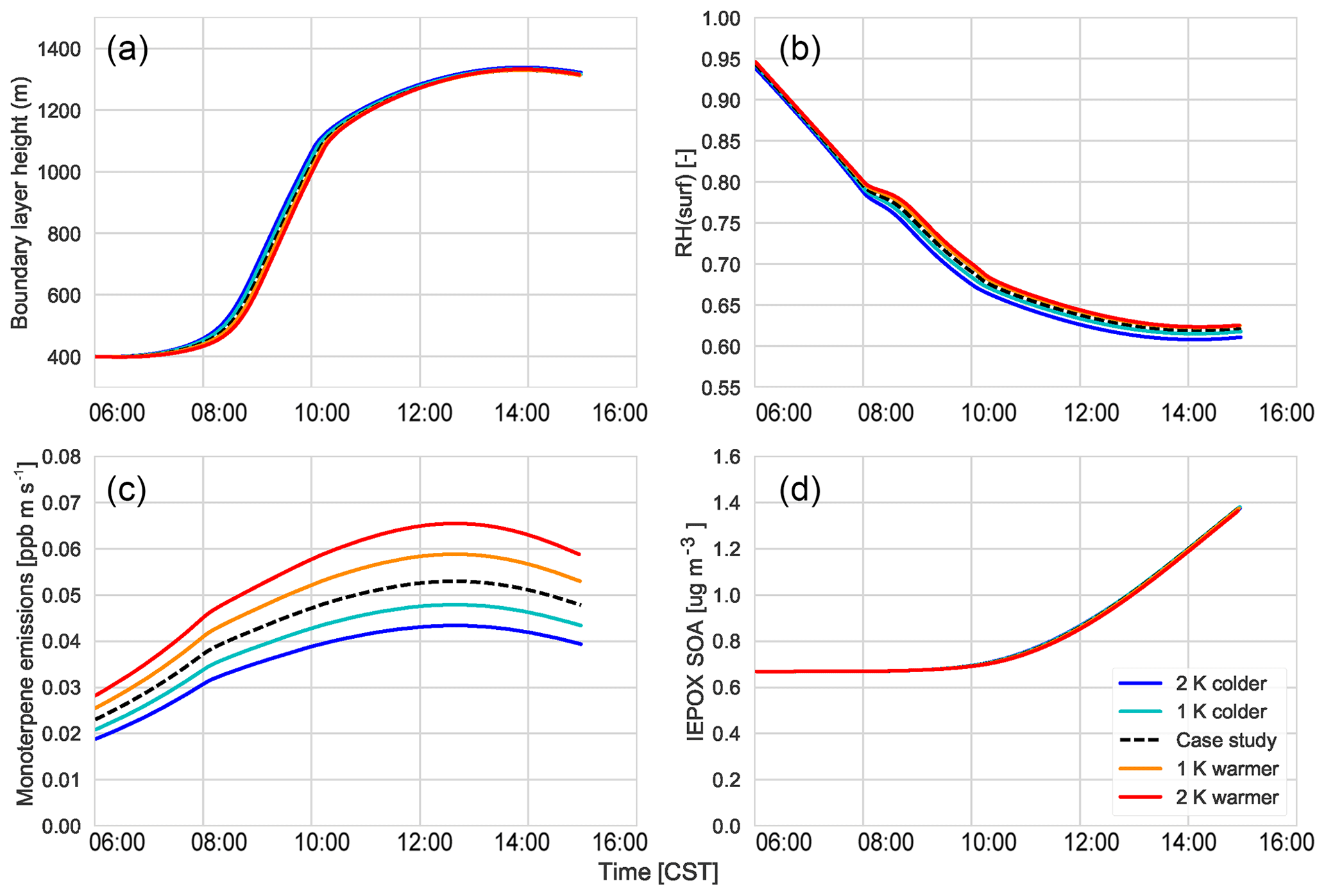
Figure C5Effect of temperature on boundary layer height (a), relative humidity (b), monoterpene emissions (c), and IEPOX SOA (d).

JN, RHHJ, JLF, MK, JLJ, and JVGdA were active in the conceptualization of the study and designed the methodology. JN performed the model simulations, carried out data analysis, and wrote the paper. RHHJ, JVGdA, MK, and JLF mentored JN. RHHJ developed the MXLCH-SOA code and JN carried out further code development. JLF, JLJ, and WH helped with the resources: they provided the data. All authors contributed to editing the paper.
The authors declare that they have no conflict of interest.
This paper has not been reviewed by the EPA and no endorsement should be inferred.
Weiwei Hu and Jose L. Jimenez acknowledge support from NOAA NA18OAR4310113
and EPA STAR 83587701-0.
Edited by: Manabu
Shiraiwa
Reviewed by: two anonymous referees
Ahmadov, R., McKeen, S., Robinson, A., Bahreini, R., Middlebrook, A., Gouw, J. D., Meagher, J., Hsie, E.-Y., Edgerton, E., Shaw, S., and Trainer, M.: A volatility basis set model for summertime secondary organic aerosols over the eastern United States in 2006, J. Geophys. Res.-Atmos., 117, D06301, https://doi.org/10.1029/2011JD016831, 2012. a
Atkinson, R. and Arey, J.: Atmospheric degradation of volatile organic compounds, Chem. Rev., 103, 4605–4638, 2003. a, b
Ayres, B. R., Allen, H. M., Draper, D. C., Brown, S. S., Wild, R. J., Jimenez, J. L., Day, D. A., Campuzano-Jost, P., Hu, W., de Gouw, J., Koss, A., Cohen, R. C., Duffey, K. C., Romer, P., Baumann, K., Edgerton, E., Takahama, S., Thornton, J. A., Lee, B. H., Lopez-Hilfiker, F. D., Mohr, C., Wennberg, P. O., Nguyen, T. B., Teng, A., Goldstein, A. H., Olson, K., and Fry, J. L.: Organic nitrate aerosol formation via NO3 + biogenic volatile organic compounds in the southeastern United States, Atmos. Chem. Phys., 15, 13377–13392, https://doi.org/10.5194/acp-15-13377-2015, 2015. a, b, c, d, e, f
Barbaro, E., de Arellano, J. V.-G., Ouwersloot, H. G., Schröter, J. S., Donovan, D. P., and Krol, M. C.: Aerosols in the convective boundary layer: Shortwave radiation effects on the coupled land-atmosphere system, J. Geophys. Res.-Atmos., 119, 5845–5863, https://doi.org/10.1002/2013JD021237, 2014. a, b
Betts, A. K.: Understanding hydrometeorology using global models, B. Am. Meteorol. Soc., 85, 1673–1688, 2004. a
Budisulistiorini, S. H., Li, X., Bairai, S. T., Renfro, J., Liu, Y., Liu, Y. J., McKinney, K. A., Martin, S. T., McNeill, V. F., Pye, H. O. T., Nenes, A., Neff, M. E., Stone, E. A., Mueller, S., Knote, C., Shaw, S. L., Zhang, Z., Gold, A., and Surratt, J. D.: Examining the effects of anthropogenic emissions on isoprene-derived secondary organic aerosol formation during the 2013 Southern Oxidant and Aerosol Study (SOAS) at the Look Rock, Tennessee ground site, Atmos. Chem. Phys., 15, 8871–8888, https://doi.org/10.5194/acp-15-8871-2015, 2015. a
Canagaratna, M., Jayne, J., Jimenez, J., Allan, J., Alfarra, M., Zhang, Q., Onasch, T., Drewnick, F., Coe, H., Middlebrook, A., Delia, A., Williams, L. R., Trimborn, A. M., Northway, M. J., DeCarlo, P. F., Kolb, C. E., Davidovits, P., and Worsnop, D. R.: Chemical and microphysical characterization of ambient aerosols with the aerodyne aerosol mass spectrometer, Mass Spectrom. Rev., 26, 185–222, 2007. a
Carlton, A. G., de Gouw, J., Jimenez, J. L., Ambrose, J. L., Attwood, A. R., Brown, S., Baker, K. R., Brock, C., Cohen, R. C., Edgerton, S., Farkas, C. M., Farmer, D., Goldstein, A. H., Gratz, L., Guenther, A., Hunt, S., Jaeglé, L., Jaffe, D. A., Mak, J., McClure, C., Nenes, A., Nguyen, T. K., Pierce, J. R., de Sa, S., Selin, N. E., Shah, V., Shaw, S., Shepson, P. B., Song, S., Stutz, J., Surratt, J. D., Turpin, B. J., Warneke, C., Washenfelder, R. A., Wennberg, P. O., and Zhou, X.: Synthesis of the Southeast Atmosphere Studies: Investigating Fundamental Atmospheric Chemistry Questions, B. Am. Meteorol. Soc., 99, 547–567, 2018. a
Crounse, J. D., Paulot, F., Kjaergaard, H. G., and Wennberg, P. O.: Peroxy radical isomerization in the oxidation of isoprene, Phys. Chem. Chem. Phys., 13, 13607–13613, https://doi.org/10.1039/c1cp21330j, 2011. a, b, c
DeCarlo, P. F., Kimmel, J. R., Trimborn, A., Northway, M. J., Jayne, J. T., Aiken, A. C., Gonin, M., Fuhrer, K., Horvath, T., Docherty, K. S., Worsnop, D. R., and Jimenez, J. L.: Field-deployable, high-resolution, time-of-flight aerosol mass spectrometer, Anal. Chem., 78, 8281–8289, 2006. a
Donahue, N., Robinson, A., Stanier, C., and Pandis, S.: Coupled partitioning, dilution, and chemical aging of semivolatile organics, Environ. Sci. Technol., 40, 2635–2643, 2006. a, b, c
Ehn, M., Thornton, J. A., Kleist, E., Sipilä, M., Junninen, H., Pullinen, I., Springer, M., Rubach, F., Tillmann, R., Lee, B., Lopez-Hilfiker, F., Andres, S., Acir, I.-H., Rissanen, M., Jokinen, T., Schobesberger, S., Kangasluoma, J., Kontkanen, J., Nieminen, T., Kurtén, T., Nielsen, L. B., Jørgensen, S., Kjaergaard, H. G., Canagaratna, M., Dal Maso, M., Berndt, T., Petäjä, T., Wahner, A., Kerminen, V.-M., Kulmala, M., Worsnop, D. R., Wildt, J., and Mentel, T. F.: A large source of low-volatility secondary organic aerosol, Nature, 506, 476, 2014. a
Emmerson, K. M., Cope, M. E., Galbally, I. E., Lee, S., and Nelson, P. F.: Isoprene and monoterpene emissions in south-east Australia: comparison of a multi-layer canopy model with MEGAN and with atmospheric observations, Atmos. Chem. Phys., 18, 7539–7556, https://doi.org/10.5194/acp-18-7539-2018, 2018. a
Farmer, D. K., Chen, Q., Kimmel, J. R., Docherty, K. S., Nemitz, E., Artaxo, P. a., Cappa, C. D., Martin, S. T., and Jimenez, J. L.: Chemically Resolved Particle Fluxes Over Tropical and Temperate Forests, Aerosol Sci. Tech., 47, 818–830, https://doi.org/10.1080/02786826.2013.791022, 2013. a
Field, R., Fritschen, L., Kanemasu, E., Smith, E., Stewart, J., Verma, S., and Kustas, W.: Calibration, comparison, and correction of net radiation instruments used during FIFE, J. Geophys. Res.-Atmos., 97, 18681–18695, 1992. a
Fisher, J. A., Jacob, D. J., Travis, K. R., Kim, P. S., Marais, E. A., Chan Miller, C., Yu, K., Zhu, L., Yantosca, R. M., Sulprizio, M. P., Mao, J., Wennberg, P. O., Crounse, J. D., Teng, A. P., Nguyen, T. B., St. Clair, J. M., Cohen, R. C., Romer, P., Nault, B. A., Wooldridge, P. J., Jimenez, J. L., Campuzano-Jost, P., Day, D. A., Hu, W., Shepson, P. B., Xiong, F., Blake, D. R., Goldstein, A. H., Misztal, P. K., Hanisco, T. F., Wolfe, G. M., Ryerson, T. B., Wisthaler, A., and Mikoviny, T.: Organic nitrate chemistry and its implications for nitrogen budgets in an isoprene- and monoterpene-rich atmosphere: constraints from aircraft (SEAC4RS) and ground-based (SOAS) observations in the Southeast US, Atmos. Chem. Phys., 16, 5969–5991, https://doi.org/10.5194/acp-16-5969-2016, 2016. a
Gaston, C. J., Riedel, T. P., Zhang, Z., Gold, A., Surratt, J. D., and Thornton, J. A.: Reactive uptake of an isoprene-derived epoxydiol to submicron aerosol particles, Environ. Sci. Technol., 48, 11178–11186, https://doi.org/10.1021/es5034266, 2014. a, b, c, d, e
Geron, C., Rasmussen, R., Arnts, R. R., and Guenther, A.: A review and synthesis of monoterpene speciation from forests in the United States, Atmos. Environ., 34, 1761–1781, 2000. a, b
Goldstein, A. H., Koven, C. D., Heald, C. L., and Fung, I. Y.: Biogenic carbon and anthropogenic pollutants combine to form a cooling haze over the southeastern United States, P. Natl. Acad. Sci. USA, 106, 8835–8840, 2009. a, b, c, d, e
Guenther, A., Hewitt, C. N., Erickson, D., Fall, R., Geron, C., Graedel, T., Harley, P., Klinger, L., Lerdau, M., McKay, W., Pierce, T., Scholes, B., Steinbrecher, R., Tallamraju, R., Taylor, J., and Zimmerman, P.: A global model of natural volatile organic compound emissions, J. Geophys. Res.-Atmos., 100, 8873–8892, 1995. a, b
Guenther, A., Karl, T., Harley, P., Wiedinmyer, C., Palmer, P. I., and Geron, C.: Estimates of global terrestrial isoprene emissions using MEGAN (Model of Emissions of Gases and Aerosols from Nature), Atmos. Chem. Phys., 6, 3181–3210, https://doi.org/10.5194/acp-6-3181-2006, 2006. a, b, c, d, e, f, g, h, i, j, k, l, m
Guenther, A., Jiang, X., Heald, C., Sakulyanontvittaya, T., Duhl, T., Emmons, L., and Wang, X.: The Model of Emissions of Gases and Aerosols from Nature version 2.1 (MEGAN2. 1): an extended and updated framework for modeling biogenic emissions, 2012. a
Hansen, J., Ruedy, R., Glascoe, J., and Sato, M.: GISS analysis of surface temperature change, J. Geophys. Res.-Atmos., 104, 30997–31022, 1999. a
Hansen, J., Ruedy, R., Sato, M., Imhoff, M., Lawrence, W., Easterling, D., Peterson, T., and Karl, T.: A closer look at United States and global surface temperature change, J. Geophys. Res.-Atmos., 106, 23947–23963, 2001. a
Hidy, G. M., Blanchard, C. L., Baumann, K., Edgerton, E., Tanenbaum, S., Shaw, S., Knipping, E., Tombach, I., Jansen, J., and Walters, J.: Chemical climatology of the southeastern United States, 1999–2013, Atmos. Chem. Phys., 14, 11893–11914, https://doi.org/10.5194/acp-14-11893-2014, 2014. a
Holzinger, R., Lee, A., Paw, K. T., and Goldstein, U. A. H.: Observations of oxidation products above a forest imply biogenic emissions of very reactive compounds, Atmos. Chem. Phys., 5, 67–75, https://doi.org/10.5194/acp-5-67-2005, 2005. a, b, c
Horowitz, L. W., Fiore, A. M., Milly, G. P., Cohen, R. C., Perring, A., Wooldridge, P. J., Hess, P. G., Emmons, L. K., and Lamarque, J.-F.: Observational constraints on the chemistry of isoprene nitrates over the eastern United States, J. Geophys. Res.-Atmos., 112, 2007. a
Hu, W., Palm, B. B., Day, D. A., Campuzano-Jost, P., Krechmer, J. E., Peng, Z., de Sá, S. S., Martin, S. T., Alexander, M. L., Baumann, K., Hacker, L., Kiendler-Scharr, A., Koss, A. R., de Gouw, J. A., Goldstein, A. H., Seco, R., Sjostedt, S. J., Park, J.-H., Guenther, A. B., Kim, S., Canonaco, F., Prévôt, A. S. H., Brune, W. H., and Jimenez, J. L.: Volatility and lifetime against OH heterogeneous reaction of ambient isoprene-epoxydiols-derived secondary organic aerosol (IEPOX-SOA), Atmos. Chem. Phys., 16, 11563–11580, https://doi.org/10.5194/acp-16-11563-2016, 2016. a, b, c, d, e, f, g, h, i, j, k, l, m, n, o, p, q, r
Hu, W. W., Campuzano-Jost, P., Palm, B. B., Day, D. A., Ortega, A. M., Hayes, P. L., Krechmer, J. E., Chen, Q., Kuwata, M., Liu, Y. J., de Sá, S. S., McKinney, K., Martin, S. T., Hu, M., Budisulistiorini, S. H., Riva, M., Surratt, J. D., St. Clair, J. M., Isaacman-Van Wertz, G., Yee, L. D., Goldstein, A. H., Carbone, S., Brito, J., Artaxo, P., de Gouw, J. A., Koss, A., Wisthaler, A., Mikoviny, T., Karl, T., Kaser, L., Jud, W., Hansel, A., Docherty, K. S., Alexander, M. L., Robinson, N. H., Coe, H., Allan, J. D., Canagaratna, M. R., Paulot, F., and Jimenez, J. L.: Characterization of a real-time tracer for isoprene epoxydiols-derived secondary organic aerosol (IEPOX-SOA) from aerosol mass spectrometer measurements, Atmos. Chem. Phys., 15, 11807–11833, https://doi.org/10.5194/acp-15-11807-2015, 2015. a, b, c, d, e, f, g
Janssen, R. H. H., Vilà-Guerau de Arellano, J., Ganzeveld, L. N., Kabat, P., Jimenez, J. L., Farmer, D. K., van Heerwaarden, C. C., and Mammarella, I.: Combined effects of surface conditions, boundary layer dynamics and chemistry on diurnal SOA evolution, Atmos. Chem. Phys., 12, 6827–6843, https://doi.org/10.5194/acp-12-6827-2012, 2012. a, b, c, d, e, f
Janssen, R., Vilà-Guerau de Arellano, J., Jimenez, J., Ganzeveld, L., Robinson, N., Allan, J., Coe, H., and Pugh, T.: Influence of boundary layer dynamics and isoprene chemistry on the organic aerosol budget in a tropical forest, J. Geophys. Res.-Atmos., 118, 9351–9366, 2013. a, b, c, d
Janssen, R., Tsimpidi, A., Karydis, V., Pozzer, A., Lelieveld, J., Crippa, M., Prévôt, A., Ait-Helal, W., Borbon, A., Sauvage, S., and Locoge, N.: Influence of local production and vertical transport on the organic aerosol budget over Paris, J. Geophys. Res.-Atmos., 122, 8276–8296, 2017. a
Jimenez, J., Canagaratna, M., Donahue, N., Prevot, A., Zhang, Q., Kroll, J. H., DeCarlo, P. F., Allan, J. D., Coe, H., Ng, N. L., Aiken, A. C., Docherty, K. S., Ulbrich, I. M., Grieshop, A. P., Robinson, A. L., Duplissy, J., Smith, J. D., Wilson, K. R., Lanz, V. A., Hueglin, C., Sun, Y. L., Tian, J., Laaksonen, A., Raatikaine, T., Rautiainen, J., Vaattovaara, P., Ehn, M., Kulmala, M., Tomlinson, J. M., Collins, D. R., Cubison, M. J., Dunlea, E. J., Huffman, J. A., Onasch, T. B., Alfarra, M. R., Williams, P. I., Bower, K., Kondo, Y., Schneider, J., Drewnick, F., Borrmann, S., Weimer, S., Demerjian, K., Salcedo, D., Cottrell, L., Griffin, R., Takami, A., Miyoshi, T., Hatakeyama, S., Shimono, A., Sun, J. Y., Zhang, Y. M., Dzepina, K., Kimmel, J. R., Sueper, D., Jayne, J. T., Herndon, S. C., Trimborn, A. M., Williams, L. R., Wood, E. C., Middlebrook, A. M., Kolb, C. E., Baltensperger, U. and Worsnop, D. R.: Evolution of organic aerosols in the atmosphere, Science, 326, 1525–1529, 2009. a, b
Karl, T., Guenther, A., Yokelson, R. J., Greenberg, J., Potosnak, M., Blake, D. R., and Artaxo, P.: The tropical forest and fire emissions experiment: Emission, chemistry, and transport of biogenic volatile organic compounds in the lower atmosphere over Amazonia, J. Geophys. Res.-Atmos., 112, D18302, https://doi.org/10.1029/2007JD008539, 2007. a
Karl, T., Guenther, A., Turnipseed, A., Tyndall, G., Artaxo, P., and Martin, S.: Rapid formation of isoprene photo-oxidation products observed in Amazonia, Atmos. Chem. Phys., 9, 7753–7767, https://doi.org/10.5194/acp-9-7753-2009, 2009. a
Karl, T., Harley, P., Emmons, L., Thornton, B., Guenther, A., Basu, C., Turnipseed, A., and Jardine, K.: Efficient Atmospheric Cleansing of Oxidized Organic Trace Gases by Vegetation, Science, 330, 816–819, https://doi.org/10.1126/science.1192534, 2010. a
Kim, P. S., Jacob, D. J., Fisher, J. A., Travis, K., Yu, K., Zhu, L., Yantosca, R. M., Sulprizio, M. P., Jimenez, J. L., Campuzano-Jost, P., Froyd, K. D., Liao, J., Hair, J. W., Fenn, M. A., Butler, C. F., Wagner, N. L., Gordon, T. D., Welti, A., Wennberg, P. O., Crounse, J. D., St. Clair, J. M., Teng, A. P., Millet, D. B., Schwarz, J. P., Markovic, M. Z., and Perring, A. E.: Sources, seasonality, and trends of southeast US aerosol: an integrated analysis of surface, aircraft, and satellite observations with the GEOS-Chem chemical transport model, Atmos. Chem. Phys., 15, 10411–10433, https://doi.org/10.5194/acp-15-10411-2015, 2015. a, b
Kjaergaard, H. G., Knap, H. C., Ørnsø, K. B., Jørgensen, S., Crounse, J. D., Paulot, F., and Wennberg, P. O.: Atmospheric fate of methacrolein. 2. Formation of lactone and implications for organic aerosol production, J. Phys. Chem. A, 116, 5763–5768, 2012. a
Krechmer, J. E., Coggon, M. M., Massoli, P., Nguyen, T. B., Crounse, J. D., Hu, W., Day, D. A., Tyndall, G. S., Henze, D. K., Rivera-Rios, J. C., Nowak, J. B., Kimmel, J. R., Mauldin, R. L., Stark, H., Jayne, J. T., Sipilä, M., Junninen, H., St. Clair, J. M., Zhang, X., Feiner, P. A., Zhang, L., Miller, D. O., Brune, W. H., Keutsch, F. N., Wennberg, P. O., Seinfeld, J. H., Worsnop, D. R., Jimenez, J. L., and Canagaratna, M. R.: Formation of Low Volatility Organic Compounds and Secondary Organic Aerosol from Isoprene Hydroxyhydroperoxide Low-NO Oxidation, Environ. Sci. Technol., 49, 10330–10339, https://doi.org/10.1021/acs.est.5b02031, 2015. a, b, c, d, e, f, g, h, i, j, k, l, m, n, o
Lee, A., Goldstein, A. H., Kroll, J. H., Ng, N. L., Varutbangkul, V., Flagan, R. C., and Seinfeld, J. H.: Gas-phase products and secondary aerosol yields from the photooxidation of 16 different terpenes, J. Geophys. Res.-Atmos., 111, D17305, https://doi.org/10.1029/2006JD007050, 2006. a
Liao, H., Henze, D. K., Seinfeld, J. H., Wu, S., and Mickley, L. J.: Biogenic secondary organic aerosol over the United States: Comparison of climatological simulations with observations, J. Geophys. Res.-Atmos., 112, D06201, https://doi.org/10.1029/2006JD007813, 2007. a
Lilly, D. K.: Models of cloud-topped mixed layers under a strong inversion, Q. J. Roy. Meteor. Soc., 94, 292–309, 1968. a
Liu, J., D'Ambro, E. L., Lee, B. H., Lopez-Hilfiker, F. D., Zaveri, R. A., Rivera-Rios, J. C., Keutsch, F. N., Iyer, S., Kurten, T., Zhang, Z., Gold, A., Surratt, J. D., Shilling, J. E., and Thornton, J. A.: Efficient isoprene secondary organic aerosol formation from a non-IEPOX pathway, Environ. Sci. Technol., 50, 9872–9880, 2016. a
Lopez-Hilfiker, F., Mohr, C., D'Ambro, E. L., Lutz, A., Riedel, T. P., Gaston, C. J., Iyer, S., Zhang, Z., Gold, A., Surratt, J. D., Lee, B. H., Kurten, T., Hu, W. W., Jimenez, J., Hallquist, M., and Thornton, J. A.: Molecular composition and volatility of organic aerosol in the Southeastern US: implications for IEPOX derived SOA, Environ. Sci. Technol., 50, 2200–2209, 2016a. a
Lopez-Hilfiker, F. D., Mohr, C., D'Ambro, E. L., Lutz, A., Riedel, T. P., Gaston, C. J., Iyer, S., Zhang, Z., Gold, A., Surratt, J. D., Lee, B. H., Kurten, T., Hu, W. W., Jimenez, J., Hallquist, M., and Thornton, J. A.: Molecular Composition and Volatility of Organic Aerosol in the Southeastern U.S.: Implications for IEPOX Derived SOA, Environ. Sci. Technol., 50, 2200–2209, https://doi.org/10.1021/acs.est.5b04769, 2016b. a
Marais, E. A., Jacob, D. J., Jimenez, J. L., Campuzano-Jost, P., Day, D. A., Hu, W., Krechmer, J., Zhu, L., Kim, P. S., Miller, C. C., Fisher, J. A., Travis, K., Yu, K., Hanisco, T. F., Wolfe, G. M., Arkinson, H. L., Pye, H. O. T., Froyd, K. D., Liao, J., and McNeill, V. F.: Aqueous-phase mechanism for secondary organic aerosol formation from isoprene: application to the southeast United States and co-benefit of SO2 emission controls, Atmos. Chem. Phys., 16, 1603–1618, https://doi.org/10.5194/acp-16-1603-2016, 2016. a, b, c, d
Mauderly, J. L. and Chow, J. C.: Health effects of organic aerosols, Inhal. Toxicol., 20, 257–288, 2008. a
Monteith, J. L.: Evaporation and environment, Symp. Soc. Exp. Biol., 19, 205–234, 1965. a
Nguyen, T. B., Bates, K. H., Crounse, J. D., Schwantes, R. H., Zhang, X., Kjaergaard, H. G., Surratt, J. D., Lin, P., Laskin, A., Seinfeld, J. H., and Wennberg, P. O.: Mechanism of the hydroxyl radical oxidation of methacryloyl peroxynitrate (MPAN) and its pathway toward secondary organic aerosol formation in the atmosphere, Phys. Chem. Chem. Phys., 17, 17914–17926, https://doi.org/10.1039/C5CP02001H, 2015a. a, b
Nguyen, T. B., Crounse, J. D., Teng, A. P., Clair, J. M. S., Paulot, F., Wolfe, G. M., and Wennberg, P. O.: Rapid deposition of oxidized biogenic compounds to a temperate forest, P. Natl. Acad. Sci. USA, 112, E392–E401, 2015b. a
Orlando, J. J. and Tyndall, G. S.: Laboratory studies of organic peroxy radical chemistry: an overview with emphasis on recent issues of atmospheric significance, Chem. Soc. Rev., 41, 6294, https://doi.org/10.1039/c2cs35166h, 2012. a, b
Ouwersloot, H. G., Vilà-Guerau de Arellano, J., van Heerwaarden, C. C., Ganzeveld, L. N., Krol, M. C., and Lelieveld, J.: On the segregation of chemical species in a clear boundary layer over heterogeneous land surfaces, Atmos. Chem. Phys., 11, 10681–10704, https://doi.org/10.5194/acp-11-10681-2011, 2011. a
Pan, Z., Liu, X., Kumar, S., Gao, Z., and Kinter, J.: Intermodel variability and mechanism attribution of central and southeastern US anomalous cooling in the twentieth century as simulated by CMIP5 models, J. Climate, 26, 6215–6237, 2013. a
Paulot, F., Crounse, J. D., Kjaergaard, H. G., Kürten, A., Clair, J. M. S., Seinfeld, J. H., and Wennberg, P. O.: Unexpected epoxide formation in the gas-phase photooxidation of isoprene, Science, 325, 730–733, 2009. a, b
Pratt, K. A., Mielke, L. H., Shepson, P. B., Bryan, A. M., Steiner, A. L., Ortega, J., Daly, R., Helmig, D., Vogel, C. S., Griffith, S., Dusanter, S., Stevens, P. S., and Alaghmand, M.: Contributions of individual reactive biogenic volatile organic compounds to organic nitrates above a mixed forest, Atmos. Chem. Phys., 12, 10125–10143, https://doi.org/10.5194/acp-12-10125-2012, 2012. a
Pye, H. O. T., Chan, A. W. H., Barkley, M. P., and Seinfeld, J. H.: Global modeling of organic aerosol: the importance of reactive nitrogen (NOx and NO3), Atmos. Chem. Phys., 10, 11261–11276, https://doi.org/10.5194/acp-10-11261-2010, 2010. a, b, c, d, e, f
Pye, H. O. T., Pinder, R. W., Piletic, I. R., Xie, Y., Capps, S. L., Lin, Y. H., Surratt, J. D., Zhang, Z., Gold, A., Luecken, D. J., Hutzell, W. T., Jaoui, M., Offenberg, J. H., Kleindienst, T. E., Lewandowski, M., and Edney, E. O.: Epoxide pathways improve model predictions of isoprene markers and reveal key role of acidity in aerosol formation, Environ. Sci. Technol., 47, 11056–11064, https://doi.org/10.1021/es402106h, 2013. a
Sakulyanontvittaya, T., Duhl, T., Wiedinmyer, C., Helmig, D., Matsunaga, S., Potosnak, M., Milford, J., and Guenther, A.: Monoterpene and sesquiterpene emission estimates for the United States, Environ. Sci. Technol., 42, 1623–1629, 2008. a
Saunders, S. M., Jenkin, M. E., Derwent, R. G., and Pilling, M. J.: Protocol for the development of the Master Chemical Mechanism, MCM v3 (Part A): tropospheric degradation of non-aromatic volatile organic compounds, Atmos. Chem. Phys., 3, 161–180, https://doi.org/10.5194/acp-3-161-2003, 2003. a
Spracklen, D. V., Jimenez, J. L., Carslaw, K. S., Worsnop, D. R., Evans, M. J., Mann, G. W., Zhang, Q., Canagaratna, M. R., Allan, J., Coe, H., McFiggans, G., Rap, A., and Forster, P.: Aerosol mass spectrometer constraint on the global secondary organic aerosol budget, Atmos. Chem. Phys., 11, 12109–12136, https://doi.org/10.5194/acp-11-12109-2011, 2011. a
Stark, H., Yatavelli, R. L., Thompson, S. L., Kang, H., Krechmer, J. E., Kimmel, J. R., Palm, B. B., Hu, W., Hayes, P. L., Day, D. A., Campuzano-Jost, P., Canagaratna, M. R., Jayne, J. T., Worsnop, D. R., and Jimenez, J. L.: Impact of thermal decomposition on thermal desorption instruments: advantage of thermogram analysis for quantifying volatility distributions of organic species, Environ. Sci. Technol., 51, 8491–8500, 2017. a
Stull, R.: An Introduction to Boundary Layer Meteorology, Kluwer Academic Publishers, Dordrecht 1988. a
Su, L., Patton, E. G., Vilà-Guerau de Arellano, J., Guenther, A. B., Kaser, L., Yuan, B., Xiong, F., Shepson, P. B., Zhang, L., Miller, D. O., Brune, W. H., Baumann, K., Edgerton, E., Weinheimer, A., Misztal, P. K., Park, J.-H., Goldstein, A. H., Skog, K. M., Keutsch, F. N., and Mak, J. E.: Understanding isoprene photooxidation using observations and modeling over a subtropical forest in the southeastern US, Atmos. Chem. Phys., 16, 7725–7741, https://doi.org/10.5194/acp-16-7725-2016, 2016. a, b, c, d, e, f, g, h, i, j, k, l, m, n, o, p, q
Takekawa, H., Minoura, H., and Yamazaki, S.: Temperature dependence of secondary organic aerosol formation by photo-oxidation of hydrocarbons, Atmos. Environ., 37, 3413–3424, 2003. a
Tennekes, H.: A model for the dynamics of the inversion above a convective boundary layer, J. Atmos. Sci., 30, 558–567, 1973. a, b
Tennekes, H. and Driedonks, A.: Basic entrainment equations for the atmospheric boundary layer, Bound.-Lay. Meteorol., 20, 515–531, 1981. a
Ulbrich, I. M., Canagaratna, M. R., Zhang, Q., Worsnop, D. R., and Jimenez, J. L.: Interpretation of organic components from Positive Matrix Factorization of aerosol mass spectrometric data, Atmos. Chem. Phys., 9, 2891–2918, https://doi.org/10.5194/acp-9-2891-2009, 2009. a
Van Heerwaarden, C. C., Vilà-Guerau de Arellano, J., Moene, A. F., and Holtslag, A. A.: Interactions between dry-air entrainment, surface evaporation and convective boundary-layer development, Q. J. Roy. Meteor. Soc., 135, 1277–1291, 2009. a, b, c, d, e, f
Vilà-Guerau de Arellano, J., van den Dries, K., and Pino, D.: On inferring isoprene emission surface flux from atmospheric boundary layer concentration measurements, Atmos. Chem. Phys., 9, 3629–3640, https://doi.org/10.5194/acp-9-3629-2009, 2009. a
Vilà-Guerau de Arellano, J., van Heerwaarden, C. C., van Stratum, B. J., and van den Dries, K.: Atmospheric boundary layer: Integrating air chemistry and land interactions, Cambridge University Press, 2015. a, b, c
Wagner, N. L., Brock, C. A., Angevine, W. M., Beyersdorf, A., Campuzano-Jost, P., Day, D., de Gouw, J. A., Diskin, G. S., Gordon, T. D., Graus, M. G., Holloway, J. S., Huey, G., Jimenez, J. L., Lack, D. A., Liao, J., Liu, X., Markovic, M. Z., Middlebrook, A. M., Mikoviny, T., Peischl, J., Perring, A. E., Richardson, M. S., Ryerson, T. B., Schwarz, J. P., Warneke, C., Welti, A., Wisthaler, A., Ziemba, L. D., and Murphy, D. M.: In situ vertical profiles of aerosol extinction, mass, and composition over the southeast United States during SENEX and SEAC4RS: observations of a modest aerosol enhancement aloft, Atmos. Chem. Phys., 15, 7085–7102, https://doi.org/10.5194/acp-15-7085-2015, 2015. a, b
Wang, P., Schade, G., Estes, M., and Ying, Q.: Improved MEGAN predictions of biogenic isoprene in the contiguous United States, Atmos. Environ., 148, 337–351, 2017. a
Warneke, C., Trainer, M., de Gouw, J. A., Parrish, D. D., Fahey, D. W., Ravishankara, A. R., Middlebrook, A. M., Brock, C. A., Roberts, J. M., Brown, S. S., Neuman, J. A., Lerner, B. M., Lack, D., Law, D., Hübler, G., Pollack, I., Sjostedt, S., Ryerson, T. B., Gilman, J. B., Liao, J., Holloway, J., Peischl, J., Nowak, J. B., Aikin, K. C., Min, K.-E., Washenfelder, R. A., Graus, M. G., Richardson, M., Markovic, M. Z., Wagner, N. L., Welti, A., Veres, P. R., Edwards, P., Schwarz, J. P., Gordon, T., Dube, W. P., McKeen, S. A., Brioude, J., Ahmadov, R., Bougiatioti, A., Lin, J. J., Nenes, A., Wolfe, G. M., Hanisco, T. F., Lee, B. H., Lopez-Hilfiker, F. D., Thornton, J. A., Keutsch, F. N., Kaiser, J., Mao, J., and Hatch, C. D.: Instrumentation and measurement strategy for the NOAA SENEX aircraft campaign as part of the Southeast Atmosphere Study 2013, Atmos. Meas. Tech., 9, 3063–3093, https://doi.org/10.5194/amt-9-3063-2016, 2016. a, b, c, d
Weaver, H. L.: Temperature and humidity flux-variance relations determined by one-dimensional eddy correlation, Bound.-Lay. Meteorol., 53, 77–91, 1990. a
Wennberg, P. O., Bates, K. H., Crounse, J. D., Dodson, L. G., McVay, R. C., Mertens, L. A., Nguyen, T. B., Praske, E., Schwantes, R. H., Smarte, M. D., Clair, J. M. St, Teng, A. P., Zhang, X., and Seinfeld, J. H.: Gas-phase reactions of isoprene and its major oxidation products, Chem. Rev., 118, 3337–3390, 2018. a
Xu, L., Guo, H., Boyd, C. M., Klein, M., Bougiatioti, A., Cerully, K. M., Hite, J. R., Isaacman-VanWertz, G., Kreisberg, N. M., Knote, C., Olson, K., Koss, A., Goldstein, A. H., Hering, S. V., de Gouw, J., Baumann, K., Lee, S.-H., Nenes, A., Weber, R. J., and Lee Ng, N.: Effects of anthropogenic emissions on aerosol formation from isoprene and monoterpenes in the southeastern United States, P. Natl. Acad. Sci. USA, 112, 37–42, 2015. a, b, c, d, e, f, g
Xu, L., Pye, H. O. T., He, J., Chen, Y., Murphy, B. N., and Ng, N. L.: Experimental and model estimates of the contributions from biogenic monoterpenes and sesquiterpenes to secondary organic aerosol in the southeastern United States, Atmos. Chem. Phys., 18, 12613–12637, https://doi.org/10.5194/acp-18-12613-2018, 2018. a
Zhang, H., Yee, L. D., Lee, B. H., Curtis, M. P., Worton, D. R., Isaacman-VanWertz, G., Offenberg, J. H., Lewandowski, M., Kleindienst, T. E., Beaver, M. R., Holder, A. L., Lonneman, W. A., Docherty, K. S., Jaoui, M., Pye, H. O. T., Hu, W., Day, D. A., Campuzano-Jost, P., Jimenez, J. L., Guo, H., Weber, R. J., de Gouw, J., Koss, A. R., Edgerton, E. S., Brune, W., Mohr, C., Lopez-Hilfiker, F. D., Lutz, A., Kreisberg, N. M., Spielman, S. R., Hering, S. V., Wilson, K. R., Thornton, J. A., and Goldstein, A. H.: Monoterpenes are the largest source of summertime organic aerosol in the southeastern United States, P. Natl. Acad. Sci. USA, 115, 2038–2043, 2018. a, b, c
Zhang, Q., Jimenez, J. L., Canagaratna, M., Allan, J., Coe, H., Ulbrich, I., Alfarra, M., Takami, A., Middlebrook, A., Sun, Y. L., Dzepina, K., and Dunlea, E.: Ubiquity and dominance of oxygenated species in organic aerosols in anthropogenically-influenced Northern Hemisphere midlatitudes, Geophys. Res. Lett., 34, L13801, https://doi.org/10.1029/2007GL029979, 2007. a
- Abstract
- Introduction
- Site and data description
- Model description
- Numerical experiments
- Results
- Budget analysis
- Sensitivity analysis: early morning SOA profile
- Sensitivity analysis: SOA formation in a changing climate
- Conclusion
- Code and data availability
- Appendix A: Model initialisation
- Appendix B: Interactive isoprene and monoterpene emissions calculations
- Appendix C: Supporting figures
- Author contributions
- Competing interests
- Disclaimer
- Acknowledgements
- References