Variability of temperature and ozone in the upper troposphere and lower stratosphere from multi-satellite observations and reanalysis data

Temperature and ozone changes in the upper troposphere and lower stratosphere (UTLS) are important components of climate change. In this paper, variability and trends of temperature and ozone in the UTLS are investigated for the period 2002–2017 using high-quality, high vertical resolution Global Navigation Satellite System radio occultation (GNSS RO) data and improved merged satellite data sets. As part of the Stratosphere-troposphere Processes And their Role in Climate (SPARC) Reanalysis Intercomparison Project (S-RIP), three reanalysis data sets, including the ERA-I, MERRA2 and the recently released ERA5, are evaluated for their representation of temperature and ozone in the UTLS. The recent temperature and ozone trends are updated with a multiple linear regression (MLR) method and related to sea surface temperature (SST) changes based on model simulations made with NCAR's Whole Atmosphere Community Climate Model (WACCM).

All reanalysis temperatures show good agreement with the GNSS RO measurements in both absolute value and annual cycle. Interannual variations in temperature related to Quasi-Biennial Oscillation (QBO) and the El Niño–Southern Oscillation (ENSO) processes are well represented by all reanalyses. However, evident biases can be seen in reanalyses for the linear trends of temperature since they are affected by discontinuities in assimilated observations and methods. Such biases can be corrected and the estimated trends can be significantly improved. ERA5 is significantly improved compared to ERA-I and shows the best agreement with the GNSS RO temperature.

The MLR results indicate a significant warming of 0.2–0.3 K per decade in most areas of the troposphere, with a stronger increase of 0.4–0.5 K per decade at midlatitudes of both hemispheres. In contrast, the stratospheric temperature decreases at a rate of 0.1–0.3 K per decade, which is most significant in the Southern Hemisphere (SH). Positive temperature trends of 0.1–0.3 K per decade are seen in the tropical lower stratosphere (100–50 hPa). Negative trends of ozone are found in the Northern Hemisphere (NH) at 150–50 hPa, while positive trends are evident in the tropical lower stratosphere. Asymmetric trends of ozone can be found in the midlatitudes of two hemispheres in the middle stratosphere, with significant ozone decrease in the NH and increase in ozone in the SH. Large biases exist in reanalyses, and it is still challenging to do trend analysis based on reanalysis ozone data.

According to single-factor-controlled model simulations with WACCM, the temperature increase in the troposphere and the ozone decrease in the NH stratosphere are mainly connected to the increase in SST and subsequent changes of atmospheric circulations. Both the increase in SSTs and the decrease in ozone in the NH contribute to the temperature decrease in the NH stratosphere. The increase in temperature in the lower stratospheric tropics may be related to an increase in ozone in that region, while warming SSTs contribute to a cooling in that area.

1 Introduction

The upper troposphere and lower stratosphere (UTLS) is a key region for stratosphere–troposphere coupling and affects the content of trace gases in both the troposphere and the stratosphere (Staten and Reichler, 2008; Fueglistaler et al., 2014). Temperature change in the UTLS is an important component of climate change and has been extensively studied (Randel et al., 2009; Wang et al., 2012; Kim et al., 2013; Wang et al., 2013). While measurements in the UTLS are relatively sparse, reanalysis data are widely used to investigate temperature variabilities (Xie et al., 2012; Wang et al., 2016). Atmospheric reanalysis data assimilate ground-based data, satellite-based data and other data sources to provide the current best estimation of the real atmosphere with global spatial and temporal coverage. However, because of the lack of high-quality and high vertical resolution temperature observations and also the low vertical resolution of the model, the reanalysis data in the UTLS might be problematic (Zhao and Li, 2006; Trenberth and Smith, 2006, 2009). It is useful, therefore, to quantify the accuracy and variability of reanalysis temperature fields.

A comprehensive assessment of the accuracy of the reanalysis temperature has been challenging because of the lack of high-quality observations with high temporal and high spatial resolution. For example, ground-based radiosonde measurements often have low temporal and spatial resolution (distributed mostly in the Northern Hemisphere), while nadir-sounding satellite measurements (e.g., the Microwave Sounding Unit) can not resolve the narrow vertical-scale features in the UTLS well. Global Navigation Satellite System radio occultation (GNSS RO) is a relatively new technology that measures the time delay in occulted signals from one satellite to another and provides information for deriving profiles of atmospheric temperature and moisture. Since the Challenging Minisatellite Payload (CHAMP) mission launched in 2001, GNSS RO has provided high-quality and high vertical resolution temperature measurements in the UTLS for almost 2 decades. Due to its self-calibrating and it not being susceptible to instrument drift (Anthes et al., 2008), GNSS RO provides a stable temperature record that is well suited to validating the reanalysis data.

Atmospheric reanalysis has been developed for decades. While more and more observations are available and more advanced techniques are used in the assimilation system, a new generation of reanalysis is expected to be significantly improved. The European Center for Medium-Range Weather Forecasts (ECMWF) released its fifth-generation reanalysis (ERA5) in 2017. It is very interesting to see how the quality of temperatures in the UTLS has been improved in ERA5. The primary goal of this study is to evaluate the UTLS temperature in the newest ERA5 reanalysis using the GNSS RO as a reference. Within the context of the Stratosphere-troposphere Processes And their Role in Climate (SPARC) Reanalysis Intercomparison Project (S-RIP), the Modern-Era Retrospective analysis for Research and Application version 2 (MERRA2) and the ERA-Interim (ERA-I) are also included for a comparison.

To give a comprehensive assessment of the reanalysis temperature in the UTLS, the interannual variations and the long-term trends of temperature are compared between the GNSS RO and different reanalysis data sets. Interannual variabilities of temperatures in the UTLS are related to complex processes, such as the Quasi-Biennial Oscillation (QBO) and the El Niño–Southern Oscillation (ENSO) (Xie et al., 2012; Randel and Wu, 2015; Garfinkel et al., 2018). QBO- and ENSO-related temperature signals in the UTLS are analyzed to evaluate the capability of reanalysis data to represent QBO- and ENSO-related signals well. While assimilating many types of observations, reanalysis data suffer from instrument exchanges and may exhibit sudden changes as new data are assimilated (Sturaro, 2003; Sterl, 2004). Such discontinuities may strongly influence the long-term trends calculated from reanalysis data. Finding out how well the reanalysis data can represent the interannual variability and the long-term trends of temperatures in the UTLS is the second goal of this study.

Long-term trends are a key issue in UTLS studies. A net cooling in the stratosphere was seen over the past decades (Randel et al., 2009; Flato et al., 2014). However, large discrepancies of the temperature trends in the UTLS have been reported between different observational and reanalysis data sets (Wang et al., 2012; Xie et al., 2012) and also between data and models (Kim et al., 2013). Recently, a slowing down of cooling in the lower stratosphere since 1998 (Polvani et al., 2017) or an increase in temperature in the tropical tropopause layer since 2001 (Wang et al., 2013) have been reported, which makes it more complicated to fully understand the UTLS temperature trend. Temperature changes in the UTLS are related to both internal processes, e.g., sea surface temperature (SST) variations and external forcing, such as greenhouse gases (GHGs) and ozone-depleting substances (ODSs) (Randel et al., 2009; Flato et al., 2014). If the slowing down or changing in sign of temperature in the UTLS will persist in the future is an open question. Whether the turning of temperature trends around 2000 is related to internal processes like SST variations (Wang et al., 2015, 2016) or caused by ozone changes (Polvani and Solomon, 2012; Polvani et al., 2017) is still not clear. The third goal of this study is to update the recent temperature trend in the UTLS using a combination of GNSS RO and reanalysis data sets and attribute it to different factors like SST and ozone changes.

To understand the relationship between ozone and temperature changes in the UTLS, the recent variability of ozone is also analyzed. Ozone is closely coupled to temperature changes in the UTLS. Abalos et al. (2012) studied the temporal variability of the upwelling near the tropopause using MLS (Microwave Limb Sounder) ozone (or CO) and ERA-I temperature or wind and demonstrated the high correlation between the upwelling, temperatures and tracers. Schoeberl et al. (2008) found that photochemical processes force fluctuations in the trace gases (such as ozone) to be synchronized with annual and QBO variations in the zonal mean residual vertical velocity. Changes in ozone concentrations may impact temperature directly through their radiative effects (Forster et al., 2007; Abalos et al., 2012; Maycock, 2016; Gilford et al., 2016) or indirectly through their modulation to atmospheric circulations (Polvani et al., 2017). The recent variability of ozone in the UTLS has been investigated by several studies. Harris et al. (2015) found some negative trends in the tropics and positive trends in the lower stratosphere at midlatitudes based on the merged satellite ozone data from 1998 to 2012. Steinbrecht et al. (2017) updated the ozone trends for the period 2000 to 2016 and found a decreasing ozone in the tropics and at northern midlatitudes between 100 and 50 hPa. Ball et al. (2018) also indicated a continuous decline in the lower stratosphere (147–30 hPa at midlatitudes or 100–32 hPa at tropical latitudes) from multiple satellite ozone data between 1998 and 2016. Chipperfield et al. (2018) extended the analysis to 2017 and argued that the ozone decline in the lower stratosphere is insignificant. Recently, whether the ozone is increasing or declining is still under debate, while its relationship to temperature trends awaits further investigation.

This study revisits the recent variability of ozone in the UTLS through a combination of the SWOOSH (Stratospheric Water and OzOne Satellite Homogenized) and the C3S (Copernicus Climate Change Service) merged satellite ozone data sets. At the same time, ozone content is provided in almost all current reanalysis due to its important impact on stratospheric temperature (Dee et al., 2011; Davis et al., 2017; Wargan et al., 2017). A comprehensive assessment of ozone data in reanalysis has been made by a previous study (Davis et al., 2017). However, the newest ERA5 reanalysis was not included in their study. As part of the SPARC S-Rip, ozone records from different reanalyses (ERA5 and MERRA2) are also analyzed and compared to merged satellite data sets in this study.

Coupled chemistry–climate models are useful tools and have been widely used to attribute climate variability. A series of model simulations with NCAR's Whole Atmosphere Community Climate Model (WACCM) are used in this study to investigate the reason for the recent temperature variability in the UTLS. WACCM is one of the two available atmospheric components of the Community Earth System Model (CESM) and has been used widely in previous studies to detect and attribute the variabilities of temperature and ozone in the UTLS (Wang et al., 2015; Randel et al., 2017). In this study, single-factor-controlling simulations are conducted to quantify the relative contribution of different climate forcing.

The paper is laid out as follows: in Sect. 2 we provide an overview of the used observational data sets, reanalyses, model and method of trend calculation. In Sect. 3 we compare and analyze the temperature and ozone absolute mean, anomalies and trends vertically, regionally and globally. In the final section, we conclude with a summary.

2 Data and methods

2.1 GNSS RO temperature data

The Challenging Minisatellite Payload (CHAMP) became operational in 2001 and began to produce 150 occultation events globally per day (Wickert et al., 2001). Nearly 1 decade of CHAMP data are available from May 2001 to October 2008. In 2006 the Constellation Observing System for Meteorology, Ionosphere and Climate (COSMIC), which is a constellation of six satellites, began providing more than 10 times the number of observations (1000–3000 occultations per day). According to previous studies (Foelsche et al., 2008; Ho et al., 2009), the mean temperature differences between the collocated soundings COSMIC and CHAMP were within 0.1 K from 200 to 20 hPa. Many studies have demonstrated that GNSS RO temperature data have good quality in the range of 8–30 km (Schmidt et al., 2005, 2010; Ho et al., 2012). Ho et al. (2009) found that results from GNSS RO show a mean temperature deviation of 0.05 K with a standard deviation of 1 K in the range of 8–30 km. GNSS RO data are of high precision and can be used to assess the accuracy of other detection techniques, such as to correct the temperature bias of radiosondes in the lower stratosphere (Ho et al., 2017). Many reanalyses have already assimilated GNSS RO bending angles.

In our study, we make use of monthly mean temperature data at 400–10 hPa (approximately 6.5–30 km) for the trend analysis, with which the essential atmospheric variability has already been captured by a single satellite (Pirscher et al., 2007; Foelsche et al., 2008; Ladstädter et al., 2011). Note that the region of 400–10 hPa is out of the definition of UTLS, which is usually defined as the region ±5 km of the tropopause. Here we focus on a broader region from the upper troposphere (400 hPa) to the mid-stratosphere (10 hPa), due to the availability of the GNSS RO temperature. More than 100 observations per month per 5^∘ latitude grid can be provided by single satellite CHAMP. Much improved spatial coverage (more than 10 times the number of profiles) is available since late 2006 due to the start of COSMIC mission. The high-latitude regions with low coverage of observations can cause large sampling errors. In consideration of the large uncertainties caused by sparse data coverage at high latitudes, we consider only GNSS RO data in latitude bands 60^∘ S to 60^∘ N here. According to previous studies (Foelsche et al., 2008; Scherllin-Pirscher et al., 2011; Ladstädter et al., 2011), the sampling errors have a low effect (<0.2 K) on the trend calculation at midlatitudes and in the tropics. The moisture-corrected atmospheric temperature profile (wetPrf) products of CHAMP and COSMIC provided by the UCAR COSMIC Data Analysis and Archive Center (CDAAC) are utilized. WetPrf products using the one-dimensional variational method (1DVAR) have up to 100 m vertical resolution from 0.1 to 40 km and use low-resolution ECMWF ERA-I profiles as background for the 1DVAR technique (Wee and Kuo, 2015). The RO data we use in this study are processed in reprocessed and post-processed categories, which can provide stable and accurate observations for climate studies. The CHAMP wetPf2 version is 2016.2430 and the COSMIC wetPrf versions are 2013.3520 and 2016.1120.

Monthly zonal means of standard pressure levels (400, 350, 300, 250, 225, 200, 175, 150, 125, 100, 70, 50, 30, 20, 10 hPa) were determined, whereas 5^∘ N nonoverlapping latitude bands centered at 57.5^∘ S–57.5^∘ N were used. The determination of monthly zonal means were performed in four steps. Firstly, all data in a given latitude bin were averaged and the standard deviation of GNSS RO with 100 m interval height is calculated. Secondly, all data were reread and data exceeding 3 times the standard deviation from the first zonal mean were removed as outliers at 400 levels. Thirdly, GNSS RO temperature profiles were interpolated to the standard pressure levels using piecewise linear interpolation with logarithm pressure, and if large gaps existed in the profiles no interpolation was made. In the last step the interpolated profiles are averaged to monthly mean temperatures on 17 standard pressure levels and 24 latitude bins. Monthly means with data points fewer than 20 observations per latitude bin are excluded for the trend analysis. Because the earliest available CHAMP data were taken in May 2001, we chose a 16-year time period from 2002 to 2017 for the temperature trend calculations.

2.2 Merged satellite ozone data

The SWOOSH data set is a merged monthly mean of stratospheric ozone measurements, taken by a number of limb-sounding and solar-occultation satellites from 1984 onwards, and includes data from the SAGE-II (v7)/III(v4), UARS HALOE (v19), UARS MLS (v5/6) and Aura MLS (v4.2) instruments (Davis et al., 2016). The measurements are homogenized by applying corrections that are calculated from data taken during time periods of instrument overlap. The merged product without interpolation based on a weighted mean of the available measurements is used in this study of the following pressure levels: 316, 261, 215, 178, 147, 121, 100, 83, 68, 56, 46, 38, 32, 26, 22, 18, 15, 12, and 10 hPa. SWOOSH uses SAGE-II as the reference for ozone data, to which other ozone measurements are adjusted. After August 2004 the SWOOSH merged product is essentially the v4.2 Aura MLS data. The SWOOSH data used in this work are version 2.6 in 5^∘ latitude zones monthly mean.

To better study the ozone variability, an independent data set, namely C3S SAGE-II/CCI/OMPS ozone products version 3 with 10^∘ latitude bands, is used. Compared to SWOOSH, the data merged seven satellite instruments, including three instruments on board Envisat: Michelson Interferometer for Passive Atmospheric Sounding (MIPAS 2002–2012), Global Ozone Monitoring by Occultation of Stars (GOMOS 2002–2011), SCanning Imaging Spectrometer for Atmospheric CHartographY (SCIAMACHY 2002–2012), as well as the Optical Spectrograph and InfraRed Imaging System (OSIRIS 2001–), SAGE-II(1984–2005), Ozone Mapping and Profiler Suite (OMPS 2012–), and Atmospheric Chemistry Experiment Fourier Transform Spectrometer (ACE-FTS 2004–) (Sofieva et al., 2017). The absolute ozone values are adjusted to the mean of SAGE-II and OSIRIS ozone profiles in 2002–2005 (which also nearly coincide with GOMOS data). Ozone profile data are provided on an altitude grid and ancillary information is provided with the data products to allow conversion units. The data records combine a large number of high-quality limb and occultation sensors. The evaluation of ozone trends using the merged C3S data with other data sets has been done by previous studies (Sofieva et al., 2017; Steinbrecht et al., 2017). The results show a good agreement between C3S and other data sets and the best quality of the merged data set is in the stratosphere in the latitude zone from 60^∘ S to 60^∘ N. The altitude levels (from 10 to 50 km in steps of 1 km) are interpolated to pressure levels using linear interpolation in log pressure space. The monthly mean ozone molar concentration is converted to the volume mixing ratio using the mean temperature provided by the C3S data.

2.3 Reanalysis data

ERA-I covers the period from 1979 onwards, assimilating observational data from various satellites, buoys, radiosondes, commercial aircraft and other sources (Dee et al., 2011). ERA-I includes GNSS RO bending angles from CHAMP, COSMIC, GRACE, MetOp and TerraSAR-X and satellite vertical ozone profiles from GOME/GOME-2, MIPAS, MLS and SBUV (Dee et al., 2011; Davis et al., 2017). Description of the ozone system and assessments of its quality have been provided by Dee et al. (2011) and Dragani (2011). In this work, monthly means of ERA-I data ($\mathrm{2.5}{}^{\circ }\times \mathrm{2.5}{}^{\circ }$) were averaged onto 5^∘ latitude bins. ERA-I reanalysis is widely used for intercomparisons and currently used as background information for wetPrf. For these reasons, we choose it for the comparison.

The newest ERA5 reanalysis, which was released by ECMWF in 2018, is also used. Compared to ERA-I, the ERA5 data assimilation system uses the new version of the integrated forecasting system (IFS Cycle 41r2) instead of IFS Cycle 31r2 by ERA-I. In addition, various newly reprocessed data sets, recent instruments, cell pressure correction stratospheric sounding units (SSU), improved bias correction for radiosondes, etc., are renewed in ERA5. More information can be found in ERA5 data documentation (https://confluence.ecmwf.int/display/CKB/ERA5+data+documentation#ERA5datadocumentation-Observations, last access: 13 May 2019). Ozone and monthly temperature means at 17 standard pressure levels from 400 to 10 hPa are selected in this study.

MERRA2 is the latest atmospheric reanalysis of NASA's Global Modeling and Assimilation Office (GMAO) with a data resolution of $\mathrm{0.5}{}^{\circ }\times \mathrm{0.625}{}^{\circ }$ (Gelaro et al., 2017). For analysis we use monthly mean assimilated ozone and temperature data on pressure levels (Modeling and Office, 2015). In conformity with ERA-I, the MERRA2 data were averaged onto 5^∘ latitude bins with the weighted mean method. Compared to ERA-I/ERA5, MERRA2 started to assimilate GNSS RO beginning in July 2004 and MLS ozone data beginning in October 2004 (earlier SBUV observations) (McCarty et al., 2016). For ozone data, MERRA2 has assimilated MLS instead of SBUV since October 2004 (Gelaro et al., 2017). Monthly means of data at 15 standard pressure levels (400, 350, 300, 250, 200, 150, 100, 70, 50, 40, 30, 20, 10 hPa) are selected for the study. Wargan et al. (2017) provided a comprehensive description and validation of the MERRA2 ozone product.

2.4 Model simulations

The Whole Atmosphere Community Climate Model version 4 (WACCM4) is used here in its atmosphere-only mode. The horizontal resolution of the WACCM4 runs presented here is $\mathrm{1.9}{}^{\circ }\times \mathrm{2.5}{}^{\circ }$ (latitude × longitude). More details of this model are described in Marsh et al. (2013). WACCM4 uses the finite-volume dynamical core with 66 standard vertical levels (about 1 km vertical resolution in the UTLS). Here we use the special version with finer vertical resolution, WACCM_L103 (Gettelman and Birner, 2007), with 103 vertical levels and about 300 m vertical resolution in the UTLS. This high vertical resolution version has been proved to better represent the detailed thermal structure and interannual-to-decadal variations in the UTLS (Wang et al., 2013, 2015).

A hindcast simulation (hereafter termed as the transient run) was done for the period 1995–2017 to reproduce the recent temperature and ozone variability in the UTLS. The model was forced by observed greenhouse gases (GHGs), ozone-depleting substances (ODSs) and solar irradiances, nudged QBO (Quasi-Biennial Oscillation) (Matthes et al., 2010), and prescribed SSTs (using the HadISST data set, Rayner et al., 2003). The first 7 years (1995–2001) are not analyzed to provide a spin-up. Based on this simulation, a fixed SST run was integrated for the same period using the same climate forcing, except that SSTs were fixed to climatological values. The differences between these two simulations help in estimating the contribution of SST changes to temperature and ozone trends.

2.5 Trend calculations

From the monthly zonal mean time series, the seasonal cycle is firstly calculated, and monthly zonal anomalies are estimated by subtracting the seasonal cycle from each individual monthly mean. This data analysis is performed for each data set and zonal bin. The calculated anomalies are the basis for trend calculations. The QBO and ENSO are the most important phenomena that affect interannual variability of the UTLS. To exclude the effects of QBO and ENSO, we apply a multiple linear regression (MLR) based on the monthly temperature anomalies (Eq. 1) (von Storch and Zwiers, 2002).

$$\begin{array}{ll}{\displaystyle }y\left(t\right)& {\displaystyle }=a_{\mathrm{0}}+a_{\mathrm{1}}\cdot t+a_{\mathrm{2}}\cdot \mathrm{ENSO}\left(t\right)+a_{\mathrm{3}}\cdot \mathrm{QBO}\mathrm{50}\left(t\right)\\ \text{(1)}& {\displaystyle }& {\displaystyle }+a_{\mathrm{4}}\cdot \mathrm{QBO}\mathrm{30}\left(t\right)\end{array}$$

The regression coefficients are comprised of a constant a₀, the trend coefficient a₁, the ENSO coefficient a₂, and the QBO coefficients a₃ and a₄. The QBO30 and QBO50 indexes for the period 2002–2017 are normalized to unit variance from the CDAS reanalysis data, which are the zonally averaged winds at 30 and 50 hPa and taken from over the Equator (http://www.cpc.ncep.noaa.gov/data/indices/, last access: 13 May 2019). The ENSO MEI indexes are obtained from NOAA on the six main observed variables (sea level pressure, zonal and meridional components of the surface wind, sea surface temperature, surface air temperature, and total cloudiness fraction of the sky) over the tropical Pacific (https://www.esrl.noaa.gov/psd/enso/mei.old/, last access: 7 December 2018). A 2-month time lag for the ENSO index is used following previous studies (Randel and Wu, 2015; Randel et al., 2017). The two-sided Student's t test is used to test for a significant linear regression relationship between the response variable and the predictor variables. The significance level is set to 95 %.

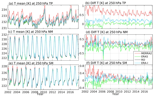
Figure 1 Monthly mean temperature in K at 250 hPa through the three latitude bands of the tropics (TP) (10^∘ S–10^∘ N) (a), northern midlatitudes (NM) (25–45^∘ N) (c), and southern midlatitudes (SM) (25–45^∘ S) (e). Corresponding differences between three reanalyses and the GNSS RO in panels (b), (d) and (f). Models with 103 levels (margin), ERA5 (green), ERA-I (light blue), MERRA2 (red) and GNSS RO (black) are included.

3 Results and analysis

3.1 Time series of temperature

Figure 1 shows the initial time series of zonal mean temperature at 250 hPa from the GNSS RO observations and different reanalyses (ERA5, MERRA2 and ERA-I), as well as the differences between the reanalyses and the GNSS RO data. Three latitude bands are selected to indicate temperature variations in the tropics (TP, 10^∘ S–10^∘ N), midlatitudes in the Northern Hemisphere (NH) (NM, 25–45^∘ N) and midlatitudes in the Southern Hemisphere (SH) (SM, 25–45^∘ S). Seasonal variations are relatively small in the tropics while an evident annual cycle can be seen at midlatitudes of both hemispheres. Generally, reanalyses show good agreement with the GNSS RO in monthly absolute values and seasonal variations, except that MERRA2 shows obviously positive bias compared to other data sets in the TP. As seen from the differences between reanalyses and the GNSS RO, the bias of ERA5 and ERA-I are less than 0.5 K, except at midlatitudes for the period 2002–2006, which shows bias up to 1 K. As the fifth generation of the ECMWF reanalysis, ERA5 shows slightly better agreement than ERA-I in the tropics. Temperature in ERA-I is obviously warmer than the GNSS RO of about 0.1–0.2 K, while ERA5 temperature shows differences of less than 0.1 K compared to the GNSS RO data. Warm biases (0.2 K in NM/SM and 0.7 K in TP) are seen for MERRA2 in all selected regions, which is over 1 K for the period 2002–2006.

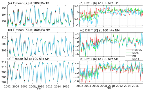
At 100 hPa, as indicated by Fig. 2, more evident seasonal variations in temperature can be seen in the tropics, with similar amplitudes to those at midlatitudes of both hemispheres. Compared to the GNSS RO temperature, ERA-I shows evident cold bias in the tropics during the period 2002–2006. For ERA5, such biases are largely corrected. For the later period 2007–2017, the differences between three reanalyses and the GNSS RO are comparable in magnitude, although the ERA5 shows slightly better agreement with GNSS RO measurements. In midlatitudes of both hemispheres, very similar characteristics can be seen through the three reanalyses, which show slightly better agreement with the GNSS RO than in the tropics. However, relatively large bias can still be seen in the early stage from 2002 to 2006.

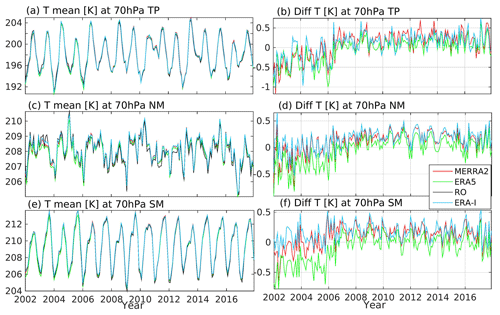
Temperature in the lower stratosphere (70 hPa) shows a clear annual cycle in the tropics (Fig. 3a). However, the annual minimum and maximum values vary year-to-year, which indicate influences from the QBO. Large sub-seasonal fluctuations of temperature can be seen at midlatitudes of the NH, which is obviously different from that in the SH. That is related to strong equatorial and extratropical wave activities in this region. Again, large differences up to 1 K exist between the reanalyses and the GNSS RO observations during the first stage (2002–2006). ERA5 shows obvious cold bias in all selected regions while MERRA2 is anomalously warmer than the GNSS RO in the midlatitudes of both hemispheres. ERA-I, however, has no consistent warm or cold bias and shows the best agreement with the GNSS RO for the period 2002–2006. For the latter stage (2007–2017), ERA5 shows the best agreement with observations (differences within 0.2 K), while the other two reanalyses are slightly (about 0.2 K) warm biased.

Figure 2 As in Fig. 1 but for 100 hPa.

Figure 3 As in Fig. 1 but for 70 hPa.

Note that the bias is particularly large during 2002–2006 for all reanalyses. This should be related to the assimilation of large number of COSMIC data since 2006, which may cause sudden changes in reanalyses (Sturaro, 2003; Sterl, 2004). This helps to explain the weird spiking behavior of 2006 in NM at 250 hPa. At the same time, the GNSS RO data could be also affected by the transition from the single CHAMP satellite to six COSMIC satellites since late 2006. To quantify the sampling errors and bias between two RO missions, we compared COSMIC and CHAMP monthly means for their overlap period of June 2006–September 2008. In addition, the lapse rate tropopause is calculated using the GNSS RO data with the method described in Fueglistaler et al. (2009) and shown in Fig. 4a. Figure 4b shows that COSMIC monthly zonal mean temperatures are consistently colder (0.1–0.2 K) than CHAMP in the stratosphere. The cold is consistent with previous studies (Foelsche et al., 2008; Ho et al., 2009), although the differences between CHAMP and COSMIC are slightly larger than 0.1 K in some areas in the middle stratosphere (50–10 hPa). According to Schrøder et al. (2007) and Leroy et al. (2018), the cold bias between CHAMP and COSMIC is a consequence of a change in the signal-to-noise ratio from 550 in CHAMP to 700 in COSMIC. In addition, the ribbed pattern in the meridional structure of the bias in Fig. 4 is a consequence of a sampling error (Leroy et al., 2018). The bias between COSMIC and CHAMP was computed from the 28-month period of overlap and removed from CHAMP-retrieved temperature for further analysis in this work.

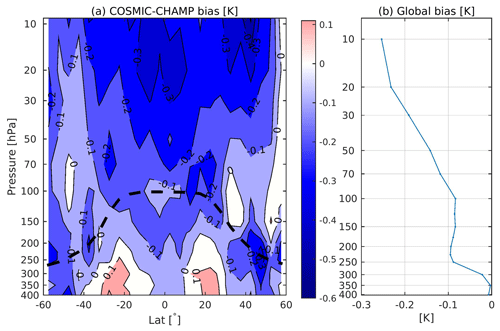
Figure 4 The bias in temperature climatology as retrieved from CHAMP and COSMIC RO data. The two missions obtained data during a 28-month overlap period from June 2006 to September 2008. (a) The difference of monthly zonal mean temperature. (b) The corresponding averaged difference for each layer. The dashed black lines mark the tropopause height calculated with GNSS RO data.

Figure 5 shows differences between three reanalyses and the corrected CHAMP for the period 2002–2006 and COSMIC for the period 2007–2017, respectively. For the first stage, MERRA2 shows a warm bias of 0.1–0.2 K in the upper troposphere, cold bias of 0.1–0.3 K in the lower stratosphere and warm bias of 0.1–0.5 K in the middle stratosphere. ERA5 shows a relatively small cold bias of 0.1–0.2 K for almost the entire UTLS region. ERA-I shows a warm bias of 0.1–0.3 K in the upper troposphere and cold bias of 0.1–0.4 K in the middle stratosphere in both the tropics and the SH. For the second stage, differences between all three reanalysis and the GNSS RO are much smaller. That is because the reanalyses are better constrained by the large number of COSMIC measurements. MERRA2 shows differences with GNSS RO less than 0.1 K, except the cold bias of about 0.2 K at 10 hPa and northern midlatitudes at 200–250 hPa. ERA5 shows perfect agreement with the COSMIC with differences less than 0.1 K in most of the UTLS region, except in northern midlatitudes (100–50 hPa) with a warm bias of 0.1 K. Bias in ERA-I is also quite small with a warm bias of about 0.1 K in the tropics around the tropopause and southern midlatitudes near 10 hPa.

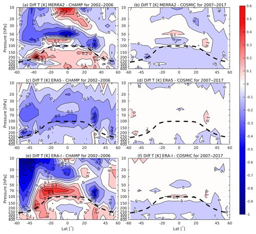
Figure 5 Differences between temperature anomalies between three reanalyses and CHAMP from 400 to 10 hPa for 2002–2006 (a, c, e) and between three reanalyses and COSMIC for 2007–2017 (b, d, f). The dashed black lines mark the tropopause height calculated with GNSS RO data.

In summary, reanalyses show very good agreement with the GNSS RO measurements of sub-seasonal to seasonal variations in temperature in the UTLS region. For the climatological values, a notable change around late 2006 can be found in all reanalyses. Relatively large bias of 0.1–0.5 K can be seen in MERRA2 and ERA-I for the first stage 2002–2006, while very good agreement can be seen between all reanalyses and the GNSS RO measurements for 2007–2017. As the newest reanalysis, ERA5 shows relatively small bias of 0.1–0.3 K during 2002–2006, except in the lowermost stratosphere (70 hPa). In general, ERA5 has the best agreement with GNSS RO. To eliminate the effect of these discontinuities for further studies, reanalysis temperatures were corrected by using a transfer function approach similar to Wargan et al. (2018). The corrected GNSS RO temperature has no significant discontinuities and was used as a common baseline. Details of the bias correction for reanalysis temperatures are provided in the Supplement (Fig. S1).

3.2 Interannual variability of temperature

Figure 6 shows one example of deseasonalized monthly anomalies of temperature in the tropical upper troposphere (10^∘ S–10^∘ N, at 150 hPa). As demonstrated in Fig. 6a, temperature exhibits clear interannual variation, which is related to ENSO and QBO, as indicated by previous studies (Randel and Wu, 2015). While the period of analysis is relatively short, such interannual fluctuations may significantly affect the calculation of linear trends. To estimate the influences of ENSO and QBO, a multiple linear regression method is applied, as introduced in Sect. 3.1. Figure 6d–f indicate contributions of QBO50, QBO30 and ENSO, respectively. ENSO contributes the largest and most significant interannual variations in temperature in the tropical upper troposphere with an amplitude of about 0.5 K, while QBO has only small and insignificant contributions. At lower levels in the free troposphere, the QBO contribution is smaller and the impacts of ENSO are more significant. Reanalyses reveal a very good agreement with each other, as well as the GNSS RO in ENSO-related contributions (Fig. 6f), but show larger spread for QBO contributions. For the shorter period, the interannual variability should have more influence on the trend calculations. Through such a multiple linear regression, the influences of ENSO and QBO and the linear trend can be separated. As seen in Figure 6c, GNSS RO indicates an increase of 0.4 K in temperature for the whole period 2002–2017. ERA-I trend is smallest (0.1 K per decade). According to Simmons et al. (2014), local degradation occurs near the subtropical tropopause, whereas substantial amounts of warm-biased aircraft data have been assimilated since 1999. After 2006, when a large number of COSMIC data were assimilated, this warm bias disappeared. This anomalous warm temperature for the short period 1999–2005 leads to less warming in this region in the estimated ERA-I time series. Such bias has been corrected in ERA5 temperature data. ERA5 clearly shows better agreement with GNSS RO.

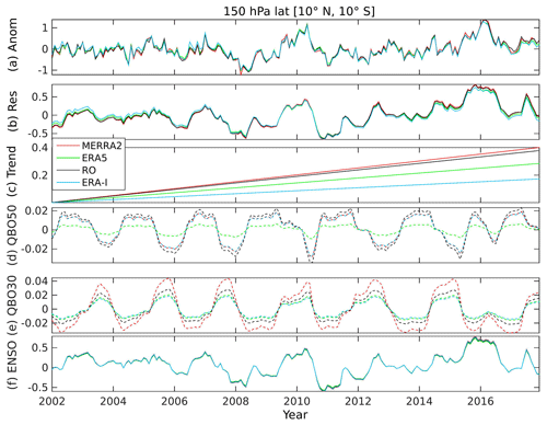
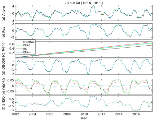
Figure 6 Temperature anomaly at 150 hPa in the tropics (10^∘ S–10^∘ N) from ERA5 (green), ERA-I (light blue), MERRA2 (red) and GNSS RO (black) (a). (b) The corresponding residual. (c) The linear terms. (d) The QBO50 terms. (e) The QBO30 terms and (f) the ENSO terms. The solid lines in (c–f) mark the significant terms and the dashed lines in (c–f) mark the insignificant terms.

Figure 7 As in Fig. 6 but for 70 hPa.

In the lower stratosphere, as illustrated in Fig. 7, interannual variations in temperature are dominated by QBO, with amplitudes of over 1 K for QBO50. The ENSO effects are insignificant, with an amplitude of about 0.5 K. GNSS RO indicates an increase of 0.55 K, as seen in Fig. 7c. MERRA2 and ERA-I/ERA5 show a similar increase of 0.65–0.7 K, which is stronger than GNSS RO. The relative contributions of ENSO and QBO to interannual variations in zonal mean temperatures in the UTLS are shown in Figs. 8–10.

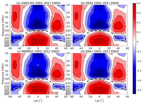
Figure 8 ENSO-related temperature anomalies of GNSS RO (a), ERA5 (b), MERRA2 (c) and ERA-I (d). The dashed black lines mark the tropopause height calculated with GNSS RO data.

Consistent with previous studies (Randel and Wu, 2015), positive ENSO is associated with warm temperature anomalies of 0.1–0.4 K in the tropical upper troposphere and cold temperature anomalies of 0.1–0.5 K above the tropopause in the tropics (Fig. 8). In contrast with the tropics, anomalous cold temperatures can be seen in the subtropics below 100 hPa, while warm temperature anomalies exist above 100 hPa. All three reanalyses show consistent patterns, as seen in GNSS RO associated with positive ENSO.

Figure 9 As in Fig. 8 but for QBO50.

Figure 10 As in Fig. 8 but for QBO30.

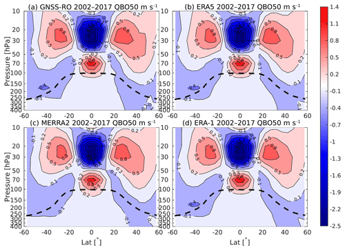
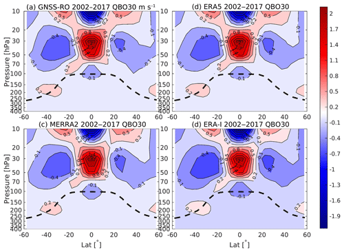
As a stratospheric phenomenon, westerly QBO affects the temperature mainly in the upper atmosphere above 100 hPa. The spatial structure of temperature anomalies associated with wind terms, in meters per second, of QBO50 and QBO30 are shown in Figs. 9–10. QBO50 is associated with warming in the lowermost stratosphere (100–50 hPa) and cooling in middle stratosphere (50–15 hPa) in the tropics. Subtropics and midlatitudes, however, show out-of-phase variations with significant warming signals. QBO30 contributes to similar temperature variations, except that the signals are spatially orthogonal with the patterns associated with QBO50 (Fig. 10). Reanalyses show very good agreement with GNSS RO in both spatial pattern and magnitude for QBO-related temperature variations, as illustrated in Figs. 9–10.

3.3 Temperature trends

Figure 11 summarizes the spatial distribution of temperature trends based on corrected GNSS RO and reanalyses for the time period 2002–2017. From the GNSS RO measurements, positive trends of 0.2–0.3 K per decade are significant in most areas of the troposphere, with stronger warming up to 0.4–0.5 K per decade at the midlatitudes of both hemispheres. At the same time, negative trends of 0.1–0.3 K per decade are evident in the stratosphere (50–10 hPa). In the lowermost stratosphere (100–50 hPa), positive temperature trends exist in the tropics, although the trends at 50 hPa are less significant. This is consistent with previous studies (Wang et al., 2013, 2015; Polvani et al., 2017), which indicated a warming in this region since 2001. However, the trends shown here (0.3 K per decade maximum) are much smaller than those in their results (e.g., up to 1.6 K per decade in Wang et al., 2013). As seen from the time series of temperature at 70 hPa (Fig. 7), the temperature increases from 2002 until 2011 and then declines (or stop to increase) after that.

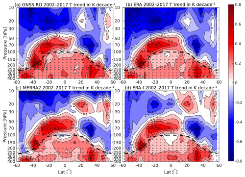
Figure 11 Temperature trend in K per decade based on GNSS RO (a), ERA5 (b), MERRA2 (c) and ERA-I (d) data for the period 2002–2017. The “+” marks the significant area at 95 % level. The dashed black lines mark the tropopause height calculated with GNSS RO data.

Reanalysis data show good agreement with the GNSS RO for the general pattern of temperature trends. However, slightly smaller trends are found in MERRA2 in the tropical free troposphere (400–200 hPa), which could be related to the observed warm bias during 2002–2006 in MERRA2, as illustrated in Fig. 5. ERA-I shows neutral trends around 150–100 hPa in the tropics (15^∘ S–15^∘ N), which are positive in other data sets and should be also related to the warm-biased aircraft data, as mentioned in Sect. 3.2. Very good agreement can be seen between ERA5 and the GNSS RO data in the troposphere with a very similar spatial pattern and comparable magnitude of warm in the troposphere.

In the stratosphere, the negative trends in ERA-I are too weak and less significant in the SH. At the same time, positive trends in the NH are stronger in both MERRA2 and ERA-I than those in GNSS RO. ERA5 shows the best agreement with GNSS RO measurements with a consistent pattern and comparable magnitude. At 10 hPa in the tropics, all the data sets show negative trends except ERA-I. According to Simmons et al. (2014), the large differences between MERRA2 and ERA-I at 10 hPa are associated with differing treatments of the change from SSU to AMSU-A and the availability of increasing amounts of largely unadjusted radiosonde data. While cell pressure correction to SSU has been done in ERA5, it shows similar cooling trends to observations at 10 hPa. Notable differences between GNSS RO and reanalyses can also be seen in the tropics (5^∘ S–20^∘ N) around the lapse rate tropopause. Neutral trends are found by GNSS RO and ERA-I in this region, while ERA5 shows insignificant positive trends (0.2 K per decade) and MERRA2 shows insignificant negative trends (−0.1 K per decade). As a transition zone between the troposphere and the stratosphere, the opposite sign could appear in neighboring layers below or above the tropopause, which causes large uncertainties in estimated trends around the tropopause.

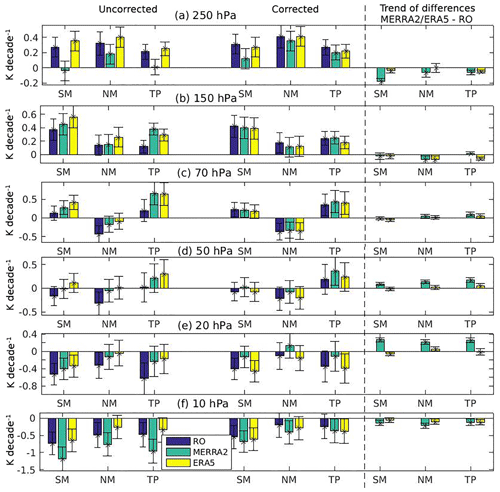
Figure 12 Estimated temperature trends in K per decade in different regions (SM: 25–45^∘ S; NM: 25–45^∘ N; TP: 10^∘ S–10^∘ N) from 2002 to 2017. (a–f) Trends in corrected and uncorrected data sets at 250, 150, 70, 50, 20 and 10 hPa. Trends based on the differences of time series between MEMRRA2/ERA5 and GNSS RO are also shown to the right of the figure. Error bars represent 95 % confidence intervals.

Figure 12 further illustrates the temperature trends based on uncorrected and corrected GNSS RO and reanalysis data sets in three regions (SM: 25–45^∘ S; NM: 25–45^∘ N; TP: 10^∘ S–10^∘ N) at selected pressure levels (250, 150, 70, 50, 20, 10 hPa). The temperature increase in the upper troposphere is stronger and the cooling in the stratosphere gets weaker after the correction of the GNSS RO data. The differences of temperature trends between the reanalysis and GNSS RO measurements become much smaller after corrections. For example, MERRA2 shows significant warming at 250 hPa in the SM after the correction, which is more consistent with the GNSS RO data. The unrealistically strong cooling in MERRA2 at 10 hPa is significantly reduced by the correction. Overall, the reanalysis data represent the temperature trends well from the upper troposphere to the mid-stratosphere after the correction, although obvious differences can be seen between the reanalysis and the GNSS RO measurements. As the newest reanalysis, ERA5 shows the best agreement with the GNSS RO measurements among most of areas, as demonstrated in this study.

Note that the temperature trends discussed above are based on a relatively short data record of 16 years. The statistical significance of the obtained trends must be carefully discerned since the trend assessment from such a short period can be strongly influenced by start and end years (Bandoro et al., 2018; Santer et al., 2017). Besides the two-sided Student's t test, mentioned in Sect. 2.5, a signal-to-noise study is also included. The background noise of 16-year temperature trends are estimated by three fully coupled CESM simulations, which were integrated over 145 years (1955 to 2099) with anthropogenic emissions (GHGs and ODSs) fixed to values at 1960. We fit linear trends to overlapping 192-month segments of the 1740 months in each of CESM runs and then the noise can be calculated by the standard deviation of the 16-year trends. More details of the CESM simulations and the methods can be seen in the Supplement. The signal-to-noise ratios of 16-year GNSS RO temperature trends are shown in Fig. S2. As seen in Fig. S2, the areas with significant trends are smaller than those shown in Fig. 11, especially in the tropics. This indicates that large uncertainties exist in the trends, as shown in Fig. 11 in the tropics. However, there are still significant signals in the midlatitudes of the upper troposphere, around the tropopause and in the SH in the middle stratosphere. All of the significant regions in Fig. S2 are actually the most important areas with the strongest and most significant trends in Fig. 11. This suggests that the significant trends shown in Fig. 11 are robust, except in the tropics where the standard deviation of the trends are the strongest.

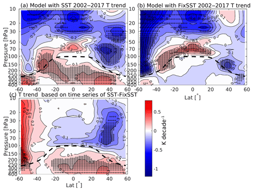
Figure 13 Temperature trends in K per decade based on model simulations with time-varying SST (a), fixed SST (b) and their differences (c) for the period 2002–2017. The “+” marks trends found to be more than 95 % statistically significant. The dashed black lines mark the tropopause height calculated with GNSS RO data.

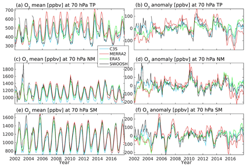
Figure 14 Monthly mean ozone in ppbv at 70 hPa through three latitude bands of TP (10^∘ S–10^∘ N) (a), NM (25–45^∘ N) (c), and NM (25–45^∘ S) (e). Corresponding anomalies in panels (b), (d) and (e). Model with 103 levels (margin), ERA5 (green), C3S (light blue), MERRA2 (red) and SWOOSH (black) are included. The dashed black lines mark the tropopause height calculated with GNSS RO data.

To explain the underlying mechanisms, such as dynamical processes associated with SST of the illustrated temperature trends, two WACCM simulations, as described in Sect. 2.4, were employed. Figure 13 shows the temperature trends from the transient run and the fixed SST run, as well as their differences. The transient run with varying SST (Fig. 13a) shows comparable positive trends (0.2–0.3 K per decade) in the troposphere and negative trends (0.1–0.5 K per decade) in the stratosphere (see Fig. 11 for comparison). While the SSTs are fixed to climatological values, which means only radiative effects from GHGs and ODSs are included, the positive trends in the troposphere disappear or become much weaker (Fig. 13b). This reveals that the influences of SSTs on circulation are the main reason for the warming temperature trends in the troposphere, which can be confirmed by the differences between these two runs (Fig. 13c). The negative temperature trends in the stratosphere (tropics and SH) persist in the fixed SST run, which illustrates that other factors like radiative effects from GHGs and ozone contribute to such cooling. For the temperature trends above the tropical tropopause (100–50 hPa), the weak warming is related to combined effects of SSTs (that contribute to a cooling) and other effects (that lead to a warming).

3.4 Coupling with ozone

Figure 14 shows the initial ozone time series from SWOOSH, C3S, MERRA2 and ERA5, as well as their differences, using the SWOOSH data as a reference in three regions at 70 hPa. The ERA-I is not included here for ozone analysis because it does not assimilate as many ozone measurements as ERA5 and MERRA2. Although the phase and amplitude agree well in general, the absolute ozone values have large differences between different data sets. Obvious missing data and extreme values exist in both SWOOSH and C3S data sets during 2002–2004, while a discontinuity in the MERRA2 and ERA5 time series occurs in mid-2004 when the Aura MLS mission started. As illustrated in Fig. 14, extremely large values are observed by SWOOSH and C3S around 2003. The reason is the limited number of observations in this period, which could cause large sampling errors and uncertainties in ozone data. At the same time, since the reanalysis is less constrained during this period, large bias can be seen in both MERRA2 and ERA5 compared to observations (Fig. 14b, d and f). After 2006, SWOOSH only uses MLS ozone data (Davis et al., 2016), and MERRA2 has also used MLS instead of SBUV ozone data since October 2004 (Gelaro et al., 2017). Therefore, the MERRA2 ozone data have good agreement with SWOOSH data. Another discontinuity in the MERRA2 and ERA5 time series occurs around 2015. According to McCarty et al. (2016), MERRA2 started to use the version 4.2 MLS ozone data instead of version 2.2 in June 2015, which causes data discontinuities at 250–70 hPa. As seen in Fig. 14b, d and f, ozone in MERRA2 is 50–150 ppbv lower than that in SWOOSH and C3S. ERA5 combined more satellite data (SBUV and MLS) than MERRA2, which leads to larger variability of ozone in ERA5 since the different data sets and different ways for merging the data have large influences on the ozone data. The missing data and extreme values in SWOOSH and C3S, as well as the data discontinuities in MERRA2 and ERA5 around 2004 and 2015, can also be seen at other pressure levels (see Figs. S3–S4 for details).

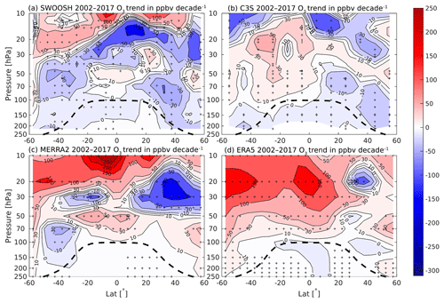
Figure 15 Ozone trend in ppbv per decade based on SWOOSH (a), ERA5 (b), MERRA2 (c) and C3S (d) data for period 2002–2017. The “+” marks trends found to be more than 95 % statistically significant. The dashed black lines mark the tropopause height calculated with GNSS RO data.

To examine the connection between the vertical temperature changes and ozone distribution, ozone trends are analyzed in the stratosphere from 250 to 10 hPa. In consideration of the discontinuities in MERRA2 and ERA5 around late 2004 due to the MLS ozone data, a step function proxy is added for January 2002–September 2004 in the trend calculation. An extra step function proxy is added in the MERRA2 MLR to remove the discontinuities associated with the transition from MLS v2.2 to v4.2 for 250–70 hPa for the period June 2015–December 2017. The trends are calculated for the period 2002–2017 using the same MLR method as for temperature but with step function proxies in the reanalyses (Fig. 15). Large discrepancies exist in the ozone trends between the two merged satellite data sets (Fig. 15a and b), which makes it hard to decide the actual trends of ozone for the period 2002–2017. This may be related to the large number of missing values in satellite observations in the early stages of 2002–2004. While the trends are calculated from 2005 to 2017, the two data sets are more consistent with each other (not shown). Consistent negative trends in the NH lowermost stratosphere (150–50 hPa) and in the middle stratosphere (30–10 hPa) can be seen in both the SWOOSH and the C3S data sets, while the positive ozone trends in the tropical lower stratosphere (100–50 hPa) are also in good agreement. Asymmetry trends in two hemispheres, with a significant decrease in ozone in NH midlatitudes at 100–10 hPa and an increase in ozone in SH midlatitudes, are found at 30–10 hPa. This is consistent with a recent study using the MLS ozone data (Chipperfield et al., 2018). Ozone trends in the reanalyses are different from the merged satellite data sets as well as between each other. The only agreement can be seen in the positive trends of ozone in the lowermost stratosphere (150–50 hPa) in the tropics.

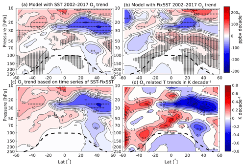
Figure 16 Ozone trend in ppbv per decade based on model simulations with time-varying SST (a), fixed SST (b) and their differences, SST–fixed SST (c), for the period 2002–2017. (d) Model ozone-related GNSS RO temperature trends in K per decade. The “+” marks trends found to be more than 95 % statistically significant. The dashed black lines mark the tropopause height calculated with GNSS RO data.

Figure 16 shows the ozone trends from two model simulations as well as their differences. The ozone trends, based on the model simulation with varying SSTs, show similar trends to SWOOSH and C3S data for their consistent trends in the NH lowermost stratosphere (150–50 hPa), the NH mid-stratosphere (30–10 hPa) and the tropical lower stratosphere (100–50 hPa). While the SSTs are fixed to climatological values, ozone increases from the tropics to SH midlatitudes in the middle stratosphere (30–10 hPa), and negative trends in the NH midlatitudes from 30 to 10 hPa become much weaker (Fig. 16b). The negative ozone trends in the NH lower stratosphere (150–50 hPa) seen in Fig. 16a are the opposite of those in Fig. 16b. The differences between these two runs, which indicate contributions from SSTs, show a similar spatial pattern to the transient run and observations. This confirms that dynamic processes dominate ozone trends in the lower (150–50 hPa) and middle stratosphere (30–10 hPa) in the NH, which is consistent with the previous study (Chipperfield et al., 2018). For the tropical lower stratosphere (20^∘ S–20^∘ N, 100–50 hPa), ozone trends are determined by a combination of ODSs and SSTs (Fig. 16b–c).

Considering the coupling between changes in ozone and temperature, the correlation coefficients are calculated between ozone and temperature anomalies for the period 2002–2017. Consistent with previous studies (Abalos et al., 2012; Maycock, 2016; Gilford et al., 2016), observed ozone (GNSS RO) and temperature (SWOOSH) anomalies are highly correlated (>0.6) in the range from 100 to 20 hPa (Fig. S5a). The correlation coefficients are highest in the tropical region (∼ 0.9). MERRA2 shows a similar correlation between ozone and temperature, while the correlation in ERA5 is slightly weaker. Furthermore, we estimate a factor b_f(p) between temperature and ozone anomalies at each grid point p by linear regression:

$$\begin{array}{}\text{(2)}& {\displaystyle }y(p,t)=b_{\mathrm{f}}\left(p\right)\cdot x(p,t),\end{array}$$

where y(p,t) is the monthly temperature anomalies and x(p,t) is the monthly ozone anomalies at each grid point p. Then the potential contribution of ozone changes to temperature trends T(p) is estimated by the ozone trend O₃(p) and b_f(p) with Eq. (3) (Figs. 16d and S6d).

$$\begin{array}{}\text{(3)}& {\displaystyle }T\left(p\right)={\mathrm{O}}_{\mathrm{3}}\left(p\right)\cdot b_{\mathrm{f}}\left(p\right)\end{array}$$

While ozone and temperature are positively correlated, a decrease in ozone contributes to a cooling in the NH and in the tropical upper troposphere and mid-stratosphere. Increases in ozone lead to a warming effect in the SH and the lower stratosphere in the tropics.

Recalling the question of the temperature trend attribution, the positive trends in the upper troposphere can be explained well by increases in SSTs (Fig. 13). The stratospheric cooling, however, can not be fully explained. Satellite measurements show a stronger cooling in the SH than in the NH. Model simulation and ozone–temperature correlations indicate that both SST and ozone changes contribute to a cooling in the NH but a warming in the SH. The exact reason for the strong cooling in the lower to mid-stratosphere in the SH awaits further study. The tropical warming in the lower stratosphere is related to both SST and ozone changes. As seen in Fig. S6, SSTs significantly increased during 2002–2017 almost globally, except in the North Atlantic and the Southern Ocean. Such an increase in SSTs would warm up the troposphere and lead to strengthening in the upward motion of the atmosphere, which leads to a cooling in the tropical lower stratosphere. At the same time, ozone is increased and contributes to a warming in that region (Figs. 16 and S5) . As indicated by Wang et al. (2015), the increase in temperature in the tropical lower stratosphere is dominated by an anomalous SST decline from 2001 to 2011. While a significant increase in SST occurs after 2011, the temperature in the tropical lower stratosphere decreases and leads to a net cooling for the period 2002–2017. Ozone increases from 2002 to 2017 and contributes to a warming effect to the tropical lower stratosphere. However, the potential contribution of ozone to temperature in the tropical lower stratosphere is quite weak, which can not fully explain the observed warming in that region.

4 Conclusions and discussion

The recent variability and trends of temperature in the UTLS have been studied for the period 2002–2017 using high-quality, high vertical resolution GNSS RO data. The newest ERA5 reanalysis product, as well as the MERRA2 and the ERA-I reanalyses, is evaluated for seasonal-to-interannual variations and linear trends of temperature in the UTLS.

In general, all three reanalyses show good agreement with the GNSS RO measurements for the annual cycle of temperature with a consistent phase and comparable amplitude. However, relatively large biases can be seen between reanalysis data set and GNSS RO for the period 2002–2006, which reveals an evident discontinuity of temperature time series in reanalyses. This is caused by the lack of observations and less constrained reanalysis data in the first stage and the large amounts of data from the COSMIC satellite mission since 2007. Such discontinuity in reanalysis data should be carefully considered while using the reanalysis data for analyzing trends. ERA5 shows obvious improvements in temperature data compared to ERA-I and also a slightly better agreement with GNSS RO measurements than MERRA2.

Temperature in the UTLS presents significant interannual variations, which are known to be related to ENSO and QBO. Based on a multiple linear regression method, the relative contributions of ENSO and a pair of orthogonal time series of QBO (QBO50 and QBO30) are estimated from the GNSS RO measurements and reanalysis data sets. Signals of ENSO and QBO show very good agreement between all three reanalyses and the GNSS RO data, which indicates that the reanalyses are able to capture interannual variations in temperature in the UTLS.

A total of 16 years of temperature data were analyzed by a MLR method to determine trends in the UTLS. A significant warming of 0.2–0.3 K per decade can be seen in most areas of the troposphere with a stronger increase of 0.4–0.5 K per decade at the midlatitudes of both hemispheres. In contrast with the troposphere, the stratospheric temperature decreases at a rate of 0.1–0.3 K per decade. Positive temperature trends are significant in the tropical lower stratosphere (100–50 hPa) with a much weaker magnitude (0.1–0.5 K per decade) than that in an earlier period (2001–2011), as shown by a previous study (Wang et al., 2015). Again, ERA5 shows improved quality compared to ERA-I and has the best agreement with the GNSS RO data in the three reanalyses. MERRA2 shows less significant warming trends in the tropical troposphere and an overly strong cooling in its initial data but more consistent trends after the discontinuity corrections.

Similar to temperature data, reanalysis ozone is affected by the change of assimilated observations and methods. Negative trends of ozone are dominant in the NH at 150–50 hPa. In the tropical lower stratosphere, increases in ozone are evident. Asymmetric trends of ozone can be found for the two hemispheres in the middle stratosphere, with significant ozone decreases in NH midlatitudes and increases in ozone in SH midlatitudes. Around the tropopause, trends are small and large differences between data sets are found. Further study and longer time series are needed for trend analyses in these regions. Overall, large biases exist in reanalysis and it is still challenging to do trend analysis based on reanalysis ozone data.

According to model simulations, the temperature increase in the troposphere and the ozone decrease in the NH stratosphere could be mainly connected to the increase in SST and subsequent changes of atmospheric circulations. Ozone increases around 20 hPa in the SH, decreases around 30 hPa and increases from 20 to 10 hPa in the tropics are also closely related to SST changes. This supports the results of Chipperfield et al. (2018), which concluded that dynamical changes play an important role in the ozone variability in the stratosphere. Ozone increases in the tropical lower stratosphere may be related to reduced emissions of ODSs since the adoption of Montreal Protocol (Polvani et al., 2017) and are partly offset by SST changes.

In the stratosphere, ozone and temperature variations are highly correlated with each other. Due to the radiative effects of ozone, a decrease in ozone in the NH contributes partly to the temperature decrease in this region. The increased ozone may contribute to the temperature increase in the tropical lower stratosphere. However, this contribution from ozone is relatively weak and can not fully explain the warming in those regions. In addition, it is partly offset by the cooling effect of increases in SSTs. The long-term trend of temperature in the lower stratosphere is strongly modified by interannual and decadal fluctuations related to natural processes like SST variations.

Recent temperature and ozone trends have been calculated by a MLR method based on observational data sets. However, trend assessments over short period of 1–2 decades are largely uncertain, since the calculated trends are sensitive to start or end date (Santer et al., 2017). As RO data are acquired over longer periods with a large number of observations (more than 10 000 per day) by COSMIC2, the climate signal will emerge robustly and be more reliable for the temperature trends and variability studies in the UTLS.